MacroPCA: An all-in-one PCA method allowing for missing values as well as cellwise and rowwise outliers
Abstract
Multivariate data are typically represented by a rectangular matrix (table) in which the rows are the objects (cases) and the columns are the variables (measurements). When there are many variables one often reduces the dimension by principal component analysis (PCA), which in its basic form is not robust to outliers. Much research has focused on handling rowwise outliers, i.e. rows that deviate from the majority of the rows in the data (for instance, they might belong to a different population). In recent years also cellwise outliers are receiving attention. These are suspicious cells (entries) that can occur anywhere in the table. Even a relatively small proportion of outlying cells can contaminate over half the rows, which causes rowwise robust methods to break down. In this paper a new PCA method is constructed which combines the strengths of two existing robust methods in order to be robust against both cellwise and rowwise outliers. At the same time, the algorithm can cope with missing values. As of yet it is the only PCA method that can deal with all three problems simultaneously. Its name MacroPCA stands for PCA allowing for Missingness And Cellwise & Rowwise Outliers. Several simulations and real data sets illustrate its robustness. New residual maps are introduced, which help to determine which variables are responsible for the outlying behavior. The method is well-suited for online process control. Supplementary material is available online.
Keywords: Detecting deviating cells, Outlier map, Principal component analysis, Residual map, Robust estimation.
1 Introduction
Real data often contain outliers, which can create serious problems when analyzing it. Many methods have been developed to deal with outliers, often by constructing a fit that is robust to them and then detecting the outliers by their large deviation (distance, residual) from that fit. For a brief overview of this approach see Rousseeuw and Hubert (2018). Unfortunately, most robust methods cannot handle data with missing values, some rare exceptions being Cheng and Victoria-Feser (2002) and Danilov et al. (2012). Moreover, they are typically restricted to casewise outliers, which are cases that deviate from the majority. We call these rowwise outliers because multivariate data are typically represented by a rectangular matrix in which the rows are the cases and the columns are the variables (measurements). In general, robust methods require that fewer than half of the rows are outlying, see e.g. Lopuhaä and Rousseeuw (1991). However, recently a different type of outliers, called cellwise outliers, have received much attention (Alqallaf et al., 2009; Van Aelst et al., 2012; Agostinelli et al., 2015). These are suspicious cells (entries) that can occur anywhere in the data matrix. Figure 1 illustrates the difference between these types of outliers. The regular cells are shown in gray, whereas black means outlying. Rows 3 and 7 are rowwise outliers, and the other rows contain a fairly small percentage of cellwise outliers. As in this example, a small proportion of outlying cells can contaminate over half the rows, which causes most methods to break down. This effect is at its worst when the dimension (the number of columns) is high.
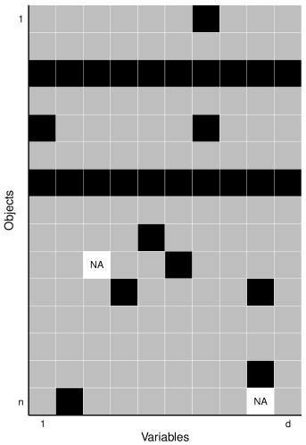
In high-dimensional situations, which are becoming increasingly common, one often applies principal component analysis (PCA) to reduce the dimension. However, the classical PCA (CPCA) method is not robust to either rowwise or cellwise outliers. Robust PCA methods that can deal with rowwise outliers include Croux and Ruiz-Gazen (2005), Hubert et al. (2002), Locantore et al. (1999), Maronna (2005) and the ROBPCA method (Hubert et al., 2005). The latter method combines projection pursuit ideas with robust covariance estimation.
In order to deal with missing values, Nelson et al. (1996) and Kiers (1997) developed the iterative classical PCA algorithm (ICPCA), see Walczak and Massart (2001) for a tutorial. The ICPCA follows the spirit of the EM algorithm. It starts by replacing the missing values by initial estimates such as the columnwise means. Then it iteratively fits a CPCA, yielding scores that are transformed back to the original space resulting in new estimates for the missing values, until convergence.
Serneels and Verdonck (2008) proposed a rowwise robust PCA method that can also cope with missing values. We will call this method MROBPCA (ROBPCA for missing values) as its key idea is to combine the ICPCA and ROBPCA methods. MROBPCA starts by imputing the NA’s by robust initial estimates. The main difference with the ICPCA algorithm is that in each iteration the PCA model is fit by ROBPCA, which yields different imputations and flags rowwise outliers.
As of yet there are no PCA methods that can deal with cellwise outliers in combination with rowwise outliers and NA’s. This paper aims to fill that gap by constructing a new method called MacroPCA, where ‘Macro’ stands for Missingness And Cellwise and Rowwise Outliers. It starts by applying a multivariate method called DetectDeviatingCells (Rousseeuw and Van den Bossche, 2018) for detecting cellwise outliers, which provides initial imputations for the outlying cells and the NA’s as well as an initial measure of rowwise outlyingness. In the next steps MacroPCA combines ICPCA and ROBPCA to protect against rowwise outliers and to create improved imputations of the outlying cells and missing values. MacroPCA also provides graphical displays to visualize the different types of outliers. R code for MacroPCA is publicly available (Section 8).
2 The MacroPCA algorithm
2.1 Model
The data matrix is denoted as in which the subscripts are the number of rows (cases) and the number of columns (variables) . In the absence of outliers and missing values the goal is to represent the data in a lower dimensional space, i.e.
| (1) |
with the column vector with all components equal to 1, the -variate column vector of location, the score matrix, the loadings matrix whose columns span the PCA subspace, and the error matrix. The reduced dimension can vary from 1 to but we assume that is low. The , and are unknown, and estimates of them will be denoted by , and .
Several realities complicate this simple model. First, the data matrix may not be fully observed, i.e., some cells may be missing. Here we assume that they are missing at random (MAR), meaning that the missingness of a cell is unrelated to the value the cell would have had, but may be related to the values of other cells in the same row; see, e.g., Schafer and Graham (2002). This is the typical assumption underlying EM-based methods such as ICPCA and MROBPCA that are incorporated in our proposal.
Secondly, the data may contain rowwise outliers, e.g. cases from a different population. The existing rowwise robust methods require that fewer than half of the rows are outlying, so we make the same assumption here.
Thirdly, cellwise outliers may occur as described in the introduction. The outlying cells may be imprecise, incorrect or just unusual. Outlying cells do not necessarily stand out in their column because the correlations between the columns matter as well, so these cells may not be detectable by simple univariate outlier detection methods. There can be many cellwise outliers, and in fact each row may contain one or more outlying cells.
2.2 Dealing with missing values and cellwise and rowwise outliers
We propose the MacroPCA algorithm for analyzing data that may contain one or more of the following issues: missing values, cellwise outliers, and rowwise outliers. Throughout the algorithm we will use the following two notations:
-
•
the NA-imputed matrix only imputes the missing values of ;
-
•
the cell-imputed matrix has imputed values for the outlying cells that do not belong to outlying rows, and for all missing values.
Both of these matrices still have rows. Neither is intended to simply replace the true data matrix . Note that does not try to impute outlying cells inside outlying rows, which would mask these rows in subsequent computations.
Since we do not know in advance which cells and rows are outlying, the set of flagged cellwise and rowwise outliers (and hence and ) will be updated in the course of the algorithm.
The first part of MacroPCA is the DetectDeviatingCells (DDC) algorithm. The description of this method can be found in Rousseeuw and Van den Bossche (2018) and in Section 1 of the Supplementary Material. The main purpose of the DDC method is to detect cellwise outliers. DDC outputs their positions as well as imputations for these outlying cells and any missing values. It also yields an initial outlyingness measure on the rows, which is however not guaranteed to flag all outlying rows. The set of flagged rows will be improved in later steps.
The second part of MacroPCA constructs principal components along the lines of the ICPCA algorithm but employing a version of ROBPCA (Hubert et al., 2005) to fit subspaces. It consists of the following steps, with all notations listed in Section 2 of the Supplementary Material.
-
1.
Projection pursuit. The goal of this step is to provide an initial indication of which rows are the least outlying. For this ROBPCA starts by identifying the least outlying rows by a projection pursuit procedure. We write . This means that we can withstand up to a fraction of outlying rows. To be on the safe side the default is .
However, due to cellwise outliers there may be far fewer than uncontaminated rows, so we cannot apply this step to the original data . We also cannot use the entire imputed matrix obtained from DDC in which all outlying cells are imputed, even those in potentially outlying rows, as this could mask outlying rows. Instead we use the cell-imputed matrix defined as follows:
-
(a)
In all rows flagged as outlying we keep the original data values. Only the missing values in these rows are replaced by the values imputed by DDC. More precisely, for all in we set .
-
(b)
In the unflagged rows with the fewest cells flagged by DDC we impute those cells, i.e. .
As in ROBPCA the outlyingness of a point is then computed as
(2) where and are the univariate MCD location and scale estimators (Rousseeuw and Leroy, 1987) of . The set contains 250 directions through two data points (or all of them if there are fewer than 250). Finally, the indices of the rows with the lowest outlyingness and not belonging to are stored in the set .
-
(a)
-
2.
Subspace dimension. Here we choose the number of principal components. For this we build a new cell-imputed matrix which imputes the outlying cells in the rows of and imputes the NA’s in all rows. This means that for , and if . Then we apply classical PCA to the with . Their mean is an estimate of the center, whereas the spectral decomposition of their covariance matrix yields a loading matrix and a diagonal matrix with the eigenvalues sorted from largest to smallest. These eigenvalues can be used to construct a screeplot from which an appropriate dimension of the subspace can be derived. Alternatively, one can retain a certain cumulative proportion of explained variance, such as 80%. The maximal number of principal components that MacroPCA will consider is the tuning constant which is set to 10 by default.
-
3.
Iterative subspace estimation. This step aims to estimate the -dimensional subspace fitting the data. As in ICPCA this requires iteration, for :
-
(a)
The scores matrix in (1) based on the cell-imputed cases is computed as . The predicted data values are set to . We then update the imputed matrices to and by replacing the appropriate cells by the corresponding cells of . That is, for we update all the imputations of missing cells, whereas for we update the imputations of the outlying cells in rows of as well as the NA’s in all rows.
-
(b)
The PCA model is re-estimated by applying classical PCA to the with . This yields a new estimate as well as an updated loading matrix .
The iterations are repeated until or until convergence is reached, i.e. when the maximal angle between a vector in the new subspace and the vector most parallel to it in the previous subspace is below some tolerance (by default 0.005). Following Krzanowski (1979) this angle is computed as where is the smallest eigenvalue of .
After all iterations we have the cell-imputed matrix as well as the estimated center and the loading matrix .
-
(a)
-
4.
Reweighting. In robust statistics one often follows an initial estimate by a reweighting step in order to improve the statistical efficiency at a low computational cost, see e.g. (Rousseeuw and Leroy, 1987; Engelen et al., 2005). Here we use the orthogonal distance of each to the current PCA subspace:
The orthogonal distances to the power 2/3 are roughly Gaussian except for the outliers (Hubert et al., 2005), so we compute the cutoff value
(3) All cases for which are considered non-outlying with respect to the PCA subspace, and their indices are stored in a set . As before, any is removed from . The cases not in are flagged as rowwise outliers. The final cell-imputed matrix is given by if and and otherwise. Applying classical PCA to the rows in yields a new center and a new loading matrix .
-
5.
DetMCD. Now we want to estimate a robust basis of the estimated subspace. The columns of from step 4 need not be robust, because some of the rows in might be outlying inside the subspace. These so-called good leverage points do not harm the estimation of the PCA subspace but they can still affect the estimated eigenvectors and eigenvalues, as illustrated by a toy example in Section A.1 of the Appendix. In this step we first project the points of onto the subspace, yielding
Next, the center and scatter matrix of the scores are estimated by the DetMCD method of Hubert et al. (2012). This is a fast, robust and deterministic algorithm for multivariate location and scatter, yielding and . Its computation is feasible because the dimension of the subspace is quite low. The spectral decomposition of yields a loading matrix and eigenvalues for . We set the final center to and the final loadings to .
-
6.
Scores, predicted values and residuals. We now provide the final output. We compute the scores of as and the predictions of as . (The formulas for and are analogous.) This yields the difference matrix which we then robustly scale by column, yielding the final standardized residual matrix . The orthogonal distance of to the PCA subspace is given by
(4)
See Section 8 for the R code carrying out MacroPCA.
MacroPCA can be carried out in time (seeSection A.2 of the Appendix) which is not much more than the complexity of classical PCA. Figure 2 shows times as a function of and indicating that MacroPCA is quite fast. The fraction of NA’s in the data had no substantial effect on the computation time, as seen in Figure 15 in Section A.2.
 |
 |
Note that PCA loadings are highly influenced by the variables with the largest variability. For this the MacroPCA code provides the option to divide each variable by a robust scale. This does not increase the computational complexity.
3 Outlier detection
MacroPCA provides several tools for outlier detection. We illustrate them on a dataset collected by Alfons (2016) from the website of the Top Gear car magazine. It contains data on 297 cars, with 11 continuous variables. Five of these variables (price, displacement, BHP, torque, top speed) are highly skewed, and were logarithmically transformed. The dataset contains 95 missing cells, which is only 2.9% of the cells. We retained two principal components ().
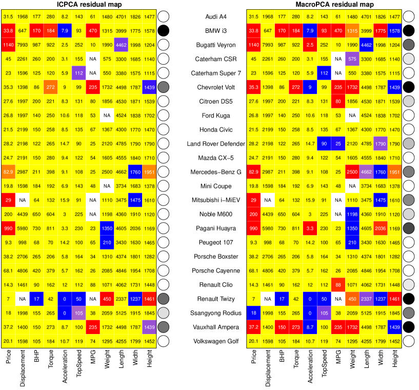
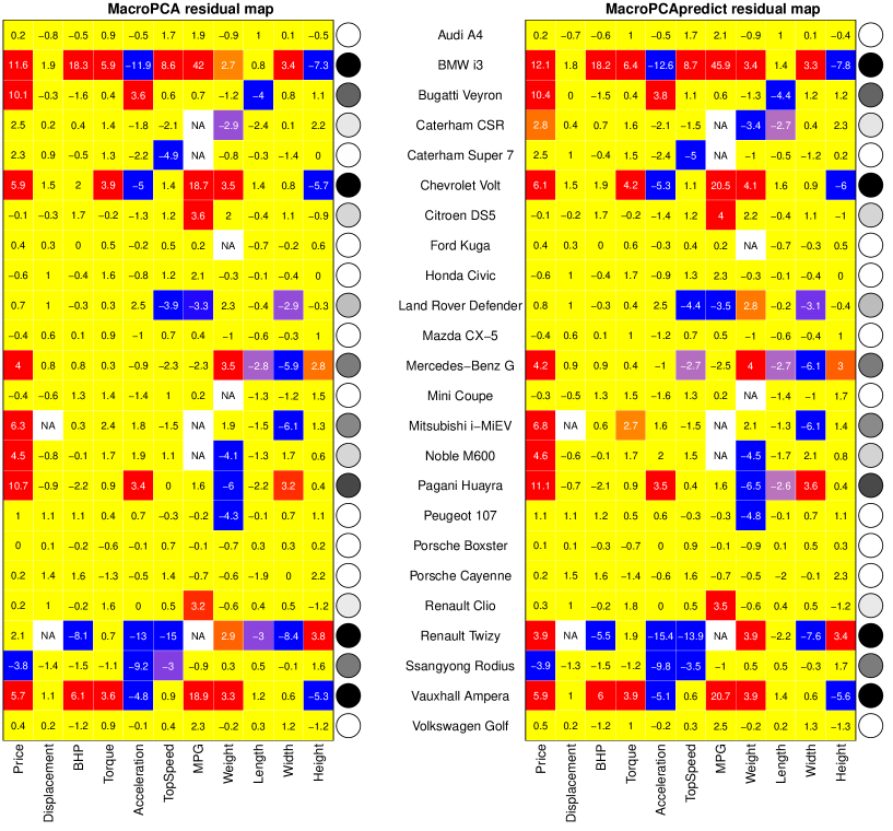
The right hand panel of Figure 3 shows the results of MacroPCA by a modification of the cell map introduced by Rousseeuw and Van den Bossche (2018). The computations were performed on all 297 cars, but in order to make the map fit on a page it only shows 24 cars, including some of the more eventful cases. The color of the cells stems from the standardized residual matrix obtained by MacroPCA. Cells with are considered regular and colored yellow in the residual map, whereas the missing values are white. Outlying residuals receive a color which ranges from light orange to red when and from light purple to dark blue when . So a dark red cell indicates that its observed value is much higher than its fitted value, while a dark blue cell means the opposite.
To the right of each row in the map is a circle whose color varies from white to black according to the orthogonal distance given by (4) compared to the cutoff (3). Cases with lie close to the PCA subspace and receive a white circle. The others are given darker shades of gray up to black according to their .
On these data we also ran the ICPCA method, which handles missing values in classical PCA. It differs from MacroPCA in some important ways: the initial imputations are by nonrobust column means, the iterations carry out CPCA and do not exclude outlying rows, and the residuals are standardized by the nonrobust standard deviation. By itself ICPCA does not provide a residual map, but we can construct one anyway by plotting the nonrobust standardized residuals with the same color scheme, yielding the left panel of Figure 3.
The ICPCA algorithm finds high orthogonal distances (dark circles) for the BMW i3, the Chevrolet Volt, the Renault Twizzy and the Vauxhall Ampera. These are hybrid or purely electrical cars with a high or missing MPG (miles per gallon). Note that the Ssangyong Rodius and Renault Twizzy get blue cells for their acceleration time of zero seconds, which is physically impossible.
On this dataset the ICPCA algorithm provides decent results because the total number of outliers is small compared to the size of the data, and indeed the residual map of all 297 cars was mostly yellow. But MacroPCA (right panel) detects more deviating behavior. The orthogonal distance of the hybrid Citroen DS5 and the electrical Mitsubishi i-MiEV are now on the high side, and the method flags the Bugatti Veyron and Pagani Huayra supercars as well as the Land Rover Defender and Mercedes-Benz G all-terrain vehicles. It also flags more cells, giving a more complete picture of the special characteristics of some cars.
 |
 |
We can also compute the score distance of each case, which is the robustified Mahalanobis distance of its projection on the PCA subspace among all such projected points. It is easily computed as
| (5) |
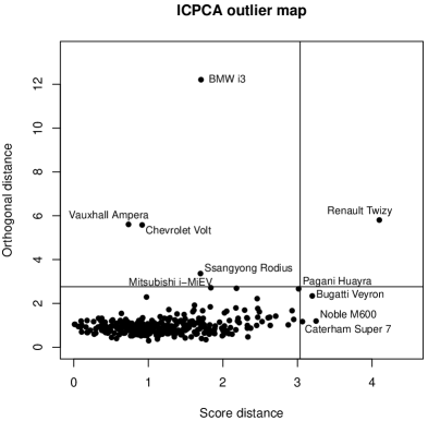
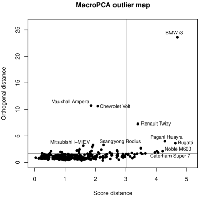
where are the scores and the eigenvalues obtained by MacroPCA. This allows us to construct a PCA outlier map of cases as introduced in Hubert et al. (2005), which plots the orthogonal distances on the vertical axis versus the score distances . The MacroPCA outlier map of these data is the right panel of Figure 4. The vertical line indicates the cutoff and the horizontal line is the cutoff .
Regular cases are those with a small and a small . Cases with large and small are called good leverage points. The cases with large can be divided into orthogonal outliers (when their is small) and bad leverage points (when their is large too). We see several orthogonal outliers such as the Vauxhall Ampera as well as some bad leverage points, especially the BMW i3. There are also some good leverage points.
The left panel displays the outlier map for ICPCA. It flags the BMW i3 as an orthogonal outlier. This behavior is typical because a bad leverage point will attract the fit of classical methods, making it appear less special. For the same reason ICPCA considers some of the good leverage points as regular cases. That the ICPCA outlier map is still able to flag some outliers is due to the fact that this dataset only has a small percentage of outlying rows.
4 Online data analysis
Applying MacroPCA to a data set yields a PCA fit. Now suppose that a new case (row) comes in, and we would like to impute its missing values, detect its outlying cells and impute them, estimate its scores, and find out whether it is a rowwise outlier. We could of course append to and rerun MacroPCA, but that would be very inefficient.
Instead we propose a method to analyze using only the output of MacroPCA on the initial set . This can be done quite fast, which makes the procedure suitable for online process control. For outlier-free data with NA’s this was studied by Nelson et al. (1996) and Walczak and Massart (2001). Folch-Fortuny et al. (2015) call this model exploitation, as opposed to model building (fitting a PCA model). Our procedure consists of two stages, along the lines of MacroPCA.
-
1.
DDCpredict is a new function which only uses and the output of DDC on the initial data . First the entries of are standardized using the robust location and scale estimates from DDC. Then all with are replaced by NA’s. Next all NA’s are estimated as in DDC making use of the pre-built coefficients and weights . Also the deshrinkage step uses the original robust slopes. The DDCpredict stage yields the imputed vector and the standardized residual of each cell .
-
2.
MacroPCApredict improves on the initial imputation . The improvements are based solely on the and that were obtained by MacroPCA on the original data . Step is of the following form:
-
(a)
Project the imputed case on the MacroPCA subspace to obtain its scores vector ;
-
(b)
transform the scores to the original space, yielding ;
-
(c)
Reimpute the outlying cells and missing values of by the corresponding values of , yielding .
These steps are iterated until convergence (when the new imputed values are within a tolerance of the old ones) or the maximal number of steps (by default 20) is reached. We denote the final as .
Next we create by replacing the missing values in by the corresponding cells in . We then compute the orthogonal distance and the score distance . If the new case is flagged as an orthogonal outlier. Finally the cell residuals are standardized as in the last step of MacroPCA, and used to flag outlying cells in .
-
(a)
To illustrate this prediction procedure we re-analyze the Top Gear data set. We exclude the 24 cars shown in the residual map of Figure 3 and build the MacroPCA model on the remaining data. This model was then provided to analyze the 24 selected cars as ‘new’ data. Figure 5 shows the result. As before the cells are colored according to their standardized residual, and the circles on the right are filled according to their . The left panel is the MacroPCA residual map shown in Figure 3, which was obtained by applying MacroPCA to the entire data set. The right panel shows the result of analyzing these 24 cases using the fit obtained without them. The residual maps are quite similar. Note that each cell now shows its standardized residual (instead of its data value as in Figure 3), making it easier to see the differences.
5 Simulations
We have compared the performance of ICPCA, MROBPCA and MacroPCA in an extensive simulation study. Several contamination models were considered with missing values, cellwise outliers, rowwise outliers, and combinations of them. Only a few of the results are reported here since the others yielded similar conclusions.
The clean data are generated from a multivariate Gaussian with and two types of covariance matrices . The first one is based on the structured correlation matrix called A09 where each off-diagonal entry is . The second type of covariance matrix is based on the random correlation matrices of Agostinelli et al. (2015) and will be called ALYZ. These correlation matrices are turned into covariance matrices with other eigenvalues. More specifically, the diagonal elements of the matrix from the spectral decomposition are replaced by the desired values listed below. The specifications of the clean data are , , and (since ). MacroPCA takes less than a second for , as seen in Figure 2.
In a first simulation setting, the clean data are modified by replacing a random subset of 5%, 10%, … up to 30% of the cells with NA’s. The second simulation setting generates NA’s and outlying cells by randomly replacing 20% of the cells by missing values and 20% by the value where is the -th diagonal element of and ranges from 0 to 20. The third simulation setting generates NA’s and outlying rows. Here 20% of random cells are replaced by NA’s and a random subset of 20% of the rows is replaced by rows generated from where varies from 0 to 50 and is the th eigenvector of . The last simulation setting generates 20% of NA’s, together with 10% of cellwise outliers and 10% of rowwise outliers in the same way.
In each setting we consider the set C consisting of the rows that were not replaced by rowwise outliers, with , and the data matrix consisting of those rows of the clean data . As a baseline for the simulation we apply classical PCA to and denote the resulting predictions by for in . We then measure the mean squared error (MSE) from the baseline:
where is the predicted value for obtained by applying the different methods to the contaminated data. The MSE is then averaged over 100 replications.
| A09, fraction of missing values | ALYZ, fraction of missing values |
|---|---|
 |
 |
Figure 6 shows the performance of ICPCA, MROBPCA and MacroPCA when some data becomes missing. As CPCA and ROBPCA cannot deal with NA’s, they are not included in this comparison. Since there are no outliers the classical ICPCA performs best, followed by MROBPCA and MacroPCA which perform similarly to each other, and only slightly worse than ICPCA considering the scale of the vertical axis which is much smaller than in the other three simulation settings.
| A09, missing values & cellwise | ALYZ, missing values & cellwise |
|---|---|
 |
 |
Now we set 20% of the data cells to missing and add 20% of cellwise contamination given by . Figure 7 shows the performance of ICPCA, MROBPCA and MacroPCA in this situation. The MSE of both ICPCA and MROBPCA grows very fast with which indicates that these methods are not at all robust to cellwise outliers. Note that so on average of the rows are contaminated, whereas no purely rowwise method can handle more than 50%. MacroPCA is the only method that can withstand cellwise outliers here. When is smaller than 5 the MSE goes up, but this is not surprising as in that case the values in the contaminated cells are still close to the clean ones. As soon as the contamination is sufficiently far away, the MSE drops to a very low value.
| A09, missing values & rowwise | ALYZ, missing values & rowwise |
|---|---|
 |
 |
Figure 8 presents the results of ICPCA, MROBPCA and MacroPCA when there are 20% of missing values combined with 20% of rowwise contamination. As expected, the ICPCA algorithm breaks down while MROBPCA and MacroPCA provide very good results. MROBPCA and MacroPCA are affected the most (but not much) by nearby outliers, and very little by far contamination.
| A09, missing & cellwise & rowwise | ALYZ, missing & cellwise & rowwise |
|---|---|
 |
 |
Finally, Figure 9 presents the results in the situation of 20% of missing values combined with 10% of cellwise and 10% of rowwise contamination. In this scenario the ICPCA and MROBPCA algorithms break down whereas MacroPCA still provides reasonable results.
In this section the missing values were generated in a rather simple way. In Section A.3 they are generated in a more challenging way but still MAR, with qualitatively similar results.
6 Real data examples
6.1 Glass data
The glass dataset (Lemberge et al., 2000) contains spectra with wavelengths of archeological glass samples. It is available in the R package cellWise (Raymaekers et al., 2018). The MacroPCA method selects 4 principal components and yields a matrix of standardized residuals. There is not enough resolution on a page to show so many individual cells in a residual map. Therefore we created a map (the top panel of Figure 10) which combines the residuals into blocks of cells. The color of each block now depends on the most frequent type of outlying cell in it, the resulting color being an average. For example, an orange block indicates that quite a few cells in the block were red and most of the others were yellow. The more red cells in the block, the darker red the block will be. We see that MacroPCA has flagged a lot of cells, that happen to be concentrated in a minority of the rows where they show patterns. In fact, the colors indicate that some of the glass samples (between 22 and 30) have a higher concentration of phosphor, whereas rows 57–63 and 74–76 had an unusually high concentration of calcium. The bottom part of the residual map looks very different, due to the fact that the measuring instrument was cleaned before recording the last 38 spectra. One could say that those outlying rows belong to a different population.
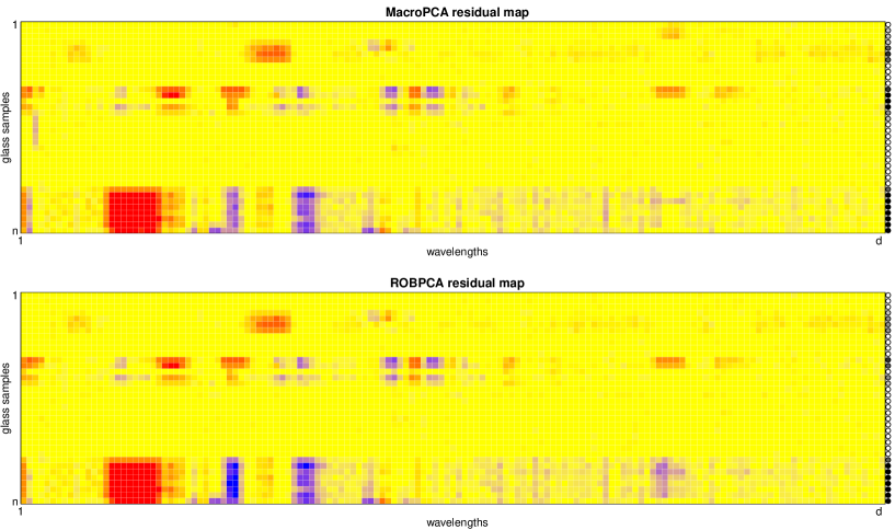
Since the dataset has no NA’s and we found that fewer than half of the rows are outlying, it can also be analyzed by the original ROBPCA method as was done by Hubert et al. (2005), also for . This detects the same rowwise outliers. In principle ROBPCA is a purely rowwise method that does not flag cells. Even though ROBPCA does not produce a residual map, we can construct one analogously to that of MacroPCA. First we construct the residual matrix of ROBPCA, the rows of which are given by where is the projection of on the ROBPCA subspace. We then standardize the residuals in each column by dividing them by a robust 1-step scale M-estimate. This yields the bottom panel of Figure 10. We see that the two residual maps look quite similar.
This example illustrates that purely rowwise robust methods can be useful to detect cellwise outliers when these cells occur in fewer than 50% of the rows. But if the cellwise outliers contaminate more rows, this approach is insufficient.
6.2 DPOSS data
In our last example we analyze data from the Digitized Palomar Sky Survey (DPOSS) described by Odewahn et al. (1998). This is a huge database of celestial objects, from which we have drawn 20,000 stars at random. Each star has been observed in the color bands J, F, and N. Each band has 7 variables. Three of them measure light intensity: for the J band they are MAperJ, MTotJ and MCoreJ where the last letter indicates the band. The variable AreaJ is the size of the star based on its number of pixels. The remaining variables IR2J, csfJ and EllipJ combine size and shape. (There were two more variables in the original data, but these measured the background rather than the star itself.) There are substantial correlations between these 21 variables.
 |
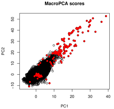 |
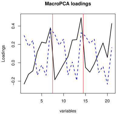
In this dataset 84.6% of the rows contain NA’s (in all there are 50.2% missing entries.) Often an entire color band is missing, and sometimes two. We applied MacroPCA to these data, choosing components according to the scree plot. The left panel of Figure 11 shows the loadings of the first and second component. It appears that the first component captures the overall negative correlation between two groups of variables: those measuring light intensity (the first 3 variables in each band) and the others (variables 4 to 7 in each band). The right panel is the corresponding scores plot, in which the 150 stars with the highest orthogonal distance are shown in red. Most of these stand out in the space of PC1 and PC2 (bad leverage points), whereas some only have a high (orthogonal outliers).
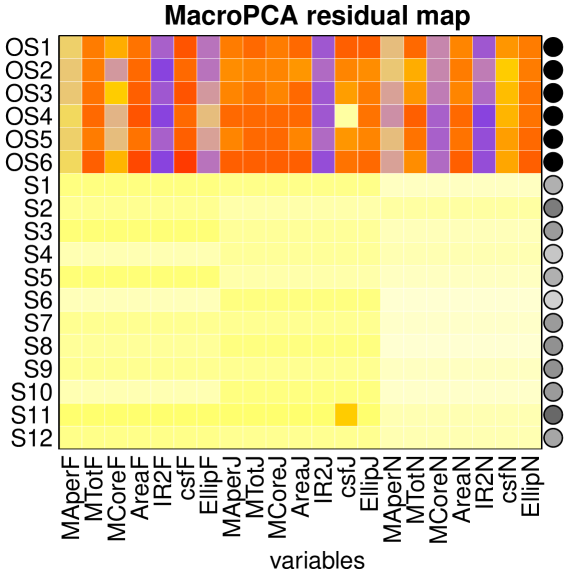
Figure 12 shows the residual map of MacroPCA, in which each row block combines 25 stars. The six rows at the top correspond to the 150 stars with highest . We note that the outliers tend to be more luminous (MTot) than expected and have a larger Area, which suggests giant stars. The analogous residual map of ICPCA (not shown) did not reveal much. Note that the non-outlying rows in the bottom part of the residual map are yellow, and the missing color bands show up as blocks in lighter yellow (a combination of yellow and white cells).
7 Conclusions
The MacroPCA method is able to handle missing values, cellwise outliers, and rowwise outliers. This makes it well-suited for the analysis of possibly messy real data. Simulation showed that its performance is similar to a classical method in the case of outlier-free data with missing values, and to an existing robust method when the data only has rowwise outliers. The algorithm is fast enough to deal with many variables, and we intend to speed it up by recoding it in C.
MacroPCA can analyze new data as they come in, only making use of its existing output obtained from the initial dataset. It imputes missing values in the new data, flags and imputes outlying cells, and flags outlying rows. This computation is fast, so it can be used to screen new data in quality control or even online process control. (One can update the initial fit offline from time to time.) The advantage of MacroPCA is that it not only tells us when the process goes out of control, but also which variables are responsible.
Potential extensions of MacroPCA include methods of PCA regression and partial least squares able to deal with rowwise and cellwise outliers and missing values.
8 Software Availability
The R code of MacroPCA, as well as the data sets and an example script, are available at https://wis.kuleuven.be/stat/robust/software. It will be incorporated in the R package cellWise on CRAN.
Appendix A Appendix
A.1 Example illustrating step 5 of MacroPCA
Steps 1 to 4 of the MacroPCA algorithm construct a robust -dimensional subspace. The purpose of step 5 is to robustly estimate basis vectors (loadings) of the subspace. The columns of the loadings matrix from step 4 need not be robust, because some of the rows in might be outlying inside the subspace. Such points are called good leverage points, where ‘good’ refers to the fact that they do not harm the estimation of the subspace, but on the other hand they can affect the estimated eigenvectors and eigenvalues. We illustrate this by a small toy example.
A clean data set with and was generated according to a trivariate Gaussian distribution, with covariance matrix chosen in such a way that components explain 90% of the total variance. Next, the data was contaminated by replacing 20% of the points by good leverage points. This means that these points are only outlying inside the two-dimensional subspace, and not in the direction of its orthogonal complement.
| With step 5 | Without step 5 |
|---|---|
 |
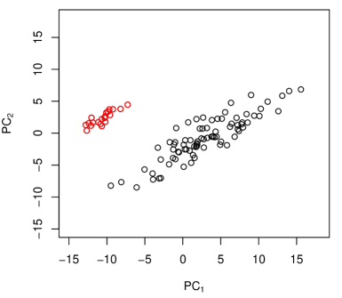 |
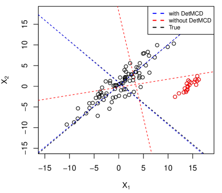
Figure 13 shows the scatter plot of the data points projected on this two-dimensional subspace. The black dashed lines represent the eigenvectors of the clean data, and the blue and red dashed lines are the estimated eigenvectors of MacroPCA on the contaminated data, with and without step 5. The center and directions of the blue lines were obtained by DetMCD in step 5, whereas the red lines correspond to the center and the loading matrix obtained in step 4. The blue lines (with step 5) are almost on top of the black ones, whereas the red lines (without step 5) are very different. Although the blue and the red fits span the same subspace, we see that without step 5 the estimated loading vectors are far off.
This can also be seen in Figure 14 which shows the scores on the first two components of MacroPCA with and without step 5. In the left panel we see that the scores reflect the shape of the clean data, whereas those in the right panel were affected by the leverage points. This illustrates that the interpretation of the results can be distorted by good leverage points if step 5 is not taken.
A.2 Computational complexity of MacroPCA
The computational complexity of MacroPCA depends on how its steps are implemented. The DDC in the first part has an implementation (Raymaekers et al., 2018). The outlyingness (2) in step 1 requires time. The classical PCA in steps 2, 3, and 4 needs if it is carried out by singular value decomposition (SVD) instead of the eigendecomposition of a covariance matrix. The scores and predictions in steps 3, 4 and 6 require but since we assume that the number of components is at most 10 this becomes . The DetMCD in step 5 combines initial estimators of total complexity with C-steps that require if performed by SVD. The robust scales of the residuals in step 6 take time. The overall complexity of MacroPCA thus becomes which is not much higher than the of classical PCA.

A.3 Generating NA’s by a different MAR mechanism
In this paper we have assumed that the missingness mechanism is MAR (missing at random), a typical assumption underlying EM-based methods such as ICPCA and MROBPCA that are incorporated in MacroPCA. MAR says that the missingness of a cell is unrelated to the value the cell would have had, but may be related to the values of other cells in the same row; see, e.g., Schafer and Graham (2002).
In the simulations of Section 5 a random subset of of the cells was replaced by NA’s. This is a simple special case of MAR, in fact it is MCAR (missing completely at random) which assumes that the missingness of a cell does not depend on its own value or that of any other cell in its row.
Here we will look at a more challenging mechanism that is still MAR but no longer MCAR. Many MAR mechanisms are possible. We chose the following one where the positions of the NA’s clearly depend on the values of the other cells. Given the uncontaminated matrix we first construct the matrix with cell values
Next, the cells of corresponding to the highest values of are set to missing. Other than this, the simulation setup is as described in Section 5.
| A09, fraction of missing values | ALYZ, fraction of missing values |
|---|---|
 |
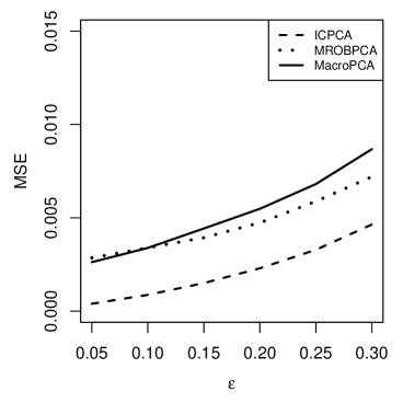 |
The simulation results of ICPCA, MROBPCA and MacroPCA are shown in Figure 16. Compared to the results with MCAR missing values in Figure 6 we see that the shape of the plots is very similar, only the scale of the MSE values is increased but it remains very low.
Next, the other three settings in Section 5 were repeated with MAR missing values. This yielded Figures 17, 18 and 19, which are extremely similar to the corresponding Figures 7, 8 and 9. This confirms the suitability of MacroPCA in the MAR setting.
| A09, missing values & cellwise | ALYZ, missing values & cellwise |
|---|---|
 |
 |
| A09, missing values & rowwise | ALYZ, missing values & rowwise |
|---|---|
 |
 |
| A09, missing & cellwise & rowwise | ALYZ, missing & cellwise & rowwise |
|---|---|
 |
 |
A.4 Simulation with data resembling DPOSS
The DPOSS data analyzed in Subsection 6.2 has many NA’s, in fact 50% of the cells are missing. The simulation study of Section 5 did not include such an extreme situation. In order to check whether MacroPCA can handle data with these characteristics, we redid the simulation leading to Figure 9 for variables and 50% of missing values as well as 5% of cellwise outliers and 5% of rowwise outliers, all as in the DPOSS data.
| A09, missing & cellwise & rowwise | ALYZ, missing & cellwise & rowwise |
|---|---|
 |
 |
Figure 20 shows the results, which indicate that ICPCA and MROBPCA broke down whereas MacroPCA still worked well.
Acknowledgments. The research of P. Rousseeuw has been supported by projects of Internal Funds KU Leuven. W. Van den Bossche obtained financial support from the EU Horizon 2020 project SCISSOR: Security in trusted SCADA and smart-grids 2015-2018. The reviewers provided helpful suggestions to improve the presentation.
Supplementary Material. This is a text with more details about the first part of the MacroPCA algorithm and a list of notations.
References
- Agostinelli et al. (2015) Agostinelli, C., A. Leung, V. J. Yohai, and R. H. Zamar (2015). Robust estimation of multivariate location and scatter in the presence of cellwise and casewise contamination. Test 24, 441–461.
- Alfons (2016) Alfons, A. (2016). robustHD: Robust methods for high-dimensional data. CRAN. R package version 0.5.1.
- Alqallaf et al. (2009) Alqallaf, F., S. Van Aelst, V. J. Yohai, and R. H. Zamar (2009). Propagation of outliers in multivariate data. The Annals of Statistics 37, 311–331.
- Cheng and Victoria-Feser (2002) Cheng, T.-C. and M.-P. Victoria-Feser (2002). High breakdown estimation of multivariate location and scale with missing observations. British Journal of Mathematical and Statistical Psychology 55, 317–335.
- Croux and Ruiz-Gazen (2005) Croux, C. and A. Ruiz-Gazen (2005). High breakdown estimators for principal components: the projection-pursuit approach revisited. Journal of Multivariate Analysis 95, 206–226.
- Danilov et al. (2012) Danilov, M., V. J. Yohai, and R. H. Zamar (2012). Robust estimation of multivariate location and scatter in the presence of missing data. Journal of the American Statistical Association 107, 1178–1186.
- Engelen et al. (2005) Engelen, S., M. Hubert, and K. Vanden Branden (2005). A comparison of three procedures for robust PCA in high dimensions. Austrian Journal of Statistics 34, 117–126.
- Folch-Fortuny et al. (2015) Folch-Fortuny, A., F. Arteaga, and A. Ferrer (2015). PCA model building with missing data: New proposals and a comparative study. Chemometrics and Intelligent Laboratory Systems 146, 77–88.
- Hubert et al. (2005) Hubert, M., P. J. Rousseeuw, and K. Vanden Branden (2005). ROBPCA: a new approach to robust principal components analysis. Technometrics 47, 64–79.
- Hubert et al. (2002) Hubert, M., P. J. Rousseeuw, and S. Verboven (2002). A fast robust method for principal components with applications to chemometrics. Chemometrics and Intelligent Laboratory Systems 60, 101–111.
- Hubert et al. (2012) Hubert, M., P. J. Rousseeuw, and T. Verdonck (2012). A deterministic algorithm for robust location and scatter. Journal of Computational and Graphical Statistics 21, 618–637.
- Kiers (1997) Kiers, H. (1997). Weighted least squares fitting using ordinary least squares algorithms. Psychometrika 62, 251–261.
- Krzanowski (1979) Krzanowski, W. (1979). Between-groups comparison of principal components. Journal of the American Statistical Association 74, 703–707.
- Lemberge et al. (2000) Lemberge, P., I. De Raedt, K. Janssens, F. Wei, and P. J. Van Espen (2000). Quantitative Z-analysis of 16th–17th century archaelogical glass vessels using PLS regression of EPXMA and -XRF data. Journal of Chemometrics 14, 751–763.
- Locantore et al. (1999) Locantore, N., J. Marron, D. Simpson, N. Tripoli, J. Zhang, and K. Cohen (1999). Robust principal component analysis for functional data. Test 8, 1–73.
- Lopuhaä and Rousseeuw (1991) Lopuhaä, H. and P. J. Rousseeuw (1991). Breakdown points of affine equivariant estimators of multivariate location and covariance matrices. The Annals of Statistics 19, 229–248.
- Maronna (2005) Maronna, R. (2005). Principal components and orthogonal regression based on robust scales. Technometrics 47, 264–273.
- Nelson et al. (1996) Nelson, P., P. Taylor, and J. MacGregor (1996). Missing data methods in PCA and PLS: Score calculations with incomplete observations. Chemometrics and Intelligent Laboratory Systems 35, 45–65.
- Odewahn et al. (1998) Odewahn, S., S. Djorgovski, R. Brunner, and R. Gal (1998). Data From the Digitized Palomar Sky Survey. Technical report, California Institute of Technology.
- Raymaekers et al. (2018) Raymaekers, J., P. J. Rousseeuw, and W. Van den Bossche (2018). cellWise: Analyzing Data with Cellwise Outliers. CRAN. R package version 2.0.8.
- Rousseeuw and Hubert (2018) Rousseeuw, P. J. and M. Hubert (2018). Anomaly detection by robust statistics. WIREs Data Mining and Knowledge Discovery e1236, 1–14.
- Rousseeuw and Leroy (1987) Rousseeuw, P. J. and A. Leroy (1987). Robust Regression and Outlier Detection. New York: Wiley-Interscience.
- Rousseeuw and Van den Bossche (2018) Rousseeuw, P. J. and W. Van den Bossche (2018). Detecting deviating data cells. Technometrics 60, 135–145.
- Schafer and Graham (2002) Schafer, J. and J. Graham (2002). Missing data: Our view of the state of the art. Psychological Methods 7, 147–177.
- Serneels and Verdonck (2008) Serneels, S. and T. Verdonck (2008). Principal component analysis for data containing outliers and missing elements. Computational Statistics & Data Analysis 52, 1712–1727.
- Van Aelst et al. (2012) Van Aelst, S., E. Vandervieren, and G. Willems (2012). A Stahel-Donoho estimator based on Huberized outlyingness. Computational Statistics & Data Analysis 56, 531–542.
- Walczak and Massart (2001) Walczak, B. and D. Massart (2001). Tutorial: Dealing with missing data, part I. Chemometrics and Intelligent Laboratory Systems 58, 15–27.
Supplementary Material
1. Description of the DDC algorithm
Here we summarize the steps of the DDC algorithm, and refer to Rousseeuw and Van den Bossche (2018) for more details.
-
1.
Standardization. The location and scale estimates of each column of are calculated as and where robLoc and robScale are 1-step M-estimators of location and scale. Then is standardized by column to by .
-
2.
Univariate outlier detection. An initial cellwise outlier detection is performed by flagging cells that are outlying in their column. To this end a new matrix is created in which univariate cellwise outliers are replaced by missing values, i.e. contains the entries
where the cutoff value is set to with probability by default.
-
3.
Bivariate relations. To reduce the propagation effect of cellwise outliers, only bivariate relations are considered. For any two columns of we calculate where robCorr is a robust correlation measure that discards missing values. Variables that satisfy for some are called connected while the others are called standalone variables.
The connected variables are sufficiently correlated to help predict each other. To this end we compute the robust slopes of the connected variables as where robSlope robustly estimates the slope of a no-intercept regression line that predicts variable from variable . Also the function robSlope discards missing values.
-
4.
Prediction. A crucial aspect of the DDC algorithm is its ability to robustly predict cell values. For the standalone variables all univariately outlying are predicted by zero, since no further information is available. (This means the unstandardized are replaced by the robust location estimate .) The non-outlying cell values are are predicted by themselves. The prediction of a connected variable is more involved. In words, for such a variable a set of ‘simple’ predictions is made, each using the slope of a variable to which it is connected. The final predictions are obtained by combining these simple predictions, using the correlations of the connected variables as weights.
More formally, for each variable the set is considered which consists of all variables with , including itself. Next, for all and the predicted values are calculated as
(S.1) where . The weighted average is taken over all for which is not missing. Any missing value in is set to zero. Note that for standalone variables since .
-
5.
Deshrinkage. Let us consider a column . The predictions typically have a smaller scale than that of the original column of . To compensate for this shrinkage, is replaced by where
-
6.
Flagging cellwise outliers. The final predictions can be used to flag cellwise outliers. Any cell whose value differs too much from its prediction value is flagged. More precisely, the standardized cell residuals
(S.2) are computed for all non-missing and all cells with are flagged. Their indices (positions) are stored in a set .
-
7.
Flagging rowwise outliers. The DDC method can also flag some outlying rows based on the standardized cell residuals . For multivariate Gaussian data without outliers so the cdf of is approximately the cdf of . This motivates the criterion
(S.3) Next, the are standardized robustly and the rows for which the squared standardized exceeds the cutoff are flagged and stored in a set .
-
8.
Imputation. The NA-imputed matrix is assembled by replacing all missing values of the original matrix with their predictions. The more fully imputed matrix also replaces all cellwise outliers, i.e.
These imputed matrices are turned into imputed matrices and by undoing the standardization.
Table S.1 lists all matrices, vectors and index sets used in this first stage of MacroPCA. The DDC algorithm has been implemented as the function DetectDeviatingCells in the R package cellWise (Raymaekers et al., 2018) available in CRAN.
Table S.1: Overview of notations used in the DDC
stage of MacroPCA
original data matrix,
with rows
standardized data matrix
standardized data matrix with
univariate outliers set to NA
matrix with predicted values for
standardized residual matrix
set of cells flagged as cellwise
outliers
measure of rowwise outlyingness based
on
set of rows flagged as possible rowwise
outliers, based on
NA-imputed standardized data: all missing
cells replaced by
predicted values
imputed standardized data matrix: all
cells in and all
missing values imputed
NA-imputed data matrix,
with rows
imputed data matrix (all missing values
and all flagged cells are
imputed), with rows
2. Notations used in MacroPCA
The notations used in the second part of the MacroPCA algorithm are listed in Table S.2.
Table S.2: Overview of notations used in the second
stage of MacroPCA
initial cell-imputed data matrix,
with rows
index set of the rows with smallest
outlyingness
dimension of the PCA subspace
PCA estimates from iteration step ,
based on the imputed
rows in
NA-imputed matrix (all missing
cells imputed),
with rows
cell-imputed matrix (imputes
outlying cells in rows of
and all missing values),
with rows
prediction for based
on and
,
with rows
scores of with respect
to and
orthogonal distance of with
respect to the current PCA
subspace
index set of the rows with small
enough
cell-imputed data matrix at the end of
the algorithm, with
rows
center and PCA loadings of
scores of the rows in
with respect to
and
robust center and loadings
of
center and loadings of the final
PCA fit
scores of all rows of
with respect to the final
PCA fit
predicted values of all rows
of ,
with rows
scores of all rows of with
respect to the final PCA fit
orthogonal distance of with respect
to the final PCA
subspace
final standardized residual matrix of .