Discrete worldline instantons

Abstract

The semiclassical approximation of the worldline path integral is a powerful tool to study nonperturbative electron-positron pair creation in spacetime-dependent background fields. Finding solutions of the classical equations of motion, i.e. worldline instantons, is possible analytically only in special cases, and a numerical treatment is nontrivial as well. We introduce a completely general numerical approach based on an approximate evaluation of the discretized path integral that easily and robustly gives the full semiclassical pair production rate in nontrivial multi-dimensional fields, and apply it to some example cases.

I Introduction

An as of today still experimentally unconfirmed prediction of quantum electrodynamics is that of nonperturbative electron-positron pair creation in the presence of a strong electric field Sauter (1931); Heisenberg and Euler (1936); Hund (1941). Schwinger Schwinger (1951) gave the pair production rate per unit volume $\mathcal{P}_{e^{+}e^{-}}$ (or more properly the rate of vacuum decay Cohen and McGady (2008)) in a constant, homogeneous electric field $E$ in 3+1 dimensions as ($\hbar=c=1$)

$$\mathcal{P}_{e^{+}e^{-}}=\frac{(qE)^{2}}{4\pi^{3}}\sum_{n=1}^{\infty}\frac{1}{n^{2}}\exp\left(-n\pi\frac{m^{2}}{qE}\right),$$ (1)

where $q$ is the elementary charge and $m$ the mass of the electrons and positrons. The generalization to inhomogeneous and time dependent background fields is far from straightforward, since this is a nonperturbative effect (as is visible from the inverse dependence on $q$ and $E$ in the exponent of (1)). Apart from the fundamental interest in this effect as a prototypical example for a nonperturbative phenomenon in quantum field theory, a better understanding is also desirable in view of the various experimental initiatives aimed at reaching ultra-high field strengths .

It is in general difficult to obtain the pair production probability for multi-dimensional fields. While there has recently been some progress Kohlfürst and Alkofer (2016); Aleksandrov et al. (2017); Kohlfürst and Alkofer (2018); Lv et al. (2018); Aleksandrov et al. ; Kohlfürst (2018) in direct numerical computation of the exact probability for multi-dimensional fields, we will instead focus on an approach using the worldline path integral.

This formulation is an alternative to path integrals over fields to express amplitudes in quantum field theories. The first steps in this direction were pioneered by Fock, who expressed solutions of the Dirac equation via a four dimensional Schrödinger-type equation with space and time parameterized by an additional parameter Fock (1937). After Nambu emphasized how beneficial this representation would be in the path integral approach Nambu (1950), Feynman derived the Klein-Gordon propagator Feynman (1950) and Dirac propagator Feynman (1951) in this worldline formulation. In parallel, Schwinger’s famous paper Schwinger (1951) used a similar representation.

It is possible to approximate this worldline path integral for inhomogeneous fields numerically using discretization and Monte Carlo methods Gies and Langfeld (2001); Gies et al. (2003); Gies and Klingmüller (2005); Gies and Roessler (2011). Although our method is based on discretization as well, we use an instanton approach to compute the integrals instead of statistical sampling.

Both Feynman and Schwinger mentioned the four dimensional particle’s equations of motion in the classical limit, but the first explicit mention of an instanton approximation to the (Euclidean) worldline path integral was given by Affleck, Alvarez and Manton Affleck et al. (1982). They derived the pair production rate for a constant homogeneous background field in a way that is very similar to the method used today. The approach was extended to inhomogeneous fields, including the sub-leading fluctuation prefactor Dunne and Schubert (2005); Dunne et al. (2006).

An exact analytic treatment is possible in some simple cases Dunne and Schubert (2005); Dunne et al. (2006); Ilderton et al. (2015) and analytic approximations allows us to study suitable limiting cases Schützhold et al. (2008); Gies and Torgrimsson (2016); Schneider and Schützhold (2016), but in general solutions of the instanton equations of motion have to be found numerically. This can be done using, e.g., shooting methods Dunne and Wang (2006), but the highly nonlinear nature of the equations of motion makes this approach very unstable.

After briefly sketching the semiclassical approximation of the worldline path integral in section II, we introduce a different approach to numerically evaluate the path integral by discretization in sections III and IV, and a method to trace families of solutions over a range of field parameters in section V. Finally, we will apply the method to some example cases, both with results known analytically (to assess the accuracy of the approximation) and new examples to demonstrate the scope of the approach in section VI.

II Worldline instanton method

The central object of the method is the effective action $\Gamma_{\mathrm{M}}$, defined using the vacuum persistence amplitude

$$e^{i\Gamma_{\mathrm{M}}}:=\braket{0_{\mathrm{out}}}{0_{\mathrm{in}}}.$$ (2)

We take the probability for pair creation to be the complement of the vacuum remaining stable, so

$$P^{e^{+}e^{-}}=1-\left|\braket{0_{\mathrm{out}}}{0_{\mathrm{in}}}\right|^{2}=1-\left|e^{i\Gamma_{\mathrm{M}}}\right|^{2}\approx 2\Im\Gamma_{\mathrm{M}},$$ (3)

the subscript _M denoting the physical, Minkowskian quantity. We will work with the Euclidean effective action $\Gamma$, related to the Minkowski expression by $\Gamma_{\mathrm{M}}=i\Gamma$, so $\Im\Gamma_{\mathrm{M}}=\Re\Gamma$ Dunne et al. (2006).

The Euclidean worldline path integral for spinor QED reads (see, e.g., Schubert (2001, 2012))

$$\Gamma= \int_{0}^{\infty}\frac{\mathrm{d}{T}}{T}e^{-\frac{m^{2}}{2}T}\int_{x(T)=x(0)}\mathcal{D}x(\tau)$$

$$\quad\times\Phi[x]\exp\left(-\int_{0}^{T}\mathrm{d}{\tau}\left(\frac{\dot{x}^{2}}{2}+iqA(x)\cdot\dot{x}\right)\right),$$ (4)

where $A_{\mu}$ is the Euclidean potential representing the external electromagnetic field $F_{\mu\nu}$ and $x_{\mu}(\tau)$ are periodic worldlines in Euclidean space parametrized by the “proper time” $\tau$ with $\dot{x}^{\mu}=\mathrm{d}x^{\mu}/\mathrm{d}\tau$. There exist a couple of different representations of the spin factor, see Schubert (2001); Gies and Hämmerling (2005). We will use

$$\Phi[x]=\frac{1}{2}\operatorname{tr}\mathcal{P}e^{\frac{i}{4}\int_{0}^{T}\mathrm{d}{\tau}\sigma_{\mu\nu}qF_{\mu\nu}(x)},$$ (5)

with $\mathcal{P}$ denoting path ordering, $\operatorname{tr}$ the trace over spinor indices and $\sigma_{\mu\nu}$ the commutator of the Dirac matrices

$$\sigma_{\mu\nu}=\frac{1}{2}\left[\gamma_{\mu},\gamma_{\nu}\right].$$ (6)

For simple fields, the Euclidean potential $A_{\mu}$ and field tensor $F_{\mu\nu}$ are purely imaginary, so $iA_{\mu}$ and $iF_{\mu\nu}$ are real.

We immediately introduce dimensionless quantities using some reference field strength $E$, which makes a numerical treatment possible and simplifies the following derivation,

$$\tilde{x}_{\mu}=x_{\mu}\frac{qE}{m},\quad\tilde{F}_{\mu\nu}=F_{\mu\nu}\frac{1}{E},\quad\tilde{A}_{\mu}=\frac{qE}{m}\frac{1}{E}A_{\mu},$$ (7)

and also rescale the integration variable

$$\tilde{T}=qET,\quad u=\frac{1}{T}\tau=\frac{qE}{\tilde{T}}\tau,\quad\curvearrowright\frac{\partial}{\partial u}=\frac{\tilde{T}}{qE}\frac{\partial}{\partial\tau}.$$ (8)

We can now exchange the order of integration,

$$\Gamma= \int_{x(1)=x(0)}\mathcal{D}{x}(u)\int_{0}^{\infty}\mathrm{d}{\tilde{T}}\,\frac{\Phi[\tilde{x}]}{\tilde{T}}$$ (9)

$$\quad\times\exp\left(-\frac{m^{2}}{qE}\left(\frac{\tilde{T}}{2}+\int\limits_{0}^{1}\mathrm{d}{u}\left(\frac{\dot{\tilde{x}}^{2}}{2\tilde{T}}+i\dot{\tilde{x}}\cdot\tilde{A}\right)\right)\right),$$

so we can perform the $\tilde{T}$-integration using Laplace’s method. Due to our rescaling, $m^{2}/qE$ is singled out as the large parameter of the expansion, while all other quantities are of order unity. We obtain the saddle point $\tilde{T}_{0}=\sqrt{\int_{0}^{1}\mathrm{d}{u}\ \dot{\tilde{x}}^{2}}=:a[\tilde{x}]$, so including the quadratic fluctuation around the saddle we arrive at the approximation

$$\Gamma\approx\int_{x(T)=x(0)}\mathcal{D}{x}(\tau)\sqrt{\frac{2\pi}{a[\tilde{x}]}\frac{qE}{m^{2}}}\Phi[\tilde{x}]e^{-\frac{m^{2}}{qE}\mathcal{A}[\tilde{x}]},$$ (10)

with the non-local (due to $a[\tilde{x}]$) action

$$\mathcal{A}[\tilde{x}]=a[\tilde{x}]+\int\limits_{0}^{1}\mathrm{d}{u}\ \dot{\tilde{x}}\cdot i\tilde{A}(\tilde{x}),$$ (11)

and the spin factor

$$\Phi[\tilde{x}]=\frac{1}{2}\operatorname{tr}\mathcal{P}\exp\left({\frac{a[\tilde{x}]}{4}\int_{0}^{1}\mathrm{d}{u}\ \sigma_{\mu\nu}i\tilde{F}_{\mu\nu}(\tilde{x})}\right).$$ (12)

Note that in (10) we symbolically restored the original parametrization $\mathcal{D}{x}(\tau)$ in the path integral differential, this will be relevant for the discretization in the next section.

Applying Laplace’s method to the path integral, we need to find a path $\tilde{x}_{\mu}(u)$ that satisfies the periodic boundary conditions and extremizes the exponent in (10), so a solution to the Euler-Lagrange equations (the Lorentz force equation in this case)

$$\frac{\ddot{\tilde{x}}_{\mu}}{a[\tilde{x}]}=iq\tilde{F}_{\mu\nu}\dot{\tilde{x}}_{\nu}.$$ (13)

Contracting (13) with $\dot{\tilde{x}}_{\mu}$ we see that (due to the antisymmetry of $\tilde{F}_{\mu\nu}$) $\dot{\tilde{x}}^{2}=\text{const.}=a^{2}$, simplifying the instanton equations of motion to

$$\ddot{\tilde{x}}_{\mu}=iaq\tilde{F}_{\mu\nu}\dot{\tilde{x}}_{\nu}.$$ (14)

The prefactor of the Laplace approximation is given by the second variation of the action around the classical solution to (14), amounting to an operator determinant. The determinant has to be defined carefully, but we can completely sidestep this complication by instead performing Laplace’s method after discretization, when we can calculate the fluctuation prefactor by standard methods of linear algebra.

III Discretization

We approximate (10) by discretizing the trajectories $\tilde{x}_{\mu}(u)$ into $N$ $d$-dimensional points (in general $d=3+1$, but for simple field configurations it is possible to only consider $d=1+1$ or $d=2+1$ dimensions, so we will keep the dimensionality variable):

$$\tilde{x}_{\mu}^{i}\mathrel{\vbox{\hbox{\scriptsize.}\hbox{\scriptsize.}}}=\tilde{x}_{\mu}\left(\frac{l}{N}\right),\quad l=0,1,\dots,N-1.$$ (15)

The velocity is then approximated using (forward) finite differences

$$\dot{\tilde{x}}_{\mu}^{l}\approx\frac{\tilde{x}_{\mu}^{l+1}-\tilde{x}_{\mu}^{l}}{\varepsilon},\quad\varepsilon=\frac{1}{N},$$ (16)

with the identification $\tilde{x}_{\mu}^{N}\equiv\tilde{x}_{\mu}^{0}$.

Discretizing the path integral requires a normalization factor for each $\tilde{x}_{\mu}^{i}$-integral. We could find these factors by performing the integration in the free case, however this is not necessary: In the derivation of (II) the path integral arises as an ordinary nonrelativistic transition amplitude, so we can use Feynman’s normalization $1/A$ for each integral (see, e.g., Feynman (1948)), with

$$A=\sqrt{\frac{2\pi T_{0}}{N}}=\sqrt{\frac{2\pi a[x]}{qEN}}.$$ (17)

Using this normalization and replacing the $N\times d$ integrations by the dimensionless versions we arrive at the discretized worldline path integral

$$\Gamma\approx \left(\prod_{k=0}^{N-1}\int\mathrm{d}{{}^{d}\tilde{x}^{k}}\right)\left(\frac{m^{2}}{qE}\frac{N}{2\pi a[\tilde{x}_{\mu}^{l}]}\right)^{Nd/2}$$

$$\qquad\times\sqrt{\frac{2\pi}{a[\tilde{x}_{\mu}^{l}]}\frac{qE}{m^{2}}}\Phi[\tilde{x}_{\mu}^{l}]e^{-\frac{m^{2}}{qE}\mathcal{A}[\tilde{x}_{\mu}^{l}]}.$$ (18)

As we have now expressed everything in terms of the dimensionless variables, we will from now on drop the tilde. We still need discretized expressions for $a$, $\mathcal{A}$ and $\Phi$,

$$a[x_{\mu}^{l}] \mathrel{\vbox{\hbox{\scriptsize.}\hbox{\scriptsize.}}}=\sqrt{N\sum_{k=0}^{N-1}(x_{\nu}^{k+1}-x_{\nu}^{k})^{2}}$$ (19)

$$\mathcal{A}[x_{\mu}^{l}] \mathrel{\vbox{\hbox{\scriptsize.}\hbox{\scriptsize.}}}=a[x_{\mu}^{l}]$$

$$+\sum_{k=0}^{N-1}\left(\frac{A_{\nu}(x_{\mu}^{k+1})+A_{\nu}(x_{\mu}^{k})}{2}\right)(x_{\nu}^{k+1}-x_{\nu}^{k}),$$ (20)

the square brackets denoting dependence on all points, instead of a particular choice of indices.

The form of discretization of the gauge term is not at all obvious, other choices like having just $A_{\nu}(x_{\mu}^{k})$ or $A_{\nu}(x_{\mu}^{k+1})$ or evaluating the gauge field between points $A_{\nu}((x_{\mu}^{k}+x_{\mu}^{k+1})/2)$ would yield the same classical continuum limit. That does not mean however that the resulting propagator is the same, see Rabello and Farina (1995); Stone (2000); Gaveau et al. (2004); Schulman (2005). The midpoint prescription in (20) arises when the path integral representation is derived from the vacuum persistence amplitude using the time slicing procedure, see e.g. D’Hoker and Gagné (1996).

Special care has to be taken to define a discretized expression for the spin factor that obeys path ordering. Instead of approximating the integral by summation and taking the exponential, we employ the product representation of the exponential function which is automatically path ordered (cf. Gies and Langfeld (2002)),

$$\Phi[x_{\lambda}^{l}]\mathrel{\vbox{\hbox{\scriptsize.}\hbox{\scriptsize.}}}=\operatorname{tr}\left[\prod_{k=0}^{N-1}\left(1+\frac{a[x_{\lambda}^{l}]}{4N}\sigma_{\mu\nu}iF_{\mu\nu}(x_{\lambda}^{k})\right)\right].$$ (21)

The finite dimensional integral (III) can now be approximated using Laplace’s method as well, by finding an $N\times d$-dimensional vector $\bar{x}_{\mu}^{l}$ (a discrete worldline instanton) that extremizes the action function $\mathcal{A}[x_{\mu}^{l}]$, that is

$$\left.\frac{\mathrm{d}\mathcal{A}}{\mathrm{d}x_{\mu}^{l}}\right|_{x_{\mu}^{l}=\bar{x}_{\mu}^{l}}=0.$$ (22)

To ease notation, we will condense the proper time index $l$ and the spacetime index $\mu$ into a single vector

$$\boldsymbol{X}=(x_{1}^{0},x_{2}^{0},\dots,x_{d}^{0},x_{1}^{1},\dots,x_{d}^{N-1}),$$ (23)

so a discrete instanton $\boldsymbol{\bar{X}}$ has the property

$$\boldsymbol{F(\boldsymbol{\bar{X}})}\mathrel{\vbox{\hbox{\scriptsize.}\hbox{\scriptsize.}}}=\left.\nabla\mathcal{A}(\boldsymbol{X})\right|_{\boldsymbol{\bar{X}}}=\boldsymbol{0}.$$ (24)

Equation (24) describes a system of $N\times d$ nonlinear equations in $N\times d$ unknowns, which can be solved numerically using the Newton-Raphson method or a similar root finding scheme.

In this discretized picture, the fluctuation prefactor is readily computed as well, via the determinant of the Hessian of $\mathcal{A}$

$$\boldsymbol{\mathrm{H}}(\boldsymbol{\bar{X}})=(\nabla\otimes\nabla)\left.\mathcal{A}(\boldsymbol{X})\right|_{\boldsymbol{\bar{X}}},$$ (25)

giving the full semiclassical approximation of the discretized worldline path integral

$$\Gamma\approx\sqrt{\frac{2\pi}{a^{\mathrm{cl}}}\frac{qE}{m^{2}}}\left(\frac{N}{a^{\mathrm{cl}}}\right)^{Nd/2}\frac{\Phi[\boldsymbol{\bar{X}}]e^{-\frac{m^{2}}{qE}\mathcal{A}[\boldsymbol{\bar{X}}]}}{\sqrt{\det{\boldsymbol{\mathrm{H}}[\boldsymbol{\bar{X}}]}}},$$ (26)

with $a^{\mathrm{cl}}\mathrel{\vbox{\hbox{\scriptsize.}\hbox{\scriptsize.}}}=a[\boldsymbol{\bar{X}}]$. If the function $\mathcal{A}[\boldsymbol{\bar{X}}]$ were entirely well-behaved we would be done now, we would just need to find solutions of (24) and plug them into (26). The Gaussian integration resulting in the determinant prefactor however is only defined for positive definite matrices in the exponent, which our Hessian $\boldsymbol{\mathrm{H}}$ is not.

IV Regularization of the prefactor

We have two problems with the Hessian matrix of the action $\mathcal{A}$. One is that of negative eigenvalues of $\boldsymbol{\mathrm{H}}$. The corresponding direction in the Gaussian integration diverges, and the integral has to be defined by analytic continuation. A single negative mode (which is present for a static electric field) thus turns the determinant negative, and the whole expression (26) imaginary. This could seem troubling at first, as the pair production is given by the real part of the Euclidean effective action. For a field not depending on time we expect a volume factor from the $x_{4}$-integration though, which has to be purely imaginary for a real temporal volume factor $V_{t}=-iV_{x_{4}}$.

A more serious technical issue is that of zero modes. One or more zero eigenvalues of $\boldsymbol{\mathrm{H}}$ immediately spoil our result, so they have to be removed from the integration in some way. One zero mode that is always present in the worldline path integral is the one corresponding to reparametrization. Due to the periodic boundary conditions we can move every point of the curve along the trajectory without a change in action. We would thus like to separate the integration in this direction (resulting in a “volume factor” of the periodicity, in our rescaled expression just unity) from the other integrations.

We will use the Faddeev-Popov method Faddeev and Popov (1967) to perform this separation. While it is commonly used to remove gauge-equivalent configurations from a gauge theory path integral, it can be applied to this simpler scenario as well. We insert a factor of unity into the path integral in terms of the identity

$$1=\frac{1}{w}\int\!\mathrm{d}{\lambda}\ \delta(\chi(\lambda))\left|\frac{\mathrm{d}}{\mathrm{d}\lambda}\chi(\lambda)\right|,$$ (27)

where $\chi(\lambda)$ is some function chosen so that $\chi=0$ fixes the zero mode, $\lambda$ parametrizes the symmetry and $w$ is the number of times $\chi(\lambda)=0$ occurs over the integration interval Gordon and Semenoff (2015). The idea is now that the $\lambda$-integration can be performed due to the symmetry of the path integral, resulting in the desired volume factor and a Dirac delta that fixes the corresponding mode. This is especially elegant for a discrete numerical evaluation of the semiclassical approximation, as we can use an exponential representation of the delta function

$$\delta(\chi)=\lim_{\varepsilon\to 0}\sqrt{\frac{m^{2}/qE}{\varepsilon}}\exp\left(-\frac{\pi}{\varepsilon}\frac{m^{2}}{qE}\chi^{2}\right),$$ (28)

where the Gaussian integration over the zero mode produces a factor of $\sqrt{\varepsilon}$ canceling the prefactor, enabling us to simply set $\varepsilon=1$. We insert the factor of $m^{2}/qE$ for convenience, so the action $\mathcal{A}$ in (III) just gets an additional term $\pi\chi^{2}$.

To fix the reparametrization mode, we take (cf. Gordon and Semenoff (2015, 2016); Zinn-Justin (1996))

$$\chi_{u}(\lambda_{u})=\frac{2}{(a^{\mathrm{cl}})^{2}}\int_{0}^{1}\!\mathrm{d}{u}\ \dot{x}_{\nu}^{\mathrm{cl}}(u)x_{\nu}(u+\lambda_{u}),$$ (29)

which is chosen so that

$$\frac{1}{w}\left|\chi_{u}^{\prime}(0)\right|=\frac{1}{2}\frac{2}{(a^{\mathrm{cl}})^{2}}\int_{0}^{1}\!\mathrm{d}{u}\ \dot{x}_{\nu}^{\mathrm{cl}}(u)\dot{x}_{\nu}(u)\overset{x=x^{\mathrm{cl}}}{=}1,$$ (30)

at the saddle point. Due to the translation invariance we can set $\lambda_{u}=0$ in the integrand so the $\lambda_{u}$ integration is equal to one. This means we only need to add the (discretized version of) $\chi_{u}(0)$ to the action as in (28), the second derivatives to $\boldsymbol{\mathrm{H}}$ and a factor of $\sqrt{m^{2}/qE}$ from (28) to the prefactor, and just proceed as if no zero mode were present.

Other zero eigenvalues appear if the electric background field does not depend on all spacetime coordinates. They are of course easier to deal with, we could just omit the corresponding integrals and add a volume factor $\tilde{L}_{\mu}$ (the tilde is to stress that this is in terms of the dimensionless coordinates) per invariant direction $x_{\mu}$. We can, however, treat these just as the reparametrization direction, which simplifies a numerical implementation that supports arbitrary fields. Choosing $\chi_{\mu}$ to be the average of $x_{\mu}$ along the trajectory we obtain the volume $\tilde{L}_{\mu}$, and again a factor of $\sqrt{m^{2}/qE}$.

To summarize, our final expression for the semiclassical approximation of the effective action is

$$\Gamma\approx\frac{V_{N_{0}}}{m^{-N_{0}}}\left(\frac{qE}{m^{2}}\right)^{\frac{N_{0}}{2}}\sqrt{\frac{2\pi}{a^{\mathrm{cl}}}}\left(\frac{N}{a^{\mathrm{cl}}}\right)^{\frac{Nd}{2}}\\ \times\frac{\Phi[\boldsymbol{\bar{X}}]e^{-\frac{m^{2}}{qE}\mathcal{A}[\boldsymbol{\bar{X}}]}}{\sqrt{\det{\boldsymbol{\mathrm{H}}[\boldsymbol{\bar{X}}]}}},$$ (31)

where the appropriate terms of $\chi$ and its derivatives have been added to $\mathcal{A}$ and $\boldsymbol{\mathrm{H}}$, $N_{0}$ is the number of invariant spacetime directions, and $V_{N_{0}}$ the corresponding volume factor (with units reinstated). Note that (31) unambiguously contains the full prefactor including spin effects for an arbitrary background field, without having to resort to limiting cases to determine any normalization constants. In addition, the reference field strength $E$ enters only in the combination $qE/m^{2}$ in front of the action and in the prefactor, which has two advantages. First, having found an instanton $\boldsymbol{\bar{X}}$, we can evaluate (31) for arbitrary values of $qE/m^{2}$ without any additional computational effort. Secondly, the accuracy of the discretization does not depend on the field strength, so there are no numerical instabilities for small $E$.

Figure 1 shows how the discretization error scales with the number of points $N$ for a constant, homogeneous electric field. For scalar QED (that is, without the spin factor $\Phi$) the error in the prefactor decreases as $N^{-1}$ as expected for a first order discretization procedure. As the first variation of the action vanishes for an instanton, the error of the exponent even decreases as $N^{-2}$. For spinor QED, on the other hand, the error in the prefactor decreases as $N^{-2}$ as well. The reason for this is not obvious, as the only difference is an additional, seemingly independent multiplicative spin factor.

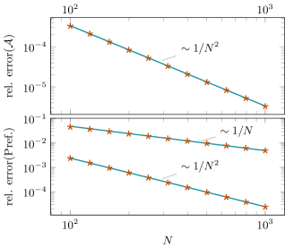
Figure 1: Accuracy of the method for a constant, homogeneous field. The error of the prefactor decreases as $1/N$ (the first order discretization error) for scalar QED (upper markers in the bottom plot), the error of the action as $1/N^{2}$ (because the action has an extremum at that point, upper plot). Interestingly, for spinor QED the prefactor decreases as $1/N^{2}$ as well (lower markers).

V Numerical continuation

For most fields we are interested in, there is one (or multiple) parameters that we would like to vary, for example the timescale of a pulsed field or the inhomogeneity of a spatially varying field configuration. Let us denote such a parameter $\gamma$. In general we are interested in the full family of instantons $\boldsymbol{\bar{X}}(\gamma)$. Methods to numerically map such a solution space are known as numerical continuation algorithms Allgower and Georg (2003); Rheinboldt (2000).

If we know an instanton for a particular value $\gamma_{i}$ of the parameter (e.g. the limit $\omega\to 0$ for a time-dependent pulse), we can use it as the starting point for the numerical solution of (24) for a parameter value $\gamma_{i+1}=\gamma_{i}+\Delta\gamma$, which is the method used in Gould and Rajantie (2017). If we choose a sufficiently small $\Delta\gamma$, we can expect the root finding procedure to quickly converge. This process is called natural parameter continuation, because we vary a physical parameter of the problem at hand, instead of introducing an artificial variable to blend between an easy and our actual problem (e.g. solving $0=\boldsymbol{G}(\boldsymbol{X},\gamma)\mathrel{\vbox{\hbox{\scriptsize.}\hbox{\scriptsize.}}}=\gamma\boldsymbol{F}(\boldsymbol{X})+(1-\gamma)\boldsymbol{F}_{0}(\boldsymbol{X})$).

Natural parameter continuation works well if the solutions $\boldsymbol{\bar{X}}(\gamma)$ depend on the parameter in a smooth and uniform manner. If, however, the dependence on $\gamma$ varies strongly, it is difficult to choose appropriate step lengths $\Delta\gamma$. For some spatially inhomogeneous fields the instantons even grow infinitely large in some limit $\gamma\to\gamma^{\text{crit}}$, so we need to take ever smaller steps to reach this value. We could, in principle, adaptively adjust the step length when the root finding for the next parameter value converges poorly, but there is an easier method of choosing the increment $\Delta\gamma$:

Natural parameter continuation can be viewed as a predictor-corrector scheme, with the “zeroth-order” predictor step of just taking the last solution as the starting point for the next parameter, and performing the numerical root finding as a corrector step. We can find a better prediction by taking the $\gamma$ derivative of (24), yielding the Davidenko differential equation Davidenko (1953):

$$\boldsymbol{0}=\frac{\mathrm{d}}{\mathrm{d}\gamma}\boldsymbol{F}(\boldsymbol{\bar{X}},\gamma)=\boldsymbol{\mathrm{H}}(\boldsymbol{\bar{X}},\gamma)\cdot\frac{\mathrm{d}\boldsymbol{\bar{X}}}{\mathrm{d}\gamma}+\frac{\partial}{\partial\gamma}\boldsymbol{F}(\boldsymbol{\bar{X}},\gamma)$$ (32)

and thus, provided that $\boldsymbol{\mathrm{H}}$ is invertible (which it is by our regularization scheme),

$$\frac{\mathrm{d}\boldsymbol{\bar{X}}}{\mathrm{d}\gamma}=-\left(\boldsymbol{\mathrm{H}}(\boldsymbol{\bar{X}},\gamma)\right)^{-1}\cdot\left(\frac{\partial}{\partial\gamma}\boldsymbol{F}(\boldsymbol{\bar{X}},\gamma)\right).$$ (33)

We can now use (33) in two ways: first, having found an instanton $\boldsymbol{\bar{X}}_{i}$ for a parameter value $\gamma_{i}$, it tells us in which way the instanton for a slightly different value of $\gamma$ differs from the current one, so we can use it as a much improved predictor in our predictor-corrector scheme, i.e. $\boldsymbol{\bar{X}}_{i+1}\approx\boldsymbol{\bar{X}}_{i}+\Delta\gamma\ \mathrm{d}\boldsymbol{\bar{X}}/\mathrm{d}\gamma$. In fact, we could directly integrate (33) to obtain all solutions. Unfortunately, evaluating the Hessian is costly and we can afford a much larger step size by performing the corrector steps. As a compromise it is possible to perform multiple steps according to (33) before starting the root finding routine. Furthermore, we can use the derivative to scale the step $\Delta\gamma$ by instead specifying a maximum (or mean) difference between the points of $\boldsymbol{\bar{X}}_{i}$ and the proposed guess for $\boldsymbol{\bar{X}}_{i+1}$, or even a fixed arclength $\Delta s$ of the solution curve in $\mathbb{R}^{N\times d+1}$,

$$\Delta s =\sqrt{(\Delta\gamma\ \mathrm{d}\boldsymbol{\bar{X}}/\mathrm{d}\gamma)^{2}+(\Delta\gamma)^{2}}$$

$$\Leftrightarrow\Delta\gamma =\frac{\Delta s}{\sqrt{(\mathrm{d}\boldsymbol{\bar{X}}/\mathrm{d}\gamma)^{2}+1}}.$$ (34)

A situation may be conceivable where it is not possible to parametrize the solution set as $\boldsymbol{\bar{X}}(\gamma)$ at all, because such a function would not be single-valued or have infinite slope somewhere. In this case, we can parametrize both the solution and the parameter $\gamma$ by a new parameter

$$\boldsymbol{\bar{Y}}(u) =(\boldsymbol{\bar{X}}(u),\gamma(u))^{\intercal}$$

$$\Rightarrow 0 =\frac{\mathrm{d}}{\mathrm{d}u}\boldsymbol{\tilde{F}}(\boldsymbol{\bar{Y}})=\boldsymbol{\mathrm{\tilde{H}}}\cdot\frac{\mathrm{d}\boldsymbol{\bar{Y}}}{\mathrm{d}u},$$ (35)

where $\boldsymbol{\mathrm{\tilde{H}}}$ is now an $(Nd+1)\times(Nd)$ matrix, so (35) has to be augmented by an additional condition. This is chosen to be a constraint on the orientation and the “velocity” of the flow $1=\left\lVert\mathrm{d}\boldsymbol{\bar{Y}}/\mathrm{d}u\right\rVert$, so $\boldsymbol{\bar{Y}}(u)$ is parametrized by arclength, hence the name pseudo-arclength continuation (pseudo because this is only approximately true, as we are taking discrete steps). As long as $\gamma$ is a suitable parameter, this is equivalent to (34), which is what we will be using in the following.

VI Applications

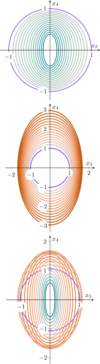
Figure 2: Planar instantons for multiple background fields and increasing values of $\gamma_{\omega/k}$. Top: temporal Sauter field $\boldsymbol{E}=E\cosh^{-2}(\omega t)\boldsymbol{e}_{z}$, middle: spatial Sauter field $\boldsymbol{E}=E\cosh^{-2}(kz)\boldsymbol{e}_{z}$, bottom: spacetime bump profile $\boldsymbol{E}=E\cosh^{-2}(\omega t)\cosh^{-2}(kz)\boldsymbol{e}_{z}$ with $k=3\omega$. The purple trajectories are the limit $\gamma_{\omega/k}\to 0$, blue denotes a decrease in action, red an increase. As is well known, while temporal variation shrinks the instantons and decreases the worldline action (top), spatial inhomogeneity has the opposite effect (middle). As the bottom plot shows, field configurations are possible that both increase and decrease the action in different regimes.

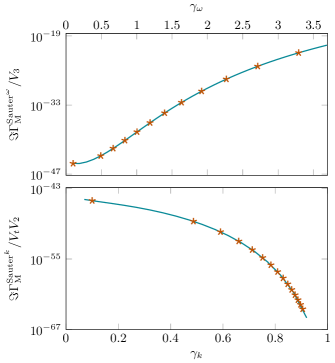
Figure 3: Imaginary part of the Minkowskian effective action (i.e. the pair production rate) for $E=0.033m^{2}/q$. Top: temporal Sauter pulse, bottom: spatial Sauter profile. Numerical results are given by markers and the analytic expressions (36) and (37) by lines. Note the spacing of markers in the spatial case, the step length decreases to keep the overall arclength $\Delta s$ constant.

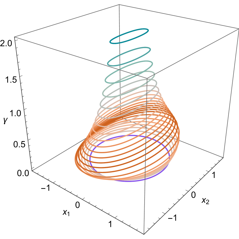
Figure 4: The same worldline instantons as in the third plot of Figure 2, but stacked, with the $z$-coordinate given by the parameter $\gamma$. This presentation makes it easier to correlate the instantons’ change in shape with the parameter.

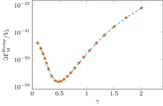
Figure 5: Imaginary part of the Minkowskian effective action for the spacetime bump profile $\boldsymbol{E}=E\cosh^{-2}(\omega t)\cosh^{-2}(kz)\boldsymbol{e}_{z}$ with $k=3\omega$ and $E=0.033m^{2}/q$. Here (and in the following cases) there are no analytical results to compare with, so we just add the connecting dashed lines as a guide to the eye.

Let us now apply the method outlined above to some background fields. The strategy in all cases is to start with a limit that is reasonably close to a static, homogeneous field and perform pseudo-arclength continuation to map the solution space for a chosen parameter range. In all figures depicting worldline instantons we color the homogeneous limit (i.e. a circular instanton) purple, and all further instantons proportional to the change in action (blue for a decrease, red for an increase, so blue means more, red less pair production). In all figures that show the full effective action we choose $E=0.033m^{2}/q$ for the reference field strength. This is simply the value we already used in earlier works, and it does not influence the quality of the discretization in any way. We also use $N=500$ points in the discretization, which yields good accuracy while it still takes less than thirty seconds to obtain the family of instantons in the cases below, with the exception of the $e$-dipole pulse.

VI.1 Temporal Sauter pulse

First let us consider simple, one-dimensional inhomogeneities where we can compare to analytic results. As an example, we choose the Euclidean four-potential $iA_{3}=\tan(\gamma_{\omega}x_{4})/\gamma_{\omega}$ describing the (physical) field $\boldsymbol{E}=E\cosh^{-2}(\omega t)\boldsymbol{e}_{z}$ with the Keldysh parameter $\gamma_{\omega}=m\omega/qE$ Keldysh (1965). Since the field does not depend on any spatial coordinates, we have $N_{0}=3$ translational zero modes that need to be held fixed.

The analytical worldline instanton result for this field is Dunne et al. (2006)

$$\frac{\Im\Gamma_{\mathrm{M}}^{\mathrm{Sauter}^{\omega}}}{V_{3}}=\frac{(qE)^{3/2}}{2(2\pi)^{3}}\frac{(1+\gamma_{\omega}^{2})^{5/4}}{\gamma_{\omega}}\\ \times\exp\left(-\frac{m^{2}\pi}{qE}\frac{2}{1+\sqrt{1+\gamma_{\omega}^{2}}}\right).$$ (36)

In Figure 2 the first plot shows a family of instantons in the range of $0<\gamma_{\omega}<3.5$, and the top panel in Figure 3 compares the numerical result (31) in this parameter range to the analytical expression (36), showing near-perfect agreement.

VI.2 Spatial Sauter pulse

We can also consider the spatially inhomogeneous profile $iA_{4}=\tanh(\gamma_{k}x_{3})/\gamma_{k}$ describing the (physical) field $\boldsymbol{E}=E\cosh^{-2}(kz)\boldsymbol{e}_{z}$ with (the spatial analog of) the Keldysh parameter $\gamma_{k}=mk/qE$. The analytical result is related to (36) by $\gamma_{\omega}\to i\gamma_{k}$ Dunne et al. (2006),

$$\frac{\Im\Gamma_{\mathrm{M}}^{\mathrm{Sauter}^{k}}}{V_{t}V_{2}}=\frac{(qE)^{3/2}}{2(2\pi)^{3}}\frac{(1-\gamma_{k}^{2})^{5/4}}{\gamma_{k}}\\ \times\exp\left(-\frac{m^{2}\pi}{qE}\frac{2}{1+\sqrt{1-\gamma_{k}^{2}}}\right),$$ (37)

where the instanton is now confined in $x_{3}$-direction and we obtain a “temporal volume factor” $V_{t}$ instead. The worldline instantons in this field for the range $0<\gamma_{k}<1$ are depicted in the middle of Figure 2, and the comparison of the numeric result and the analytic expression (37) in the bottom panel of Figure 3.

VI.3 Space-time Sauter pulse

As a simple example of a both space- and time-dependent background we choose the product of the preceding profiles with $\gamma:=\gamma_{\omega}=\gamma_{k}/3$, i.e. $iA_{3}=\cosh^{-2}(3\gamma x_{3})\tan(\gamma x_{4})/\gamma$. The resulting worldline instantons in the range $0<\gamma<2.5$ are shown in the bottom plot of Figure 2 and the resulting pair production rate in Figure 5. With the chosen ratio $\gamma_{k}/\gamma_{\omega}=3$ the spatial inhomogeneity dominates for small $\gamma$, giving larger instantons, increased action and lower pair production, while above $\gamma\approx 1$ the time dependence takes over and produces smaller instantons, reduced action and increased pair production.

VI.4 Multidimensional instantons

In Dunne and Wang (2006) multidimensional instantons were found for background fields that depend on multiple spatial coordinates using the shooting method. We can obtain instantons for these fields using discretization as well. Consider the potential

$$iA_{4}=\frac{1}{\sqrt{2}k}\frac{\tanh(kx_{1}+kx_{2})}{1+(kx_{1})^{2}+10(kx_{2})^{2}}$$ (38)

from Figure 1 in Dunne and Wang (2006) (with the factor of $1/\sqrt{2}$ added so the peak strength is $1$). This yields three dimensional instantons (in $x_{1}$-, $x_{2}$- and $x_{4}$-direction). Figure 6 depicts a family of instantons in a three dimensional plot, while Figure 8 shows all two dimensional projections of the same trajectories. The resulting pair production rate is given in Figure 7.

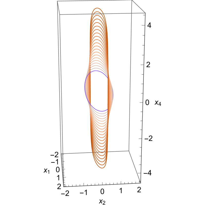
Figure 6: Worldline instantons for the four-potential (38) from Dunne and Wang (2006). As before, stronger inhomogeneity stretches the instantons (in a more complicated way than for the one dimensional fields) and increases the action.

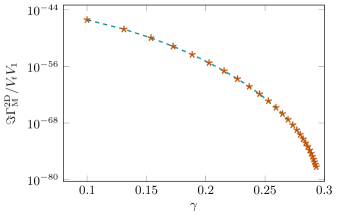
Figure 7: Imaginary part of the effective action for the multidimensional field from Dunne and Wang (2006) for $E=0.033m^{2}/q$. The dashed, connecting line is again a visual aid only.

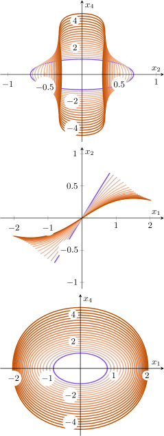
Figure 8: The same worldline instantons as in Figure 6, projected onto the coordinate planes.

VI.5 Plane wave plus electric field

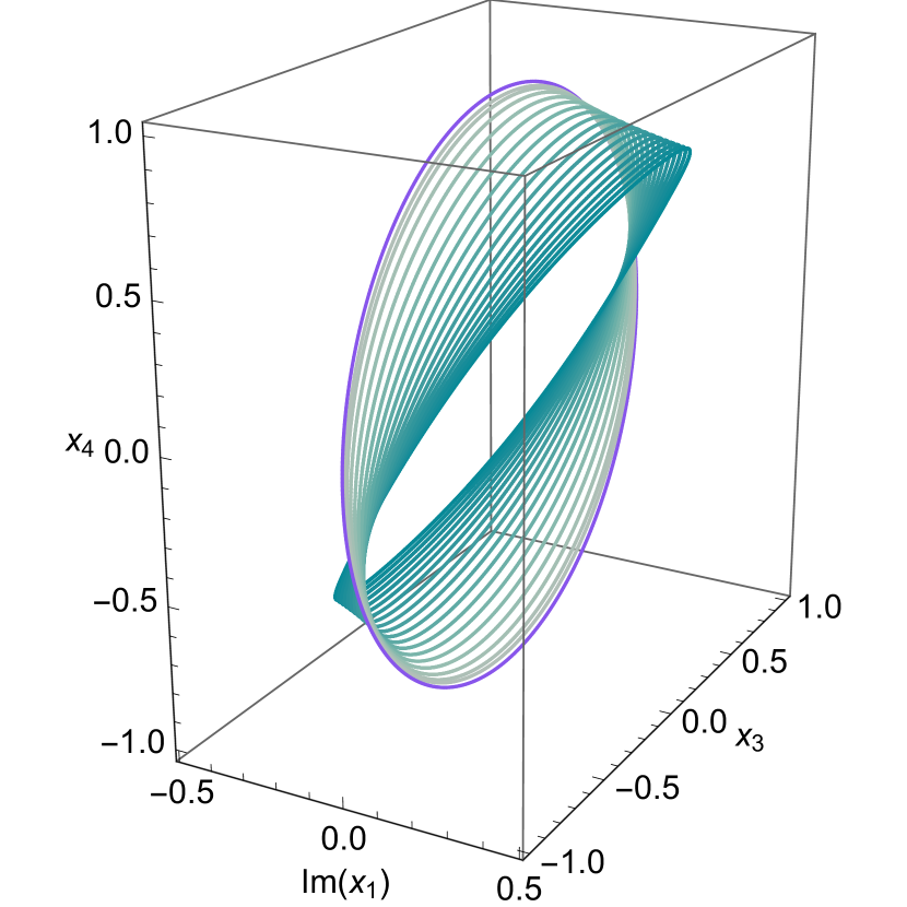
Figure 9: Worldline instantons for the superposition of a static, homogeneous field and a weak, propagating plane wave. The ratio of the plane wave amplitude and the strong field is $10^{-2}$. The $x_{1}$-component of the trajectories is purely imaginary, hence the imaginary part of $x_{1}$ on the first axis.

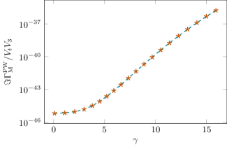
Figure 10: Pair production rate for a constant field ($E_{\mathrm{Strong}}=0.033m^{2}/q$) with superimposed plane wave ($E_{\mathrm{Weak}}=10^{-2}E_{\mathrm{Strong}}$). The temporal volume factor $V_{t}$ arises from the number of instantons, one per oscillation of the wave at a fixed spatial point. The dashed line is added as a guide to the eye.

Figure 11: The same worldline instantons as in Figure 9, projected onto the coordinate planes.

In Torgrimsson et al. (2018) we already applied the discrete worldline instanton method to calculate the pair creation rate for the superposition of a weak propagating plane wave and a constant field, a variant of dynamically assisted pair production Schützhold et al. (2008). Different pulse shapes have been considered for the weak field before Linder et al. (2015), however a plane wave is special in that it cannot produce pairs on its own, so the process is fully nonperturbative for all frequencies. In the case of parallel polarization (the plane wave and the constant field point in the same direction, but perpendicular to the propagation direction) this combination can be represented by the four-potential

$$iA_{4}=x_{3},\quad iA_{3}=i\frac{\varepsilon}{\gamma}\sin\left(\gamma(x_{1}-ix_{4})\right).$$ (39)

The method can handle the perpendicularly polarized case just as well, however that leads to four-dimensional instantons that are cumbersome to visualize.

In contrast to the examples considered before, the field (39) leads to complex instantons, in particular purely real $x_{3}(u)$, $x_{4}(u)$ and purely imaginary $x_{1}(u)$. A family of instantons is shown in Figures 9 and 11, while the full pair production rate is given in Figure 10.

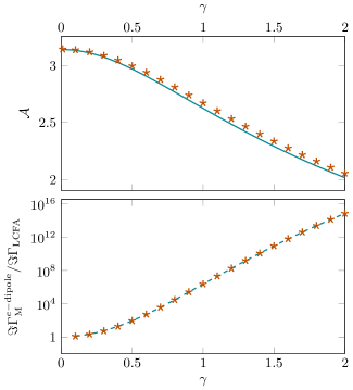
Figure 12: Top: Instanton action for the Gaussian e-dipole (40) (markers) compared to the action for a homogeneous field with Gaussian time dependence (line). Bottom: Ratio of the effective action and the locally constant field approximation for $E=0.033m^{2}/q$, with a dashed connecting line as a visual aid.

VI.6 E-dipole pulse

An especially interesting, highly non-trivial example is that of an e-dipole pulse. It is a solution to Maxwell’s equations in vacuum that represents a localized pulse of finite energy Gonoskov et al. (2012). It saturates the theoretical upper bound of peak field strength for given laser power Bassett (1986) and is thus in a sense the optimal (and at the same time physically viable) configuration to study pair creation Gonoskov et al. (2013). Its name stems from the structural similarity to dipole radiation, however it does not suffer from the strong singularities at the origin for a simple non-stationary dipole.

The electromagnetic field of the e-dipole pulse can be given in terms of a driving function $g$ using the vector $\boldsymbol{Z}$ Gonoskov et al. (2013)

$$\begin{split}\boldsymbol{Z}&=\boldsymbol{e}_{z}\frac{d}{\left|\boldsymbol{r}\right|}\Big{(}g(t+\left|\boldsymbol{r}\right|)-g(t-\left|\boldsymbol{r}\right|)\Big{)},\\ \boldsymbol{E}&=-\nabla\times\left(\nabla\times\boldsymbol{Z}\right),\quad\boldsymbol{B}=-\nabla\times\dot{\boldsymbol{Z}}.\end{split}$$ (40)

We choose the function

$$g(t)=\frac{t}{4\omega^{2}}e^{-\omega^{2}t^{2}}+\frac{\sqrt{\pi}}{8\omega^{3}}(1+2\omega^{2}t^{2})\operatorname{erf}(\omega t)$$ (41)

and the virtual dipole moment $d=3E/4$, so that at the origin

$$\boldsymbol{E}\approx Ee^{-\omega^{2}t^{2}}\boldsymbol{e}_{z}.$$ (42)

We cannot immediately apply the instanton approach to this field since it is not given in terms of a four-potential. It is however possible to obtain an expression for the potential in coordinate gauge $A(x)\cdot x=0$ from the field tensor Shifman (1980),

$$A^{\mathrm{M}}_{\mu}(x)=-\int\limits_{0}^{1}\!\mathrm{d}{\alpha}\ F^{\mathrm{M}}_{\mu\nu}(\alpha x)\,\alpha x^{\nu}.$$ (43)

For the field (40) this gives a lengthy expression, which can now be used to obtain worldline instantons.

Figure 12 shows the result. The top plot compares the instanton action for the e-dipole pulse to the action for a field with Gaussian time depencence only. Due to the additional spatial inhomogeneity in the e-dipole field the action is slightly larger (and thus pair production slightly lower) than for the purely time dependent pulse. We can also compare the full imaginary part of the effective action with the locally constant field approximation (in the bottom plot of Figure 12), which can be calculated using the saddle point method for $E$ below the critical field strength, giving

$$\Im\Gamma_{\mathrm{LCFA}}^{e\mathrm{-dipole}}\approx\frac{5\sqrt{5}}{2(2\pi)^{3}\gamma^{4}}\exp\left(-\pi\frac{m^{2}}{qE}\right).$$ (44)

As expected, the worldline instanton result tends to the locally constant field approximation for small values of $\gamma$, while it is exponentially larger for higher $\gamma$. For the parameters considered in Gonoskov et al. (2013) the adiabaticity is very small, with $\gamma<10^{-3}$, so the locally constant field approximation is accurate. For high frequency pulses however, the pair production rate is higher than the constant field estimate.

Figure 13: Top: Instanton action for a transversally polarized standing wave (markers) compared to just the oscillating time dependent field (line). Bottom: The same comparison for the imaginary part of the effective action with $E=0.033m^{2}/q$ including the prefactor. The transversal inhomogeneity does not change the exponent at all, but has a small effect on the prefactor.

VI.7 Transversal standing wave

Let us now briefly consider a purely transversal inhomogeneity. Two counterpropagating laser beams create a standing wave pattern, i.e. $\boldsymbol{E}=\cos(\omega t)\cos(kx)\boldsymbol{e}_{z}$ with $k=\omega$. In Lv et al. (2018) the authors find that omitting the spatial inhomogeneity leads to qualitatively incorrect results in the high frequency regime. In Aleksandrov et al. (2017) strong deviations in the momentum spectrum have been found in the homogeneous approximation as well.

In the semiclassical regime and for the total integrated rate however we can now check that approximating the standing wave by an oscillating homogeneous field works well. It is easy to see that the transversal inhomogeneity does not change the instanton and thus the action Linder et al. (2015), but the effect on the prefactor is not as obvious. Calculating the full effective action using the discrete instantons shows that while the prefactor does change, the difference from the homogeneous result is small and barely visible, see Figure 13. Note, however, that the momentum spectrum could still display noticeable differences between the standing wave and the purely time dependent field.

VI.8 Constant electric and magnetic fields

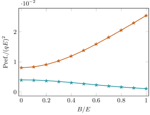
Figure 14: Prefactor divided by $(qE)^{2}$ for the sum of a constant electric field and a magnetic field with varying $B/E$. The markers show the discrete instanton result, the lines the analytic expressions (45). The results for scalar QED are blue, the results for spinor QED red.

In all examples up to now, the spin factor had only a small impact, apart from the trivial factor of two in the pair production probability. Let us finally consider a simple example where there is a large, qualitative difference between scalar and spinor QED, a parallel superposition of constant electric and magnetic fields of strength $E$ and $B$ respectively.

The (first term of) the effective action for this combination is given by (see e.g. Kim and Page (2006) and references therein)

$$\begin{split}\Gamma_{\mathrm{Scalar}}&\approx\frac{(qE)^{2}}{(2\pi)^{3}}\pi\frac{B}{E}\operatorname{csch}\left(\pi\frac{B}{E}\right)\exp\left(-\pi\frac{m^{2}}{qE}\right),\\ \Gamma_{\mathrm{Spinor}}&\approx\frac{2(qE)^{2}}{(2\pi)^{3}}\pi\frac{B}{E}\coth\left(\pi\frac{B}{E}\right)\exp\left(-\pi\frac{m^{2}}{qE}\right).\end{split}$$ (45)

Figure 14 depicts the prefactors of these expressions, so the $B/E$ dependence, together with the discrete instanton result, showing perfect agreement.

VII Summary and conclusion

We have introduced a new approach to numerically implement the worldline instanton method for electron-positron pair creation. We use a discretization scheme that turns the infinite-dimensional path integral into a finite dimensional integration that we can then perform using Laplace’s method. Crucially, this also means that the fluctuation prefactor is simply given by a finite dimensional determinant that can be computed without the great care that is needed for a properly normalized treatment of the functional determinant.

After having implemented the necessary root finding and continuation steps outlined in sections III, IV and V, full pair production results for arbitrary background fields can be obtained in minutes. Section VI gives a (by no means exhaustive) sample of such applications.

Although we used a frequency or inhomogeneity scale as the continuation parameter in all examples, we could have also chosen a different field parameter like the polarization direction or the ellipticity of the field, or even an entirely synthetic parameter to slowly transition to an especially complicated field configuration.

In this paper we have only considered cases for which there is one dominant instanton, which is continuously connected to a circular one in the constant field limit. It would be interesting for future studies to consider cases where there are more than one instanton, and where some of them might have a nontrivial topology.