On similarity flows for the compressible Euler system

Abstract.

Radial similarity flow offers a rare instance where concrete inviscid, multi-dimensional, compressible flows can be studied in detail. In particular, there are flows of this type that exhibit imploding shocks and cavities. In such flows the primary flow variables (density, velocity, pressure, temperature) become unbounded at time of collapse. In both cases the solution can be propagated beyond collapse by having an expanding shock wave reflect off the center of motion.

These types of flows are of relevance in bomb-making and inertial confinement fusion, and also as benchmarks for computational codes; they have been investigated extensively in the applied literature. However, despite their obvious theoretical interest as examples of unbounded solutions to the multi-dimensional Euler system, the existing literature does not address to what extent such solutions are bona fide weak solutions.

In this work we review the construction of globally defined radial similarity shock and cavity flows, and give a detailed description of their behavior following collapse. We then prove that similarity shock solutions provide genuine weak solutions, of unbounded amplitude, to the multi-dimensional Euler system. However, both types of similarity flows involve regions of vanishing pressure prior to collapse (due to vanishing temperature and vacuum, respectively) - raising the possibility that Euler flows may remain bounded in the absence of such regions.

1. Introduction

We consider two types of radial similarity flows for the compressible Euler system. These are particular types of solutions with planar (slab), cylindrical, or spherical symmetry. Under a similarity assumption the Euler system reduces to a coupled, nonlinear system of ODEs with respect to a similarity variable $x=t/r^{\lambda}$, where $t$ is time, $r$ is distance to the origin, and $\lambda$ is the similarity exponent. Similarity flows provide a rare instance where exact solutions to the multi-dimensional compressible Euler system can be constructed “by hand” and studied in considerable detail. Following Guderley’s pioneering study [gud], they have attracted substantial attention from physicists, engineers, and mathematicians. For a recent overview of the literature, see [rkb_12] and references therein.

The existing literature provides examples of similarity flows where a single (spherical or cylindrical) incoming shock wave propagates into a quiescent region about the origin (i.e., the fluid there is at rest and at constant density and pressure). The shock strengthens as it approaches the origin and the shock speed becomes unbounded at the instance of collapse at the origin. (For convenience, the time of collapse is chosen as $t=0$.) One can construct a complete (similarity) solution for all later times as well by having a diverging shock wave reflect off the origin. A different type of similarity solution describes the situation where a gas fills a spherical or cylindrical cavity (vacuum region) near the origin. Again, the speed of the fluid-vacuum interface blows up at collapse. Also in this case a global-in-time similarity solution can be constructed by inserting an outgoing shock after collapse. We refer to these two types of solutions as similarity shock and similarity cavity flows, respectively.

In either case the profiles for the fluid velocity, pressure, sound speed, and temperature at time of collapse are unbounded, with behavior given by negative powers of $r$ (in the cavity case, this applies also to the density profile). For this the similarity exponent must satisfy $\lambda>1$.

In Section 2 we record the multi-dimensional (multi-d) Euler equations for compressible flow of an ideal and polytropic gas with adiabatic exponent $\gamma>1$, including its radial form. We also posit the form of the radial similarity solutions under consideration. Section 3 outlines the setup for each type of solutions and collects various properties (initial data, jump relations, characteristics, etc.) of the similarity solutions under consideration.

For the actual construction of physically relevant similarity solutions with these properties, we follow Lazarus [L] who treats both shock and cavity flows. A complete breakdown of the various possibilities, including the key determination of allowed values of the similarity exponent $\lambda$, requires a detailed analysis and numerical calculations. Our main purpose of verifying that the Euler system admits unbounded weak solutions, does not require a full breakdown of all the cases. Instead, Section 4 outlines enough of this analysis to obtain some cases of Euler flows with unbounded amplitudes. In particular, we restrict attention to the standard value of the similarity exponent $\lambda$. This is the so-called “analytic” value, denoted $\lambda_{std}$ by Lazarus [L]. See Section 4 for details, where we also describe how the solutions are propagated past collapse to yield complete (i.e., global-in-time), radial similarity flows.

The resulting, well-known, solutions can be studied in detail. In particular, we deduce their asymptotic behavior at $x=+\infty$, which plays a key role in the analysis that follows. It turns out that the behavior of the resulting flows after collapse is markedly different near the center of motion in the shock case and in the cavity case; see Section 4.3. We also include a discussion to the effect that, at least among similarity flows, the continuation beyond collapse appears to be uniquely determined for both types of flows. Note that all jump discontinuities appearing in these similarity flows are, by construction, entropy admissible: both the incoming and the reflected shocks are compressive.

We then turn to our main concern: to what extent these types of similarity flows represent genuine weak solutions of the original, multi-d compressible Euler system. As the similarity solutions are singular and suffer blowup of primary flow variables at the origin, it is not immediately clear in what sense the weak form is satisfied. While some authors [bk, L] have addressed the constraint of locally finite energy for the similarity flows under consideration, we are not aware of a complete analysis. Concentrating on similarity shock solutions, we demonstrate that the flows constructed in the literature are indeed bona fide weak solutions whenever the similarity exponent $\lambda$ satisfies the constraint $\lambda\leq\frac{n}{2}+1$, where $n$ is $2$ or $3$ for cylindrical or spherical flow, respectively. The numerical values available in the literature indicate that the solutions corresponding to the particular value $\lambda_{std}$ always satisfy this constraint.

We shall show that the similarity shock solutions under consideration are bona fide weak solutions in the following sense: all terms occurring in the weak formulation of the multi-d Euler system are locally integrable in space-time; the amounts of mass, momentum, and energy within any fixed, compact spatial region change continuously with time (in particular, they are finite); and finally, the weak forms of the equations are satisfied. (Their total mass, momentum and energy in all of space are not bounded; however, this could be arranged via suitable modifications away from the origin without affecting the blowup behavior near the origin.)

We emphasize that we verify the weak form of the original, multi-d Euler system. Since the similarity solutions under consideration are radially symmetric, it is convenient to first derive the corresponding weak formulation for general radial solutions. This requires some care as the latter formulation involves different types of “test functions” for the different conservation laws. For completeness we include the derivation of the radial weak form of the equations (see Definition 2 and Proposition 5.1; here we follow the analysis [hoff] for radial Navier-Stokes flow).

With these preparations, Section 6 provides the details of the proof that genuine multi-d weak solutions are obtained from the radial symmetry solutions.

Discsussion

The existence of singular flows suffering point-wise blowup of flow variables is of obvious relevance in connection with the general Cauchy problem for the compressible Euler system. With the notable exception of small-variation data near a strictly hyperbolic state (Glimm [glimm]), there is currently no general, global-in-time existence result available for the one-dimensional (1-d) Cauchy problem for hyperbolic systems. (See [liu77, temple81] for extensions that cover certain types of large variation data specifically for the Euler system.) In more than one space dimension the situation is bleaker, and symmetric flows offer a natural case to consider in isolation. For results on isothermal and isentropic radial flow with general data, see [cp, cs, mmu].

In view of the blowup exhibited by similarity shock and similarity cavity solutions, it would appear that any existence result, applying to “general” data, for the multi-d Euler system would necessarily have to involve unbounded solutions. However, one should be careful not to draw too general conclusions on the basis of the similarity flows we study here. These are exceedingly special solutions, some aspects of which are borderline physical. In particular, both types of flows involve regions of vanishing pressure prior to collapse. In the case of a collapsing cavity this is due to the vacuum, and there is no reason why the Euler model should provide an accurate description close to its collapse. For the converging shock case, it turns out that the quiescent state into which the converging shock propagates, must necessarily be at zero pressure (due to vanishing temperature there) in order to generate an exact solution. In approximate treatments this amounts to a “strong shock” assumption.

For the case of an incoming shock, it is physically reasonable that a nonzero counter pressure would slow it down and possibly prevent unbounded amplitudes. This would provide a mechanism to “save” the Euler model from actual blowup. In particular, if indeed correct, this would show that the strong shock approximation fails to capture a crucial aspect of exact solutions near collapse of symmetric shock waves (blowup vs. no blowup of primary flow variables). We note that a number of works consider the effect of a positive counter pressure, e.g. [ah, phpm, welsh, vrt] and references therein. However, while amplitude blowup is still present in these works, none of them provide exact weak solutions to the Euler system.

The conventional point of view appears to be that the blowup exhibited by radial similarity flows results from multi-d wave focusing, much like what occurs for radial solutions to the linear 3-d wave equation. The remarks above raise the possibility that the unbounded amplitudes could be due to the presence of regions of vanishing pressure. We are not aware of a definite argument one way or the other - possibly both effects are required to generate blowup in $L^{\infty}$. Unfortunately, 1-d (slab symmetry) similarity flows do not help in assessing the situation: such solutions fail to generate physically acceptable flows; see Remark 4.1.

2. Equations

The full, multi-d Euler system for compressible gas flow is given by

(2.1) $$\rho_{t}+\operatorname{div}\left(\rho\vec{u}\right) =0$$

(2.2) $$\left(\rho\vec{u}\right)_{t}+\operatorname{div}\left(\rho\vec{u}\otimes\vec{u}\right)+\operatorname{grad}p =0$$

(2.3) $$\Big{[}\rho e+\frac{\rho|\vec{u}|^{2}}{2}\Big{]}_{t}+\operatorname{div}\Big{[}\Big{(}\rho e+\frac{\rho|\vec{u}|^{2}}{2}+p\Big{)}\vec{u}\Big{]} =0.$$

The variables are $\rho=$ density, $\vec{u}=$ fluid velocity, $p=$ pressure, $e=$ specific internal energy. Under the assumption of radial symmetry (i.e., all unknowns depend only on time $t$ and radial distance $r$ to the origin or an axis of symmetry, and $\vec{u}$ is purely radial), the system takes the form: ($u=|\vec{u}|$)

(2.4) $$\left(r^{m}\rho\right)_{t}+\left(r^{m}\rho u\right)_{r} =0$$

(2.5) $$\left(r^{m}\rho u\right)_{t}+\left(r^{m}(\rho u^{2}+p)\right)_{r} =mr^{m-1}p$$

(2.6) $$\Big{(}r^{m}\rho\Big{[}e+\frac{u^{2}}{2}\Big{]}\Big{)}_{t}+\Big{(}r^{m}\rho u\Big{[}e+\frac{u^{2}}{2}+\frac{p}{\rho}\Big{]}\Big{)}_{r} =0.$$

Here $r$ varies over $\mathbb{R}^{+}$, subscripts denote differentiation, and $m=1,\,2$ for flows with cylindrical or spherical symmetry, respectively. With $m=0$ and $r$ varying over $\mathbb{R}$, we have the one-dimensional Euler system. We consider an ideal, polytropic gas with equation of state

(2.7) $$p=(\gamma-1)\rho e=(\gamma-1)c_{v}\rho\theta,$$

where $\gamma>1$ and $c_{v}$ are positive constants, and $\theta=$ temperature. The specific entropy $S$ is related to $p$ and $\rho$ by

(2.8) $$p\rho^{-\gamma}=\text{Constant}\cdot\exp\Big{(}\frac{S}{c_{v}}\Big{)}.$$

It is a consequence of the conservation laws above that $S$ remains constant along particle trajectories in smooth regions of the flow:

(2.9) $$S_{t}+uS_{r}=0.$$

The sound speed $c$ is given by

(2.10) $$c^{2}:=\frac{\gamma p}{\rho}\equiv\gamma(\gamma-1)e,$$

and with $u$, $c$, and $\rho$ as primary unknowns, the system (2.4)-(2.6) takes the form:

(2.11) $$u_{t}+uu_{r}+\frac{1}{\gamma\rho}(\rho c^{2})_{r} =0$$

(2.12) $$c_{t}+uc_{r}+\frac{(\gamma-1)}{2}c\Big{(}u_{r}+\frac{mu}{r}\Big{)} =0$$

(2.13) $$\rho_{t}+u\rho_{r}+\rho\Big{(}u_{r}+\frac{mu}{r}\Big{)} =0.$$

Following the notation and setup of Lazarus [L], we introduce the similarity coordinate

(2.14) $$x=\frac{t}{r^{\lambda}},$$

where $\lambda$ is the similarity exponent (to be determined), and make the ansatz

(2.15) $$u(t,r) =-\frac{r}{\lambda t}\ V(x)=-\frac{r^{1-\lambda}}{\lambda}\frac{V(x)}{x}$$

(2.16) $$c(t,r) =-\frac{r}{\lambda t}\ C(x)=-\frac{r^{1-\lambda}}{\lambda}\frac{C(x)}{x}$$

(2.17) $$\rho(t,r) =r^{\kappa}R(x),$$

where $\kappa$ is a constant. We refer to solutions with this particular structure as similarity flows. Their relevance relies on the fact that they include physically meaningful flows where either symmetric shocks or cavities implode (converge, focus, collapse) at the origin. Similarity flows are determined via solutions to ODEs for $V$, $C$, and $R$. These are the similarity ODEs which we record in Section 3.3 below. We stress that, differently from many other cases of similarity solutions, the similarity exponent $\lambda$ is not given a priori, but must be determined as part of the solution.

3. Similarity shock and similarity cavity solutions

3.1. Similarity shock solutions

We shall first consider similarity flows where a single (spherical, cylindrical, or planar) shock moves toward the origin for negative times, and focuses at the origin at time $t=0$. Taking the existence of such similarity flows for granted for now, in this section we consider the Rankine-Hugoniot conditions, describe various constraints that should be met by physically relevant similarity flows, and describe a particular (critical) characteristic which plays a central role in the construction of such flows.

First, the flows on both sides of the shock are assumed to be similarity flows with the same values of $\lambda$, $\gamma$, and $\kappa$ in (2.15)-(2.17). We assume that the converging shock path is described by a constant value of the similarity variable $x$, say

(3.1) $$x\equiv-1\qquad\text{so that}\qquad r_{shock}=(-t)^{\frac{1}{\lambda}},\quad t<0.$$

We shall only consider situations where the shock reaches the origin with infinite speed, so that

(3.2) $$\lambda>1.$$

We follow [L] and let subscripts $0$ and $1$ denote evaluation immediately ahead of and behind of the shock, respectively. The (exact) jump relations and entropy condition then take the forms

(3.3) $$1+V_{1} =\frac{\gamma-1}{\gamma+1}(1+V_{0})+\frac{2C_{0}^{2}}{(\gamma+1)(1+V_{0})}$$

(3.4) $$C_{1}^{2} =C_{0}^{2}+\frac{\gamma-1}{2}[(1+V_{0})^{2}-(1+V_{1})^{2}]$$

(3.5) $$R_{1}(1+V_{1}) =R_{0}(1+V_{0})$$

(3.6) $$C_{0}^{2} <(1+V_{0})^{2}.$$

Here (3.6) expresses that the shock is supersonic relative to the state ahead; together these imply $C_{1}^{2}>(1+V_{1})^{2}$, amounting to the admissibility of the similarity shocks. The fluid on the inside (ahead) of the converging shock is assumed to be at rest and at constant density and pressure (quiescent state). According to (2.17), the constant density there dictates that $\kappa=0$ and $R(x)$ is constant; for concreteness let

$$R(x)\equiv 1\qquad\text{for $-\infty<x<-1$.}$$

Next, for an ideal gas $c^{2}\propto\frac{p}{\rho}$, so that the sound speed is constant in the quiescent region. As we assume $\lambda\neq 1$, (2.16) implies that $C$ must vanishes identically there. As the fluid near the origin is assumed to be at rest, we therefore have

$$V(x)=C(x)\equiv 0\qquad\text{for $-\infty<x<-1$.}$$

We are thus considering a single, converging shock which moves into a quiescent region at zero pressure and unit density. For an ideal polytropic gas, this means that the temperature vanishes identically in the region inside the converging shock.

With $(V_{0},C_{0},R_{0})=(0,0,1)$, inequality (3.6) is satisfied, and the jump relations (3.3)-(3.5) give the following initial conditions for the similarity variables $V$, $C$, $R$ at $x=-1^{+}$:

(3.7) $$V(-1)=V_{1}=-\frac{2}{\gamma+1},\qquad C(-1)=C_{1}=\frac{\sqrt{2\gamma(\gamma-1)}}{\gamma+1},\qquad R(-1)=R_{1}=\frac{\gamma+1}{\gamma-1}.$$

Along the immediate outside of the converging shock, the primary flow variables are therefore given by (2.15)-(2.17) as (recall that $\kappa=0$ in the present shock case):

(3.8) $$u=\frac{V_{1}}{\lambda}r^{1-\lambda}\qquad c=\frac{C_{1}}{\lambda}r^{1-\lambda}\qquad\rho\equiv R_{1}.$$

As we assume $\lambda>1$, it follows that the velocity $u$ and the sound speed $c$ become unbounded along the outside of the shock as it collapses at the origin, while the density remains finite. (The same applies along any curve given by $x\equiv constant\in(-1,0)$.)

Next, we are only interested in solutions where the flow variables $u$, $c$ and $\rho$ are “well behaved” at any location $r>0$ at time $t=0$. In particular, for any fixed $r>0$ we require that $u(t,r)$ and $c(t,r)$ tend to finite limits as $t\to 0$, i.e., as $x\to 0$. According to (2.15) and (2.16) we must therefore have that

(3.9) $$\ell:=\lim_{x\to 0}\frac{V(x)}{x}\qquad\text{and}\qquad L:=\lim_{x\to 0}\frac{C(x)}{x}\qquad\text{are finite,}$$

Thus, in particular, we have

(3.10) $$V(0)=C(0)=0.$$

It then follows from (2.15)-(2.16) and (3.9) that, at time of collapse ($t=0$), the radial flow speed $u$ and the sound speed $c$ blow up according to

(3.11) $$u(0,r)=-\frac{\ell}{\lambda}r^{1-\lambda}\qquad\text{and}\qquad c(0,r)=-\frac{L}{\lambda}r^{1-\lambda},$$

while the density is constant, $\rho(0,r)\equiv R(0)$. As a consequence, the pressure and temperature profiles at time of collapse blow up according to

(3.12) $$p(0,r),\,\theta(0,r)\,\propto\,r^{2(1-\lambda)}.$$

We point out that the limits in (3.9) will turn out to be non-zero and finite for the solutions constructed below. It follows that all three characteristic speeds ($u\pm c$ and $u$) are bounded at all points except at $(t,r)=(0,0)$. In particular, all fluid particles, except the one at the origin, are located away from $r=0$ at time $t=0$; in other words, the solutions under consideration are not of “cumulative” type where all (or a part of) the mass concentrates at the origin at collapse (examples of such flows are given in [kell, am]).

Next we note that, by (3.7),

(3.13) $$C>1+V>0\qquad\text{at $x=-1$},$$

while (3.10) shows that the opposite inequality holds at $x=0$. Thus, for some critical $x_{c}\in(-1,0)$ we must have

$$1+V(x_{c})=C(x_{c}).$$

(For the solutions considered below, there is a unique critical value $x_{c}$.) Now, to determine the full solution of the flow problem before collapse, we must integrate the similarity ODEs for $V(x)$, $C(x)$, and $R(x)$ for $x\in(-1,0)$, subject to the initial data in (3.7). It so happens that these ODEs are singular at points where $1+V=C$ (see (3.19)-(3.21)), and we have just seen that this must occur at some point $x_{c}\in(-1,0)$. The corresponding curve in the $(t,r)$-plane turns out to be a 1-characteristic for the corresponding Euler flow. (More generally, a calculation shows that the curve $x\equiv\bar{x}=constant$ is a 1-characteristic if and only if $1+V(\bar{x})=C(\bar{x})$.) Passing through $x=x_{c}$ corresponds to crossing the critical 1-characteristic, i.e. the 1-characteristic that catches up with the converging shock as it collapses at the origin. See Figure 1.

Figure 1. Converging similarity shock before collapse (schematic).

We point out that, in considering weak solutions, one should admit solutions with jumps in the derivatives of the flow variables across characteristics. In particular, $V$ and $C$ could enter and exit $x=x_{c}$ with different slopes. However, we shall not exploit this feature in the present work.

3.2. Similarity cavity solutions

For the case of a collapsing cavity we consider a spherical vacuum region centered at the origin, surrounded by fluid moving radially inward. Assuming for now the existence of similarity flows (2.15)-(2.17) with this structure, we assume that the vacuum-fluid interface follows the path $x=-1$ for negative times. Again we consider the case where this curve hits the origin with infinite speed at time $t=0$, so that $\lambda>1$. The interface is a particle trajectory, giving the initial condition for $V$ at $x=-1^{+}$ as

(3.14) $$V(-1)=-1.$$

To select initial conditions for $R$ and $C$ at $x=-1$, we impose the further constraint that the entropy takes a fixed, constant value $\bar{S}$ throughout the fluid region for negative times (before a shock is reflected off the origin). The fluid pressure is then given by $A\rho^{\gamma}$, where $A=A(\bar{S})$ is a constant. As the fluid pressure must vanish along the vacuum interface, it follows that the same holds for the density $\rho$, and also the sound speed $c=\sqrt{\gamma A\rho^{\gamma-1}}$. Equations (2.16) and (2.17) thus gives the initial conditions for $C$ and $R$ at $x=-1^{+}$ as

(3.15) $$C(-1)=R(-1)=0.$$

For later reference we note that isentropic similarity flow requires

(3.16) $$\kappa=-\frac{2(\lambda-1)}{\gamma-1};$$

this is a consequence of the momentum equation (2.11) with $\rho c^{2}=\gamma A\rho^{\gamma}$, upon substituting for $u$ and $\rho$ from (2.15) and (2.17), respectively.

It turns out that the similarity cavity flows constructed below immediately leaves the starting point $(V,C)=(-1,0)$ by moving into the region $C>1+V>0$. Just as for the shock case discussed above, we insist on “well-behaved” solutions satisfying (3.9). It follows that the cavity solution has to move back across the critical line $\{C=1+V\}$, for some $x_{c}\in(-1,0)$, before continuing on toward the origin.

We note that, in contrast to the case of a similarity shock, in similarity cavity flow only the fluid velocity $u$ blows up along the curve $x\equiv-1$, while $c$, $\rho$, $p$, and $\theta$ all vanish there. On the other hand, (2.15)-(2.17) imply that all of $u$, $c$, $\rho$, $p$, and $\theta$ blow up along all other curves $x\equiv constant\in(-1,0)$ as $t\uparrow 0$. (This last assertion requires that $V$ and $C$ does not vanish at any $x\in(-1,0)$; this will be the case for the similarity cavity flows constructed below.) Furthermore, the profiles for $u$, $c$, $p$, and $\theta$ at time of collapse are again given by (3.11)-(3.12) (provided the limits in (3.9) are non-zero, which holds for the cavity flows constructed below). Finally, for similarity cavity flow, also the density is unbounded at time $t=0$:

$$\rho(0,r)=R(0)r^{\kappa},$$

where $\kappa$, given by (3.16), is strictly negative since $\lambda>1$.

As the sound speed $c$ vanishes along the vacuum interface, the characteristics degenerate there and become tangent to the interface; a representative situation is recorded in Figure 2.

Remark 3.1.

It can be verified that the situation in Figure 2 is valid for the cavity flows constructed below. In particular, (4.1) yields $C\sim\sqrt{1+V}$ near $x=-1$, and this implies that any 1-characteristic between the interface $x=-1$ and the critical characteristic $x=x_{c}$ will meet the interface at a time strictly before collapse. It does so tangentially; at the same point a 3-characteristic starts off tangentially into the flow, as indicated.

Figure 2. Similarity cavity flow before collapse (schematic).

3.3. Similarity ODEs

Substituting (2.15)-(2.17) into (2.11)-(2.13) we obtain a system of three similarity ODEs for $V$, $C$, $R$. It is well-known that the constancy of specific entropy along particle trajectories provides one exact integral for the similarity ODEs (see [rj]). Specifically, in any region where the flow is smooth, we have

(3.17) $$R(x)^{q+1-\gamma}\left(\frac{C(x)}{x}\right)^{2}|1+V(x)|^{q}\equiv\text{constant},$$

where

(3.18) $$q=\frac{\kappa(\gamma-1)+2(\lambda-1)}{\kappa+n},$$

where $n=1,2,3$ is the spatial dimension. In the case of an incoming cavity, the flow is isentropic for $t<0$, and $q$ vanishes according to (3.16), while the right-hand side of (3.17) is determined once the constant value $\bar{S}$ of the entropy is assigned.

One can therefore obtain a closed system for two of the unknowns, the standard choice being $V$ and $C$. The resulting ODEs are (see [cf, L])

(3.19) $$V^{\prime}(x) =-\frac{1}{\lambda x}\frac{G(V(x),C(x),\lambda)}{D(V(x),C(x))}$$

(3.20) $$C^{\prime}(x) =-\frac{1}{\lambda x}\frac{F(V(x),C(x),\lambda)}{D(V(x),C(x))}$$

where ${}^{\prime}=\frac{d}{dx}$ and the polynomial functions $D$ and $G$, and the rational function $F$ are given by

(3.21) $$D(V,C) =(1+V)^{2}-C^{2}$$

(3.22) $$G(V,C,\lambda) =C^{2}\left[nV+{\textstyle\frac{2(\lambda-1)}{\gamma+s-1}}\right]-V(1+V)(\lambda+V)$$

(3.23) $$F(V,C,\lambda) =C\left\{C^{2}\left[1+{\textstyle\frac{s(\lambda-1)}{\gamma(1+V)}}\right]-\left[1+{\textstyle\frac{(n-1)(\gamma-1)}{2}}\right](1+V)^{2}\right.$$

$$\quad\qquad\left.+\left[{\textstyle\frac{(n-1)(\gamma-1)+(\gamma-3)(\lambda-1)}{2}}\right](1+V)-{\textstyle\frac{(\gamma-1)(\lambda-1)}{2}}\right\}.$$

Here $s$ is a logical variable: $s=1$ for the shock case and $s=0$ for the cavity case. Combining (3.19) and (3.20) we obtain a single ODE

(3.24) $$\frac{dC}{dV}=\frac{F(V,C,\lambda)}{G(V,C,\lambda)}$$

relating $V$ and $C$ along similarity solutions.

4. Construction of complete similarity flows

In this section we discuss the existence of solutions to the similarity ODEs, and how these are used to build physically meaningful similarity shock and similarity cavity flows. We seek complete solutions defined for all times.

The overall approach is, in principle, to solve (3.24) for $C=C(V)$ with the appropriate initial data, and substitute the result into (3.19)-(3.20) to obtain $x$-parametrizations for $V=V(x)$ and $C=C(x)$ via quadrature. From these $R=R(x)$ can be determined from the exact integral in (3.17). For the discontinuous solutions under consideration, the Rankine-Hugoniot relations (3.3)-(3.5) are used. These will uniquely determine the value of the constant on the right-hand side of (3.17) in each region where the solution is smooth. The original flow variables $\rho$, $u$, and $c$ are then given via (2.14)-(2.17). Finally one needs to verify that the solution so obtained is physically acceptable.

The analysis is complicated by the fact that the ODE (3.24) possesses a number of critical points (common zeros of $F$ and $G$), whose location varies with $\gamma$, $\lambda$, and $s$. Furthermore, these may or may not be located on the critical lines

$$\mathcal{C}_{\pm}:=\{C=\pm(1+V)\},$$

along which the denominator $D$ in (3.19) and (3.20) vanishes. As discussed below, this is a key issue. Among the many treatments in the literature we find the work [L] by Lazarus to be the most useful for our needs. (Lazarus also studies solutions with several converging similarity shocks, a scenario we do not consider in the present work.)

The location of the initial data for $(V,C)$ at $x=-1$ implies that the solutions of (3.24) need to cross the critical line $\mathcal{C}_{+}$, before continuing on to the origin in the $(V,C)$-plane. Let

$$\mathcal{F}:=\{(V,C)\,|\,F(V,C,\lambda)=0\},\qquad\mathcal{F}_{\pm}:=\mathcal{F}\cap\{C\gtrless 0\},$$

and define $\mathcal{G}$, $\mathcal{G}_{\pm}$ similarly by replacing $F(V,C,\lambda)$ by $G(V,C,\lambda)$. As shown in [L], the set $\mathcal{F}\cap\mathcal{G}$ of critical points for (3.24) can contain up to nine distinct points. One of these is $(V,C)=(-1,0)$, which is the initial point for similarity cavity flow. In addition there may be up to two more critical points located on $\mathcal{C}_{+}$; we follow Lazarus’ terminology and refer to these as points 6 and 8. Now, a similarity flow must solve the full ODE system (3.19) and (3.20). It follows from the form of these equations that any solution reaching the critical line $\mathcal{C}_{+}$, in order to continue on to the origin in the $(V,C)$-plane, must cross at a common zero of both $F$ and $G$. (Note that $F$ and $G$ are proportional along $\mathcal{C}_{\pm}$.) It is this restriction that is used to determine what the relevant values of $\lambda$ can be, for given values of $\gamma$, $n$, and $s$.

Lazarus [L] provides a detailed analysis of the subtle issue of which $\lambda$-values give complete flows. In particular, Lazarus defines a function $\lambda_{std}=\lambda_{std}(\gamma,n,s)$ by the property that the solution of (3.24), with $\lambda=\lambda_{std}$ and starting at the appropriate initial point, passes analytically through point 6 or point 8. As pointed out in [L], most other authors have considered $\lambda_{std}$ to be the only physically relevant value of the similarity exponent. Lazarus argues against this and shows that by removing the analyticity constraint one can, for fixed $\gamma$, $n$, and $s$, obtain whole families of complete similarity flows as $\lambda$ varies over certain non-trivial intervals. To obtain a complete breakdown of the possible cases requires numerical integration of the similarity ODEs. Most of the details of this analysis are included in [L]. In particular, the numerical values of $\lambda_{std}$ for $n=2,\,3$ and $s=0,\,1$ have been determined to several decimal places for a large number of $\gamma$-values (cf. Tables 6.2-6.5 in [L]). According to Lazarus, “Numerically, it has been determined beyond question that it [i.e., the function $\lambda_{std}$] exists for the shock problem for all $\gamma>1$, and for the cavity problem for $\gamma>\gamma_{std}$.” Here $\gamma_{std}$ depends on the spatial dimension and is approximately given by 2.9780 for $n=2$, and 2.4058 for $n=3$. In what follows we take these statements for granted. Differently from many other cases of similarity solutions to PDEs, the similarity exponent $\lambda$ is not apriori given; no analytic expression for $\lambda_{std}$ is known.

Having determined those $\lambda$-values which gives relevant solutions to the similarity ODEs (3.19) and (3.20) for $x\in(-1,0)$, it remains to continue the solution through the origin and extend it to all $x>0$. As commented earlier, this is accomplished by inserting an expanding similarity shock following a path of the form $r(t)=(\frac{t}{B})^{\frac{1}{\lambda}}$ for $t>0$ (i.e., $x\equiv B$, where $B>0$ is a constant). The determination of $B$ and the construction of the solution for $x\in(B,\infty)$ are outlined in Section 4.3 below; again, it appears necessary to do so through numerical integration of the equations.

Having constructed a complete similarity shock or cavity solution in this manner, it still remains to verify that the resulting flow is physically meaningful. This includes describing the solution behavior at the origin $r=0^{+}$ for $t>0$ (e.g., the velocity there should vanish), as well as checking that the mass, momentum, and total energy are locally bounded quantities. As we show in Section 6 (where we verify in detail that the similarity solutions are genuine weak solutions to the Euler system), the latter integral constraints require that the similarity exponent satisfies $\lambda<1+\frac{n}{2}$. It turns out that this is satisfied for all known values of $\lambda_{std}$ (cf. Tables 6.2-6.5 in [L]).

While we agree with [L] on the relevance of non-analytic similarity flows, the more important point, for our purposes, is that we obtain some examples of shock and cavity flows that exhibit blowup. We therefore restrict attention to solutions corresponding to the “analytic” similarity exponent $\lambda_{std}$.

4.1. Existence of similarity shock solutions prior to collapse

For the shock problem we first observe that, by construction, the converging shock along $x=-1$ is compressive. The same holds for the diverging shock following collapse. For the present case of an ideal gas, this implies that a fluid particle crossing the shock will suffer an increase in its physical entropy [gr_96]; i.e., all discontinuities under consideration involving jumps of primary (undifferentiated) flow variables, are genuine, “entropy-satisfying” shocks. Next, there is no issue near the initial point $(V_{1},C_{1})$ given by the two first expressions in (3.7): the ODE (3.24) is well behaved there and has a local solution for any values of $\lambda>1$ and $\gamma>1$. As outlined earlier, the solution must cross the critical line $\mathcal{C}_{+}=\{C=1+V\}$ before reaching $(V,C)=(0,0)$. As explained above we restrict attention to the particular value $\lambda=\lambda_{std}$ for which the solution crosses the critical line $\mathcal{C}_{+}$ in an analytic manner.

Remark 4.1.

The similarity ODEs (3.19)-(3.20) remain valid for $n=1$. However, an analysis reveals that the solution starting out from $(V_{1},C_{1})$ does not reach the critical line in this case, instead ending at a critical point $(\bar{V},\bar{C})$ lying strictly above $\mathcal{C}_{+}$ (this corresponds to “point 4” in Lazarus’ terminology [L]). The same applies to the case of 1-d similarity cavity flow. At $(\bar{V},\bar{C})$, $F(V,C)$ and $G(V,C)$ vanish and are Lipschitz continuous, while $D(V,C)$ does not vanish; therefore, the critical point is reached for $x=0$. However, (2.15) and (2.16) then imply that the resulting flow is physically meaningless at time of collapse in this case.

One could still attempt to build a 1-d flow exhibiting blowup by using only a part of the similarity flow just described, say the part corresponding to $x\in(-\infty,x_{0})$, for an $x_{0}<0$. The idea would be to complete the flow to all negative $x$, say, by a non-similarity flow (e.g., a simple wave). However, any change made in the original similarity flow for $x>x_{0}$ will necessarily influence the flow along the interface at $x=-1$, strictly before $t=0$, and thus possibly prevent blowup. This is a consequence of the fact that the original similarity solution does not reach the critical line $\mathcal{C}_{+}$: there is no critical 1-characteristic in this case (cf. Figure 2).

After crossing the critical line the $\lambda_{std}$-solution approaches the origin $(V,C)=(0,0)$, which is a star point for (3.24). $F(V,C)$ and $G(V,C)$ both vanish and are Lipschitz continuous at the origin, while $D(V,C)$ does not vanish there. It follows that the solution $(V(x),C(x))$ reaches the origin at $x=0$. This critical point is again crossed in an analytic manner and the solution continues into the lower half of the $(V,C)$-plane; see Section 4.3.

Remark 4.2.

According to (3.9) the solution $(V(x),C(x))$ approaches the origin with a slope $L/\ell$. For all cases we are aware of it is evident from numerical integration of the equations that the limits in (3.9) are non-zero and finite. It follows from (3.11) that the flow in these cases is “well-behaved” and physically meaningful at time of collapse.

4.2. Existence of cavity similarity solutions prior to collapse

For the cavity problem the initial point $(V,C)=(-1,0)$ for the ODE (3.24) lies on the critical line $\mathcal{C}_{+}=\{C=1+V\}$. This is a saddle point; a linearization about it in the variables $(V,Z=C^{2})$ shows that there is a solution leaving along the direction

(4.1) $$\frac{dZ}{dV}=\frac{\gamma(\gamma-1)(\lambda-1)}{n(\gamma-1)-2(\lambda-1)}.$$

The solution $C(V)$ to (3.24) therefore enters immediately the region $\{C>1+V>0\}$, provided $\lambda<1+\frac{n}{2}(\gamma-1)$, which we assume in what follows (for $s=0$).

Remark 4.3.

The corresponding solution $(V(x),C(x))$ of (3.19)-(3.20) has $C(x)\to 0$ as $x\downarrow-1$. Note that (3.17) (with $q=0$) also gives $R(x)\to 0$ as $x\downarrow-1$. It follows that the density $\rho$ vanishes as the interface $\{x=-1\}$ is approached from within the fluid. Therefore, the constructed solution satisfies the physical boundary condition that $p\propto\rho^{\gamma-1}$ vanishes along the vacuum interface.

Further along the solution, the situation is similar to that for the shock case: the similarity exponent $\lambda$ must be chosen so that the solution of (3.24) crosses the critical line $\mathcal{C}_{+}$ at a common zero of $F$ and $G$, i.e., through one of the critical points labeled 6 or 8 in [L]. Differently form the shock case, this will not occur for all values of $\gamma>1$. As noted earlier, for the cavity case, there is a minimal $\gamma_{std}(n)$ below which no value of $\lambda$ yields a solution with the required behavior.

After crossing the critical line $\mathcal{C}_{+}$, the situation is as in the shock case. The solution proceeds toward the origin in the $(V,C)$-plane, and passes through it in an analytical manner for $x=0$.

4.3. Existence of similarity solutions beyond collapse; the reflected shock

The works [L, RL_78, bg_96, RichtL_75, hun_60] consider the continuation of similarity shock and cavity solutions beyond collapse, to complete flows defined for all times. We are not aware of a general result addressing the unique continuation of solutions to (2.1)-(2.3), symmetric or not, for unbounded initial data. On the other hand, it is reasonable to assume that no symmetry breaking occurs at time of collapse, and restrict attention to radial similarity flows with the same values of $\lambda$ and $\kappa$ also for $t>0$. Furthermore, the unbounded pressure distribution at time of collapse (cf. (3.12)) suggests searching for a solution in which an expanding shock wave is generated at the origin at time zero.

Following [L, RL_78], we outline the construction of a reflected similarity shock propagating along a path $x=B=constant>0$. This shock will decay as it moves outward through the originally converging flow, leaving a non-isentropic flow region in its wake. Providing a complete solution requires the continuation of the similarity solution $(V(x),C(x))$ of (3.19)-(3.20) found earlier beyond $x=0$, the determination of the reflected shock path (i.e., the value of $B$), and the solution of (3.19)-(3.20) for all $x>B$. The latter part of the solution provides the flow in the wake of the reflected shock; in particular, the asymptotic behaviors of $V(x)$ and $C(x)$ as $x\uparrow\infty$ yield the behavior of the flow variables at the center of motion ($r=0$).

Continuing the solution $(V(x),C(x))$ through the star point (proper node) at the origin in the $(V,C)$-plane does not present any problem. This can be done in a unique analytic manner, and the solution $(V(x),C(x))$ is continued into the lower half-plane until it meets the critical line $\mathcal{C}_{-}=\{C=-1-V\}$. Following [L] we call this first part of the solution curve (in the lower half of the $(V,C)$-plane) “arc (a).”

For each point $(\tilde{V}_{0},\tilde{C}_{0})$ on arc (a), we then apply the Rankine-Hugoniot relations (3.3) and (3.4) to determine the unique point $(\tilde{V}_{1},\tilde{C}_{1})$, with $\tilde{C}_{1}<0$, to which the system can potentially jump. (Recall that the form (3.3)-(3.5) of the Rankine-Hugoniot relations assumes the discontinuity follows a “similarity path” $x=constant$, with the same values of $\lambda$, $\gamma$, and $\kappa$ on both sides of the discontinuity.) As was noted in connection with (3.3)-(3.5), since $\tilde{C}_{0}^{2}<(1+\tilde{V}_{0})^{2}$ along arc (a), the corresponding points $(\tilde{V}_{1},\tilde{C}_{1})$ necessarily lie below the critical line $\mathcal{C}_{-}$.

As $x$ increases from $0$, the point $(\tilde{V}_{0},\tilde{C}_{0})\equiv(V(x),C(x))$ moves away from the origin along arc (a). At the same time the corresponding point $(\tilde{V}_{1},\tilde{C}_{1})$ traces out a certain simple curve; we follow [L] and refer to it as the jump locus (of arc (a)). (This jump locus is the smiley, dotted curve in the lower half plane indicated in Figure 3 below.) According to (3.3)-(3.4) its left endpoint is $(V_{1},-C_{1})$ (corresponding to the point $(\tilde{V}_{0},\tilde{C}_{0})=(0,0)$), where $V_{1}$ and $C_{1}$ are given by (3.7). Its right end point lies on the critical line $\mathcal{C}_{-}$ and coincides with the end point of arc (a).

At this stage, each point on the jump locus (except its endpoints) provides possible initial data for (3.19)-(3.20), from which a solution trajectory should be continued for all $x>B$. The issue now is to argue that there is a unique point $(\hat{V}_{1},\hat{C}_{1})$ on the jump locus from which the solution can be continued to provide a physically meaningful solution to (2.1)-(2.3).

A computation shows that the ODE (3.24) has a critical point at $(V,C)=(V_{0},-\infty)$, where

(4.2) $$V_{0}=-\frac{2(\lambda-1)}{n(\gamma+s-1)}$$

gives the vertical asymptote for the zero-level of $G(V,C,\lambda)$ in the $(V,C)$-plane. This point corresponds to a saddle point at the origin in the variables $(v,\zeta)=(V-V_{0},C^{-2})$. There is therefore exactly one solution of (3.24) which approaches the vertical asymptote $V=V_{0}$. Furthermore, it appears that this solution, when integrated in from infinity, always lies entirely below the critical line $\mathcal{C}_{-}$, before intersecting the formerly determined jump locus at a single point $(\hat{V}_{1},\hat{C}_{1})$. This solution trajectory is referred to as “arc (b).” We then apply (3.3) and (3.4) to find the corresponding point $(\hat{V}_{0},\hat{C}_{0})$ on arc (a). The $x$-value $B$ at which the expanding shock is located is then determined by the condition that $(V(x),C(x))|_{x=B}=(\hat{V}_{0},\hat{C}_{0})$, where $(V(x),C(x))$ denotes the $x$-parametrization of arc (a). Modulo the $x$-parametrization of arc (b), this procedure determines the solution for all $x>0$, and provides a complete solution for both types of radial similarity flows.

Remark 4.4.

As is evident from Figure 8.30 in [L], and explicitly pointed out in [bg_96], for $\gamma\gtrsim 3$ and $n=3$, the similarity shock solution suffers stagnation ($u=0$) ahead of the reflected shock. In the phase plane this corresponds to the situation where the solution $(V(x),C(x))$ moves along arc (a) into the left half plane $\{V<0\}$ before jumping to arc (b).

Before addressing the uniqueness of this solution, we record how Lazarus [L] obtains the $x$-parametrization of arc (b). First $V$ and $C$ are expanded in powers of the new independent variable $w=kx^{-\sigma}$, where $k$ and $\sigma>0$ are constants to be determined. With the ansatz

(4.3) $$V(w)=\sum_{i=0}^{\infty}V_{i}w^{i}\qquad\text{and}\qquad C(w)=-\frac{1}{w}+\sum_{i=0}^{\infty}C_{i}w^{i},$$

substitution into (3.19) and (3.20) yields the value in (4.2) for $V_{0}$, and

(4.4) $$\sigma=\frac{1}{\lambda}\Big{[}1+\frac{s(n-1)z}{1+V_{0}}\Big{]}\qquad\text{where}\qquad z=\frac{\lambda-1}{(n-1)(\gamma+s-1)}.$$

To integrate the ODE system in from the critical point $(V_{0},-\infty)$ at infinity, Lazarus instead integrates the system for $V(w)$ and $C(w)$ from $w=0$, and thus obtains the $w$-parametrization of arc (b). This provides the value $w_{1}$ for which $(V(w),C(w))_{w=w_{1}}=(\hat{V}_{1},\hat{C}_{1})$, the point where arc (b) intersects the jump locus of arc (a). As explained above, this determines, via the Rankine-Hugoniot relations (3.3)-(3.4) and the $x$-parametrization of arc (a), the location $x=B$ of the reflected shock. Finally, the $x$-parametrization of arc (b) requires the determination of the constant $k$, which is now given by $k=B^{\sigma}w_{1}$.

Example 4.1.

In Figure 3 we have used Maple to display the complete similarity shock solution ($s=1$) in the $(V,C)$-plane for the case $n=\gamma=3$. We have used the values $\lambda=\lambda_{std}(3,3,1)\approx 1.5713126233$ and $B\approx 0.693970$ given by Table 6.5 in [L] (see erratum in [L_errat]). The solution starts at the starred point above the critical line $\{C=1+V\}$, moves downward, crosses $\{C=1+V\}$ and the origin smoothly, and then crosses the critical line $\{C=-1-V\}$ by jumping, before continuing along arc (b) toward the critical point at $(V_{0},-\infty)$. Note that, in accordance with Remark 4.4, the first jump point, corresponding to the state ahead of the reflected shock, is close to $\{V=0\}$.

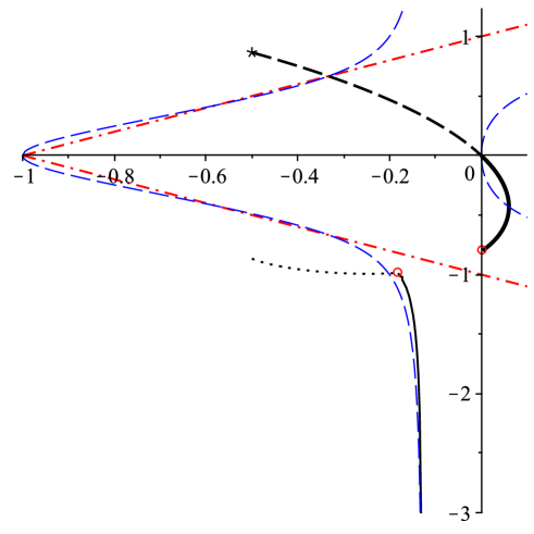
Figure 3. Complete trajectory of similarity shock solution ($n=\gamma=3$) in the $(V,C)$-plane. Thick dash $=$ solution for $-1<x<0$, thick solid $=$ arc (a), dotted $=$ jump locus, solid $=$ arc (b), thin dash $=$ zero-level of $G(V,C)$, dash-dot $=$ critical lines, star $=$ starting point, circles $=$ jump points.

We note that, according to (2.15), the physical requirement that the particle velocity $u(t,r)$ vanishes at the center of motion $r=0$ for all $t>0$, imposes the condition $V(x)/x^{\frac{1}{\lambda}}\to 0$ as $x\uparrow\infty$. Of course, this is satisfied for the solution determined above since $V(x)$ in that case tends to the finite limit $V_{0}$ as $x\uparrow\infty$.

By combining the asymptotic behavior of $V(x)$ and $C(x)$ with the exact integral (3.17) we obtain that of $R(x)$, and thus a complete description of the flow near the center of motion. A calculation shows that the result depends on the value of $s$; at any fixed time $t>0$ and as $r\downarrow 0$, we have:

• for similarity cavity flow ($s=0$): $\rho(t,r)$, $p(t,r)$, and $\theta(t,r)\propto c(t,r)^{2}$ all tend to nonzero constants (cf. Figures 8.19-8.22 in [L]);

• for similarity shock flow ($s=1$): $\rho(t,r)\to 0$, $p(t,r)$ tends to a strictly positive constant, while $c(t,r)$ and $\theta(t,r)$ both tend to $+\infty$ (cf. Figures 8.25-8.28 in [L]).

(For a representative calculation, see the proof of Lemma 6.1 below.) It is noteworthy that, in the case of similarity shock flow, the density vanishes at the center of motion after collapse, without the pressure tending to zero there. For the ideal gas under consideration, this yields unbounded temperature and sound speed at $r=0$ for $t>0$. (This contradicts Lazarus’ statement on p. 330 in [L] when $s=1$.) In our view, this is another manifestation of the borderline physicality of the radial similarity solutions under consideration.

It remains to discuss the uniqueness of the solution determined above, which was obtained by exploiting the critical (saddle) point $(V_{0},-\infty)$ at infinity for the ODE (3.24). Consider first similarity cavity flow ($s=0$), in which case (3.24) has critical points also at $(-\infty,-\infty)$ and at $(\infty,-\infty)$. However, neither of these appear to be reachable from the jump locus of arc (a). Indeed, from the phase portraits it appears that all solution trajectories $(V(x),C(x))$ starting from points on the jump locus lying to the left of $(\hat{V}_{1},\hat{C}_{1})$ end up (for a finite value of $x$) on the critical line $\mathcal{C}_{+}$, while all trajectories starting from points on the jump locus lying to the right of $(\hat{V}_{1},\hat{C}_{1})$ end up on $\mathcal{C}_{-}$. There is no way to continue these solutions to all $x>0$ and obtain complete, physically meaningful flows.

For the case of similarity shock flow ($s=1$), the ODE (3.24) has an additional critical point at $(V,C)=(-1,-\infty)$ (due to the $(1+V)^{-1}$-term in $F(V,C,\lambda)$ in this case, cf. (3.23)). From the phase portraits it appears that all solution trajectories $(V(x),C(x))$ starting from points on the jump locus lying to the left of $(\hat{V}_{1},\hat{C}_{1})$ approaches this point. (All trajectories starting from points on the jump locus lying to the right of $(\hat{V}_{1},\hat{C}_{1})$ appear again to end up on $\mathcal{C}_{-}$ for finite $x$-values). Changing to the variables $(V,\frac{1}{C})$ and linearizing, reveals that the point $(V,C)=(-1,-\infty)$ is necessarily reached for a finite $x$-value, say $\check{x}$ (depending on where along the jump locus the solution started). According to [RL_78], this shows that the critical point $(-1,-\infty)$ cannot describe the physical state at $r=0^{+}$ for $t>0$ (since this corresponds to $x=+\infty$), and is therefore irrelevant. However, this does not resolve the issue completely. A calculation shows that if $(V(x),C(x))$ of (3.19)-(3.20) tends to $(-1,-\infty)$ as $x\uparrow\check{x}$, then the density $\rho(t,r)$ at a fixed time $t>0$ will satisfy

$$\rho(t,r)\downarrow 0\quad\text{as}\quad r\downarrow\big{(}\textstyle\frac{t}{\check{x}}\big{)}^{\frac{1}{\lambda}};$$

that is, a vacuum is reached. This solution structure is not unreasonable: one might well imagine an expanding vacuum region opening up in the wake of a strong, expanding shock (a possibility considered by Hunter [hun_60] for the particular case of similarity cavity flow with $\gamma=7$). However, a further calculation reveals that the pressure $p(t,r)$ does not tend to zero as $r\downarrow(t/\check{x})^{1/\lambda}$ (for $t>0$ fixed). This type of solutions is therefore rejected as unphysical.

While these observations do not provide rigorous proof, they support the view that the only way to obtain a complete and physically admissible solution, is by having $(V(x),C(x))$ approach the saddle point at $(V_{0},-\infty)$ as $x\uparrow\infty$. It therefore appears that both similarity shock and similarity cavity solutions are uniquely determined beyond collapse - at least among similarity flows.

5. Weak and radial weak Euler solutions

We next consider whether the radial similarity solutions constructed above, considered as function of time and space, provide weak solutions to the original multi-d Euler system (2.1)-(2.3).

For concreteness, in what follows, we focus on the case of similarity shock solutions, in which case the radial velocity, sound speed, pressure and temperature are unbounded at time of collapse, cf. (3.11)-(3.12). The formulation and verification of the weak form of the equations therefore requires attention. Somewhat surprisingly this does not appear to have been addressed in the existing literature.

In this section we formulate the weak form of the Euler system (in the absence of vacuum regions), first for general, multi-d solutions, and then specialize it to the case of radial solutions.

5.1. General, multi-d weak solutions

We write $\rho(t)$ for $\rho(t,\cdot)$ etc., $\vec{u}=(u_{1},\dots,u_{n})$, $u:=|\vec{u}|$, and let $z=(z_{1},\dots,z_{n})$ denote the spatial variable in $\mathbb{R}^{n}$. We restrict attention to non-vacuum solutions.

Definition 1.

Consider the compressible Euler system (2.1)-(2.3) in $n$ space dimensions, with a given pressure function $p=p(\rho,e)\geq 0$, and let the measurable functions $\rho,\,u_{1},\dots,u_{n},\,e:\mathbb{R}_{t}\times\mathbb{R}_{z}^{n}\to\mathbb{R}$ be given. We say that these constitute a (non-vacuum) weak solution to (2.1)-(2.3) provided that:

• the functions $\rho$ and $e$ satisfy $\rho(t,z)>0$ and $e(t,z)\geq 0$ for a.a. $(t,z)\in\mathbb{R}\times\mathbb{R}^{n}$;

• the maps $t\mapsto\rho(t)$, $t\mapsto\rho(t)u(t)$, and $t\mapsto\rho(t)(e(t)+\frac{u(t)^{2}}{2})$ belong to $C(\mathbb{R}_{t};L^{1}_{loc}(\mathbb{R}^{n}_{z}))$;

• the functions $\rho u^{2}$, $p$, and $\big{[}\rho\big{(}e+\textstyle\frac{u^{2}}{2}\big{)}+p\big{]}u$ belong to $L^{1}_{loc}(\mathbb{R}_{t}\times\mathbb{R}^{n}_{z})$;

• the conservation laws for mass, momentum, and energy are satisfied weakly in sense that

  (5.1) $$\int_{\mathbb{R}}\int_{\mathbb{R}^{n}}\rho\varphi_{t}+\rho\vec{u}\cdot\nabla_{z}\varphi\,dzdt =0$$

  (5.2) $$\int_{\mathbb{R}}\int_{\mathbb{R}^{n}}\rho u_{i}\varphi_{t}+\rho u_{i}\vec{u}\cdot\nabla_{z}\varphi+p\varphi_{z_{i}}\,dzdt =0\qquad\text{for $i=1,\dots,n$}$$

  (5.3) $$\int_{\mathbb{R}}\int_{\mathbb{R}^{n}}\rho\big{(}e+\textstyle\frac{u^{2}}{2}\big{)}\varphi_{t}+\left[\rho\big{(}e+\textstyle\frac{u^{2}}{2}\big{)}+p\right]\vec{u}\cdot\nabla_{z}\varphi\,dzdt =0$$

  whenever $\varphi\in C_{c}^{1}(\mathbb{R}_{t}\times\mathbb{R}^{n}_{z})$ (the space of $C^{1}$-smooth functions with compact support).

Remark 5.1.

Note that we allow for the possibility that the density vanishes on sets of measure zero. This is relevant since, as noted above, the similarity shock solutions constructed earlier include a vacuum state at the center of motion after collapse.

Also, we do not address admissibility of weak solutions. While not the only possible approach, we consider the similarity shock solutions under consideration to be admissible since their discontinuities are, by construction, compressive shocks in ideal gases.

5.2. Radial weak Euler solutions

Next, for completeness we detail the relationship between weak solutions of the multi-d Euler system (2.1)-(2.3) and “radial weak solutions” of the radial version (2.4)-(2.6). This analysis has been provided earlier by Hoff [hoff] for radial solution of the compressible, isentropic Navier-Stokes system.

Setting $m:=n-1$ we let

$$\mathbb{R}^{+}=(0,\infty),\qquad\mathbb{R}_{0}^{+}=[0,\infty),\qquad L^{1}_{(loc)}(dt\times r^{m}dr)=L^{1}_{(loc)}(\mathbb{R}\times\mathbb{R}^{+}_{0},dt\times r^{m}dr),$$

and $C^{1}_{c}(\mathbb{R}\times\mathbb{R}^{+}_{0})$ denotes the set of real-valued functions $\psi(t,r)$ defined on $\mathbb{R}\times\mathbb{R}^{+}_{0}$ and with the property that $\psi$ is $C^{1}$ smooth on $\mathbb{R}\times\mathbb{R}^{+}_{0}$ and vanishes outside $[-\bar{t},\bar{t}]\times[0,\bar{r}]$ for some $\bar{t},\,\bar{r}\in\mathbb{R}^{+}$. In particular, for any $\psi$ in $C^{1}_{c}(\mathbb{R}\times\mathbb{R}^{+}_{0})$ the derivatives $\partial^{l}_{t}\partial_{r}^{k}\psi$ with $0\leq l+k\leq 1$ have well-defined (finite), continuous, and possibly non-vanishing, traces along the $t$-axis. Finally, we let $C^{1}_{0}(\mathbb{R}\times\mathbb{R}^{+}_{0})$ denote the set of functions $\psi\in C^{1}_{c}(\mathbb{R}\times\mathbb{R}^{+}_{0})$ with the additional property that $\psi(t,0)\equiv 0$.

Remark 5.2.

It follows from this that for any $\psi\in C^{1}_{0}(\mathbb{R}\times\mathbb{R}^{+}_{0})$, and any compact time interval $[-T,T]$, there is a constant $A=A_{\psi,T}$ so that

$$|\psi(t,r)|\leq Ar\quad\text{for all $t\in[-T,T]$.}$$

The relevance of these function classes is the following: when the weak formulation of the full multi-d Euler system (2.1)-(2.3) is applied to radial solutions, then the relevant “test functions” for the radial continuity and energy equations will belong to $C^{1}_{c}(\mathbb{R}\times\mathbb{R}^{+}_{0})$, while the relevant “test functions” for the radial momentum equation will belong to $C^{1}_{0}(\mathbb{R}\times\mathbb{R}^{+}_{0})$. Before verifying this we define “radial weak solutions.”

Definition 2.

Consider the radial version (2.4)-(2.6) of the compressible Euler system (2.1)-(2.3), where $(t,r)$ ranges over $\mathbb{R}\times\mathbb{R}^{+}$ and $p=p(\rho,e)\geq 0$ is a given pressure function.

Let the measurable functions $\rho,\,u,\,e:\mathbb{R}_{t}\times\mathbb{R}^{+}_{r}\to\mathbb{R}$ be given. We say that these constitute a (non-vacuum) radial weak solution to (2.4)-(2.6) provided that:

• the functions $\rho$ and $e$ satisfy $\rho(t,r)>0$ and $e(t,r)\geq 0$ for a.a. $(t,r)\in\mathbb{R}\times\mathbb{R}^{+}$;

• the maps $t\mapsto\rho(t)$, $t\mapsto\rho(t)u(t)$, and $t\mapsto\rho(t)(e(t)+\frac{u(t)^{2}}{2})$ belong to $C(\mathbb{R}_{t};L^{1}_{loc}(r^{m}dr))$;

• the functions $\rho u^{2}$, $p$, and $\big{[}\rho\big{(}e+\textstyle\frac{u^{2}}{2}\big{)}+p\big{]}u$ belong to $L^{1}_{loc}(dt\times r^{m}dr)$;

• the conservation laws for mass, momentum, and energy are satisfied in the distributional sense that

  (5.4) $$\int_{\mathbb{R}}\int_{\mathbb{R}^{+}}\left(\rho\psi_{t}+\rho u\psi_{r}\right)\,r^{m}drdt =0\qquad\forall\psi\in C^{1}_{c}(\mathbb{R}\times\mathbb{R}^{+}_{0})$$

  (5.5) $$\int_{\mathbb{R}}\int_{\mathbb{R}^{+}}\left(\rho u\psi_{t}+\rho u^{2}\psi_{r}+p\big{(}\psi_{r}+\textstyle\frac{m\psi}{r}\big{)}\right)\,r^{m}drdt =0\qquad\forall\psi\in C^{1}_{0}(\mathbb{R}\times\mathbb{R}^{+}_{0})$$

  (5.6) $$\int_{\mathbb{R}}\int_{\mathbb{R}^{+}}\left(\rho\big{(}e+\textstyle\frac{u^{2}}{2}\big{)}\psi_{t}+\left[\rho\big{(}e+\textstyle\frac{u^{2}}{2}\big{)}+p\right]u\psi_{r}\right)\,r^{m}drdt =0\qquad\forall\psi\in C^{1}_{c}(\mathbb{R}\times\mathbb{R}^{+}_{0}).$$

Proposition 5.1.

Consider the multi-d Euler system (2.1)-(2.3) with a given pressure function $p=p(\rho,e)$, together with its radially symmetric version (2.4)-(2.6). Then: given a radial weak solution $(\tilde{\rho},\tilde{u},\tilde{e})$ of (2.4)-(2.6), and setting

(5.7) $$\rho(t,z)=\tilde{\rho}(t,r)\qquad\vec{u}(t,z)=\tilde{u}(t,r)\frac{z}{r}\qquad e(t,z)=\tilde{e}(t,r)\qquad(r=|z|),$$

we obtain a weak solution $(\rho,\vec{u},e)$ of the multi-d Euler system (2.1)-(2.3).

Proof.

First, it is immediate that the properties in parts (i)-(iii) of Definition 2, together with (5.7), imply parts (i)-(iii) of Definition 1, respectively. It remains to verify the weak form of the equations. To verify (5.1) we fix $\varphi\in C_{c}^{1}(\mathbb{R}\times\mathbb{R}^{n})$ and set

(5.8) $$\psi(t,r):=\int_{|y|=1}\varphi(t,ry)\,dS_{y}.$$

Then $\psi\in C^{1}_{c}(\mathbb{R}\times\mathbb{R}^{+}_{0})$ and (5.4) gives

$$0 =\int_{\mathbb{R}}\int_{\mathbb{R}^{+}}\left(\tilde{\rho}\psi_{t}+\tilde{\rho}\tilde{u}\psi_{r}\right)\,r^{m}drdt$$

$$=\int_{\mathbb{R}}\int_{\mathbb{R}^{+}}\Big{[}\tilde{\rho}\int_{|y|=1}\varphi_{t}(t,ry)\,dS_{y}+\tilde{\rho}\tilde{u}\int_{|y|=1}\partial_{r}\left(\varphi(t,ry)\right)\,dS_{y}\Big{]}\,r^{m}drdt$$

$$=\int_{\mathbb{R}}\int_{\mathbb{R}^{+}}\int_{|y|=1}\Big{[}\tilde{\rho}\varphi_{t}(t,ry)+\tilde{\rho}\tilde{u}\nabla_{z}\varphi(t,ry)\cdot y\Big{]}\,r^{m}dS_{y}drdt=\int_{\mathbb{R}}\int_{\mathbb{R}^{n}}\rho\varphi_{t}+\rho\vec{u}\cdot\nabla_{z}\varphi\,dzdt,$$

verifying the weak form (5.1) of the continuity equation (2.1) in the multi-d Euler system.

Next, to verify (5.2) we fix $i$ ($1\leq i\leq n$) and $\varphi\in C_{c}^{1}(\mathbb{R}\times\mathbb{R}^{n})$, and set

(5.9) $$\psi(t,r):=\int_{|y|=1}y_{i}\varphi(t,ry)\,dS_{y}.$$

Then $\psi\in C^{1}_{0}(\mathbb{R}\times\mathbb{R}^{+}_{0})$ and (5.5) gives

(5.10) $$\int_{\mathbb{R}}\int_{\mathbb{R}^{+}}\Big{(}\underbrace{\tilde{\rho}\tilde{u}\psi_{t}}_{I}+\underbrace{\tilde{\rho}\tilde{u}^{2}\psi_{r}}_{I\!I}+\underbrace{\tilde{p}\big{(}\psi_{r}+{\textstyle\frac{m\psi}{r}}\big{)}}_{I\!I\!I}\Big{)}\,r^{m}drdt=0,$$

where $\tilde{p}=p(\tilde{\rho},\tilde{e})$. Treating each term in turn, we have:

$$I =\int_{\mathbb{R}}\int_{\mathbb{R}^{+}}\tilde{\rho}\tilde{u}\psi_{t}\,r^{m}drdt=\int_{\mathbb{R}}\int_{\mathbb{R}^{+}}\tilde{\rho}\tilde{u}\Big{[}\int_{|y|=1}y_{i}\varphi(t,ry)\,dS_{y}\Big{]}_{t}\,r^{m}drdt$$

$$=\int_{\mathbb{R}}\int_{\mathbb{R}^{+}}\int_{|y|=1}\tilde{\rho}\tilde{u}y_{i}\varphi_{t}(t,ry)\,r^{m}dS_{y}drdt=\int_{\mathbb{R}}\int_{\mathbb{R}^{n}}\rho u_{i}\varphi_{t}\,dzdt,$$

and

$$I\!I =\int_{\mathbb{R}}\int_{\mathbb{R}^{+}}\tilde{\rho}\tilde{u}^{2}\psi_{r}\,r^{m}drdt=\int_{\mathbb{R}}\int_{\mathbb{R}^{+}}\tilde{\rho}\tilde{u}^{2}\Big{[}\int_{|y|=1}y_{i}\varphi(t,ry)\,dS_{y}\Big{]}_{r}\,r^{m}drdt$$

$$=\int_{\mathbb{R}}\int_{\mathbb{R}^{+}}\int_{|y|=1}\tilde{\rho}\tilde{u}^{2}y_{i}\nabla_{z}\varphi(t,ry)\cdot y\,r^{m}dS_{y}drdt=\int_{\mathbb{R}}\int_{\mathbb{R}^{n}}\rho u_{i}\vec{u}\cdot\nabla_{z}\varphi\,dzdt.$$

For $I\!I\!I$ we first calculate

$$\left(r^{m}\psi\right)_{r} =\partial_{r}\Big{(}r^{m}\int_{|y|=1}y_{i}\varphi(t,ry)\,dS_{y}\Big{)}=\partial_{r}\Big{(}\int_{|z|=r}\varphi(t,z){\textstyle\frac{z_{i}}{|z|}}\,dS_{z}\Big{)}$$

$$=\partial_{r}\Big{(}\int_{|z|\leq r}\varphi_{z_{i}}(t,z)\,dz\Big{)}=\partial_{r}\Big{(}\int_{0}^{r}\int_{|y|=1}\varphi_{z_{i}}(t,sy)\,s^{m}dS_{y}ds\Big{)}=r^{m}\int_{|y|=1}\varphi_{z_{i}}(t,ry)\,dS_{y}.$$

Using this we obtain that

$$I\!I\!I =\int_{\mathbb{R}}\int_{\mathbb{R}^{+}}\tilde{p}\big{(}\psi_{r}+{\textstyle\frac{m\psi}{r}}\big{)}\,r^{m}drdt=\int_{\mathbb{R}}\int_{\mathbb{R}^{+}}\tilde{p}\left(r^{m}\psi\right)_{r}\,drdt$$

$$=\int_{\mathbb{R}}\int_{\mathbb{R}^{+}}\int_{|y|=1}\tilde{p}\varphi_{z_{i}}(t,ry)r^{m}\,dS_{y}drdt=\int_{\mathbb{R}}\int_{\mathbb{R}^{n}}p\varphi_{z_{i}}\,dzdt.$$

Substituting these expressions for $I$, $I\!I$, and $I\!I\!I$ back into (5.10), shows that the weak form (5.2) of the momentum equation (2.2) in the multi-d Euler system is satisfied.

Finally, to verify (5.3) we fix $\varphi\in C_{c}^{1}(\mathbb{R}\times\mathbb{R}^{n})$ and again define $\psi(t,r)$ by (5.8). Then $\psi\in C^{1}_{c}(\mathbb{R}\times\mathbb{R}^{+}_{0})$ and (5.6) gives

$$0 =\int_{\mathbb{R}}\int_{\mathbb{R}^{+}}\Big{(}\tilde{\rho}\big{(}\tilde{e}+{\textstyle\frac{\tilde{u}^{2}}{2}}\big{)}\psi_{t}+\Big{[}\tilde{\rho}\big{(}\tilde{e}+{\textstyle\frac{\tilde{u}^{2}}{2}}\big{)}+\tilde{p}\Big{]}\tilde{u}\psi_{r}\Big{)}\,r^{m}drdt$$

$$=\int_{\mathbb{R}}\int_{\mathbb{R}^{+}}\Big{\{}\tilde{\rho}\big{(}\tilde{e}+{\textstyle\frac{\tilde{u}^{2}}{2}}\big{)}\int_{|y|=1}\varphi_{t}(t,ry)\,dS_{y}$$

$$\qquad\qquad\qquad\qquad+\Big{[}\tilde{\rho}\big{(}\tilde{e}+{\textstyle\frac{\tilde{u}^{2}}{2}}\big{)}+\tilde{p}\Big{]}\tilde{u}\int_{|y|=1}\partial_{r}\left(\varphi(t,ry)\right)\,dS_{y}\Big{\}}\,r^{m}drdt$$

$$=\int_{\mathbb{R}}\int_{\mathbb{R}^{+}}\int_{|y|=1}\Big{\{}\tilde{\rho}\big{(}\tilde{e}+{\textstyle\frac{\tilde{u}^{2}}{2}}\big{)}\varphi_{t}(t,ry)$$

$$\qquad\qquad\qquad\qquad+\Big{[}\tilde{\rho}\big{(}\tilde{e}+{\textstyle\frac{\tilde{u}^{2}}{2}}\big{)}+p\Big{]}\tilde{u}y\cdot\nabla_{z}\varphi(t,ry)\Big{\}}\,r^{m}drdt$$

$$=\int_{\mathbb{R}}\int_{\mathbb{R}^{n}}\rho\big{(}e+{\textstyle\frac{u^{2}}{2}}\big{)}\varphi_{t}+\Big{[}\rho\big{(}e+{\textstyle\frac{u^{2}}{2}}\big{)}+p\Big{]}\vec{u}\cdot\nabla_{z}\varphi\,dzdt,$$

verifying the weak form (5.3) of the energy equation (2.3) in the multi-d Euler system. ∎

Remark 5.3.

Note that the “test function” $\psi$ in (5.8) typically has non-vanishing trace along the $t$-axis (e.g., when $n=3$, $\psi(t,r)\to 4\pi\cdot\varphi(t,0)$ as $r\downarrow 0$), while its $r$-gradient does vanish as $r\downarrow 0$. Also, the “test-function” $\psi$ in (5.9) behaves in the opposite manner: $\psi(t,r)\to 0$ as $r\downarrow 0$, while typically $\psi_{r}(t,r)\not\to 0$ as $r\downarrow 0$.

6. Similarity shock solutions as radial weak solutions

In this section we return to the case of an ideal gas and consider the similarity shock solutions constructed in Section 4 as candidates for weak solutions of the Euler system. The main result is that these provide bona fide weak solution that suffer blowup of primary flow variables at collapse. This conclusion holds for flows in two and three space dimensions provided the similarity shock solution $(R(x),V(x),C(x))$ satisfies the properties listed in (P1)-(P3) below. We stress that numerical computations clearly indicate that these properties are satisfied for the “standard” similarity solutions with $\lambda=\lambda_{std}(\gamma,n,1)$, for a large range of $\gamma$-values (see Tables 6.4-6.5 in [L]).

• the function $1+V(x)$ is uniformly bounded below away from zero, and from above, as $x$ varies over all of $\mathbb{R}$;

• the limits $\ell$ and $L$ in (3.9) satisfy $-\infty<L<0<\ell<\infty$;

• $(V(x),C(x))\to(V_{0},-\infty)$ as $x\uparrow\infty$, where $V_{0}$ is given by (4.2).

We now fix $n=2$ or $n=3$ and let $s=1$, such that $\kappa$ in (2.17) vanishes, and $\rho(t,r)=R(x)$.

Lemma 6.1.

With $n=2$ or $3$, and $1<\lambda<1+\frac{n}{2}$, assume (P1)-(P3) are satisfied for the solution $(R(x),V(x),C(x))$ under consideration. Then $R(x)>0$ for all $x\in\mathbb{R}$, the functions $R(x)$, $V(x)$, $V(x)/x$ are globally bounded on $\mathbb{R}$, and the functions $R(x)$, $V(x)/x$, $C(x)/x$ are continuous at $x=0$. Finally, the function $R(x)(C(x)/x)^{2}$ is globally bounded.

Proof.

Clearly, (P1) and (P2) imply global boundedness of $V(x)$, continuity of $V(x)/x$, $C(x)/x$ at $x=0$ (when the latter two functions are defined to take values $\ell$ and $L$ there, respectively), and therefore also global boundedness of $V(x)/x$.

Next, linearization of the ODE (3.24) about $(V_{0},-\infty)$ shows that the leading order behaviors of $V$ and $C$ there are given by (4.3)-(4.4):

(6.1) $$V(x)\sim V_{0}=-\frac{2(\lambda-1)}{\gamma n}\qquad\text{and}\qquad C(x)\sim-x^{\sigma}\qquad\text{as $x\uparrow\infty$},$$

where

(6.2) $$\sigma=\frac{1}{\lambda}\Big{(}1+\frac{\lambda-1}{\gamma-q}\Big{)}\qquad\text{with}\qquad q=\frac{2(\lambda-1)}{n}.$$

We note that the constraint $\lambda<1+\frac{n}{2}$ implies $-1<V_{0}<0$, and thus

(6.3) $$\gamma-q\equiv\gamma(1+V_{0})>0.$$

Also recall that the function $R(x)$ takes the value $1$ for $x<-1$; a calculation using the Rankine-Hugoniot relations (3.3)-(3.5) together with (3.17), shows that $R(x)>0$ for all $x>-1$ as well. By (3.17), the continuity of $V(x)$ and $C(x)/x$ at $x=0$ implies that of $R(x)$. According to (3.17) we also obtain

(6.4) $$R(x)\sim\big{(}\textstyle\frac{C(x)}{x}\big{)}^{-\frac{2}{q+1-\gamma}}\sim x^{-\frac{2}{\gamma-q}(1-\frac{1}{\lambda})}\qquad\text{as $x\uparrow\infty$.}$$

Thus, according to (6.3), we have that $R(x)$ tends to zero as $x\uparrow\infty$ (establishing the first part of (O2) in Section 4.3); it is therefore globally bounded. Finally, a similar calculation shows that

(6.5) $$R(x)\Big{|}\frac{C(x)}{x}\Big{|}^{2}\sim x^{-2(1-\frac{1}{\lambda})}.$$

Together with the continuity of $C(x)/x$ at $x=0$, this shows that $R(x)(C(x)/x)^{2}$ is globally bounded. ∎

For the solution $(R(x),V(x),C(x))$ under consideration we now define $\rho$, $u$, $c$, and $e$ via (2.15)-(2.17) and (2.10).

Theorem 6.2.

With $n=2$ or $3$, and under the assumption that (P1)-(P3) hold, the triple $(\rho,u,e)$ constitutes a radial weak solution to (2.4)-(2.6), with ideal pressure law (2.7), according to Definition 2 whenever

(6.6) $$1<\lambda<1+\textstyle\frac{n}{2}.$$

According to Proposition 5.1, it follows that these solutions provide (non-vacuum) weak solutions of the multi-d Euler system (2.1)-(2.3), according to Definition 1, with unbounded amplitudes.

The proof of Theorem 6.2 is organized as follows. First, part (i) of Definition 2 is immediate from Lemma 6.1 and the definitions of $\rho$ and $e$. The next two subsections consider the continuity and integrability requirements in parts (ii) and (iii) of Definition 2, respectively. Subsection 6.2.1 finishes the proof by analyzing the weak form of the equations (part (iv) of Definition 2).

6.1. Continuity and local integrability

For a fixed $\bar{r}>0$ and with

$$M(t;\bar{r}):=\int_{0}^{\bar{r}}\rho(t,r)r^{m}\,dr,\qquad I(t;\bar{r}):=\int_{0}^{\bar{r}}\rho(t,r)|u(t,r)|r^{m}\,dr,$$

$$E(t;\bar{r}):=\int_{0}^{\bar{r}}\rho(t,r)e(t,r)r^{m}\,dr+\frac{1}{2}\int_{0}^{\bar{r}}\rho(t,r)u^{2}(t,r)r^{m}\,dr=:E_{P}(t;\bar{r})+E_{K}(t;\bar{r}),$$

the issue is to show that the maps $t\mapsto M(t;\bar{r})$, $t\mapsto I(t;\bar{r})$, and $t\mapsto E(t;\bar{r})$ are continuous at all times $t\in\mathbb{R}$. Recall that the incoming and outgoing shock waves follow the paths $r=r_{i}(t)=(-t)^{1/\lambda}$ and $r=r_{o}(t)=(t/B)^{1/\lambda}$, respectively. In what follows we consider times $t$ small enough that $r_{i}(t)<\bar{r}$ if $t<0$ and $r_{o}(t)<\bar{r}$ if $t>0$. The calculations for the other cases are simpler and do not change the conclusions. We set

$$\alpha:=\frac{n}{\lambda}.$$

6.1.1. Continuity of $M(t;\bar{r})$

For $t<0$ we have $\rho(t,r)=1$ for $0<r<r_{i}(t)$, such that

(6.7) $$M(t;\bar{r})=\int_{0}^{r_{i}(t)}r^{m}\,dr+\int_{r_{i}(t)}^{\bar{r}}\rho(t,r)r^{m}\,dr=\frac{|t|^{\alpha}}{n}+\frac{1}{\lambda}|t|^{\alpha}\int_{-1}^{\frac{t}{\bar{r}^{\lambda}}}R(x)\,\frac{dx}{|x|^{\alpha+1}},$$

while for $t>0$ we have

(6.8) $$M(t;\bar{r})=\Big{[}\int_{0}^{r_{o}(t)}+\int_{r_{o}(t)}^{\bar{r}}\Big{]}\rho(t,r)r^{m}\,dr=\frac{1}{\lambda}t^{\alpha}\Big{[}\int_{\frac{t}{\bar{r}^{\lambda}}}^{B}+\int_{B}^{\infty}\Big{]}R(x)\,\frac{dx}{x^{\alpha+1}}.$$

As $R(x)$ is globally bounded, the integrals in (6.7) and (6.8) are all finite, and $t\mapsto M(t;\bar{r})$ is continuous at all times $t\neq 0$. For $t=0$ we have

(6.9) $$M(0;\bar{r})=\frac{\bar{r}^{n}}{n}R(0).$$

Observe that, as $R(x)$ is globally bounded, the second integral on the right-hand side of (6.8) and the first term on the right-hand side of (6.7) are of order $|t|^{\alpha}$, and thus vanish when $t\downarrow 0$ and $t\uparrow 0,$ respectively. Therefore, continuity from above at $t=0$ of $M(t;\bar{r})$ follows once it is established that

$$\frac{1}{\lambda}t^{\alpha}\int_{\frac{t}{\bar{r}^{\lambda}}}^{B}R(x)\,\frac{dx}{x^{\alpha+1}}\to M(0;\bar{r})\qquad\text{as $t\downarrow 0$.}$$

This may be verified by using L’Hôpital’s rule and the continuity of the map $x\mapsto R(x)$ at $x=0$. The same argument shows that

$$\frac{1}{\lambda}|t|^{\alpha}\int_{-1}^{\frac{t}{\bar{r}^{\lambda}}}R(x)\,\frac{dx}{|x|^{\alpha+1}}\to M(0;\bar{r})\qquad\text{as $t\uparrow 0$}$$

as well. Thus, the map $t\mapsto M(t;\bar{r})$ is continuous at all times.

6.1.2. Continuity of $I(t;\bar{r})$

For $t<0$ we have $u(t,r)=0$ for $0<r<r_{i}(t)$ such that

(6.10) $$I(t;\bar{r})=\int_{r_{i}(t)}^{\bar{r}}\rho(t,r)|u(t,r)|r^{m}\,dr=\frac{1}{\lambda^{2}}|t|^{\alpha-1+\frac{1}{\lambda}}\int_{-1}^{\frac{t}{\bar{r}^{\lambda}}}R(x)\frac{|V(x)|}{|x|}\,\frac{dx}{|x|^{\alpha+\frac{1}{\lambda}}},$$

while for $t>0$ we have

(6.11) $$I(t;\bar{r})=\Big{[}\int_{0}^{r_{o}(t)}+\int_{r_{o}(t)}^{\bar{r}}\Big{]}\rho(t,r)|u(t,r)|r^{m}\,dr=\frac{1}{\lambda^{2}}t^{\alpha-1+\frac{1}{\lambda}}\Big{[}\int_{\frac{t}{\bar{r}^{\lambda}}}^{B}+\int_{B}^{\infty}\Big{]}R(x)\frac{|V(x)|}{x}\,\frac{dx}{x^{\alpha+\frac{1}{\lambda}}}.$$

As $R(x)$ and $V(x)/x$ are globally bounded, and $\alpha+\frac{1}{\lambda}>1$ (by assumption (6.6)), the integrals in (6.10) and (6.11) are all finite, and $t\mapsto I(t;\bar{r})$ is continuous at any time $t\neq 0$. For $t=0$ we have, by property (P2) and with $\ell$ given by (3.9),

(6.12) $$I(0;\bar{r})=\frac{1}{\lambda}R(0)\ell\frac{\bar{r}^{n+1-\lambda}}{n+1-\lambda}.$$

As the second term on the right-hand side of (6.11) is of order $t^{\alpha-1+\frac{1}{\lambda}}$, and thus vanishes when $t\downarrow 0$ (by (6.6)), the continuity of $I(t;\bar{r})$ from above at $t=0$ follows once it is established that

$$\frac{1}{\lambda^{2}}t^{\alpha-1+\frac{1}{\lambda}}\int_{\frac{t}{\bar{r}^{\lambda}}}^{B}R(x)\frac{|V(x)|}{x}\,\frac{dx}{x^{\alpha+\frac{1}{\lambda}}}\to I(0;\bar{r})\qquad\text{as $t\downarrow 0$.}$$

This may be verified by using L’Hôpital’s rule and the continuity of the map $x\mapsto R(x)\frac{|V(x)|}{x}$ at $x=0$. The same argument shows that

$$\frac{1}{\lambda^{2}}|t|^{\alpha-1+\frac{1}{\lambda}}\int_{-1}^{\frac{t}{\bar{r}^{\lambda}}}R(x)\frac{|V(x)|}{|x|}\,\frac{dx}{|x|^{\alpha+\frac{1}{\lambda}}}\to I(0;\bar{r})\qquad\text{as $t\uparrow 0$}$$

as well. Thus, the map $t\mapsto I(t;\bar{r})$ is continuous at all times.

6.1.3. Continuity of $E(t;\bar{r})$

We consider first the kinetic energy

$$E_{K}(t;\bar{r})=\frac{1}{2}\int_{0}^{\bar{r}}\rho(t,r)u^{2}(t,r)r^{m}\,dr,$$

which is given for $t<0$ and $t>0$ by

(6.13) $$E_{K}(t;\bar{r})=\frac{|t|^{\alpha-2+\frac{2}{\lambda}}}{2\lambda^{3}}\int_{-1}^{\frac{t}{\bar{r}^{\lambda}}}R(x)\Big{|}\frac{V(x)}{x}\Big{|}^{2}\,\frac{dx}{|x|^{\alpha-1+\frac{2}{\lambda}}}$$

and

(6.14) $$E_{K}(t;\bar{r})=\frac{t^{\alpha-2+\frac{2}{\lambda}}}{2\lambda^{3}}\Big{[}\int_{\frac{t}{\bar{r}^{\lambda}}}^{B}+\int_{B}^{\infty}\Big{]}R(x)\Big{|}\frac{V(x)}{x}\Big{|}^{2}\,\frac{dx}{x^{\alpha-1+\frac{2}{\lambda}}},$$

respectively. Global boundedness of $R(x)$ and $V(x)/x$, together with assumption (6.6), imply that $t\mapsto E_{K}(t;\bar{r})$ is finite and continuous whenever $t\neq 0$. Evaluating at time $t=0$ yields, thanks to (6.6),

$$E_{K}(0;\bar{r})=\frac{1}{2\lambda^{2}}R(0)\ell^{2}\frac{\bar{r}^{n+2-2\lambda}}{n+2-2\lambda}.$$

As the second term on the right-hand side of (6.14) is of order $t^{\alpha-2+\frac{2}{\lambda}}$, and thus vanishes when $t\downarrow 0$ (by (6.6)), the continuity of $E_{K}(t;\bar{r})$ from above at $t=0$ follows once it is established that

$$\frac{t^{\alpha-2+\frac{2}{\lambda}}}{2\lambda^{3}}\int_{\frac{t}{\bar{r}^{\lambda}}}^{B}R(x)\left|\frac{V(x)}{x}\right|^{2}\,\frac{dx}{x^{\alpha-1+\frac{2}{\lambda}}}\to E_{K}(0;\bar{r})\qquad\text{as $t\downarrow 0$.}$$

Again, this follows by continuity of $R(x)|V(x)/x|^{2}$ at $x=0$ and L’Hôpital’s rule. The same argument applied to (6.13) shows that $E_{K}(t;\bar{r})$ tends to the same limit as $t\uparrow 0$. This shows that the map $t\mapsto E_{K}(t;\bar{r})$ is continuous at all times.

Finally, consider the potential energy:

$$E_{P}(t;\bar{r})=\int_{0}^{\bar{r}}\rho(t,r)e(t,r)r^{m}\,dr=\frac{1}{\gamma(\gamma-1)}\int_{0}^{\bar{r}}\rho(t,r)c^{2}(t,r)r^{m}\,dr,$$

which is given for $t<0$ and $t>0$ by

(6.15) $$E_{P}(t;\bar{r})=\frac{|t|^{\alpha-2+\frac{2}{\lambda}}}{\lambda^{3}\gamma(\gamma-1)}\int_{-1}^{\frac{t}{\bar{r}^{\lambda}}}R(x)\Big{|}\frac{C(x)}{x}\Big{|}^{2}\,\frac{dx}{|x|^{\alpha-1+\frac{2}{\lambda}}}$$

and

(6.16) $$E_{P}(t;\bar{r})=\frac{t^{\alpha-2+\frac{2}{\lambda}}}{\lambda^{3}\gamma(\gamma-1)}\Big{[}\int_{\frac{t}{\bar{r}^{\lambda}}}^{B}+\int_{B}^{\infty}\Big{]}R(x)\Big{|}\frac{C(x)}{x}\Big{|}^{2}\,\frac{dx}{x^{\alpha-1+\frac{2}{\lambda}}},$$

respectively. Global boundedness of $R(x)$ and $C(x)/x$, together with assumption (6.6), imply that $t\mapsto E_{P}(t;\bar{r})$ is finite and continuous at all times $t\neq 0$. Evaluating at time $t=0$ yields, thanks to (6.6),

$$E_{P}(0;\bar{r})=\frac{1}{\lambda^{2}\gamma(\gamma-1)}R(0)L^{2}\frac{\bar{r}^{n+2-2\lambda}}{n+2-2\lambda},$$

As the second term on the right-hand side of (6.16) is of order $t^{\alpha-2+\frac{2}{\lambda}}$(by (6.6)), the continuity of $E_{P}(t;\bar{r})$ from above at $t=0$ follows once it is established that

$$\frac{t^{\alpha-2+\frac{2}{\lambda}}}{\lambda^{3}\gamma(\gamma-1)}\int_{\frac{t}{\bar{r}^{\lambda}}}^{B}R(x)\left|\frac{C(x)}{x}\right|^{2}\,\frac{dx}{x^{\alpha-1+\frac{2}{\lambda}}}\to E_{P}(0;\bar{r})\qquad\text{as $t\downarrow 0$.}$$

As above this follows by L’Hôpital’s rule and the continuity of $R(x)|C(x)/x|^{2}$ at $x=0$. Finally, the continuity of $E_{P}(t,\bar{r})$ from below at time $t=0$ is established in the same manner.

This concludes the verification of part (ii) of Definition 2.

6.1.4. Local space-time integrability

Next, for part (iii) of Definition 2, we need to verify the local integrability in time and space of the functions $\rho u^{2}$, $p$, and $\big{[}\rho\big{(}e+\textstyle\frac{u^{2}}{2}\big{)}+p\big{]}u$. Recall that we consider an ideal gas (2.7), and that the incoming and outgoing shocks propagate along $x=-1$ and $x=B$, respectively. As a consequence, to verify part (iii) it suffices to show that, for any fixed $\bar{r}>0$, the space-time integrals

$$I_{\beta}(\bar{r}):=\int_{-\bar{r}^{\lambda}}^{B\bar{r}^{\lambda}}\int_{0}^{\bar{r}}\rho|u|^{\beta}r^{m}\,drdt,\qquad\text{for $\beta=2,\,3$,}$$

and

$$P_{\beta}(\bar{r}):=\int_{-\bar{r}^{\lambda}}^{B\bar{r}^{\lambda}}\int_{0}^{\bar{r}}p|u|^{\beta}r^{m}\,drdt,\qquad\text{for $\beta=0,\,1$,}$$

are finite. Transforming to $dxdt$-integrals, and recalling that the fluid is at rest on the inside of the incoming shock, we have

$$I_{\beta}(\bar{r}) =\frac{1}{\lambda^{\beta+1}}\left\{\int_{-1}^{B}\frac{R(x)|V(x)|^{\beta}}{|x|^{\alpha+1+\frac{\beta}{\lambda}}}\Big{[}\int_{0}^{|x|\bar{r}^{\lambda}}t^{\alpha+\beta\left(\frac{1}{\lambda}-1\right)}\,dt\Big{]}\,dx\right.$$

$$\qquad\qquad\qquad\left.+\Big{[}\int_{B}^{\infty}\frac{R(x)|V(x)|^{\beta}}{|x|^{\alpha+1+\frac{\beta}{\lambda}}}\,dx\Big{]}\Big{[}\int_{0}^{B\bar{r}^{\lambda}}t^{\alpha+\beta\left(\frac{1}{\lambda}-1\right)}\,dt\Big{]}\right\}$$

(6.17) $$=\frac{1}{\lambda^{\beta+1}}\frac{\bar{r}^{\lambda(\alpha+1)+\beta(1-\lambda)}}{(\alpha+1)+\beta\left(\frac{1}{\lambda}-1\right)}\left\{\int_{-1}^{B}\frac{R(x)|V(x)|^{\beta}}{|x|^{\beta}}\,dx+B^{\alpha+1+\beta\left(\frac{1}{\lambda}-1\right)}\int_{B}^{\infty}\frac{R(x)|V(x)|^{\beta}}{x^{\alpha+1+\frac{\beta}{\lambda}}}\,dx\right\}.$$

Here we have used that the $dt$-integrals are finite since, for all values of $\lambda$, $n$, and $\beta$ under consideration, (6.6) yields

$$\alpha+\beta\Big{(}\frac{1}{\lambda}-1\Big{)}>-1.$$

As $R(x)$, $V(x)/x$, and $V(x)$ are all globally bounded, it follows from (6.17) that $I_{\beta}(\bar{r})<\infty$ for any value of $\bar{r}$ and $\beta=2$ or $3$.

A similar computation for $P_{\beta}(\bar{r})$ (now using that the pressure $p$ vanishes on the inside of the incoming shock), yields

$$P_{\beta}(\bar{r}) =\frac{1}{\gamma\lambda^{\beta+3}}\left\{\int_{-1}^{B}R(x)\Big{|}\frac{C(x)}{x}\Big{|}^{2}\Big{|}\frac{V(x)}{x}\Big{|}^{\beta}\frac{1}{|x|^{\alpha+1+(2+\beta)(\frac{1}{\lambda}-1)}}\Big{[}\int_{0}^{|x|\bar{r}^{\lambda}}t^{\alpha+(2+\beta)\left(\frac{1}{\lambda}-1\right)}\,dt\Big{]}\,dx\right.$$

$$\qquad\qquad\qquad\left.+\Big{[}\int_{B}^{\infty}R(x)\Big{|}\frac{C(x)}{x}\Big{|}^{2}\Big{|}\frac{V(x)}{x}\Big{|}^{\beta}\frac{dx}{|x|^{\alpha+1+(2+\beta)(\frac{1}{\lambda}-1)}}\Big{]}\Big{[}\int_{0}^{B\bar{r}^{\lambda}}t^{\alpha+(2+\beta)\left(\frac{1}{\lambda}-1\right)}\,dt\Big{]}\right\}$$

$$=\frac{1}{\gamma\lambda^{\beta+3}}\frac{\bar{r}^{\lambda(\alpha+1)+(2+\beta)(1-\lambda)}}{(\alpha+1)+(2+\beta)\left(\frac{1}{\lambda}-1\right)}\left\{\int_{-1}^{B}R(x)\Big{|}\frac{C(x)}{x}\Big{|}^{2}\Big{|}\frac{V(x)}{x}\Big{|}^{\beta}\,dx\right.$$

(6.18) $$\qquad\qquad\qquad\left.+B^{\alpha+1+(2+\beta)\left(\frac{1}{\lambda}-1\right)}\int_{B}^{\infty}R(x)\Big{|}\frac{C(x)}{x}\Big{|}^{2}\Big{|}\frac{V(x)}{x}\Big{|}^{\beta}\frac{dx}{|x|^{\alpha+1+(2+\beta)(\frac{1}{\lambda}-1)}}\right\}.$$

Here we have used that the $dt$-integrals are finite since, for all values of $\lambda$, $n$, and $\beta$ under consideration, (6.6) yields

$$\alpha+(2+\beta)\left(\frac{1}{\lambda}-1\right)>-1.$$

By global boundedness of $R(x)$, $V(x)$, and $C(x)/x$, and by (6.6), both integrals on the right-hand side of (6.18) are finite for both $\beta=0$ and $\beta=1$.

This concludes the verification of part (iii) of Definition 2, under the constraint (6.6).

6.2. Weak form of the equations

Finally, for part (iv) of Definition 2, we need to verify the weak forms (5.4), (5.5), (5.6) of the radial equations. This requires some care since the solutions under consideration are unbounded at the origin. To handle this we shall exploit that the local integrability properties in parts (ii) and (iii) of Definition 2 have been verified under the condition (6.6). The issue then reduces to estimating the fluxes of the conserved quantities across spheres of vanishing radii.

6.2.1. Weak form of the mass equation

For a fixed $\psi\in C^{1}_{c}(\mathbb{R}\times\mathbb{R}^{+}_{0})$, with $\operatorname{supp}\psi\subset[-T,T]\times[0,A]$, and for any $\delta>0$, we have

$$M(\psi) :=\int_{\mathbb{R}}\int_{\mathbb{R}^{+}}\left(\rho\psi_{t}+\rho u\psi_{r}\right)\,r^{m}drdt=\left\{\int_{\mathbb{R}}\int_{0}^{\delta}+\iint_{I_{\delta}}+\iint_{I\!I_{\delta}}+\iint_{I\!I\!I_{\delta}}\right\}\left(\rho\psi_{t}+\rho u\psi_{r}\right)\,r^{m}drdt$$

(6.19) $$=:M_{\delta}(\psi)+\left\{\iint_{I_{\delta}}+\iint_{I\!I_{\delta}}+\iint_{I\!I\!I_{\delta}}\right\}\left(\rho\psi_{t}+\rho u\psi_{r}\right)\,r^{m}drdt$$

where the (open) regions $I_{\delta}$, $I\!I_{\delta}$, and $I\!I\!I_{\delta}$ are indicated in Figure 4 (e.g., $I_{\delta}$ is bounded below by $\{t=-T\}$, on the left by $\{r=\delta\}$, and on the right by the incoming shock path).

Figure 4. Regions of integration in the weak formulation.

Let ${\Gamma^{-}_{\delta}}$, ${\Gamma^{0}_{\delta}}$, and ${\Gamma^{+}_{\delta}}$ denote the parts of their boundaries $\partial I_{\delta}$, $\partial I\!I_{\delta}$, and $\partial I\!I\!I_{\delta}$, respectively, contained in the set $\{(t,r)\,|\,r=\delta\}$. Recall that the similarity shock solution is a bounded, classical solution of (2.4) in each of the regions $I_{\delta}$, $I\!I_{\delta}$, and $I\!I\!I_{\delta}$, and that the Rankine-Hugoniot conditions are satisfied across the incoming and outgoing shocks. Applying the divergence theorem therefore gives

$$M(\psi)=M_{\delta}(\psi)+\delta^{m}\left\{\int_{{\Gamma^{0}_{\delta}}}+\int_{{\Gamma^{+}_{\delta}}}\right\}(\rho u\psi)(t,\delta)\,dt,$$

where we have used that $u$ vanishes along ${\Gamma^{-}_{\delta}}$. By making the change of variables $t\mapsto x=t/\delta^{\lambda}$, we obtain

(6.20) $$M(\psi)=M_{\delta}(\psi)-\frac{\delta^{n}}{\lambda}\int_{-1}^{\frac{T}{\delta^{\lambda}}}R(x)\frac{V(x)}{x}\psi(x\delta^{\lambda},\delta)\,dx.$$

As $R(x)$, $V(x)/x$ are globally bounded, the last term in (6.20) is of order $\delta^{n-\lambda}$, which vanishes as $\delta\downarrow 0$ by (6.6). Finally, it follows from the analysis in Section 6.1 that both $\rho$ and $\rho u$ belong to $L^{1}_{loc}(r^{m}drdt)$. Thus, $M_{\delta}(\psi)\to 0$ as $\delta\downarrow 0$, so that $M(\psi)=0$ for each $\psi\in C^{1}_{c}(\mathbb{R}\times\mathbb{R}^{+}_{0})$. This shows that the weak form (5.4) of the radial mass equation is satisfied.

6.2.2. Weak form of the momentum equation

For a fixed $\psi\in C^{1}_{0}(\mathbb{R}\times\mathbb{R}^{+}_{0})$ and any $\delta>0$ we have

$$I(\psi) :=\int_{\mathbb{R}}\int_{\mathbb{R}^{+}}\left(\rho u\psi_{t}+\rho u^{2}\psi_{r}+p\big{(}\psi_{r}+\textstyle\frac{m\psi}{r}\big{)}\right)\,r^{m}drdt$$

$$=\left\{\int_{\mathbb{R}}\int_{0}^{\delta}+\iint_{I_{\delta}}+\iint_{I\!I_{\delta}}+\iint_{I\!I\!I_{\delta}}\right\}\left(\rho u\psi_{t}+\rho u^{2}\psi_{r}+p\big{(}\psi_{r}+\textstyle\frac{m\psi}{r}\big{)}\right)\,r^{m}drdt$$

(6.21) $$=:I_{\delta}(\psi)+\left\{\iint_{I_{\delta}}+\iint_{I\!I_{\delta}}+\iint_{I\!I\!I_{\delta}}\right\}\left(\rho u\psi_{t}+\rho u^{2}\psi_{r}+p\big{(}\psi_{r}+\textstyle\frac{m\psi}{r}\big{)}\right)\,r^{m}drdt.$$

Arguing as above and applying the divergence theorem gives ($x=t/\delta^{\lambda}$)

$$I(\psi) =I_{\delta}(\psi)+\delta^{m}\left\{\int_{{\Gamma^{0}_{\delta}}}+\int_{{\Gamma^{+}_{\delta}}}\right\}((\rho u^{2}+p)\psi)(t,\delta)\,dt$$

(6.22) $$=I_{\delta}(\psi)+\frac{\delta^{n+1-\lambda}}{\lambda^{2}}\int_{-1}^{\frac{T}{\delta^{\lambda}}}R(x)\Big{[}\Big{|}\frac{V(x)}{x}\Big{|}^{2}+\frac{1}{\gamma}\Big{|}\frac{C(x)}{x}\Big{|}^{2}\Big{]}\psi(x\delta^{\lambda},\delta)\,dx,$$

where we have used that $u$ and $p$ both vanish along ${\Gamma^{-}_{\delta}}$. Recalling the observation in Remark 5.2, and using global boundedness of $R(x)(V(x)/x)^{2}$ and $R(x)(C(x)/x)^{2}$, we obtain that

$$\delta^{n+1-\lambda}\int_{-1}^{\frac{T}{\delta^{\lambda}}}R(x)\Big{[}\Big{|}\frac{V(x)}{x}\Big{|}^{2}+\frac{1}{\gamma}\Big{|}\frac{C(x)}{x}\Big{|}^{2}\Big{]}\psi(x\delta^{\lambda},\delta)\,dx\lesssim\delta^{n+2-2\lambda},$$

which tends to zero as $\delta\downarrow 0$ by (6.6). Finally, to show that $I_{\delta}(\psi)$ also vanishes with $\delta$ we first use Remark 5.2 to bound the function $\frac{\psi}{r}$ by a constant, and then use that, according to the analysis above, the quantities $\rho u$, $\rho u^{2}$, and $p$ all belong to $L^{1}_{loc}(r^{m}drdt)$. This shows that also $I_{\delta}(\psi)\to 0$ as $\delta\downarrow 0$. Thus, $I(\psi)=0$ for each $\psi\in C^{1}_{0}(\mathbb{R}\times\mathbb{R}^{+}_{0})$, showing that the weak form (5.5) of the momentum equation is satisfied.

6.2.3. Weak form of the energy equation

For a fixed $\psi\in C^{1}_{c}(\mathbb{R}\times\mathbb{R}^{+}_{0})$ and any $\delta>0$ we have

$$E(\psi) :=\int_{\mathbb{R}}\int_{\mathbb{R}^{+}}\left(\rho\big{(}e+\textstyle\frac{u^{2}}{2}\big{)}\psi_{t}+\left[\rho\big{(}e+\textstyle\frac{u^{2}}{2}\big{)}+p\right]u\psi_{r}\right)\,r^{m}drdt$$

$$=\left\{\int_{\mathbb{R}}\int_{0}^{\delta}+\iint_{I_{\delta}}+\iint_{I\!I_{\delta}}+\iint_{I\!I\!I_{\delta}}\right\}\left(\rho\big{(}e+\textstyle\frac{u^{2}}{2}\big{)}\psi_{t}+\left[\rho\big{(}e+\textstyle\frac{u^{2}}{2}\big{)}+p\right]u\psi_{r}\right)\,r^{m}drdt$$

(6.23) $$=:E_{\delta}(\psi)+\left\{\iint_{I_{\delta}}+\iint_{I\!I_{\delta}}+\iint_{I\!I\!I_{\delta}}\right\}\left(\rho\big{(}e+\textstyle\frac{u^{2}}{2}\big{)}\psi_{t}+\left[\rho\big{(}e+\textstyle\frac{u^{2}}{2}\big{)}+p\right]u\psi_{r}\right)\,r^{m}drdt.$$

Arguing as above and applying the divergence theorem gives ($x=t/\delta^{\lambda}$)

$$E(\psi) =E_{\delta}(\psi)+\delta^{m}\left\{\int_{{\Gamma^{0}_{\delta}}}+\int_{{\Gamma^{+}_{\delta}}}\right\}\left[\rho u\big{(}e+\frac{1}{2}u^{2}+\frac{p}{\rho}\big{)}\psi\right](t,\delta)\,dt$$

(6.24) $$=E_{\delta}(\psi)+\frac{\delta^{n+2-2\lambda}}{\lambda^{3}}\int_{-1}^{\frac{T}{\delta^{\lambda}}}R(x)\frac{V(x)}{x}\left(\frac{1}{2}\left|\frac{V(x)}{x}\right|^{2}+\frac{1}{\gamma-1}\left|\frac{C(x)}{x}\right|^{2}\right)\psi(x\delta^{\lambda},\delta)\,dx,$$

where we have used that $u$ vanishes along ${\Gamma^{-}_{\delta}}$. Recalling the global boundedness of $R(x)$, $V(x)$, $V(x)/x$, and $R(x)(C(x)/x)^{2}$, as well as the bound (6.5), we obtain that the last integral in (6.24) is bounded by

$$\lesssim 1+\int_{1}^{\frac{T}{\delta^{\lambda}}}x^{-3}+x^{-2(1-\frac{1}{\lambda})-1}\,dx\lesssim 1+\delta^{2\lambda}+\delta^{2(\lambda-1)}\qquad\text{as $\delta\downarrow 0$.}$$

According to (6.6) we therefore have that the last term on the right-hand side of (6.24) vanishes as $\delta\downarrow 0$. Finally, under the same constraint on $\lambda$, the argument in Section 6.1 showed that the quantities $\rho e\propto p$, $\rho u^{2}$, $\rho ue\propto up$, and $\rho u^{3}$, all belong to $L^{1}_{loc}(r^{m}drdt)$. In particular, it follows that $E_{\delta}(\psi)$ vanishes as $\delta\downarrow 0$. Thus, $E(\psi)=0$ for each $\psi\in C^{1}_{c}(\mathbb{R}\times\mathbb{R}^{+}_{0})$, showing that the weak form (5.6) of the energy equation is satisfied.

This concludes the proof of Theorem 6.2.

Acknowledgment:

This work was supported in part by NSF awards DMS-1311353 (Jenssen) and DMS-1714912 (Tsikkou).