How Much Are You Willing to Share? A “Poker-Styled” Selective Privacy Preserving Framework for Recommender Systems

Abstract.

Most industrial recommender systems rely on the popular collaborative filtering (CF) technique for providing personalized recommendations to its users. However, the very nature of CF is adversarial to the idea of user privacy, because users need to share their preferences with others in order to be grouped with like-minded people and receive accurate recommendations. Prior related work have proposed to preserve user privacy in a CF framework through different means like (i) random data obfuscation using differential privacy techniques, (ii) relying on decentralized trusted peer networks, or (iii) by adopting secured cryptographic strategies. While these approaches have been successful inasmuch as they concealed user preference information to some extent from a centralized recommender system, they have also, nevertheless, incurred significant trade-offs in terms of privacy, scalability, and accuracy. They are also vulnerable to privacy breaches by malicious actors. In light of these observations, we propose a novel selective privacy preserving (SP2) paradigm that allows users to custom define the scope and extent of their individual privacies, by marking their personal ratings as either public (which can be shared) or private (which are never shared and stored only on the user device). Our SP2 framework works in two steps: (i) First, it builds an initial recommendation model based on the sum of all public ratings that have been shared by users and (ii) then, this public model is fine-tuned on each user’s device based on the user private ratings, thus eventually learning a more accurate model.

Furthermore, in this work, we introduce three different algorithms for implementing an end-to-end SP2 framework that can scale effectively from thousands to hundreds of millions of items. Our user survey shows that an overwhelming fraction of users are likely to rate much more items to improve the overall recommendations when they can control what ratings will be publicly shared with others. In addition, our experiments on two real-world dataset demonstrate that SP2 can indeed deliver better recommendations than other state-of-the-art methods, while preserving each individual user’s self-defined privacy.

1. Introduction

Collaborative filtering (CF) based recommender systems are ubiquitously used across a wide spectrum of online applications ranging from e-commerce (e.g. Amazon) to recreation (e.g. Spotify, Netflix, Hulu, etc.) for delivering a personalized user experience (Mishra and Reddy, 2016). CF techniques are broadly classified into two types – (i) classic Nearest Neighbor based algorithms (Takács et al., 2008) and more recent matrix factorization techniques (Koren et al., 2009), of which the latter has been more widely and predominantly adopted in industrial applications (Das et al., 2017) for building large-scale recommender models due to its superiority in terms of accuracy (Koren et al., 2009) and massive scalability (Oh et al., 2015; Karydi and Margaritis, 2016; Schelter et al., 2013; Meng et al., 2016; Xing, 2015; Li et al., 2016). Regardless of the underlying technique, the performance of a CF system is generally driven by the “homophilous diffusion” (Canny, 2002) process, where users must share some of their preferences in order to identify others with similar tastes and get good recommendations from them. The performance of CF algorithms often deteriorates without such adequate information, as often observed in the classic cold start (Volkovs et al., 2017) problem.

This inherent need for a user to share his/her preferences sometimes leads to serious privacy concerns. To make things more complicated, privacy is not a static concept and may greatly vary across different users, items and places. For example, different users under changing geopolitical, social and religious influences may have varying degree of reservation about explicitly sharing their ratings on sensitive items that deal with subjects like politics, religion, sexual orientation, alcoholism, substance abuse, adultery, etc. (Chow et al., 2012). Overall, these privacy concerns can prevent a user from explicitly rating many items, which reduces the overall performance of a CF algorithm, as compared to an ideal scenario, where everyone freely rates all the items they consume.

1.1. Motivation

In this paper, we explore the idea of letting each user define his/her own privacy. In other words, here the user decides which ratings he/she can comfortably share publicly with others, while his/her remaining ratings are considered as private, which means that they are stored only on the user’s device locally and are never shared with anyone including any peers or a centralized recommender system. Thus, this scheme enables each user to selectively define his/her own privacy. Figure 1 shows an example of such an operational setup.

Figure 1. Working of a selective privacy preserving (SP2) framework from a user’s perspective.

In this paper, we attempt to build a CF framework that preserves each user’s selective privacy and investigates the following issues in enabling such a framework:

$\bullet$ How can we build a selective privacy preserving (SP2) CF model that assimilates information from two kinds of ratings – all users’ public ratings and each user’s on-device private ratings?

$\bullet$ How can we ensure that there is no loss of private information in our SP2 framework?

$\bullet$ Can the SP2 framework improve the performance of a CF algorithm? In other words, does the SP2 framework improve the overall recommendation quality at all by taking into account each user’s private ratings? Or should the users simply hold back from rating sensitive materials if they have any privacy concern?

$\bullet$ Can this SP2 CF model ensure scalability with respect to industrial-scale datasets?

Interestingly, the selective privacy preserving framework proposed in this paper is somewhat analogous to the rules of a classic poker game (Omaha hold ‘em), where each player tries to form a best hand combining some of the community cards (which are publicly visible to everyone) and some of the hole cards (which are privately dealt to each player).

1.2. Contributions

In the rest of this paper, we address the questions listed in Section 1.1 and make the following contributions:

$\bullet$ We mathematically formulate the selective privacy preservation problem and present a formal framework to study it (Section 2). To the best of our knowledge, this is the first work under the umbrella of federated machine learning (Konećný et al., 2016) that supports a private on-device recommendation model for CF algorithms.

$\bullet$ We propose three different strategies (Section 3) for efficiently implementing an end-to-end SP2 framework, each of which is conducive to different situations. These underlying techniques overall ensure that a SP2 CF model incurs only a reasonable cost in terms of storage and communication overhead, even when dealing with massive industrial datasets or large machine learning models.

$\bullet$ We present analytical results on two real datasets comparing different privacy preserving and data obfuscation techniques to show the effectiveness of our SP2 framework (Section 4). We also empirically study what is a good information sharing strategy for any user in a SP2 framework and how much are the recommendations of a user affected, when he/she refrains from rating an item, instead of marking the latter as private.

$\bullet$ We present the results of a pilot study (Section 5), which demonstrates that an overwhelming majority of participants are willing to adopt this technology in order to receive more relevant recommendations without sacrificing their individual privacies.

2. SP2 Architecture

Our proposed selective privacy preserving (SP2) framework for CF algorithms is broadly based on the popular matrix factorization (MF) method, mainly due to its better performance, scalability and industrial applicability (Koren et al., 2009; Karydi and Margaritis, 2016; Schelter et al., 2013; Meng et al., 2016; Das et al., 2017). However, some of our discussions can also be extended to the traditional nearest neighbor based CF algorithms (Takács et al., 2008). We next briefly review the MF technique in Section 2.1.

2.1. Background

In the classic biased MF model (Koren et al., 2009), we try to learn the latent user and item factors (assumed to be in the same feature space of dimension $k$) from an incomplete ratings matrix (Takács et al., 2008). More formally, here, the estimated rating for a user $u$ on item $i$, $\hat{r_{ui}}$ is given by equation (1). The corresponding symbol definitions are provided in Table 1. We compute the user and item latent factors by minimizing the regularized squared error over all the known ratings, as shown in (2). This is done either using classic Alternating Least Squares method (Takács and Tikk, 2012; Das et al., 2017; Meng et al., 2016) which computes closed form solutions or via Stochastic Gradient Descent (SGD) (Koren et al., 2009), which enjoys strong convergence guarantees (Ge et al., 2016; Lee et al., 2016) and many desirable properties for scalability (Oh et al., 2015; Keuper and Pfreundt, 2015). The variable update equations for SGD are given by equation (3). For simplicity, we assume from now on that the user and item factors contain the respective biases i.e. user factor for $u$ ($p_{u}^{\prime}$) implies the column vector $[\,b_{u}\quad 1\quad p_{u}^{T}\,]^{T}$ and item factor for $i$ ($q_{i}^{\prime}$) refers to the column vector $[\,1\quad b_{i}\quad q_{i}^{T}\,]^{T}$.

(1) $$\hat{r_{ui}}=\mu+b_{u}+b_{i}+q_{i}^{T}p_{u}=\mu+q_{i}^{\prime T}p_{u}^{\prime}$$

Table 1. Definitions of symbols used in (1) - (3)

Symbol	Definition	Symbol	Definition
$\mu$	global mean of ratings	$\Omega$	set of observed ratings
$b_{u}$	bias for user $u$	$p_{u}$	latent vector for user $u$
$b_{i}$	bias for item $i$	$q_{i}$	latent vector for item $i$
$\delta$	Learning rate	$\lambda$	Regularization parameter
$r_{ui}$	actual rating of $i$ by $u$	$\hat{r_{ui}}$	prediction of $u$’s rating for $i$
$e_{ui}$	calculated as ($r_{ui}$-$\hat{r_{ui}}$)

(2) $$\text{min}\sum\limits_{r_{ui}\in\Omega}{(r_{ui}-\hat{r_{ui}})^{2}+\lambda(b_{i}^{2}+b_{u}^{2}+\parallel q_{i}\parallel^{2}_{2}+\parallel p_{u}\parallel^{2}_{2})}$$

(3) $$b_{u} \leftarrow b_{u}+\delta(e_{ui}-\lambda b_{u})$$

$$b_{i} \leftarrow b_{i}+\delta(e_{ui}-\lambda b_{i})$$

$$p_{u} \leftarrow p_{u}+\delta(e_{ui}q_{i}-\lambda p_{u})$$

$$q_{i} \leftarrow q_{i}+\delta(e_{ui}p_{u}-\lambda q_{i})$$

2.2. Problem Formulation

In a SP2 framework, each user $u$ has a set of public ratings, denoted by $\Omega^{u}_{\text{public}}$ and a set of private ratings, denoted by $\Omega^{u}_{\text{private}}$. However, since $\Omega^{u}_{\text{private}}$ is known only to $u$, the set of ratings observed here by the central recommender system is $\bigcup\limits_{u}\Omega^{u}_{\text{public}}$. We denote the latter by the notation $\Omega_{\text{public}}^{\prime}$. Now, our problem can be formulated as a multi-objective optimization problem, where we attempt to minimize $n$ regularized L2 loss functions together for $n$ users, as shown below:

min $(f_{1},f_{2},...,f_{n})$, where L2 loss ($f_{v}$) for user $v$ is given by,

$f_{v}:\big{[}\sum\limits_{r_{vj}\in\Omega^{v}_{\text{private}}}{(r_{vj}-\hat{r_{vj}})^{2}}\big{]}+\frac{1}{n}\sum\limits_{r_{ui}\in\Omega_{\text{public}}^{\prime}}{(r_{ui}-\hat{r_{ui}})^{2}}\\ \verb| |\qquad\qquad+\frac{\lambda}{n}(b_{i}^{2}+b_{u}^{2}+\parallel q_{i}\parallel^{2}_{2}+\parallel p_{u}\parallel^{2}_{2})\\$

Note, traditionally multi-objective optimization problems are solved with classic techniques like linear scalarization (also known as the weighted sum method (Grodzevich and Romanko, 2006)). In fact, if we assign equal weights to each user’s L2 loss function, then linear scalarization (Grodzevich and Romanko, 2006) can reduce this problem into a single-objective mathematical optimization problem (constructed as the weighted sum of the individual objective functions), which is similar to the one discussed in Section 2.1. However, due to privacy considerations, all of the data (users’ ratings) cannot be pooled together; this makes classic solutions to multi-objective optimizations problems inapplicable here. We next outline a privacy-aware model to solve this problem.

2.3. Model

We posit the following assumptions before summarizing our model.
Assumption 1. The central recommender system is semi-adversarial in nature i.e. it logs any information requested by a user and can later utilize it to guess what the user has rated privately.
Assumption 2. The central recommender system is not malicious in nature i.e. it will not deliberately send incorrect information to a user to adversely impact his/her recommendations. It has an incentive to provide high quality recommendations to the users.
Framework. Based on the earlier discussions, we now outline the working of our SP2 framework:

$(1)$ The central recommender system first builds a public model based on all the users’ shared public ratings using SGD. We obtain the public user and item factors when the error converges after a certain number of epochs.

$(2)$ Each user then downloads his/her corresponding public user factor from the central recommender system.

$(3)$ Additionally, all users’ also download common auxiliary public model data on their devices. This data is same for all users, and hence can be broadcasted by the central recommender system (for authentication in case the server cannot be trusted).

$(3)$ Once the auxiliary public model data and public user factor is locally available on the device, local updates are performed on the public user factor using auxiliary model information and the private ratings, which the user has saved on the device and has not shared with anyone.

$(4)$ The final private user factor and the private model are stored on the user’s device and never shared or communicated.

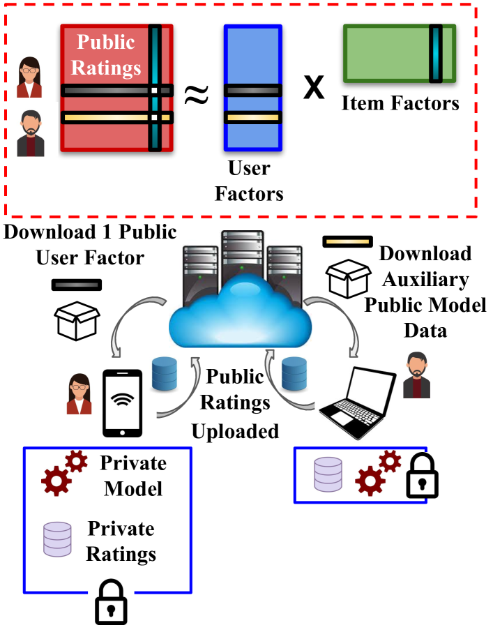
Figure 2. Architecture of a selective privacy preserving (SP2) framework.

Figure 2 presents the overall architecture. Interestingly, in our framework users never upload/communicate any private rating, even in encrypted format, thus guaranteeing privacy preservation. This is notably different from the general federated machine learning philosophy (Konećný et al., 2016; Bonawitz et al., 2017). We elaborate the need for this difference in Section 6.

Auxiliary public model data. It is also important to note that the central recommender system cannot share many parts of the public model with all the users. In many systems like Netflix, users only consent to rate a video on the condition that the central recommender system displays only the average rating for the video, instead of the individual ratings from the users’ community. In such cases, the auxiliary public model data cannot contain ratings from $\Omega_{\text{public}}^{\prime}$, as the latter scenario also constitutes a user-privacy breach, since the users may not be comfortable sharing their explicit ratings information with each other. In the same vein, consider the example, where the auxiliary public model data comprises of both public user factors and item factors. This information alone is sufficient to identify the corresponding public ratings for other users with reasonable confidence, thus again breaching user privacy. Furthermore, even anonymizing this information is not enough to prevent privacy leaks as demonstrated through de-anonymization attacks on Netflix dataset (Narayanan and Shmatikov, 2008). Thus, the auxiliary public model data needs to be designed carefully so that it not only facilitates in building a better private model on the user’s device, but also simultaneously safeguards the SP2 framework from privacy breaches. In light of this, observe that the auxiliary public model data can comprise of public item factors alone. Each public item factor is updated over a set of users based on their public user factors and ratings. Thus, only the set of final public item factors alone do not constitute a user-privacy breach.

Private ratings distribution. For analyzing the efficacy of our SP2 framework, it is also important to consider how users privately rate an item. We examine two different hypotheses for modeling this:

$\bullet$ Hypothesis 1 (H1). Users always decide independently which of his/her ratings are private. Formally, for any two users $x$ and $y$, who have rated an item $i$ with ratings $r_{xi}$ and $r_{yi}$ respectively, $P(r_{xi}$ is private $|$ $r_{yi}$ is private$)=P(r_{xi}$ is private$)$.

$\bullet$ Hypothesis 2 (H2). Users do not decide independently which of his/her ratings are private. In other words, ratings for some items are more likely to be marked as private. Formally, using the same mathematical notations as above, $P(r_{xi}$ is private $|$ $r_{yi}$ is private$)\neq P(r_{xi}$ is private$)$.

In Section 4, we further discuss how private ratings are allocated in our experiments based on these two hypotheses.

3. Implementation

In this section, we present three approaches for implementing our SP2 framework.

3.1. Naive Approach

In this approach, the auxiliary public model data contains the entire item factor matrix (i.e. all the latent item vectors and their biases). Each user’s on-device private model is then built following the steps shown in algorithm 1. The update equation used in this algorithm are similar to the ones used in the MF model in Section 2.1.

Algorithm 1 Naive method to build on-device private model

1:$\delta\leftarrow$ learning rate , $\lambda\leftarrow$ reg. parameter , $epochs\leftarrow$ number of epochs, $Q\leftarrow$ Aux. public model data containing all latent item vectors $(q_{i})$, item biases $(b_{i})$ and global ratings mean $(\mu)$, $p_{u}\leftarrow$ public user latent vector for $u$, $b_{u}\leftarrow$ public user bias for $u$, $\Omega^{u}_{\text{private}}\leftarrow$ private ratings by $u$

2:$p_{u}^{*}\leftarrow$ private user latent vector for $u$, $b_{u}^{*}\leftarrow$ private user bias for $u$,

3:procedure ($\delta,\lambda,epochs,Q,p_{u},b_{u},\Omega^{u}_{\text{private}}$)

4:     $p_{u}^{*}\leftarrow p_{u},b_{u}^{*}\leftarrow b_{u}$

5:     for $e=0;e<epochs;e++$ do

6:         for all $r_{ui}\in\Omega^{u}_{\text{private}}$ do

7:              $\hat{r_{ui}}=\mu+b_{u}^{*}+b_{i}+q_{i}^{T}p_{u}^{*}$

8:              $e_{ui}=r_{ui}$-$\hat{r_{ui}}$

9:              $b_{u}^{*}\leftarrow b_{u}^{*}+\delta(e_{ui}-\lambda b_{u}^{*})$

10:              $b_{i}\leftarrow b_{i}+\delta(e_{ui}-\lambda b_{i})$

11:              $p_{u}^{*}\leftarrow p_{u}^{*}+\delta(e_{ui}q_{i}-\lambda p_{u}^{*})$

12:              $q_{i}\leftarrow q_{i}+\delta(e_{ui}p_{u}^{*}-\lambda q_{i})$          

13:         end for      

14:     end for

3.1.1. Top-$N$ recommendation

Once the private model is built for user $u$, we can locally predict the rating for any item, as shown in equation (1), using $p_{u}^{*},b_{u}^{*}$, since $q_{i},b_{i}$ are known for all the items as part of the auxiliary public model data. These predictions can be ranked locally on the user device to provide the top-$N$ recommendations.

3.1.2. Privacy Consideration

It is important to highlight some privacy considerations behind our naive approach:

$\bullet$ Even though a user only needs the corresponding item factors for each of the privately rated item to compute the on-device private model, the user cannot simply fetch only the desired item factors from the central recommender system in order to ensure privacy.

$\bullet$ Consider an alternative scenario, where a user downloads only some additional irrelevant item factors to obfuscate the private user information. This would require downloading significantly fewer number of item factors, as compared to downloading the entire item factor matrix. However, this would make top-$N$ computation infeasible locally. Now, the user needs to send back $p_{u}^{*},b_{u}^{*}$ to the server, which would allow the server to guess user’s private ratings. Similarly, sending a randomly perturbed private user factor back to the server can obfuscate the private information, but will degrade the quality of top-$N$ recommendations.

$\bullet$ Consider another alternative strategy, where the actual private user factor is sent along with multiple ($k$) fake user factors, thereby obfuscating the private information and making it $k$-anonymous(McSherry and Mironov, 2009). However, upload speeds are considerably lower than download speeds. In addition, the overall computation and communication costs can also increase by orders of magnitude, as the central servers need to compute multiple top-$N$ recommendation lists for every user and then send all of them back.

It is important to note that the item factors matrix is downloaded only once during model building. In some situation, this does not involve unreasonable communication or storage overhead from the user end. For example, the total size (in MB) of all the item factors $(I)$ of dimension $k$ is given by $k\times|I|\times 8/2^{20}$, where each item factor is assumed to be an array of type double. Assuming $k=100$, the download sizes for all the item factors (in raw uncompressed format) for real datasets like MovieLens (Wu et al., 2016) and Netflix (Wu et al., 2016) are 4MB and 10MB respectively. However, for large industrial datasets (like Amazon (McAuley et al., 2015)) with close to 1 million items, the raw size of all item factors (of dimension 100) grows linearly to around 763MB.

3.2. Clustering

We propose this method to ensure scalability of the SP2 framework as the number of items become large. The intuition behind this approach is that the public auxiliary model data should consist of some approximate item factors $(Q^{\prime})$, which is much smaller than the set of all item factors $(Q)$ i.e. $|Q^{\prime}|<|Q|$. Now, each user $u$ for a private rating $r_{ui}$ should use the approximate item factor $\tilde{q_{i}^{\prime}}$, instead of the actual item factor $q_{i}^{\prime}$ to compute the private model. This approximation introduces an error in $e_{ui}$ calculation for each private rating $r_{ui}$ and is given by $p_{u}^{\prime*}(q_{i}^{\prime}-\tilde{q_{i}^{\prime}})^{T}$, where $p_{u}^{\prime*}$ is the private user factor for $u$ and $\tilde{q_{i}^{\prime}}\in Q^{\prime}$. Now, for each user $u$, we should minimize these approximation errors across all his/her private ratings i.e. minimize $\sum_{i\in\Omega^{u}_{\text{private}}}p_{u}^{\prime*}(q_{i}^{\prime}-\tilde{q_{i}^{\prime}})^{T}$, or $p_{u}^{\prime*}\sum_{i\in\Omega^{u}_{\text{private}}}(q_{i}^{\prime}-\tilde{q_{i}^{\prime}})^{T}$. Since, the central recommender system does not know any $\Omega^{u}_{\text{private}}$ for any user, the former prepares the public auxiliary model data by minimizing the approximation errors across all item factors i.e. minimize $\sum_{i\in Q}(q_{i}^{\prime}-\tilde{q_{i}^{\prime}})^{T}$. This minimization goal is similar to the objective function used in clustering (Kanungo et al., 2002). Thus, the central recommender system performs this approximation through clustering, particularly using $K$-means clustering with Euclidean distance (Arthur and Vassilvitskii, 2007). The individual cluster mean is treated as the approximate item factor for all the items in the cluster. In summary, the public auxiliary model data for this method comprises of (1) $K$ cluster centroids obtained after applying the $K$-means algorithm on all the item factors, (2) cluster membership information, which identifies which cluster an item belongs to and (3) global ratings average. Using this public auxiliary model data, algorithm 2 computes the on-device private model for each user.

Algorithm 2 Building on-device private model via clustering

1:$\delta\leftarrow$ learning rate , $\lambda\leftarrow$ regularization parameter , $epochs\leftarrow$ number of epochs, $Q^{\prime}\leftarrow$ Aux. public model data containing all cluster centers having latent vectors $(c_{i})$, biases $({b^{c}_{i}})$ and global ratings mean $(\mu)$, $\rho\leftarrow$ Cluster membership function, where item $i$ is mapped to cluster $\rho(i)$, $p_{u}\leftarrow$ public user latent vector for $u$, $b_{u}\leftarrow$ public user bias for $u$, $\Omega^{u}_{\text{private}}\leftarrow$ private ratings by $u$

2:$p_{u}^{*}\leftarrow$ private user latent vector for $u$, $b_{u}^{*}\leftarrow$ private user bias for $u$,

3:procedure ($\delta,\lambda,epochs,Q^{\prime},p_{u},b_{u},\Omega^{u}_{\text{private}}$)

4:     $p_{u}^{*}\leftarrow p_{u},b_{u}^{*}\leftarrow b_{u}$

5:     for each cluster c do

6:         $N_{c}=$ Calculate no. of items in $c$ from $\rho$      

7:     end for

8:     for $e=0;e<epochs;e++$ do

9:         for all $r_{ui}$ in $private\_ratings_{u}$ do

10:              $\hat{r_{ui}}=\mu+b_{u}+b^{c}_{\rho(i)}+c_{\rho(i)}^{T}p_{u}^{*}$

11:              $e_{ui}=r_{ui}$-$\hat{r_{ui}}$

12:              $b_{u}^{*}\leftarrow b_{u}^{*}+\delta(e_{ui}-\lambda b_{u}^{*})$

13:              $b^{c}_{\rho(i)}\leftarrow b^{c}_{\rho(i)}+\delta(e_{ui}-\lambda b^{c}_{\rho(i)})/N_{\rho(i)}$

14:              $p_{u}^{*}\leftarrow p_{u}^{*}+\delta(e_{ui}c_{\rho(i)}-\lambda p_{u}^{*})$

15:              $c_{\rho(i)}\leftarrow c_{\rho(i)}+\delta(e_{ui}p_{u}^{*}-\lambda c_{\rho(i)})/N_{\rho(i)}$          

16:         end for      

17:     end for

Note, the cluster membership information for a set of $I$ items would require $4\times|I|$ bytes, assuming each cluster id is an integer which takes 4 bytes. For $K$ clusters, this membership information size can be further reduced drastically using $K$ bloom filters (Bloom, 1970; Marais and Bharat, 1997) where each bloom filter represents a cluster.

3.2.1. Top-$N$ recommendation

In this method recall that all the item factors are not available locally on the user device. Therefore, we pursue a different strategy here: user $u$ requests the public item factors for top-$N^{\prime}$ recommended items $(N^{\prime}>N)$ from the central recommender system. The latter computes this using $u^{\prime}s$ public user factor $(p_{u}^{\prime})$ and then sends the top $N^{\prime}$ items and their corresponding public item factors to $u$. $u$ can re-rank these $N^{\prime}$ items based on his/her private user factor $(p_{u}^{*})$ and then select the top-$N$. Note, this top-$N^{\prime}$ computation by the central servers is not a privacy threat, as it can be easily calculated without any information about user’s private ratings. Also, recall our assumption 2 in Section 2.3, which ensures that incorrect top-$N^{\prime}$ information will not be sent by the central servers.

3.3. Joint Optimization

Our previous approach was based on hard assignment, where each item was assigned to only one cluster. However, soft clustering techniques like non-negative matrix factorization (NMF) (Lee and Seung, 2000) considers each point as a weighted sum of different cluster centers. In this approach, we try to perform soft clustering on all the item factors simultaneously as the public recommendation model is built. In other words, the central recommender system jointly learns the public model and the soft cluster assignments. For this, we revise the equations (1) and (2) to (4) and (5), where $C$ denotes the cluster center matrix of dimension ${k\times z}$ ($z$ being the number of clusters), and $w_{i}$ is a column vector representing the different cluster weights (non-negative) for item $i$. This problem can be formulated as a constrained optimization problem and algorithm 3 shows how the central recommender system performs this joint optimization. One key aspect in this algorithm is that the weights are updated (step 14) using projected gradient descent (PGD) (Lin, 2007), in order to ensure that all cluster weights are non-negative. This facilitates in finding the top-$R$ cluster assignments for any item by finding the highest $R$ corresponding weights. Finally, the auxiliary model data for this approach should consist of the following: (1) the cluster center matrix $C$, (2) item biases $b_{i}$, (3) top-$R$ cluster weights (in descending order) for each item $i$, the corresponding cluster ids and (4) the global ratings mean. Using $C$ and top-$R$ cluster weights for any item $i$, user $u$ can locally approximate the public item factor for any item by its weighted sum of top-$R$ cluster centers i.e. $\sum\limits_{n\in\text{top $R$}}w_{n}C_{n}$ ($C_{n}$ represents the $n^{th}$ cluster center). With this approximation, $u$ can now use algorithm 1 to compute the on-device private model again. Note, when $R$ is small, we can save a significant communication cost by sending only top-$R$ weights as compared to the naive approach.

(4) $$\hat{r_{ui}}=\mu+b_{u}+b_{i}+w_{i}^{T}C^{T}p_{u}$$

(5) $$\text{min}\sum\limits_{r_{ui}\in\Omega_{\text{public}}^{\prime}}{(r_{ui}-\hat{r_{ui}})^{2}+\lambda(b_{i}^{2}+b_{u}^{2}+\parallel w_{i}\parallel^{2}_{2}+\parallel c\parallel^{2}_{2}+\parallel p_{u}\parallel^{2}_{2})}$$

$$\text{s.t.}w_{ij}\geq 0.$$

Algorithm 3 Joint optimization based matrix factorization

1:$\delta\leftarrow$ learning rate , $\lambda\leftarrow$ regularization parameter , $epochs\leftarrow$ number of epochs, $\Omega_{\text{public}}^{\prime}\leftarrow setofall\emph{public}ratings$

2:$C,p_{u},b_{u},b_{i},w_{i}$ for all users and items

3:procedure ($\delta,\lambda,epochs,\Omega_{\text{public}}^{\prime}$)

4:     $\mu=\text{Mean}(\Omega_{\text{public}}^{\prime})$

5:     Initialize $b_{u},p_{u},b_{i},w_{i},C$ with values from $N(0,0.01)$.

6:     for $e=0;e<epochs;e++$ do

7:         for all $r_{ui}$ in $private\_ratings_{u}$ do

8:              $\hat{r_{ui}}=\mu+b_{u}+b_{i}+w_{i}^{T}C^{T}p_{u}$

9:              $e_{ui}=r_{ui}$-$\hat{r_{ui}}$

10:              $b_{u}\leftarrow b_{u}+\delta(e_{ui}-\lambda b_{u})$

11:              $b_{i}\leftarrow b_{i}+\delta(e_{ui}-\lambda b_{i})$

12:              $p_{u}\leftarrow p_{u}+\delta(e_{ui}cw_{i}-\lambda p_{u})$

13:              $C\leftarrow C+\delta(e_{ui}w_{i}p_{u}^{T}-\lambda c)$

14:              $w_{i}\leftarrow w_{i}+\delta(e_{ui}c^{T}p_{u}-\lambda w_{i})$

15:              for each $w\in w_{i}$ do

16:                  $w\leftarrow\text{Max}(w,0)$ //PGD               

17:              end for          

18:         end for      

19:     end for

3.3.1. Top-$N$ recommendation

Interestingly, with the auxiliary model data for this method, user $u$ can locally compute the approximation for each item factor, as mentioned above. As a consequence, $u$ is also able to locally compute the top-$N$ recommendations using these approximate item factors.

4. Experiments

We compared the performance of our SP2 framework with various baselines, as described next, under different settings on two real datasets, viz., MovieLens-100K (Harper and Konstan, 2015) data and a subset of Amazon Electronics (McAuley et al., 2015) data.

4.1. SP2 vs. Different Baselines

$\bullet$ Absolute Optimistic (Everything public): Here, we assume that every user optimistically shares everything publicly without any privacy concern i.e. a single MF model is built on the entire training data itself. Theoretically, this should have the best performance, thus providing the overall upper bound.

$\bullet$ Absolute Pessimistic (Everything private): Here, we assume that every user is pessimistic and does not share anything publicly due to privacy concerns. Thus separate models are built for each user based only on their individual ratings, which in practice, is as good as using the average rating for that user for all his/her predictions.

$\bullet$ Only Public: This mimics the standard CF scenario, where privacy preserving mechanisms are absent. Consequently, the users only rate the items, which they are comfortable with sharing; they refrain from explicitly rating sensitive items. We build a single MF model using only the public ratings and ignore the private ratings completely.

$\bullet$ Distributed aggregation: Shokri et al. (Shokri et al., 2009) proposed peer-to-peer based data obfuscation policies, which obscured the user ratings information before uploading it to a central server that eventually built the final recommendation model. The three obfuscation policies mentioned are: (1) Fixed Random (FR) Selection: A fixed set of ratings are randomly selected from other peers for obfuscation. (2) Similarity-based Random (SR) Selection: A peer randomly sends a fraction of its ratings to the user for obfuscation depending on its similarity (Pearson, cosine, etc.) with the user. (3) Similarity-based Minimum Rating (SM) Frequency Selection: This approach is similar to the previous one, except that instead of randomly selecting the ratings, higher preference is given to the ratings of those items that have been rated the least number of times.

$\bullet$ Fully decentralized recommendation: Berkovsky et al. (Berkovsky et al., 2007) proposed a fully decentralized peer-to-peer based architecture, where each user requests rating for an item by exposing a part of his/her ratings to a few trusted peers. The peers obfuscate their profiles by generating fake ratings and then compute their profile similarities with the user. Finally, the user computes the rating prediction for the item based on the ratings received from the peers and the similarities between them.

$\bullet$ Differential Privacy: McSherry et al. in (McSherry and Mironov, 2009) masks the ratings matrix sufficiently by adding random noise, drawn from a normal distribution, to generate a noisy global average rating for each movie. These global averages are then used to generate $\beta_{m}$ fictitious ratings to further obscure the ratings matrix. This method ensures that the final model obtained does not allow inference of the presence or absence of any user rating.

For all MF models, the hyper-parameters were initialized with default values from the Surprise package.

4.2. Private Ratings Allocation

We first provide the following two definitions, which are used later for the private ratings allocation:

$\bullet$ User privacy ratio for a user $u$ is defined as the fraction of $u^{\prime}s$ total ratings which are marked private by $u$.

$\bullet$ Item privacy ratio for an item $i$ is likewise defined as how many of the total users (which assigned $i$ a rating) have marked $i$ as private.

In order to examine the SP2 framework under two different hypotheses (stated in Section 2.3), we preprocess the datasets as discussed below:

$\bullet$ H1. We generate user privacy ratios in the interval $[0,1]$ for all $n$ users from a beta distribution (Liu et al., 2017) with parameters $\alpha,\beta$. For each user $u$ with user privacy ratio $\gamma_{u}$, $(1-\gamma_{u})$ fraction of $u$’s ratings are randomly selected and marked as public, while the remainder of $u$’s ratings are considered private.

$\bullet$ H2. Here, we generate item privacy ratios for all $m$ items from a beta distribution. For each item $i$ with item privacy ratio $\gamma_{i}$, $(1-\gamma_{i})$ fraction of ratings assigned to $i$ are randomly selected and marked as public, while the remainder of $i$’s ratings are considered private.

For all our empirical analysis, we considered the following four beta distributions, as shown in Figure 3.

$1.$ Mostly Balanced $(\alpha=2,\beta=2)$: Most user/item privacy ratios are likely to be close to the theoretical mean value 0.5.

$2.$ Mostly Extreme $(\alpha=0.5,\beta=0.5)$: Most users/items have either very high or very low privacy ratios. The overall average of the privacy ratios will be close to 0.5.

$3.$ Mostly Pessimistic $(\alpha=5,\beta=1)$: Most users/items have very high privacy ratios.

$4.$ Mostly Optimistic $(\alpha=1,\beta=5)$: Most users/items have very low privacy ratios.

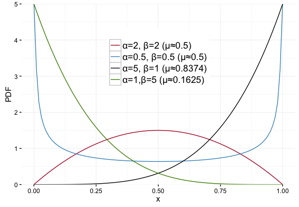
Figure 3. Probability density functions of four different beta distributions used in private ratings allocation.

4.3. Results

We evaluate our SP2 framework using accuracy-based as well as ranking-based metric. The 5-fold average RMSE and NDCG@10 scores (Liu et al., 2016) along with their corresponding standard deviations are reported in Table 4.3 for the MovieLens and Amazon Electronics datasets.

Table 2. Experimental results on MovieLens and Amazon Electronics datasets

Category	Method	Model Parameters	Movielens		Amazon Electronics
			RMSE	NDCG@10	RMSE	NDCG@10
20cmPeer-to-peer Based	Shokri et al. (FR)	#Peers$=10$	1.1624$\pm$0.00189	0.4873$\pm$0.0055	1.2216$\pm$0.01229	0.7757$\pm$0.00841
	Shokri et al. (SR)	#Peers$=10$	1.1624$\pm$0.00562	0.4891$\pm$0.00773	1.2048$\pm$0.00889	0.7774$\pm$0.00686
	Shokri et al. (SM)	#Peers$=10$	1.1447$\pm$0.00629	0.4922$\pm$0.0094	1.2028$\pm$0.00985	0.7748$\pm$0.00887
	Berkovsky et al.	#Peers$=40$	1.132$\pm$0.00411	0.4876$\pm$0.00599	1.3405$\pm$0.00562	0.7619$\pm$0.00756
Diff. Privacy	McSherry et al.	$\beta_{m}=15$	1.201$\pm$0.00675	0.4795$\pm$0.00911	1.1349$\pm$0.00664	0.7719$\pm$0.00675
20cmExtreme Baselines	Abs. Pessimistic	$k=100,\text{\#epochs}=20$	0.9632$\pm$0.00489	0.4132$\pm$0.00661	0.9788$\pm$0.00368	0.7379$\pm$0.00535
	Abs. Optimistic	$k=100,\text{\#epochs}=20$	0.8923$\pm$0.00576	0.5426$\pm$0.0072	0.9538$\pm$0.00955	0.788$\pm$0.00818
20cmClassic Collaborative Filtering	Only Public (H1)	$\alpha=2,\beta=2,\mu=0.48$	0.9183$\pm$0.00725	0.545$\pm$0.00726	0.971$\pm$0.00516	0.7892$\pm$0.00334
		$\alpha=0.5,\beta=0.5,\mu=0.48$	0.925$\pm$0.0075	0.5468$\pm$0.00688	0.9775$\pm$0.00455	0.788$\pm$0.00204
		$\alpha=5,\beta=1,\mu=0.82$	0.9518$\pm$0.00822	0.5363$\pm$0.00727	0.9957$\pm$0.00763	0.7738$\pm$0.00233
		$\alpha=1,\beta=5,\mu=0.17$	0.9033$\pm$0.00641	0.5534$\pm$0.00179	0.96$\pm$0.00411	0.7955$\pm$0.00446
	Only Public (H2)	$\alpha=2,\beta=2,\mu=0.48$	0.9206$\pm$0.00328	0.5391$\pm$0.00179	0.9692$\pm$0.00895	0.787$\pm$0.00463
		$\alpha=0.5,\beta=0.5,\mu=0.48$	0.9287$\pm$0.00228	0.528$\pm$0.00596	0.969$\pm$0.00931	0.7853$\pm$0.00242
		$\alpha=5,\beta=1,\mu=0.82$	0.9522$\pm$0.00213	0.517$\pm$0.00797	0.9851$\pm$0.00808	0.7718$\pm$0.00517
		$\alpha=1,\beta=5,\mu=0.17$	0.9063$\pm$0.00294	0.5466$\pm$0.00212	0.9581$\pm$0.00946	0.7929$\pm$0.00456
20cmSelective Privacy Preserving (SP2)	Naive (H1)	$\alpha=2,\beta=2,\mu=0.48$	0.9051$\pm$0.00654	0.5558$\pm$0.00511	0.9613$\pm$0.00534	0.7991$\pm$0.00322
		$\alpha=0.5,\beta=0.5,\mu=0.48$	0.9072$\pm$0.00873	0.5542$\pm$0.00727	0.9641$\pm$0.00555	0.7978$\pm$0.0012
		$\alpha=5,\beta=1,\mu=0.82$	0.9316$\pm$0.0088	0.5444$\pm$0.00666	0.9808$\pm$0.00733	0.7868$\pm$0.00297
		$\alpha=1,\beta=5,\mu=0.17$	0.8953$\pm$0.00688	0.5594$\pm$0.00696	0.9526$\pm$0.00525	0.8048$\pm$0.00318
	Naive (H2)	$\alpha=2,\beta=2,\mu=0.48$	0.907$\pm$0.00377	0.5514$\pm$0.00123	0.9589$\pm$0.00921	0.7977$\pm$0.00378
		$\alpha=0.5,\beta=0.5,\mu=0.48$	0.914$\pm$0.00302	0.5383$\pm$0.00491	0.9603$\pm$0.00937	0.793$\pm$0.00222
		$\alpha=5,\beta=1,\mu=0.82$	0.9316$\pm$0.00215	0.5274$\pm$0.00802	0.9705$\pm$0.00795	0.7824$\pm$0.00459
		$\alpha=1,\beta=5,\mu=0.17$	0.8946$\pm$0.0032	0.5532$\pm$0.00306	0.9517$\pm$0.00949	0.8034$\pm$0.00411
	Clustering (H1)	$\alpha=2,\beta=2,\mu=0.48$	0.9165$\pm$0.00766	0.5457$\pm$0.00695	0.966$\pm$0.00565	0.7893$\pm$0.00353
		$\alpha=0.5,\beta=0.5,\mu=0.48$	0.9146$\pm$0.01183	0.5494$\pm$0.00795	0.9695$\pm$0.00774	0.7876$\pm$0.00309
		$\alpha=5,\beta=1,\mu=0.82$	0.9387$\pm$0.00854	0.5366$\pm$0.00681	0.9847$\pm$0.00741	0.7736$\pm$0.00241
		$\alpha=1,\beta=5,\mu=0.17$	0.9037$\pm$0.00634	0.5538$\pm$0.00206	0.958$\pm$0.0048	0.7945$\pm$0.00373
	Clustering (H2)	$\alpha=2,\beta=2,\mu=0.48$	0.9183$\pm$0.00395	0.5401$\pm$0.00172	0.9653$\pm$0.00924	0.7871$\pm$0.00464
		$\alpha=0.5,\beta=0.5,\mu=0.48$	0.9249$\pm$0.00206	0.5287$\pm$0.00598	0.9651$\pm$0.00938	0.7852$\pm$0.00228
		$\alpha=5,\beta=1,\mu=0.82$	0.9405$\pm$0.00166	0.5174$\pm$0.00718	0.9757$\pm$0.00812	0.7716$\pm$0.00528
		$\alpha=1,\beta=5,\mu=0.17$	0.9047$\pm$0.00319	0.5473$\pm$0.00121	0.9566$\pm$0.00971	0.7926$\pm$0.00436
	Joint Opt. (H1)	$\alpha=2,\beta=2,\mu=0.48$	0.9051$\pm$0.00654	0.556$\pm$0.00502	0.9612$\pm$0.00533	0.7989$\pm$0.00315
		$\alpha=0.5,\beta=0.5,\mu=0.48$	0.9072$\pm$0.00873	0.5537$\pm$0.00735	0.964$\pm$0.00556	0.7975$\pm$0.00098
		$\alpha=5,\beta=1,\mu=0.82$	0.9316$\pm$0.0088	0.5447$\pm$0.00646	0.9808$\pm$0.00734	0.7869$\pm$0.00338
		$\alpha=1,\beta=5,\mu=0.17$	0.8953$\pm$0.00689	0.5592$\pm$0.00706	0.9526$\pm$0.00524	0.8045$\pm$0.00318
	Joint Opt. (H2)	$\alpha=2,\beta=2,\mu=0.48$	0.907$\pm$0.00377	0.551$\pm$0.00095	0.9589$\pm$0.0092	0.7978$\pm$0.00371
		$\alpha=0.5,\beta=0.5,\mu=0.48$	0.914$\pm$0.00302	0.5383$\pm$0.00507	0.9602$\pm$0.00939	0.793$\pm$0.0022
		$\alpha=5,\beta=1,\mu=0.82$	0.9319$\pm$0.00241	0.5278$\pm$0.00851	0.9705$\pm$0.00792	0.782$\pm$0.00479
		$\alpha=1,\beta=5,\mu=0.17$	0.8947$\pm$0.0032	0.5533$\pm$0.00289	0.9517$\pm$0.0095	0.8034$\pm$0.00423

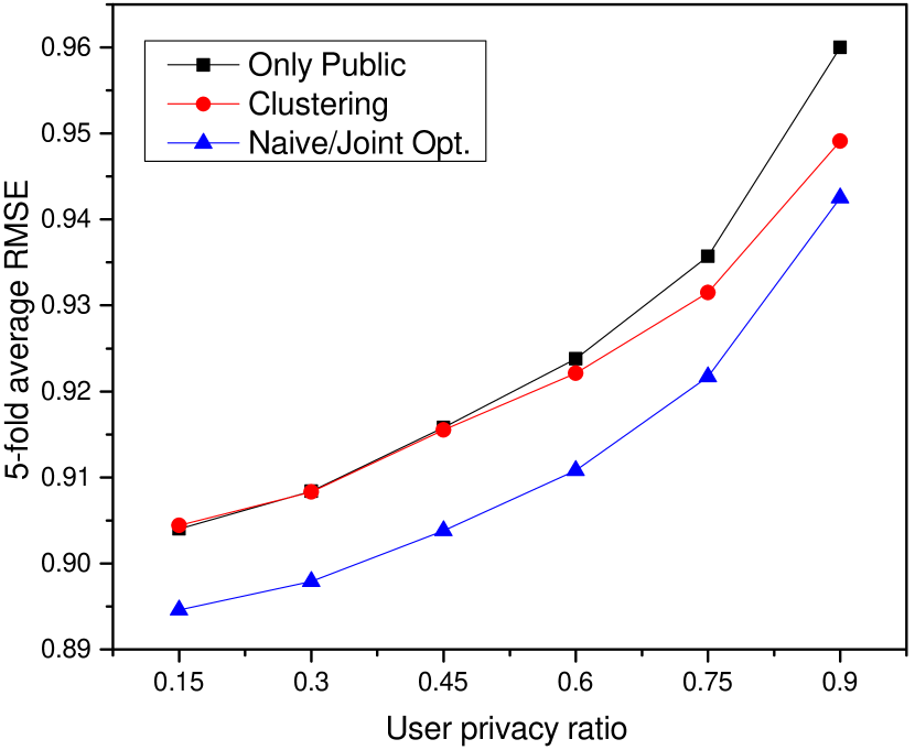
(a) RMSE comparison

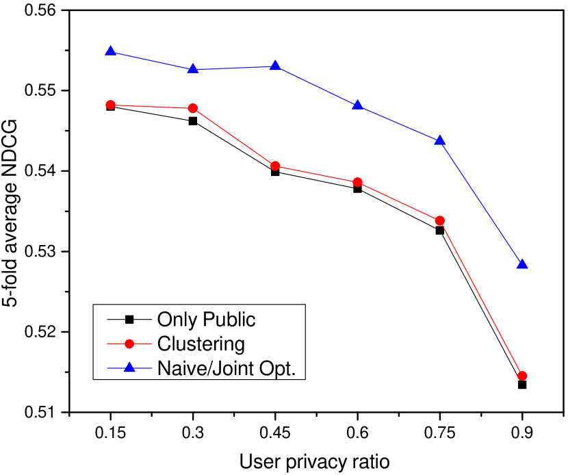
(b) NDCG comparison

Figure 4. Performance comparison among various baselines for different user privacy ratios on MovieLens dataset.

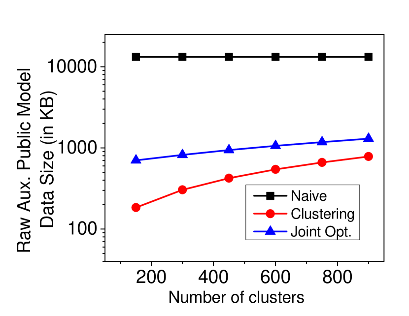
(a) Aux. data size comparison

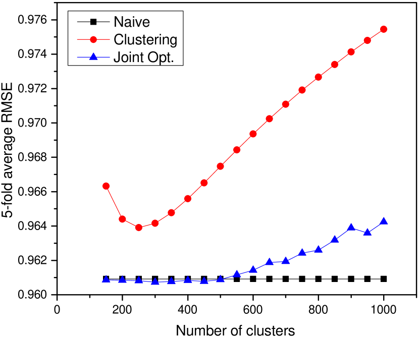
(b) RMSE comparison

Figure 5. Comparing SP2 implementations for different number of clusters on Amazon Electronics dataset (preprocessed using mostly balanced beta distribution and H1).

As indicated by the results in Table 4.3, the peer-to-peer based techniques and the differential privacy method, which attempt to ensure complete user privacy from the central recommender system, end up performing worse than the standard only public baseline due to the data obfuscation policies. In addition, the fully decentralized approach in (Berkovsky et al., 2007) is not scalable due to the limited number of trusted peers. In the same vein, the distributed aggregation approaches in (Shokri et al., 2009) suffer from poor performance as the number of peers increases due to higher obfuscation; however, lowering the number of peers risks significant privacy breach by the central recommender system. Table 4.3 further summarizes that our joint optimization approach (with only top-3 cluster weights) performs as good as the naive approach. Our clustering approach for SP2 framework, performs worse than naive and joint optimization but is largely better than the only public baseline across both evaluation metrics. Unless otherwise mentioned in the table, $P$-value for all results related to SP2 framework (computed using two-tailed test with respect to only public baseline) is less than $0.001$. As evident from the table, our results hold across both the hypotheses. However, the performance of all the implementations improve as the privacy ratio reduces. This is further demonstrated through figures 3(a) and 3(b) which plot the RMSE and NDCG values respectively against varying average user privacy ratio across all users. Finally, figures 4(a) and 4(b) present an ablation study that studies the performance and communication cost for different SP2 frameworks with varying number of clusters. The naive method has the best performance but requires the largest auxiliary model data. The joint optimization technique require an order of magnitude less data than the naive one but can reach the same performance for an optimal number of clusters.

5. Survey

We conducted a survey to gauge public interest in using our SP2 framework. In total, 74 users responded, of which 74% were male and 24% were female. 92% of our respondents were within the age bracket $(18-30)$. In our survey, we found that 57% of the participants do not rate items on any platform, whereas around 20% of the users provide a lot of ratings. About 48% of the respondents claim they hesitate to rate an item because they do not want to share their opinion publicly or because they do not trust the platform. The last two questions in our survey were aimed at estimating how likely a user is to provide a rating, if he/she can use our selective privacy preserving framework. When users were asked if they would rate more items privately on their device, if it guarantees to improve the quality of their recommendations, about 56% of the users responded affirmatively, while 22% said ‘maybe’ and 22% responded with a disagreement. The responses to this survey indicate that an overwhelming majority of users are willing to use our proposed selective privacy preserving framework in order to improve their recommendations as well as safeguard their private information.

6. Related Work

Privacy preserving recommender systems has been well explored in the literature. Peer-to-peer (P2P) techniques (Berkovsky et al., 2007) are largely meant to protect users from untrusted servers. However, they also require users to share their private information with peers, which is a privacy breach in itself. In addition, P2P architectures lack scalability due to limited number of trusted peers and are vulnerable to malicious interferences by rogue actors. Differential privacy methods (McSherry and Mironov, 2009) provide theoretical privacy guarantees for all users, but can also adversely impact the performance of the recommender systems due to data obfuscation.

The related literature also comprises of cryptology (Zhan et al., 2008) based techniques that approach the problem little differently. For example, Zhan et al.(Zhan et al., 2008) used “homomorphic encryption” to integrate multiple sources of encrypted user ratings in a privacy preserving manner. However, the extreme computation time and scalability issues associated with homomorphic encryption pose a serious practicality question (Naehrig et al., 2011), even for moderate size datasets.

Lastly, recent federated machine learning approaches (Konećný et al., 2016) have proposed privacy-preserving techniques to build machine learning models using secure aggregation protocol (Bonawitz et al., 2017). However, in case of CF algorithms, this would require a user to share an update (in encrypted form) performed on an item factor locally. In our case, this means that the server would be able to identify from the encrypted updates, which items the user had rated privately, even though the exact ratings remain unknown. This itself constitutes a serious privacy breach (Chow et al., 2012; Advokat, 1987; McCabe, 2012). Hence, in our SP2 framework, no private user information is ever uploaded or communicated.

7. Conclusion

In this paper, we proposed a novel selective privacy preserving (SP2) paradigm for CF based recommender systems that allows users to keep a portion of their ratings private, meanwhile delivering better recommendations, as compared to other privacy preserving techniques. We have demonstrated the efficacy of our approach under different configurations by comparing it against other baselines on two real datasets. Finally, our framework empowers users to define their own privacy policy by determining which ratings should be private and which ones should be public.

References

- (1)
- Advokat (1987) Stephen Advokat. 1987. Publication of Bork’s video rentals raises privacy issue. Chicago Tribune (1987).
- Arthur and Vassilvitskii (2007) David Arthur and Sergei Vassilvitskii. 2007. K-means++: The Advantages of Careful Seeding. In Proceedings of the Eighteenth Annual ACM-SIAM Symposium on Discrete Algorithms (SODA ’07). Society for Industrial and Applied Mathematics, 1027–1035. http://dl.acm.org/citation.cfm?id=1283383.1283494
- Berkovsky et al. (2007) Shlomo Berkovsky, Yaniv Eytani, Tsvi Kuflik, and Francesco Ricci. 2007. Enhancing Privacy and Preserving Accuracy of a Distributed Collaborative Filtering. In Proceedings of the 2007 ACM Conference on Recommender Systems (RecSys ’07). ACM, 9–16. https://doi.org/10.1145/1297231.1297234
- Bloom (1970) Burton H. Bloom. 1970. Space/Time Trade-offs in Hash Coding with Allowable Errors. Commun. ACM 13, 7 (July 1970), 422–426. https://doi.org/10.1145/362686.362692
- Bonawitz et al. (2017) Keith Bonawitz, Vladimir Ivanov, Ben Kreuter, Antonio Marcedone, H. Brendan McMahan, Sarvar Patel, Daniel Ramage, Aaron Segal, and Karn Seth. 2017. Practical Secure Aggregation for Privacy Preserving Machine Learning. Cryptology ePrint Archive, Report 2017/281. (2017). https://eprint.iacr.org/2017/281.
- Canny (2002) John Canny. 2002. Collaborative Filtering with Privacy via Factor Analysis. In Proceedings of the 25th Annual International ACM SIGIR Conference on Research and Development in Information Retrieval (SIGIR ’02). ACM, 238–245. https://doi.org/10.1145/564376.564419
- Chow et al. (2012) Richard Chow, Manas A. Pathak, and Cong Wang. 2012. A Practical System for Privacy-Preserving Collaborative Filtering. In 12th IEEE International Conference on Data Mining Workshops, ICDM Workshops, Brussels, Belgium, December 10, 2012. 547–554. https://doi.org/10.1109/ICDMW.2012.84
- Das et al. (2017) Ariyam Das, Ishan Upadhyaya, Xiangrui Meng, and Ameet Talwalkar. 2017. Collaborative Filtering As a Case-Study for Model Parallelism on Bulk Synchronous Systems. In Proceedings of the 2017 ACM on Conference on Information and Knowledge Management (CIKM ’17). ACM, 969–977. https://doi.org/10.1145/3132847.3132862
- Ge et al. (2016) Rong Ge, Jason D. Lee, and Tengyu Ma. 2016. Matrix Completion Has No Spurious Local Minimum. In Proceedings of the 30th International Conference on Neural Information Processing Systems (NIPS’16). Curran Associates Inc., 2981–2989. http://dl.acm.org/citation.cfm?id=3157382.3157431
- Grodzevich and Romanko (2006) Oleg Grodzevich and Oleksandr Romanko. 2006. Normalization and other topics in multi-objective optimization. In Proceedings of the Fields-MITACS Industrial Problems Workshop.
- Harper and Konstan (2015) F. Maxwell Harper and Joseph A. Konstan. 2015. The MovieLens Datasets: History and Context. ACM Trans. Interact. Intell. Syst. 5, 4, Article 19 (Dec. 2015), 19 pages. https://doi.org/10.1145/2827872
- Kanungo et al. (2002) Tapas Kanungo, David M. Mount, Nathan S. Netanyahu, Christine D. Piatko, Ruth Silverman, and Angela Y. Wu. 2002. An Efficient k-Means Clustering Algorithm: Analysis and Implementation. IEEE Trans. Pattern Anal. Mach. Intell. 24, 7 (July 2002), 881–892. https://doi.org/10.1109/TPAMI.2002.1017616
- Karydi and Margaritis (2016) Efthalia Karydi and Konstantinos Margaritis. 2016. Parallel and Distributed Collaborative Filtering: A Survey. ACM Comput. Surv. 49, 2, Article 37 (Aug. 2016), 41 pages. https://doi.org/10.1145/2951952
- Keuper and Pfreundt (2015) Janis Keuper and Franz-Josef Pfreundt. 2015. Asynchronous Parallel Stochastic Gradient Descent: A Numeric Core for Scalable Distributed Machine Learning Algorithms. In Proceedings of the Workshop on Machine Learning in High-Performance Computing Environments (MLHPC ’15). ACM, Article 1, 11 pages. https://doi.org/10.1145/2834892.2834893
- Konećný et al. (2016) Jakub Konećný, H. Brendan McMahan, Daniel Ramage, and Peter Richtarik. 2016. Federated Optimization: Distributed Machine Learning for On-Device Intelligence. (2016). https://arxiv.org/abs/1610.02527
- Koren et al. (2009) Yehuda Koren, Robert Bell, and Chris Volinsky. 2009. Matrix Factorization Techniques for Recommender Systems. Computer 42, 8 (Aug. 2009), 30–37. https://doi.org/10.1109/MC.2009.263
- Lee and Seung (2000) Daniel D. Lee and H. Sebastian Seung. 2000. Algorithms for Non-negative Matrix Factorization. In Proceedings of the 13th International Conference on Neural Information Processing Systems (NIPS’00). MIT Press, 535–541. http://dl.acm.org/citation.cfm?id=3008751.3008829
- Lee et al. (2016) Jason D. Lee, Max Simchowitz, Michael I. Jordan, and Benjamin Recht. 2016. Gradient Descent Only Converges to Minimizers. In 29th Annual Conference on Learning Theory (Proceedings of Machine Learning Research), Vitaly Feldman, Alexander Rakhlin, and Ohad Shamir (Eds.), Vol. 49. PMLR, 1246–1257. http://proceedings.mlr.press/v49/lee16.html
- Li et al. (2016) Mu Li, Ziqi Liu, Alexander J. Smola, and Yu-Xiang Wang. 2016. DiFacto: Distributed Factorization Machines. In Proceedings of the Ninth ACM International Conference on Web Search and Data Mining (WSDM ’16). ACM, 377–386. https://doi.org/10.1145/2835776.2835781
- Lin (2007) Chih-Jen Lin. 2007. Projected Gradient Methods for Nonnegative Matrix Factorization. Neural Comput. 19, 10 (Oct. 2007), 2756–2779. https://doi.org/10.1162/neco.2007.19.10.2756
- Liu et al. (2017) Yuan Liu, Usman Shittu Chitawa, Guibing Guo, Xingwei Wang, Zhenhua Tan, and Shuang Wang. 2017. A Reputation Model for Aggregating Ratings Based on Beta Distribution Function. In Proceedings of the 2nd International Conference on Crowd Science and Engineering (ICCSE’17). ACM, 77–81. https://doi.org/10.1145/3126973.3126992
- Liu et al. (2016) Yanchi Liu, Chuanren Liu, Bin Liu, Meng Qu, and Hui Xiong. 2016. Unified Point-of-Interest Recommendation with Temporal Interval Assessment. In Proceedings of the 22Nd ACM SIGKDD International Conference on Knowledge Discovery and Data Mining (KDD ’16). ACM, New York, NY, USA, 1015–1024. https://doi.org/10.1145/2939672.2939773
- Marais and Bharat (1997) Hannes Marais and Krishna Bharat. 1997. Supporting Cooperative and Personal Surfing with a Desktop Assistant. In Proceedings of the 10th Annual ACM Symposium on User Interface Software and Technology (UIST ’97). ACM, 129–138. https://doi.org/10.1145/263407.263531
- McAuley et al. (2015) Julian McAuley, Christopher Targett, Qinfeng Shi, and Anton van den Hengel. 2015. Image-Based Recommendations on Styles and Substitutes. In Proceedings of the 38th International ACM SIGIR Conference on Research and Development in Information Retrieval (SIGIR ’15). ACM, 43–52. https://doi.org/10.1145/2766462.2767755
- McCabe (2012) Kathryn E. McCabe. 2012. Just you and me and netflix makes three: Implications for allowing frictionless sharing of personally identifiable information under the video privacy protection act. J. Intell. Prop. L. (2012).
- McSherry and Mironov (2009) Frank McSherry and Ilya Mironov. 2009. Differentially Private Recommender Systems: Building Privacy into the Netflix Prize Contenders. In Proceedings of the 15th ACM SIGKDD International Conference on Knowledge Discovery and Data Mining (KDD ’09). ACM, 627–636. https://doi.org/10.1145/1557019.1557090
- Meng et al. (2016) Xiangrui Meng, Joseph Bradley, Burak Yavuz, Evan Sparks, Shivaram Venkataraman, Davies Liu, Jeremy Freeman, DB Tsai, Manish Amde, Sean Owen, Doris Xin, Reynold Xin, Michael J. Franklin, Reza Zadeh, Matei Zaharia, and Ameet Talwalkar. 2016. MLlib: Machine Learning in Apache Spark. J. Mach. Learn. Res. 17, 1 (Jan. 2016), 1235–1241. http://dl.acm.org/citation.cfm?id=2946645.2946679
- Mishra and Reddy (2016) Sonu K. Mishra and Manoj Reddy. 2016. A Bottom-up Approach to Job Recommendation System. In Proceedings of the Recommender Systems Challenge (RecSys Challenge ’16). ACM, Article 4, 4 pages. https://doi.org/10.1145/2987538.2987546
- Naehrig et al. (2011) Michael Naehrig, Kristin Lauter, and Vinod Vaikuntanathan. 2011. Can Homomorphic Encryption Be Practical?. In Proceedings of the 3rd ACM Workshop on Cloud Computing Security Workshop (CCSW ’11). ACM, New York, NY, USA, 113–124. https://doi.org/10.1145/2046660.2046682
- Narayanan and Shmatikov (2008) Arvind Narayanan and Vitaly Shmatikov. 2008. Robust De-anonymization of Large Sparse Datasets. In Proceedings of the 2008 IEEE Symposium on Security and Privacy (SP ’08). IEEE Computer Society, 111–125. https://doi.org/10.1109/SP.2008.33
- Oh et al. (2015) Jinoh Oh, Wook-Shin Han, Hwanjo Yu, and Xiaoqian Jiang. 2015. Fast and Robust Parallel SGD Matrix Factorization. In Proceedings of the 21th ACM SIGKDD International Conference on Knowledge Discovery and Data Mining (KDD ’15). ACM, 865–874. https://doi.org/10.1145/2783258.2783322
- Schelter et al. (2013) Sebastian Schelter, Christoph Boden, Martin Schenck, Alexander Alexandrov, and Volker Markl. 2013. Distributed Matrix Factorization with Mapreduce Using a Series of Broadcast-joins. In Proceedings of the 7th ACM Conference on Recommender Systems (RecSys ’13). ACM, 281–284. https://doi.org/10.1145/2507157.2507195
- Shokri et al. (2009) Reza Shokri, Pedram Pedarsani, George Theodorakopoulos, and Jean-Pierre Hubaux. 2009. Preserving Privacy in Collaborative Filtering Through Distributed Aggregation of Offline Profiles. In Proceedings of the Third ACM Conference on Recommender Systems (RecSys ’09). ACM, 157–164. https://doi.org/10.1145/1639714.1639741
- Takács et al. (2008) Gábor Takács, István Pilászy, Bottyán Németh, and Domonkos Tikk. 2008. Matrix Factorization and Neighbor Based Algorithms for the Netflix Prize Problem. In Proceedings of the 2008 ACM Conference on Recommender Systems (RecSys ’08). ACM, 267–274. https://doi.org/10.1145/1454008.1454049
- Takács and Tikk (2012) Gábor Takács and Domonkos Tikk. 2012. Alternating Least Squares for Personalized Ranking. In Proceedings of the Sixth ACM Conference on Recommender Systems (RecSys ’12). ACM, 83–90. https://doi.org/10.1145/2365952.2365972
- Volkovs et al. (2017) Maksims Volkovs, Guangwei Yu, and Tomi Poutanen. 2017. DropoutNet: Addressing Cold Start in Recommender Systems. In Advances in Neural Information Processing Systems 30, I. Guyon, U. V. Luxburg, S. Bengio, H. Wallach, R. Fergus, S. Vishwanathan, and R. Garnett (Eds.). Curran Associates, Inc., 4964–4973. http://papers.nips.cc/paper/7081-dropoutnet-addressing-cold-start-in-recommender-systems.pdf
- Wu et al. (2016) Yao Wu, Xudong Liu, Min Xie, Martin Ester, and Qing Yang. 2016. CCCF: Improving Collaborative Filtering via Scalable User-Item Co-Clustering. In Proceedings of the Ninth ACM International Conference on Web Search and Data Mining (WSDM ’16). ACM, 73–82. https://doi.org/10.1145/2835776.2835836
- Xing (2015) Eric P. et al. Xing. 2015. Petuum: A New Platform for Distributed Machine Learning on Big Data. In Proceedings of the 21th ACM SIGKDD International Conference on Knowledge Discovery and Data Mining (KDD ’15). ACM, 1335–1344. https://doi.org/10.1145/2783258.2783323
- Zhan et al. (2008) Justin Zhan, I-Cheng Wang, Chia-Lung Hsieh, Tsan-sheng Hsu, Churn-Jung Liau, and Da-Wei Wang. 2008. Towards Efficient Privacy-preserving Collaborative Recommender Systems. In The 2008 IEEE International Conference on Granular Computing, GrC 2008, Hangzhou, China, 26-28 August 2008. 778–783. https://doi.org/10.1109/GRC.2008.4664769