Conservative Exploration using Interleaving

Abstract

In many practical problems, a learning agent may want to learn the best action in hindsight without ever taking a bad action, which is significantly worse than the default production action. In general, this is impossible because the agent has to explore unknown actions, some of which can be bad, to learn better actions. However, when the actions are combinatorial, this may be possible if the unknown action can be evaluated by interleaving it with the production action. We formalize this concept as learning in stochastic combinatorial semi-bandits with exchangeable actions. We design efficient learning algorithms for this problem, bound their $n$-step regret, and evaluate them on both synthetic and real-world problems. Our real-world experiments show that our algorithms can learn to recommend $K$ most attractive movies without ever violating a strict production constraint, both overall and subject to a diversity constraint.

1 Introduction

Recommender systems are an integral component of many industries, with applications in content personalization, advertising, and landing page design [24, 1, 6]. Multi-armed bandit algorithms provide adaptive techniques for content recommendation, and although theoretically well-understood, they have not been widely adopted in production systems [11, 25]. This is primarily due to concerns that the output of the bandit algorithm can be sub-optimal or even disastrous, especially when the algorithm explores sub-optimal arms. To address this issue, most industries have a static recommendation engine in production that has been well-optimized and tested over many years, and a promising new policy is often evaluated using A/B testing [26] by allocating a small percentage $\alpha$ of the traffic to the new policy. When the utilities of actions are independent, this is a reasonable solution that allows the new policy to explore non-aggressively.

Many recommendation problems, however, involve structured actions, such as ranked lists of items (movies, products, etc.). In such actions, the total utility of the action can be decomposed into the utilities of its individual items. Therefore, it is conceivable that the new policy can be evaluated in a controlled and principled fashion by interleaving items in the new and production actions, instead of splitting the traffic as is done in A/B testing. As a concrete example, consider the problem of recommending top-$K$ movies to a new visitor [12]. A company may have a production policy that recommends a default set of $K$ movies that performs reasonably well, but intends to test a new algorithm that promises to learn better movies. The A/B testing method would show the new algorithm’s recommendations to a visitor with probability $\alpha$. In the initial stages, the new algorithm is expected to explore a lot to learn, and may hurt engagement with the visitor who is shown a disastrous set of movies, just to learn that these movies are not good. However, an arguably better approach that does not hurt any visitor’s engagement as much and gathers the same feedback on average, is to show the default well-tested movies interleaved with $\alpha$ fraction of new recommendations. A recent study by Schnabel et al. [25] concluded that this latter approach is in fact better:

“These findings indicate that for improving recommendation systems in practice, it is preferable to mix a limited amount of exploration into every impression – as opposed to having a few impressions that do pure exploration.”

In this paper, we formalize the above idea and study the general case where actions are exchangeable, which is a mathematical formulation of the notion of interleaving. One fairly general and important class of exchangeable actions is the set of bases of a matroid, and this is the setting we focus on in our theorems and experiments. In particular, we study learning variants of maximizing an unknown modular function on a matroid subject to a conservative constraint.

In the recommendations problem discussed above, our conservative constraint requires that the recommendations always be above a certain baseline quality. The question we wish to answer is: what is the price of being this conservative? In this work, we answer this question and make five contributions. First, we introduce the idea of conservative multi-armed bandits in combinatorial action spaces, and formulate a conservative constraint that addresses the issues raised in Schnabel et al. [25]. Existing conservative constraints for multi-armed bandit problems fail in this aspect, and hence our constraint is more appropriate for combinatorial action spaces. Second, we propose interleaving as a solution, and show how it naturally leads to the idea of exchangeable action spaces. We precisely formulate an online learning problem - conservative interleaving bandits - in one such space, that of matroids. Third, we present Interleaving Upper Confidence Bound (${\tt I\mathchar 45\relax UCB}$), a computationally and sample-efficient algorithm for solving our problem. The algorithm satisfies our conservative constraint by design. Fourth, we prove gap-dependent upper bounds on its expected cumulative regret, and show that the regret scales logarithmically in the number of steps $n$, at most linearly in the number of items $L$, and at most quadratically in the number of items $K$ in any action. Finally, we evaluate ${\tt I\mathchar 45\relax UCB}$ on both synthetic and real-world problems. In the synthetic experiments, we validate an extra factor in our regret bounds, which is the price for being conservative. In the real-world experiments, we illustrate how to formulate and solve top-$K$ recommendation problems in our setting. To the best of our knowledge, this is the first work that studies conservatism in the context of combinatorial bandit problems.

2 Setting

We focus on linear reward functions and formulate our learning problem as a stochastic combinatorial semi-bandit [20, 14, 9], which we first review in Section 2.1. Stochastic combinatorial semi-bandits have been used for recommendation problems before [19, 18]. In Section 2.2, we motivate our notion of conservativeness, and suggest interleaving as a solution, which can be mathematically formulated using exchangeable action spaces. Finally, in Section 2.3, we show that actions that are bases of a matroid are exchangeable, and phrase our problem using the terminology of matroids. To simplify exposition, we write all random variables in bold. We use $[K]$ to denote the set $\{1,\dots,K\}$.

2.1 Stochastic Combinatorial Semi-Bandits

A stochastic combinatorial semi-bandit [20, 14, 9] is a tuple $(E,\mathcal{B},P)$, where $E=[L]$ is a finite set of $L$ items, $\mathcal{B}\subseteq\Pi_{K}(E)$ is a non-empty set of feasible subsets of $E$ of size $K$, and $P$ is a probability distribution over a unit cube $[0,1]^{E}$. Here $\Pi_{K}(E)$ is the set of all $K$-permutations of $E$.

Let $(\bm{w}_{t})_{t=1}^{n}$ be an i.i.d. sequence of $n$ weights drawn according to $P$, where $\bm{w}_{t}(e)$ is the weight of item $e\in E$ at time $t$. The learning agent interacts with our problem as follows. At time $t$, it takes an action $\bm{A}_{t}\in\mathcal{B}$, which is a set of items from $E$. The reward for taking the action is $f(\bm{A}_{t},\bm{w}_{t})$, where $f(A,w)=\sum_{e\in A}w(e)$ is the sum of the weights of items in $A$ in weight vector $w$. After taking action $\bm{A}_{t}$, the agent observes the weight $\bm{w}_{t}(e)$ for each item $e\in\bm{A}_{t}$. This model of feedback is known as semi-bandit [2].

The learning agent is evaluated by its expected $n$-step regret $R(n)=\mathbb{E}\!\left[\sum_{t=1}^{n}R(\bm{A}_{t},\bm{w}_{t})\right]$, where $R(\bm{A}_{t},\bm{w}_{t})=f(A_{\ast},\bm{w}_{t})-f(\bm{A}_{t},\bm{w}_{t})$ is the instantaneous stochastic regret of the agent at time $t$ and $A_{\ast}=\operatorname*{arg\,max\,}_{A\in\mathcal{B}}f(A,\bar{w})$ is the maximum weight action in hindsight.

2.2 Conservativeness and Exchangeable Actions

The idea of controlled exploration is not new. Wu et al. [29] studied conservatism in multi-armed bandits, and their learning agent is constrained to have its cumulative reward no worse than $1-\alpha$ of that of the default action. In this sense, their conservative constraint is cumulative. Roughly speaking, the constraint means that the learning agent can explore once in every $1/\alpha$ steps.

A/B testing can also be thought of as the solution to a constrained exploration problem where the constraint is instantaneous (instead of cumulative); here the constraint requires that the actions at any time be at least $(1-\alpha)$ good as the default action in expectation, where the expectation is taken over multiple runs of the A/B test.

When actions are combinatorial, as in the top-$K$ movie recommendation problem in Section 1, both these forms of conservatism allow the learning agent to occasionally take actions containing items that are all disastrous (for example, have very low popularity). We consider a stricter conservative constraint that explicitly forbids this possibility.

We state our conservative constraint next. Let $K$ be the number of items in any action. Let $B_{0}$ be the default baseline action, where $|B_{0}|=K$. Our constraint requires that at any time $t$, the action $\bm{A}_{t}$ should be at least as good as the baseline set $B_{0}$, in the sense that most items in $\bm{A}_{t}$ are at least as good or better than those in $B_{0}$. Mathematically, we require that there exists a bijection $\rho_{\bm{A}_{t},B_{0}}:\bm{A}_{t}\rightarrow B_{0}$ such that

$$\sum_{e\in\bm{A}_{t}}\mathbbm{1}\!\left(\bar{w}(e)\geq\bar{w}(\rho_{\bm{A}_{t},B_{0}}(e))\right)\geq(1-\alpha)K$$ (1)

holds with a high probability at any time $t$. That is, the items in $\bm{A}_{t}$ and $B_{0}$ can be matched such that no more than $\alpha$ fraction of the items in $\bm{A}_{t}$ has a lower expected reward than those in $B_{0}$. For simplicity of exposition, we only consider the special case of $\alpha=1/K$ in this work. We discuss the case $\alpha>1/K$ in Section 4.3.

Given an algorithm that explores and suggests new actions that could potentially be disastrous, a simple way to satisfy (1) is to interleave most items from the default action with a few from the new action. This is possible if the set of feasible actions $\mathcal{B}\subseteq 2^{E}$ is exchangeable, which we define next.

Definition 1.

A set $\mathcal{B}\subseteq 2^{E}$ is exchangeable if for any two actions $A_{1},A_{2}\in\mathcal{B}$, there exists a bijection $\rho_{A_{1},A_{2}}:A_{1}\rightarrow A_{2}$ such that

$$\forall\,e\in A_{1}:A_{1}\setminus\{e\}\cup\{\rho_{A_{1},A_{2}}(e)\}\in\mathcal{B}\,.$$ (2)

In our motivating top-$K$ movie recommendation example, $A_{1}$ is the default action (recommendation) and $A_{2}$ is the new action, and $|A_{1}|=|A_{2}|=K$. If the action space is exchangeable, we can explore all items in a new action $A_{2}$ over $K$ time steps by taking $K$ interleaved actions. Each interleaved action substitutes an item $e\in A_{1}$ with the item $\rho_{A_{1},A_{2}}(e)\in A_{2}$.

2.3 Conservative Interleaving Bandits

In this section, we consider an important exchangeable action space, the bases of a matroid. A matroid $M$ is a pair $(E,\mathcal{B})$ where $E=[L]$ is a finite set, and $\mathcal{B}\subseteq\Pi_{K}(E)$ is a collection of subsets of $E$ called bases [28]. $K$ is called the rank of the matroid.

Matroids have many interesting properties [22]; the one that is relevant to our work is the bijective exchange lemma for matroids [7], which states that the collection $\mathcal{B}$ is exchangeable.

Lemma 1 (Bijective Exchange Lemma).

For any two bases $B_{1},B_{2}\in\mathcal{B}$, there exists a bijection $\rho_{B_{1},B_{2}}:B_{1}\rightarrow B_{2}$ such that $(B_{1}\setminus\{e\})\cup\{\rho_{B_{1},B_{2}}(e)\}$ is a basis for any $e\in B_{1}$.

The recommendations for the top-$K$ movie problem in Section 1 are bases of a uniform matroid, which is a matroid whose items $E$ are movies and whose feasible sets are all $K$-permutations of these items, i.e., $\mathcal{B}=\Pi_{K}(E)$. One can also enforce diversity in the recommendations by formulating actions as the feasible set of a partition matroid, which is defined as follows. Let $\mathcal{P}_{1},\dots,\mathcal{P}_{K}$ be a partition of $[L]$. The feasible set of the partition matroid is $\mathcal{B}=\{A\in\Pi_{K}([L]):A(1)\in\mathcal{P}_{1},\dots,A(K)\in\mathcal{P}_{K}\}$. The members of the partition in this case correspond to the movie categories, and the partition matroid ensures that the recommended movies contain a movie from every category. In both the above matroids, $\rho_{A,B}$ maps the $k$-th item in $A$, $A(k)$, to the $k$-th item in $B$, $B(k)$. We study both of these examples in our experiments (Section 5). In addition to these examples, many important combinatorial optimization problems can be formulated as optimization on a matroid.

We formulate our learning problem using the terminology of matroids as a conservative interleaving bandit. A conservative interleaving bandit is a tuple $(E,\mathcal{B},P,B_{0},\alpha)$, where $E=[L]$ is a set of items, $\mathcal{B}\subseteq\Pi_{K}(E)$ is the collection of bases, $P$ is a probability distribution over the weights $\bm{w}\in\mathbb{R}^{L}$ of items $E$, the input baseline set $B_{0}\in\mathcal{B}$ is a basis, and $\alpha\in[0,1]$ is a tolerance parameter.

We assume that the matroid $(E,\mathcal{B})$, input baseline set $B_{0}$, and tolerance $\alpha$ are known and that the distribution $P$ is unknown. Without loss of generality, we assume that the support of $P$ is a bounded subset of $[0,1]^{L}$. We denote the expected weights of items by $\bar{w}=\mathbb{E}[\bm{w}]$.

3 Algorithm

Learning in conservative interleaving bandits is non-trivial. For instance, one cannot simply construct exploratory sets $\bm{D}_{t}$ using a non-conservative matroid bandit algorithm [18, 27], and then take actions $\bm{A}_{t}$ containing $(1-\alpha)$ fraction of items from the initial baseline set $B_{0}$ and the remaining items from $\bm{D}_{t}$. If the set $B_{0}$ contains sub-optimal items, the regret of this policy is linear since its actions never converge to the optimal action $A^{\ast}$.

In this section, we introduce our Interleaving Upper Confidence Bound (${\tt I\mathchar 45\relax UCB}$) algorithm which achieves sub-linear regret by maintaining a baseline set $\bm{B}_{t}$ which continuously improves over the initial baseline set $B_{0}$ with high probability. We present two variants of the algorithm: one where the agent knows the expected rewards of the input baseline set $\{\bar{w}(e):e\in B_{0}\}$, which we call ${\tt I\mathchar 45\relax UCB1}$; and one where the learner does not know them, which we call ${\tt I\mathchar 45\relax UCB2}$. The expected rewards of items in $B_{0}$ may be known in practice, for instance if the baseline policy has been deployed for a while. We refer to the common aspects of both algorithms as ${\tt I\mathchar 45\relax UCB}$.

The pseudocode of both algorithms is in Algorithm 1. We highlight differences in comments. Recall that $K$ is the rank of the matroid, or equivalently the number of items in any action. ${\tt I\mathchar 45\relax UCB}$ operates in rounds, which are indexed by $t$, and takes $K$ actions in each round. We assume that ${\tt I\mathchar 45\relax UCB}$ has access to an oracle MaxBasis that takes in a matroid and a vector of weights $w\in[L]$, and returns the maximum weight basis with respect to the weights $w$. MaxBasis is a greedy algorithm for matroids and hence can run in $O(L\log L)$ time [13].

Each round has three stages. In the first stage (lines $5$–$8$), ${\tt I\mathchar 45\relax UCB}$ computes upper confidence bounds (UCBs) $\bm{U}_{t}\in(\mathbb{R}^{+})^{E}$ and lower confidence bounds (LCBs) $\bm{L}_{t}\in(\mathbb{R}^{+})^{E}$ on the rewards of all items. For any item $e\in E$, let

$$\bm{U}_{t}(e)=\hat{\bm{w}}_{\bm{T}_{t-1}(e)}(e)+c_{n,\bm{T}_{t-1}(e)},\qquad\bm{L}_{t}(e)=\max\{\hat{\bm{w}}_{\bm{T}_{t-1}(e)}(e)-c_{n,\bm{T}_{t-1}(e)},0\}$$ (3)

where $\hat{\bm{w}}_{s}(e)$ is the average of $s$ observed weights of item $e$, $\bm{T}_{t}(e)$ is the number of times item $e$ has been observed in $t$ steps, and

$$c_{n,s}=\sqrt{1.5\log(n)/s}$$ (4)

is the radius of a confidence interval around $\hat{\bm{w}}_{s}(e)$ such that $\bar{w}(e)\in[\hat{\bm{w}}_{s}(e)-c_{n,s},\hat{\bm{w}}_{s}(e)+c_{n,s}]$ holds with a high probability. We adopt UCB1 confidence intervals [3] to simplify analysis, but it is possible to use tighter ${\tt KL\mathchar 45\relax UCB}$ confidence intervals [15].

Algorithm 1 ${\tt I\mathchar 45\relax UCB}$ for conservative interleaving bandits.

1:  Input: Set of items $E$, Collection of exchangeable actions $\mathcal{B}$, baseline action $B_{0}\in\mathcal{B}$

2:  

3:  Observe $\bm{w}_{0}\sim P$, $\forall\,e\in E:$ $\bm{T}_{0}(e)\leftarrow 1,\hat{\bm{w}}_{0}(e)\leftarrow\bm{w}_{0}(e)$ // Initialization

4:  

5:  for $t=1,2,\dots$ do

6:     for $e\in E$ do {// Compute UCBs and LCBs}

7:        $\bm{U}_{t}(e)=\hat{\bm{w}}_{\bm{T}_{t-1}(e)}(e)+c_{n,\bm{T}_{t-1}(e)}$

8:        $\bm{L}_{t}(e)=\max\{\hat{\bm{w}}_{\bm{T}_{t-1}(e)}(e)-c_{n,\bm{T}_{t-1}(e)},0\}$

9:     

10:     $\bm{D}_{t}\leftarrow$MaxBasis$((E,\mathcal{B}),\,\bm{U}_{t})$ // Compute decision set

11:     

12:     for $e\in B_{0}$ do {// Compute baseline set}

13:        if $\bar{w}(e)$ is known then {// ${\tt I\mathchar 45\relax UCB}1$}

14:           $\bm{v}_{t}(e)\leftarrow\bar{w}(e)$

15:        else {// ${\tt I\mathchar 45\relax UCB}2$}

16:           $\bm{v}_{t}(e)\leftarrow\bm{U}_{t}(e)$

17:     for $e\in E\setminus B_{0}$ do

18:        $\bm{v}_{t}(e)\leftarrow\bm{L}_{t}(e)$

19:     $\bm{B}_{t}\leftarrow$MaxBasis$((E,\mathcal{B}),\,\bm{v}_{t})$

20:     

21:     // Take $K$ combined actions of $\bm{D}_{t}$ and $\bm{B}_{t}$

22:     Let $\bm{\rho}_{t}:\bm{B}_{t}\rightarrow\bm{D}_{t}$ be the bijection in Lemma 1

23:     for $e\in\bm{B}_{t}$ do

24:        Take action $\bm{A}_{t}=\bm{B}_{t}\setminus\{e\}\cup\{\bm{\rho}_{t}(e)\}$

25:        Observe $\{\bm{w}_{t}(e):e\in\bm{A}_{t}\}$, where $\bm{w}_{t}\sim P$

26:        Update statistics $\hat{\bm{w}}$ and $\bm{T}$

In line $10$, ${\tt I\mathchar 45\relax UCB}$ chooses a decision set $\bm{D}_{t}$ which is the maximum weight basis with respect to $\bm{U}_{t}$, an optimistic estimate of $\bar{w}$. The same approach was used in Optimistic Matroid Maximization (OMM) of Kveton et al. [18]. However, unlike OMM, we cannot take action $\bm{D}_{t}$ because this action may not satisfy our conservative constraint in (1).

In the second stage (lines $12$–$19$), ${\tt I\mathchar 45\relax UCB}$ computes a baseline set $\bm{B}_{t}$ which improves over the input baseline set $B_{0}$ in each item with a high probability. The set $\bm{B}_{t}$ is the maximum weight basis with respect to weights $\bm{v}_{t}$, which are chosen as follows. For items $e\in B_{0}$, we set $\bm{v}_{t}(e)=\bar{w}(e)$ if $\bar{w}(e)$ is known, and $\bm{v}_{t}(e)=\bm{U}_{t}(e)$ if it is not. For items $e\in E\setminus B_{0}$, we set $\bm{v}_{t}(e)=\bm{L}_{t}(e)$. This setting guarantees that an item $e\in E\setminus B_{0}$ is selected over an item $e^{\prime}\in B_{0}$ only if its expected reward is higher than that of item $e^{\prime}$ with a high probability.

In the last stage (lines $22$–$26$), ${\tt I\mathchar 45\relax UCB}$ takes $K$ combined actions of $\bm{D}_{t}$ and $\bm{B}_{t}$, which are guaranteed to be bases by Lemma 1.

Let $\bm{\rho}_{t}:\bm{B}_{t}\rightarrow\bm{D}_{t}$ be the bijection in Lemma 1. Then in round $t$, ${\tt I\mathchar 45\relax UCB}$ takes actions $\bm{A}_{t}=\bm{B}_{t}\setminus\{e\}\cup\{\bm{\rho}_{t}(e)\}$ for all $e\in\bm{B}_{t}$. Since $\bm{A}_{t}$ contains at least $K-1$ baseline items, all of which improve over $B_{0}$ with a high probability, the conservative constraint in (1) is satisfied.

4 Analysis

This section is organized as follows. We have three subsections. In Section 4.1, we state theorems about the conservativeness of ${\tt I\mathchar 45\relax UCB1}$ and bound its regret. In Section 4.2, we state analogous theorems for ${\tt I\mathchar 45\relax UCB2}$. In Section 4.3, we discuss our theoretical results. We only explain the main ideas in the proofs. The details can be found in Appendix.

We use the following conventions in our analysis. Without loss of generality, we assume that items in $E$ are sorted such that $\bar{w}(1)\geq\dots\geq\bar{w}(L)$. The decision set at time $t$ is denoted by $\bm{D}_{t}$, the baseline set at time $t$ is denoted by $\bm{B}_{t}$, and the optimal set is denoted by $A^{\ast}$. Recall that $A^{\ast}$, $\bm{D}_{t}$, and $\bm{B}_{t}$ are bases. Let $\bm{\pi}_{t}:A^{\ast}\rightarrow\bm{D}_{t}$ and $\bm{\sigma}_{t}:\bm{D}_{t}\rightarrow\bm{B}_{t}$ be the bijections guaranteed by Lemma 1. For any item $e$ and item $e^{\prime}$ such that $\bar{w}(e^{\prime})>\bar{w}(e)$, we define the gap $\Delta_{e,e^{\prime}}=\bar{w}(e^{\prime})-\bar{w}(e)$.

4.1 ${\tt I\mathchar 45\relax UCB}1$: Known Baseline Means

We first prove that ${\tt I\mathchar 45\relax UCB}1$ is conservative in Theorem 1. Then we prove a gap-dependent upper bound on its regret in Theorem 2.

Theorem 1.

${\tt I\mathchar 45\relax UCB1}$ satisfies (1) for $\alpha=1/K$ at all time steps $t\in[n]$ with probability of at least $1-2L/(Kn)$.

The regret upper bound of ${\tt I\mathchar 45\relax UCB}1$ involves two kinds of gaps. For every suboptimal item $e$, we define its minimum gap from the closest optimal item $e^{\ast}$ whose mean is higher than that of $e$ as

$$\textstyle\Delta_{e,\min}=\min_{e^{\ast}\in A^{\ast}:\Delta_{e,e^{\ast}}>0}\Delta_{e,e^{\ast}}.$$ (5)

This gap is standard in matroid bandits [18].

For any optimal item $e^{\ast}$, we define its minimum gap from the closest sub-optimal item $e$ whose mean is lower than that of $e^{\ast}$ as

$$\textstyle\Delta^{\ast}_{e^{\ast},\min}=\min_{e\in E\setminus A^{\ast}:\Delta_{e,e^{\ast}}>0}\Delta_{e,e^{\ast}}.$$ (6)

Theorem 2 (Regret of ${\tt I\mathchar 45\relax UCB}1$).

The expected $n$-step regret of ${\tt I\mathchar 45\relax UCB}1$ is bounded as

$$(K-1)\left(12\sum_{e^{\ast}\in A^{\ast}}\frac{1}{\Delta^{\ast}_{e^{\ast},\min}}+24\sum_{e\in E\setminus A^{\ast}}\frac{1}{\Delta_{e,\min}}\right)\log n+12\sum_{e\in E\setminus A^{\ast}}\frac{1}{\Delta_{e,\min}}\log n+c,$$

where $\Delta_{e,\min}$ and $\Delta^{\ast}_{e^{\ast},\min}$ are defined in (5) and (6) respectively, and $c=O(KL\sqrt{\log n})$.

Proof.

The standard UCB counting argument does not work because the baseline set is selected using lower confidence bounds (LCBs). Instead, we use the exchangeability property of matroids (Lemma 1) to match every item in the baseline set with an item in the decision set. Since the baseline set is selected using LCBs, the LCBs of the baseline items must be higher than those of the corresponding decision set items. We use this to bound the regret of the baseline set by the confidence intervals of the decision set items (Lemma 5). We then consider two cases depending on whether an item from the decision set is optimal or not. The first case leads to the first term containing the gap $\Delta^{\ast}_{e^{\ast},\min}$, and the second case gives rise to the second term containing the gap $\Delta_{e,\min}$. ∎

4.2 ${\tt I\mathchar 45\relax UCB}2$: Unknown Baseline Means

We first prove that ${\tt I\mathchar 45\relax UCB}2$ is conservative in Theorem 3. Then we prove a gap-dependent upper bound on its regret in Theorem 4.

Theorem 3.

${\tt I\mathchar 45\relax UCB2}$ satisfies (1) for $\alpha=1/K$ at all time steps $t\in[n]$ with probability of at least $1-2L/(Kn)$.

The upper bound on the regret of ${\tt I\mathchar 45\relax UCB}2$ requires a third kind of gap in addition to those defined in (5) and (6). For items $e^{\prime}\in B_{0}$, we define its minimum gap from the closest item $e$ whose mean is higher than that of $e^{\prime}$ as

$$\textstyle\Delta^{\prime}_{e^{\prime},\min}=\min_{e\in E\setminus B_{0}:\bar{w}(e)>\bar{w}(e^{\prime})}\Delta_{e^{\prime},e}.$$ (7)

Theorem 4 (Regret of ${\tt I\mathchar 45\relax UCB}2$).

The expected $n$-step regret of ${\tt I\mathchar 45\relax UCB}2$ is bounded as

$$(K-1)\left(48\sum_{e^{\ast}\in A^{\ast}}\frac{1}{\Delta^{\ast}_{e^{\ast},\min}}+36\sum_{e\in E\setminus A^{\ast}}\frac{1}{\Delta_{e,\min}}+48\sum_{e^{\prime}\in B_{0}}\frac{1}{\Delta^{\prime}_{e^{\prime},\min}}\right)\log n+24\sum_{e\in E\setminus A^{\ast}}\frac{1}{\Delta_{e,\min}}\log n+c,$$

where $\Delta_{e,\min}$, $\Delta^{\ast}_{e^{\ast},\min}$ and $\Delta^{\prime}_{e^{\prime},\min}$ are defined in (5), (6), and (7) respectively, and $c=O(KL\sqrt{\log n})$.

Proof.

The first two terms in the regret upper bound arise similarly to Theorem 2. The additional complexity in the analysis of ${\tt I\mathchar 45\relax UCB}2$ stems from the fact that items in the initial baseline set $B_{0}$ are selected in $\bm{B}_{t}$ using their UCBs, while other items are selected using their LCBs. Because of this, the regret due to items in $\bm{B}_{t}\cap B_{0}$ is bounded using the sum of the confidence intervals of items in $\bm{B}_{t}\cap B_{0}$ and those of the corresponding items in $\bm{D}_{t}$ (Lemma 6). We then consider two cases depending on whether the confidence intervals of the items in $B_{0}$ are smaller or larger than those of their corresponding decision set items. The latter case gives rise to the third gap term $\Delta^{\prime}_{e^{\prime},\min}$. ∎

4.3 Discussion

We note three points. First, the regret bound of ${\tt I\mathchar 45\relax UCB}$ contains an extra $(K-1)$ factor as compared to the bound of non-conservative matroid bandit algorithms [18, 27]. This is because ${\tt I\mathchar 45\relax UCB}$ explores a new action in $K$ steps that non-conservative algorithms can explore in a single step. Note that we set $\alpha=1/K$ in our conservative constraint (1). If the action space allows exchanging multiple items in Eq. 2, our algorithm can be generalized to any $\alpha=m/K$ for $m\in[K]$ by interleaving multiple items simultaneously in lines $23$-$26$. It is clear from our proofs that the regret bound of this algorithm for general $\alpha$ will contain an extra factor of $K(1-\alpha)$. This is the price we pay for conservativism. As $\alpha$ approaches $1$, this extra factor disappears and our regret upper bound matches existing regret bounds of non-conservative matroid algorithms [18, 27].

Second, by using the standard technique of decomposing the gaps into those that are larger than $\varepsilon$ and smaller than $\varepsilon$, one can show that the gap-free regret bound is $O(K\sqrt{KLn\log n})$. This again is $K$ times the gap-free regret of non-conservative matroid algorithms [18].

Finally, the regret of ${\tt I\mathchar 45\relax UCB}1$ contains two gaps $\Delta^{\ast}_{e^{\ast},\min}$ and $\Delta_{e,\min}$, while the regret of ${\tt I\mathchar 45\relax UCB}2$ contains an additional gap $\Delta^{\prime}_{e^{\prime},\min}$ that is defined for items $e^{\prime}\in B_{0}$. The gap $\Delta_{e,\min}$ also appears in the regret of non-conservative matroid algorithms [18]. The gap $\Delta^{\ast}_{e^{\ast},\min}$ measures the distance of every optimal item to the closest suboptimal item, and is similar to that appearing in top-$K$ best arm identification problems [16]. We believe the $\Delta^{\prime}_{e^{\prime},\min}$ gap in the ${\tt I\mathchar 45\relax UCB}2$ regret bound is not necessary and our analysis can be improved; however note that it only appears for items in $B_{0}$, which contains $K$ items, and hence its contribution is small. It also doesn’t affect the gap-free bound.

5 Experiments

We conduct two experiments. In Section 5.1, we validate that the regret of ${\tt I\mathchar 45\relax UCB}$ grows as per our upper bounds in Section 4. In Section 5.2, we solve two recommendation problems using ${\tt I\mathchar 45\relax UCB}$, and validate that its regret is no higher than $K-1$ times that of a non-conservative matroid bandit algorithm ${\tt OMM}$ [18]. ${\tt OMM}$ violates our conservative constraint multiple times.

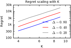
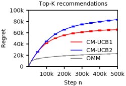
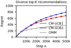
(a)                                     (b)                                        (c)

Figure 1: a. The $n$-step regret of ${\tt I\mathchar 45\relax UCB1}$ in the synthetic problem in Section 5.1 as a function of $K$. b. The regret of ${\tt I\mathchar 45\relax UCB1}$, ${\tt I\mathchar 45\relax UCB2}$, and ${\tt OMM}$ in the top-$K$ recommendation problem in Section 5.2. c. The regret of ${\tt I\mathchar 45\relax UCB1}$, ${\tt I\mathchar 45\relax UCB2}$, and ${\tt OMM}$ in the diverse top-$K$ recommendation problem in Section 5.2.

5.1 Regret Scaling

The first experiment shows that the regret of ${\tt I\mathchar 45\relax UCB1}$ grows as suggested by our gap-dependent upper bound in Theorem 2. We experiment with uniform matroids of rank $K$ where the ground set is $E=[K^{2}]$. The $i$-th entry of $\bm{w}_{t}$, $\bm{w}_{t}(i)$, is an independent Bernoulli variable with mean $\bar{w}(i)=0.5(1-\Delta\mathbbm{1}\!\left(i>K\right))$ for $\Delta\in(0,1)$. The baseline set is the last $K$ items in $E$, $B_{0}=[K^{2}]\setminus[K(K-1)]$. The key property of our class of problems is that the regret of any item in $B_{0}$ is the same as that of any suboptimal item, and therefore the regret of ${\tt I\mathchar 45\relax UCB1}$ should be dominated by the gap-dependent term in Theorem 2. This term is $O(K^{3})$ because $L=K^{2}$. We vary $K$ and report the $n$-step regret in $100\text{k}$ steps for multiple values of $\Delta$.

Fig. 1a shows log-log plots of the regret of ${\tt I\mathchar 45\relax UCB1}$ as a function of $K$ for three values of $\Delta$. The slopes of the plots are $2.99$ ($\Delta=0.8$), $2.98$ ($\Delta=0.4$), and $2.99$ ($\Delta=0.2$). This means that the regret is cubic in $K$, as suggested by our upper bound.

5.2 Recommender System Experiment

In the second experiment, we apply ${\tt I\mathchar 45\relax UCB}$ to the two recommendation problems discussed in Section 2.3. In each problem, we recommend $K$ most attractive movies out of $L$ subject to a different matroid constraint. We experiment with the MovieLens dataset from February 2003 [21], where $6$ thousand users give one million ratings to $4$ thousand movies.

Our learning problems are formulated as follows. The set $E$ are $200$ movies from the MovieLens dataset. The set is partitioned as $E=\bigcup_{i=1}^{10}E_{i}$, where $E_{i}$ are $20$ most popular movies in the $i$-th most popular MovieLens movie genre that are not in $E_{1},\dots,E_{i-1}$. The weight of item $e$ at time $t$, $\bm{w}_{t}(e)$, indicates that item $e$ attracts the user at time $t$. We assume that $\bm{w}_{t}(e)=1$ if and only if the user rated item $e$ in our dataset. This indicates that the user watched movie $e$ at some point in time, perhaps because the movie was attractive. The user at time $t$ is drawn randomly from all MovieLens users. The goal of the learning agent is to learn a list of items with the highest expected number of attractive movies on average, subject to a constraint.

We experiment with two constraints. The first problem is a uniform matroid of rank $K=10$. The optimal solution is the set of $K$ most attractive movies. This setting is also known as top-$K$ recommendations. The baseline set $B_{0}$ are the $11$-th to $20$-th most attractive movies. The second problem is a partition matroid of rank $K=10$, where the partition is $\{E_{i}\}_{i=1}^{10}$. The optimal solution are most attractive movies in each $E_{i}$. This setting can be viewed as diverse top-$K$ recommendations. The baseline set $B_{0}$ are second most attractive movies in each $E_{i}$.

Our results are reported in Figures 1b and 1c. We observe several trends. First, the regret of all algorithms flattens over time, which shows that they learn near-optimal solutions. Second, the regret of ${\tt I\mathchar 45\relax UCB2}$ is higher than that of ${\tt I\mathchar 45\relax UCB1}$. This is because ${\tt I\mathchar 45\relax UCB2}$ is a variant of ${\tt I\mathchar 45\relax UCB1}$ that does not know the values of suboptimal items, and therefore needs to estimate them. Both of our algorithms satisfy our conservative constraint in (1) at each time $t$. Third, we observe that ${\tt OMM}$ achieves the lowest regret. But it also violates our conservative constraints. In Figures 1b and 1c, the numbers of violated constraints are more than $16$ and $158$ thousand, respectively. In the latter problem, this is one violated constraint in every three actions on average. Finally, note that the regret of ${\tt I\mathchar 45\relax UCB}1$ and ${\tt I\mathchar 45\relax UCB}2$ is less than $(K-1)$ times ($K=10$) the regret of ${\tt OMM}$, as predicted by our regret bounds.

6 Related Work

Online learning with matroids was introduced by Kveton et al. [18], and also studied by Talebi and Proutiere [27]. However, they do not consider any notion of conservatism. Our ${\tt I\mathchar 45\relax UCB}$ algorithm borrows ideas and the MaxBasis method from their algorithm.

Conservatism in online learning was introduced by Wu et al. [29]. They consider the standard multi-armed bandit problem with no structural assumption about their actions. Their constraint is cumulative, and this allows the learner to take bad actions once in a while, but our instantaneous constraint (1) explicitly forbids this by design. However, note that our setting and algorithm applies to combinatorial action spaces, and hence is less general.

Kazerouni et al. [17] study conservatism in linear bandits. Their constraint is also cumulative; furthermore the time complexity of their algorithm grows with time when the rewards of the basline policy are unknown. ${\tt I\mathchar 45\relax UCB}$ is efficient because it exploits the matroid structure of the action space.

Bastani et al. [4] study contextual bandits and propose diversity assumptions on the environment. Intuitively, if contexts vary a lot over time, the environment explores on your behalf and you need not explore. In our setting, the learner actively explores, albeit in a constrained fashion.

Radlinski and Joachims [23] propose randomizing the order of presented items to estimate their true relevance in the presence of item and position biases. While their algorithm guarantees that the quality of the presented items is unaffected, it does not learn a better policy. The idea of interleaving has been used to evaluate information retrieval systems and Chapelle et al. [8] validate its efficacy, but they too do not learn a better policy. Our algorithm learns a better policy, as seen in our regret plots. While we do not consider item and position biases in this work, we hope to do so in the future work.

7 Conclusions

In this paper, we study controlled exploration in combinatorial action spaces using interleaving, and precisely formulate the learning problem in the action space of matroids. Our conservate formulation is more suitable for combinatorial spaces than existing notions of conservatism. We propose an algorithm for solving our problem, ${\tt I\mathchar 45\relax UCB}$, and prove gap-dependent upper bounds on its regret. ${\tt I\mathchar 45\relax UCB}$ exploits the idea of interleaving, and hence can evaluate an action without ever taking that action.

We leave open several questions of interest. First, we only study the case of $\alpha=1/K$. Our algorithm generalizes to higher values of $\alpha$ in uniform and partition matroids, because they satisfy the property that $\forall\,B_{1},B_{2}\in\mathcal{B}$, there exists a bijection $\sigma_{B_{1},B_{2}}:B_{1}\to B_{2}$ such that $(B_{1}\setminus X)\cup\sigma_{B_{1},B_{2}}(X)\in\mathcal{B}$ $\forall X\subseteq B_{1}$. Matroids that satisfy this property are called strongly base-orderable, and one can generalize ${\tt I\mathchar 45\relax UCB}$ and its analysis to these matroids for higher values of $\alpha$ (see Section 4.3). It is not clear how to extend our results beyond $\alpha=1/K$ when the matroid is not strongly base-orderable.

Second, we exploit the modularity of our reward function. In general, it may not be possible to build unbiased estimators with interleaving. For e.g., clicks are known to be position-biased, and click models that take this into account have non-linear reward functions [10]. But it may be possible to build biased estimators with the right bias, such that a more attractive item never appears to be less attractive than a less attractive item [30].

Third, Lemma 1 only guarantees the existence of a bijection, but it is not constructive. The construction is straightforward for uniform and partition matroids in our experiments. Fourth, we also leave open the question of a lower bound. Finally, note that our new analysis based on Lemma 1 significantly simplifies the original analysis of OMM in Kveton et al. [18].

Appendix A Appendix

We define a “good” event

$$\mathcal{E}_{t}=\{\forall\,e\in E:|\bar{w}(e)-\hat{\bm{w}}_{\bm{T}_{t-1}(e)}(e)|\leq c_{n,\bm{T}_{t-1}(e)}\}\,,$$ (8)

which states that $\bar{w}(e)$ is inside the high-probability confidence interval around $\hat{\bm{w}}_{\bm{T}_{t-1}(e)}(e)$ for all items $e$ at the beginning of time $t$.

Lemma 2.

Let $\mathcal{E}_{r}$ be the good event in (8). Then

$$\mathbb{P}\left(\bigcup_{r=1}^{n/K}\bar{\mathcal{E}}_{r}\right)\leq\sum_{r=1}^{n/K}\mathbb{E}\!\left[\mathbbm{1}\!\left(\bar{\mathcal{E}}_{r}\right)\right]\leq\frac{2L}{Kn}\,.$$

Proof.

From the definition of our confidence intervals and Hoeffding’s inequality [5],

$$\mathbb{P}({|\bar{w}(e)-\hat{\bm{w}}_{s}(e)|\geq c_{t,s}})\leq 2\exp[-3\log t]$$

for any $e\in E$, $s\in[n]$, and $t\in[n]$. Therefore,

$$\mathbb{P}\left(\bigcup_{r=1}^{n/K}\bar{\mathcal{E}}_{r}\right) \leq\sum_{r=1}^{n/K}\mathbb{P}(\bar{\mathcal{E}}_{r})$$

$$\leq\sum_{r=1}^{n/K}\sum_{e\in E}\sum_{s=1}^{rK}\mathbb{P}(|\bar{w}(e)-\hat{\bm{w}}_{s}(e)|\geq c_{n,s})$$

$$\leq 2\sum_{e\in E}\frac{1}{Kn}\,.$$

This concludes our proof. ∎

Lemma 3.

Let $A$ be the maximum weight basis with respect to weights $w$. Let $B$ be any basis and let $\rho:A\to B$ be the bijection in Lemma 1. Then

$$\forall a\in A:w(a)\geq w(\rho(a))\,.$$

Proof.

Fix $a\in A$ and let $b=\rho(a)$. By Lemma 1, $A^{a}_{b}=A\setminus\{a\}\cup\{b\}\in\mathcal{B}$. Now note that $A$ is the maximum weight basis with respect to $w$. Therefore,

$$w(a)-w(b)=\sum_{e\in A}w(e)-\sum_{e\in A^{a}_{b}}w(e)\geq 0\,.$$

This concludes our proof. ∎

See 1

Proof.

At time $t$, the baseline set $\bm{B}_{t}$ is the maximum weight basis with respect to $\bm{v}_{t}$. Therefore, by Lemma 3, there exists a bijection $\bm{\rho}:\bm{B}_{t}\rightarrow B_{0}$ such that

$$\forall b\in\bm{B}_{t}:\bm{v}_{t}(b)\geq\bm{v}_{t}(\bm{\rho}(b))\,.$$

From the definition of $\bm{v}_{t}$, $\bm{v}_{t}(\bm{\rho}(b))=\bar{w}(\bm{\rho}(b))$ for any $b\in\bm{B}_{t}$, and thus

$$\forall b\in\bm{B}_{t}:\bm{v}_{t}(b)\geq\bar{w}(\bm{\rho}(b))\,.$$

Now suppose that event $\mathcal{E}_{t}$ in (8) happens. Then $\bar{w}(e)\geq\bm{L}_{t}(e)$ for any $e\in E$, and it follows that

$$\forall b\in\bm{B}_{t}:\bar{w}(b)\geq\bar{w}(\bm{\rho}(b))\,.$$

Since any action at time $t$ contains $K-1$ items from $\bm{B}_{t}$, the constraint in (1) is satisfied when event $\mathcal{E}_{t}$ happens.

Finally, we prove that $\mathbb{P}(\cup_{t}\bar{\mathcal{E}}_{t})\leq 2L/(Kn)$ in Lemma 2. Therefore, $\mathbb{P}(\mathcal{E}_{t})\geq\mathbb{P}(\cap_{t}\mathcal{E}_{t})\geq 1-2L/(Kn)$. This concludes our proof. ∎

Lemma 4.

For any $e,e^{\ast}$, if $e\in\bm{D}_{t}$ and $e=\bm{\pi}_{t}(e^{\ast})$, we have that

$$2c_{n,\bm{T}_{t-1}(e)}\geq\bar{w}(e^{\ast})-\bar{w}(e),\qquad\text{and}\qquad\bm{T}_{t-1}(e)\leq\frac{6\log n}{\Delta_{e,e^{\ast}}^{2}}\leq\frac{6\log n}{\Delta_{e,\min}^{2}},$$ (9)

where $\Delta_{e,\min}$ is defined in (5).

Proof.

Since the decision set $\bm{D}_{t}$ is chosen using upper confidence bounds, we have that $\bm{U}_{t}(e)\geq\bm{U}_{t}(e^{\ast})$. This gives us:

$$\bar{w}(e)+2c_{n,\bm{T}_{t-1}(e)}\geq\hat{\bm{w}}_{t-1}(e)+c_{n,\bm{T}_{t-1}(e)}=\bm{U}_{t}(e)\geq\bm{U}_{t}(e^{\ast})\geq\bar{w}(e^{\ast}).$$

This implies the first inequality in (9). Substituting the expression for $c_{n,\bm{T}_{t-1}(e)}$ from (4) yields the bound on $\bm{T}_{t-1}(e)$ in (9). ∎

Lemma 5.

For any $e^{\ast}\in A^{\ast}$, $e\in\bm{D}_{t}$, and $e^{\prime}\in\bm{B}_{t}$ such that $e=\bm{\pi}_{t}(e^{\ast})$ and $e^{\prime}=\bm{\sigma}_{t}(e)$,

• If $e\in A^{\ast}$, then $e=e^{\ast}$ and

  $$2c_{n,\bm{T}_{t-1}(e^{\ast})}\geq\bar{w}(e^{\ast})-\bar{w}(e^{\prime}),\qquad\text{and}\qquad\bm{T}_{t-1}(e^{\ast})\leq\frac{6\log n}{\Delta_{e^{\prime},e^{\ast}}^{2}}\leq\frac{6\log n}{\Delta_{e^{\ast},\min}^{{}^{\ast}2}},$$ (10)

  where $\Delta^{\ast}_{e^{\ast},\min}$ is defined in (6).

• If $e\notin A^{\ast}$,

  $$4c_{n,\bm{T}_{t-1}(e)}\geq\bar{w}(e^{\ast})-\bar{w}(e^{\prime}).$$ (11)

Proof.

Since the baseline set is selected using lower confidence bounds, we have that $\bm{L}_{t}(e^{\prime})\geq\bm{L}_{t}(e)$. This gives us:

$$\bar{w}(e^{\prime})\geq\bm{L}_{t}(e^{\prime})\geq\bm{L}_{t}(e)\geq\bar{w}(e)-2c_{n,\bm{T}_{t-1}(e)}$$

This implies that

$$2c_{n,\bm{T}_{t-1}(e)}\geq\bar{w}(e)-\bar{w}(e^{\prime}).$$ (12)

• If $e\in A^{\ast}$, then since $e=\bm{\pi}_{t}(e^{\ast})$, we must have that $e\neq e^{\ast}$. Assume otherwise. Then $A^{\ast}\setminus\{e^{\ast}\}\cup\{e\}$ is a basis (by Lemma 1) of size $(K-1)$, which contradicts the fact that all bases have the same cardinality $K$. Substituting $e=e^{\ast}$ in (12) gives the first inequality in (10). The $\bm{T}_{t-1}(e^{\ast})$ bound in (10) follows by substituting the expression of $c_{n,\bm{T}_{t-1}(e)}$ from (4).

• If $e\notin A^{\ast}$, note that the confidence interval inequality in (9) from Lemma 4 still holds because $e\in\bm{D}_{t}$. (11) then follows by adding this and (12).

∎

See 2

Proof.

We first decompose the regret depending on whether the event $\bar{\mathcal{E}}=\bigcup\limits_{t=1}^{n/K}\bar{\mathcal{E}}_{t}$ happens or not, where $\mathcal{E}_{t}$ is defined in (8).

Let $\bm{R}_{t}$ denote the regret at time $t$. Then, we can decompose the regret of ${\tt I\mathchar 45\relax UCB}1$ as:

$$R(n) =\mathbb{E}\!\left[\mathbbm{1}\!\left(\bar{\mathcal{E}}\right)\sum\limits_{t=1}^{n/K}\bm{R}_{t}\right]+\mathbb{E}\!\left[\mathbbm{1}\!\left(\mathcal{E}\right)\sum\limits_{t=1}^{n/K}\mathbbm{1}\!\left(\bm{R}_{t}\right)\right]$$ (13)

Let us first analyze the case when $\bar{\mathcal{E}}$ holds. The probability of this event by Lemma 2 is $\frac{2L}{Kn}$. Since the maximum regret in $n$ steps can be $Kn$, the contribution of the first term is $2L$.

We assume $\mathcal{E}$ holds in the remaining proof. The expected regret at time $t$ can be written as

$$\mathbb{E}\!\left[R_{t}\right] =K\sum_{e^{\ast}\in A^{\ast}}\bar{w}(e^{\ast})-(K-1)\sum_{e^{\prime}\in\bm{B}_{t}}\bar{w}(e^{\prime})-\sum_{e\in\bm{D}_{t}}\bar{w}(e)$$

$$=\left(\sum_{e^{\ast}\in A^{\ast}}\bar{w}(e^{\ast})-\sum_{e\in\bm{D}_{t}}\bar{w}(e)\right)+(K-1)\left(\sum_{e^{\ast}\in A^{\ast}}\bar{w}(e^{\ast})-\sum_{e^{\prime}\in\bm{B}_{t}}\bar{w}(e^{\prime})\right).$$ (14)

Let us first bound the regret due to the first term. When we sum the first term in (14) over all times $t$, we get

$$\sum_{t=1}^{n/K}\left(\sum_{e^{\ast}\in A^{\ast}}\bar{w}(e^{\ast})-\sum_{e\in\bm{D}_{t}}\bar{w}(e)\right) \overset{(a)}{\leq}\sum_{t=1}^{n/K}\sum_{e\in\bm{D}_{t}}2c_{n,\bm{T}_{t-1}(e)}\leq\sum_{e\in E\setminus A^{\ast}}\sum_{t=1}^{n/K}2\sqrt{\frac{1.5\log n}{\bm{T}_{t-1}(e)}}\mathbbm{1}\!\left(e\in\bm{D}_{t}\right)$$

where $(a)$ follows from the first inequality in (9) in Lemma 4. Since a) the counter $\bm{T}_{t-1}(e)$ increments every time $e$ is played, b) second inequality in Eq. (9) holds by Lemma 4, and

$$\sum_{s=1}^{m}\frac{1}{\sqrt{s}}\leq 1+2\sqrt{m},$$ (15)

we can bound the regret due to the first term as

$$\sum_{t=1}^{n/K}\left(\sum_{e^{\ast}\in A^{\ast}}\bar{w}(e^{\ast})-\sum_{e\in\bm{D}_{t}}\bar{w}(e)\right) \leq\sum_{e\in E\setminus A^{\ast}}2\sqrt{1.5\log n}\left(1+2\sqrt{\frac{6\log n}{\Delta_{e,\min}^{2}}}\right)$$

$$\leq 12\sum_{e\in E\setminus A^{\ast}}\frac{1}{\Delta_{e,\min}}\log n+L\sqrt{6\log n}$$ (16)

Let us now bound the regret due to the second term in (14). When we sum the second term in (14) over all times $t$, we get

$$(K-1)\sum_{t=1}^{n/K}\left(\sum_{e^{\ast}\in A^{\ast}}\bar{w}(e^{\ast})-\sum_{e^{\prime}\in\bm{B}_{t}}\bar{w}(e^{\prime})\right)$$

$$\overset{(a)}{\leq}\, (K-1)\left(\sum_{t=1}^{n/K}\sum_{e\in\bm{D}_{t}\cap A^{\ast}}2c_{n,\bm{T}_{t-1}(e)}+\sum_{t=1}^{n/K}\sum_{e\in\bm{D}_{t}\setminus A^{\ast}}4c_{n,\bm{T}_{t-1}(e)}\right)$$

$$=\, (K-1)\left(\sum_{e\in A^{\ast}}\sum_{t=1}^{n/K}2\sqrt{\frac{1.5\log n}{\bm{T}_{t-1}(e)}}\mathbbm{1}\!\left(e\in\bm{D}_{t}\right)+\sum_{e\in E\setminus A^{\ast}}\sum_{t=1}^{n/K}4\sqrt{\frac{1.5\log n}{\bm{T}_{t-1}(e)}}\mathbbm{1}\!\left(e\in\bm{D}_{t}\right)\right)$$ (17)

where $(a)$ follows from (10) and (11) in Lemma 5. We use the $\bm{T}_{t-1}(e^{\ast})$ bound in (10) to bound the first term, and the $\bm{T}_{t-1}(e)$ bound in (9) to bound the second term in (17). Then, from the fact that the counter $\bm{T}_{t-1}(e)$ is incremented every time $e$ is chosen, and (15), we can bound the regret due to the second term in (14) as

$$(K-1)\sum_{t=1}^{n/K}\left(\sum_{e^{\ast}\in A^{\ast}}\bar{w}(e^{\ast})-\sum_{e^{\prime}\in\bm{B}_{t}}\bar{w}(e^{\prime})\right)$$

$$\leq\, (K-1)\left(\sum_{e^{\ast}\in A^{\ast}}2\sqrt{1.5\log n}\left(1+2\sqrt{\frac{6\log n}{\Delta_{e^{\ast},\min}^{{}^{\prime}2}}}\right)+\sum_{e\in E\setminus A^{\ast}}4\sqrt{1.5\log n}\left(1+2\sqrt{\frac{6\log n}{\Delta_{e,\min}^{2}}}\right)\right)$$

$$\leq\, 24(K-1)\sum_{e\in E\setminus A^{\ast}}\frac{1}{\Delta_{e,\min}}\log n+12(K-1)\sum_{e^{\ast}\in A^{\ast}}\frac{1}{\Delta^{\ast}_{e^{\ast},\min}}\log n$$

$$\qquad+L(K-1)\sqrt{24\log n}+K(K-1)\sqrt{6\log n}$$ (18)

Adding (16), (18), and the contribution from the failure event $\bar{\mathcal{E}}$ yields the upper bound in the theorem statement. ∎

See 3

Proof.

At time $t$, the baseline set $\bm{B}_{t}$ is the maximum weight basis with respect to $\bm{v}_{t}$. Therefore, by Lemma 3, there exists a bijection $\bm{\rho}:\bm{B}_{t}\rightarrow B_{0}$ such that

$$\forall b\in\bm{B}_{t}:\bm{v}_{t}(b)\geq\bm{v}_{t}(\bm{\rho}(b))\,.$$

Now we consider two cases. First, suppose that $b\in B_{0}$. Then by Lemma 3, $b=\bm{\rho}(b)$, and $\bar{w}(b)\geq\bar{w}(\bm{\rho}(b))$ from our assumption. Second, suppose that $b\notin B_{0}$. Then from $\bm{v}_{t}(b)=\bm{L}_{t}(b)$ and $\bm{v}_{t}(\bm{\rho}(b))=\bm{U}_{t}(\bm{\rho}(b))$, and

$$\bar{w}(b)\geq\bm{L}_{t}(b)\geq\bm{U}_{t}(\bm{\rho}(b))\geq\bar{w}(\bm{\rho}(b))$$

under event $\mathcal{E}_{t}$. Since any action at time $t$ contains $K-1$ items from $\bm{B}_{t}$, the constraint in (1) is satisfied when event $\mathcal{E}_{t}$ happens.

Finally, we prove that $\mathbb{P}(\cup_{t}\bar{\mathcal{E}}_{t})\leq 2L/(Kn)$ in Lemma 2. Therefore, $\mathbb{P}(\mathcal{E}_{t})\geq\mathbb{P}(\cap_{t}\mathcal{E}_{t})\geq 1-2L/(Kn)$. This concludes our proof. ∎

Lemma 6.

For any $e^{\ast}\in A^{\ast}$, $e\in\bm{D}_{t}$, and $e^{\prime}\in\bm{B}_{t}$ such that $e^{\prime}\in B_{0}$, $e=\bm{\pi}_{t}(e^{\ast})$, and $e^{\prime}=\bm{\sigma}_{t}(e)$,

• If $e\in A^{\ast}$, and $c_{n,\bm{T}_{t-1}(e^{\prime})}\leq c_{n,\bm{T}_{t-1}(e)}$, then $e=e^{\ast}$, and

  $$4c_{n,\bm{T}_{t-1}(e^{\ast})}\geq\bar{w}(e^{\ast})-\bar{w}(e^{\prime}),\qquad\text{and}\qquad\bm{T}_{t-1}(e^{\ast})\leq\frac{24\log n}{\Delta_{e^{\prime},e^{\ast}}^{2}}.$$ (19)

• If $e\in\bm{D}_{t}\setminus A^{\ast}$ and $c_{n,\bm{T}_{t-1}(e^{\prime})}\leq c_{n,\bm{T}_{t-1}(e)}$, then

  $$6c_{n,\bm{T}_{t-1}(e)}\geq\bar{w}(e^{\ast})-\bar{w}(e^{\prime}).$$ (20)

• If $c_{n,\bm{T}_{t-1}(e^{\prime})}>c_{n,\bm{T}_{t-1}(e)}$, then

  $$4c_{n,\bm{T}_{t-1}(e^{\prime})}\geq\bar{w}(e)-\bar{w}(e^{\prime}),\qquad\text{and}\qquad\bm{T}_{t-1}(e^{\prime})\leq\frac{24\log n}{\Delta_{e^{\prime},e}^{2}}\leq\frac{24\log n}{\Delta_{e^{\prime},\min}^{{}^{\prime}2}},$$ (21)

  where $\Delta^{\prime}_{e^{\prime},\min}$ is defined in (7).

Proof.

For items $e^{\prime}\in B_{0}\cap\bm{B}_{t}$, we have that $\bm{U}_{t}(e^{\prime})\geq\bm{L}_{t}(e)$. This gives us

$$\bar{w}(e^{\prime})+2c_{n,\bm{T}_{t-1}(e^{\prime})}\geq\bm{U}_{t}(e^{\prime})\geq\bm{L}_{t}(e)\geq\bar{w}(e)-2c_{n,\bm{T}_{t-1}(e)}$$

This implies that

$$2c_{n,\bm{T}_{t-1}(e)}+2c_{n,\bm{T}_{t-1}(e^{\prime})}\geq\bar{w}(e)-\bar{w}(e^{\prime}).$$ (22)

• If $e\in A^{\ast}$, then $e=e^{\ast}$ by the same argument as in the proof of Lemma 5(a). Substituting $e=e^{\ast}$ in (22) gives the first inequality in (19). Substituting the expression for $c_{n,\bm{T}_{t-1}(e^{\ast})}$ from (4) gives the second inequality in (19).

• If $e\in\bm{D}_{t}\setminus A^{\ast}$ and $c_{n,\bm{T}_{t-1}(e^{\prime})}\leq c_{n,\bm{T}_{t-1}(e)}$, adding the confidence interval inequalities in (22) and (9) gives (20).

• We assume $\bar{w}(e)>\bar{w}(e^{\prime})$, because otherwise the regret contribution is bounded by $0$. Then, $c_{n,\bm{T}_{t-1}(e^{\prime})}>c_{n,\bm{T}_{t-1}(e)}$ and (22) imply the first inequality in (21). Substituting the expression for $c_{n,\bm{T}_{t-1}(e^{\prime})}$ from (4) gives the bound on $\bm{T}_{t-1}(e^{\prime})$ in (21).

∎

Corollary 1.

For any $e^{\ast}\in A^{\ast}\cap\bm{D}_{t}$, and $e^{\prime}\in\bm{B}_{t}$ such that and $e^{\prime}=\bm{\sigma}_{t}(e^{\ast})$, if a) $e^{\prime}\notin B_{0}$, or b) $e^{\prime}\in B_{0}$ and $c_{n,\bm{T}_{t-1}(e^{\prime})}\leq c_{n,\bm{T}_{t-1}(e^{\ast})}$, we have

$$\bm{T}_{t-1}(e^{\ast})\leq\frac{24\log n}{\Delta_{e^{\ast},\min}^{\ast 2}},$$ (23)

where $\Delta^{\ast}_{e^{\ast},\min}$ is defined in (6).

Proof.

The proof follows by taking the maximum of the upper bounds in (10) and (19) over all $e^{\prime}$ that satisfy the conditions of Lemma 5(a) or Lemma 6(a). ∎

See 4

Proof.

Similar to the proof of ${\tt I\mathchar 45\relax UCB}1$, we use (13) to break down the regret depending on whether the failure event $\bar{\mathcal{E}}=\bigcup\limits_{t=1}^{n/K}\bar{\mathcal{E}}_{t}$ holds or not. The contribution from the event $\bar{\mathcal{E}}$ is again bounded by $2L$.

We assume $\mathcal{E}$ holds in the remaining proof. We again use (14) to decompose the regret, and the bound on the first term from (16) holds.

The difference in ${\tt I\mathchar 45\relax UCB}2$ compared to ${\tt I\mathchar 45\relax UCB}1$ is that while selecting the baseline set $\bm{B}_{t}$ in ${\tt I\mathchar 45\relax UCB}2$, we use upper confidence intervals for items in $B_{0}$.

We now sum the second term in (14) over all times $t$,

$$(K-1)\sum_{t=1}^{n/K}\left(\sum_{e^{\ast}\in A^{\ast}}\bar{w}(e^{\ast})-\sum_{e^{\prime}\in\bm{B}_{t}}\bar{w}(e^{\prime})\right)$$

$$= (K-1)\sum_{t=1}^{n/K}\left(\left(\sum_{\stackrel{{\scriptstyle e^{\ast}\in A^{\ast},}}{{\bm{\sigma}_{t}(\bm{\pi}_{t}(e^{\ast}))\notin B_{0}}}}\bar{w}(e^{\ast})-\sum_{e^{\prime}\in\bm{B}_{t}\setminus B_{0}}\bar{w}(e^{\prime})\right)+\left(\sum_{\stackrel{{\scriptstyle e^{\ast}\in A^{\ast},}}{{\bm{\sigma}_{t}(\bm{\pi}_{t}(e^{\ast}))\in B_{0}}}}\bar{w}(e^{\ast})-\sum_{e^{\prime}\in\bm{B}_{t}\cap B_{0}}\bar{w}(e^{\prime})\right)\right)$$

$$\leq (K-1)\sum_{t=1}^{n/K}\left(\left(\sum_{\stackrel{{\scriptstyle e\in\bm{D}_{t}\cap A^{\ast},}}{{\bm{\pi}_{t}(e)\notin B_{0}}}}2c_{n,\bm{T}_{t-1}(e)}+\sum_{\stackrel{{\scriptstyle e\in\bm{D}_{t}\setminus A^{\ast},}}{{\bm{\pi}_{t}(e)\notin B_{0}}}}4c_{n,\bm{T}_{t-1}(e)}\right)\right.$$

$$+ \left.\left(\sum_{\stackrel{{\scriptstyle e\in A^{\ast}\cap\bm{D}_{t},\bm{\pi}_{t}(e)=e^{\prime}\in B_{0}}}{{c_{n,\bm{T}_{t-1}(e)}>c_{n,\bm{T}_{t-1}(e^{\prime})}}}}4c_{n,\bm{T}_{t-1}(e)}+\sum_{\stackrel{{\scriptstyle e\in\bm{D}_{t}\setminus A^{\ast},\bm{\pi}_{t}(e)=e^{\prime}\in B_{0}}}{{c_{n,\bm{T}_{t-1}(e)}>c_{n,\bm{T}_{t-1}(e^{\prime})}}}}6c_{n,\bm{T}_{t-1}(e)}+\sum_{\stackrel{{\scriptstyle e\in\bm{D}_{t},\bm{\pi}_{t}(e)=e^{\prime}\in B_{0}}}{{c_{n,\bm{T}_{t-1}(e)}>c_{n,\bm{T}_{t-1}(e^{\prime})}}}}4c_{n,\bm{T}_{t-1}(e^{\prime})}\right)\right)$$

$$\leq (K-1)\left(\sum_{e^{\ast}\in A^{\ast}}\sum_{t=1}^{n/K}4c_{n,\bm{T}_{t-1}(e^{\ast})}\mathbbm{1}\!\left(e^{\ast}\in\bm{D}_{t}\right)+\sum_{e\in E\setminus A^{\ast}}\sum_{t=1}^{n/K}6c_{n,\bm{T}_{t-1}(e)}\mathbbm{1}\!\left(e\in\bm{D}_{t}\right)\right.$$

$$\left.+\sum_{e^{\prime}\in B_{0}}\sum_{t=1}^{n/K}4c_{n,\bm{T}_{t-1}(e^{\prime})}\mathbbm{1}\!\left(e^{\prime}\in\bm{B}_{t}\right)\right)$$

Similar to the proof of ${\tt I\mathchar 45\relax UCB}1$, we substitute for the confidence intervals using (4). We then bound the first term using (23), second term using (9), and third term using (21).

$$(K-1) \sum_{t=1}^{n/K}\left(\sum_{e^{\ast}\in A^{\ast}}\bar{w}(e^{\ast})-\sum_{e^{\prime}\in\bm{B}_{t}}\bar{w}(e^{\prime})\right)$$

$$\leq(K-1) \left(\sum_{e^{\ast}\in A^{\ast}}\frac{48\log n}{\Delta^{\ast}_{e^{\ast},\min}}+\sum_{e\in E\setminus A^{\ast}\setminus B_{0}}\frac{36\log n}{\Delta_{e,\min}}+\sum_{e^{\prime}\in B_{0}}\frac{48\log n}{\Delta^{\prime}_{e^{\prime},\min}}\right)$$

$$+(K-1) \left(K\sqrt{24\log n}+L\sqrt{48\log n}+K\sqrt{24\log n}\right)$$ (24)

Adding (16), (24) and the contribution from the failure event $\bar{\mathcal{E}}$ yields the upper bound in the theorem statement. ∎

References

- Adomavicius and Tuzhilin [2015] Gediminas Adomavicius and Alexander Tuzhilin. Context-aware recommender systems. In Recommender systems handbook, pages 191–226. Springer, 2015.
- Audibert et al. [2013] Jean-Yves Audibert, Sébastien Bubeck, and Gábor Lugosi. Regret in online combinatorial optimization. Mathematics of Operations Research, 39(1):31–45, 2013.
- Auer et al. [2002] Peter Auer, Nicolo Cesa-Bianchi, and Paul Fischer. Finite-time analysis of the multiarmed bandit problem. Machine learning, 47(2-3):235–256, 2002.
- Bastani et al. [2017] Hamsa Bastani, Mohsen Bayati, and Khashayar Khosravi. Exploiting the natural exploration in contextual bandits. arXiv preprint arXiv:1704.09011, 2017.
- Boucheron et al. [2013] Stéphane Boucheron, Gábor Lugosi, and Pascal Massart. Concentration inequalities: A nonasymptotic theory of independence. Oxford university press, 2013.
- Broder [2008] Andrei Z Broder. Computational advertising and recommender systems. In Proceedings of the 2008 ACM conference on Recommender systems, pages 1–2. ACM, 2008.
- Brualdi [1969] Richard A Brualdi. Comments on bases in dependence structures. Bulletin of the Australian Mathematical Society, 1(2):161–167, 1969.
- Chapelle et al. [2012] Olivier Chapelle, Thorsten Joachims, Filip Radlinski, and Yisong Yue. Large-scale validation and analysis of interleaved search evaluation. ACM Transactions on Information Systems (TOIS), 30(1):6, 2012.
- Chen et al. [2013] Wei Chen, Yajun Wang, and Yang Yuan. Combinatorial multi-armed bandit: General framework and applications. In International Conference on Machine Learning, pages 151–159, 2013.
- Chuklin et al. [2015] Aleksandr Chuklin, Ilya Markov, and Maarten de Rijke. Click models for web search. Synthesis Lectures on Information Concepts, Retrieval, and Services, 7(3):1–115, 2015.
- Cremonesi et al. [2011] Paolo Cremonesi, Franca Garzotto, Sara Negro, Alessandro Vittorio Papadopoulos, and Roberto Turrin. Looking for “good” recommendations: A comparative evaluation of recommender systems. In IFIP Conference on Human-Computer Interaction, pages 152–168. Springer, 2011.
- Deshpande and Karypis [2004] Mukund Deshpande and George Karypis. Item-based top-n recommendation algorithms. ACM Transactions on Information Systems (TOIS), 22(1):143–177, 2004.
- Edmonds [1971] Jack Edmonds. Matroids and the greedy algorithm. Mathematical programming, 1(1):127–136, 1971.
- Gai et al. [2012] Yi Gai, Bhaskar Krishnamachari, and Rahul Jain. Combinatorial network optimization with unknown variables: Multi-armed bandits with linear rewards and individual observations. IEEE/ACM Transactions on Networking (TON), 20(5):1466–1478, 2012.
- Garivier and Cappé [2011] Aurélien Garivier and Olivier Cappé. The kl-ucb algorithm for bounded stochastic bandits and beyond. In Proceedings of the 24th annual Conference On Learning Theory, pages 359–376, 2011.
- Kalyanakrishnan et al. [2012] Shivaram Kalyanakrishnan, Ambuj Tewari, Peter Auer, and Peter Stone. Pac subset selection in stochastic multi-armed bandits. In ICML, volume 12, pages 655–662, 2012.
- Kazerouni et al. [2017] Abbas Kazerouni, Mohammad Ghavamzadeh, Yasin Abbasi, and Benjamin Van Roy. Conservative contextual linear bandits. In Advances in Neural Information Processing Systems, pages 3913–3922, 2017.
- Kveton et al. [2014a] Branislav Kveton, Zheng Wen, Azin Ashkan, Hoda Eydgahi, and Brian Eriksson. Matroid bandits: Fast combinatorial optimization with learning. arXiv preprint arXiv:1403.5045, 2014a.
- Kveton et al. [2014b] Branislav Kveton, Zheng Wen, Azin Ashkan, and Michal Valko. Learning to act greedily: Polymatroid semi-bandits. arXiv preprint arXiv:1405.7752, 2014b.
- Kveton et al. [2015] Branislav Kveton, Zheng Wen, Azin Ashkan, and Csaba Szepesvari. Tight regret bounds for stochastic combinatorial semi-bandits. In Artificial Intelligence and Statistics, pages 535–543, 2015.
- Lam and Herlocker [2016] Shyong Lam and Jon Herlocker. MovieLens Dataset. http://grouplens.org/datasets/movielens/, 2016.
- Oxley [2006] James G Oxley. Matroid theory, volume 3. Oxford University Press, USA, 2006.