Dynamical off-equilibrium scaling across magnetic
first-order phase transitions

Stefano Scopa^a, and Sascha Wald^b,

^a Laboratoire de Physique et Chimie Théoriques, UMR CNRS 7019, Université de Lorraine BP 70239, F-54506 Vandoeuvre-lès-Nancy Cedex, France

^b SISSA - International School for Advanced Studies and INFN,

via Bonomea 265, I–34136 Trieste, Italy

We investigate the off-equilibrium dynamics of a classical spin system with $O(n)$ symmetry in $2<D<4$ spatial dimensions and in the limit $n\to\infty$. The system is set up in an ordered equilibrium state and is subsequently driven out of equilibrium by slowly varying the external magnetic field $h$ across the transition line $h_{c}=0$ at fixed temperature $T\leq T_{c}$. We distinguish the cases $T=T_{c}$ where the magnetic transition is continuous and $T<T_{c}$ where the transition is discontinuous. In the former case, we apply a standard Kibble-Zurek approach to describe the non-equilibrium scaling and formally compute the correlation functions and scaling relations. For the discontinuous transition we develop a scaling theory which builds on the coherence length rather than the correlation length since the latter remains finite for all times. Finally, we derive the off-equilibrium scaling relations for the hysteresis loop area during a round-trip protocol that takes the system across its phase transition and back. Remarkably, our results are valid beyond the large-$n$ limit.

1 Introduction

The study of equilibrium statistical mechanics and especially of critical phenomena has lead to a refined physical understanding of complex, interacting systems and their collective behaviour [1, 2, 3, 4, 5]. In the last decades, the study of equilibration processes and out-of-equilibrium dynamics has gained significant attention in order to complement the equilibrium studies, to understand how systems behave far from equilibrium and how thermalisation may occur [6, 7, 8, 9].

A standard way to produce non-equilibrium situations is by studying quench protocols where either an external parameter (e.g. the temperature) or a Hamiltonian parameter (e.g. the interaction strength) is varied in time across a phase transition. By means of such protocols, one is able to drive a system through different regions of the phase diagram and to investigate relaxation and thermalisation properties [8, 6, 7, 10, 11, 12, 13, 14, 15, 16, 17, 18, 19, 20, 21, 22, 23, 24]. Most of the dedicated literature refers to quench protocols across continuous phase transitions, see e.g. [13, 14, 21, 22, 25, 26] but this list is far from being exhaustive. If the driving across such a transition is performed slowly (in a sense that will be specified later on), these quench protocols are described by the Kibble-Zurek (kz) scaling theory [27, 28, 29, 30, 31], which explains the formation of topological defects occurring after the quench. The main idea of this approach is illustrated in figure 1. The kz scaling theory has been tested in a variety of experiments [32, 33, 34, 35, 36] where it has been shown to describe the off-equilibrium dynamics near transitions well and especially to predict experimental data for the density of topological defects accurately. In fact, the kz theory has proven itself to be of great use for the description of non-equilibrium properties especially since in general, more complicated methods are used to analyse such scenarios [37, 25, 38, 39]. Therefore the kz theory has been inter alia extended to quantum phase transitions [40, 41, 42, 43, 44, 45], where experiments with ultracold atoms in optical lattices provide an ideal platform for applications of the theory [46, 47, 48, 49, 50, 51, 52].

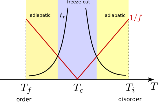
Figure 1: Qualitative illustration of the kz mechanism. We prepare the system initially in equilibrium at a certain temperature $T_{i}>T_{c}$ in the disordered phase. We then vary the temperature in time at a finite rate $f$ across the phase boundary up to a final value $T_{f}<T_{c}$. As long as the relaxation time $t_{r}<1/f$ the system adapts to the temperature variation and adiabatically follows the quench protocol (yellow regions). In the vicinity of the transition point, the divergence of $t_{r}$ leads to a time $\tau$ where $t_{r}=1/f$ after which the system cannot adjust to the temperature variation anymore and falls collectively out of equilibrium (blue region). The system remains frozen in this region until $t_{r}$ decays again in the ordered phase. This phenomenological picture can be better understood by means of finite time scaling [53, 54, 55].

The aim of this work is instead to extend the kz scaling theory to quench protocols across a first-order transition (fot). To do so, we consider a generic spin system which is known to show a phase transition from a magnetic down to up order, driven by an external magnetic field $h$ at a fixed temperature $T\leq T_{c}$, see figure 2. The nature of this transition depends on the temperature at which the magnetic transition is driven.

• At $T=T_{c}$ the transition is continuous and the standard kz scaling theory applies.

• For $T<T_{c}$ the transition is discontinuous and therefore the system correlation length remains finite at all times.

In the latter case, a new description is needed since the kz theory is built on the fact that the correlation length $\xi$ diverges at the critical point. Nevertheless, an equilibrium scaling theory has been developed for fots [56, 57, 58, 59] by replacing the correlation length with the coherence length $\xi_{h}$, which corresponds to the typical domain size of ordered clusters in minimal energy configuration. As soon as the discontinuous transition is approached, the two ordered phases become energetically indistinguishable, leading to a divergence of $\xi_{h}$. This divergence is physically reflected in magnetic systems by the long-range order arising in the spin-spin correlation function which asymptotically ($|\bm{x}-\bm{x}^{\prime}|\rightarrow\infty$) approaches the value of the squared magnetisation of the system [57]. Notice that the correlation length $\xi$ is instead defined by the connected part of the spin-spin correlator $G(\bm{x},\bm{x}^{\prime})\propto\exp\left(-|\bm{x}-\bm{x}^{\prime}|/\xi\right)$ and remains finite in the non-critical regime.

In this paper, we shall naturally extend this fot scaling theory to the non-equilibrium case à la kz and apply it to magnetic quench protocols in the ordered region as shown in figure 2 (green). This treatment is complementary to previous renormalisation group studies [60, 61, 62] and recent numerical evidence of dynamical scaling across fots [63].

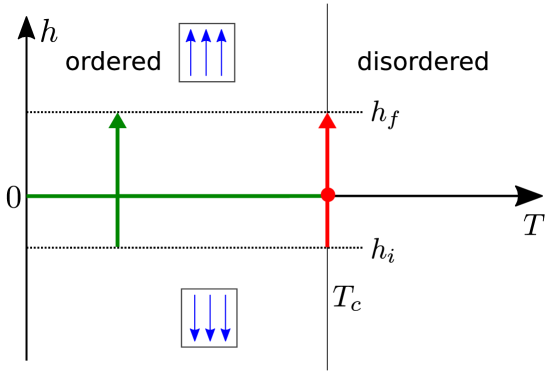
Figure 2: Schematic representation of the phase diagram for a generic spin system. The red dot indicates a continuous phase transition while the green line indicates a discontinuous transition. The corresponing arrows show qualitatively the quench protocols we shall study.

A theoretical framework for the description of generic spin systems is provided by the $O(n)$ model which is routinely cast as a field theory with the $n$-component vector field $\bm{\phi}(\bm{x})$ of unit norm and the action (see e.g. [64])

$$S[\bm{\phi}]=\frac{n}{2}\;\int{\rm d}\bm{x}\left[(\nabla\bm{\phi}(\bm{x}))^{2}+r\bm{\phi}^{2}(\bm{x})+u(\bm{\phi}^{2}(\bm{x}))^{2}-2\bm{h}\,\bm{\phi}(\bm{x})\right]$$ (1.1)

in $2<D<4$ spatial dimensions. Here, $u>0$ is a positive constant, $\bm{h}$ describes the external magnetic field and $r=r(T)$ is the thermal coupling constant. This model includes the celebrated Ising model ($n=1$), the xy model ($n=2$) and the Heisenberg model ($n=3$) as special cases [65]. In the particular case where $n\to\infty$, the bulk critical behaviour reduces to the one of the spherical model [66] and allows analytic investigation [67, 68, 69, 70, 71, 72, 73]. The analyticity in the large-$n$ limit arises due to the central limit theorem which implies that self-averaged $O(n)$ symmetric quantities are normally distributed for $n\to\infty$. This allows us to replace [74]

$$(\bm{\phi}^{2}(\bm{x}))^{2}\to\left<\bm{\phi}^{2}(\bm{x})\right>\bm{\phi}^{2}(\bm{x})$$ (1.2)

and cast the action in eq (1.1) quadratically

$$S[\bm{\phi}]=\frac{n}{2}\!\int\!{\rm d}\bm{x}\big{[}(\nabla\bm{\phi}(\bm{x}))^{2}\!+\!m^{2}\bm{\phi}^{2}(\bm{x})\!-\!2\bm{h}\,\bm{\phi}(\bm{x})\big{]}$$ (1.3)

with the effective mass

$$m^{2}=r+u\left<\bm{\phi}^{2}(\bm{x})\right>.$$ (1.4)

For this specific model, the $O(n)$ model at large $n$, we shall derive the structure of the off-equilibrium scaling functions of the magnetisation and of the transverse correlation functions. The latter are self-consistently related through an equation of state which describes - roughly speaking - the time-evolution of the magnetisation as a rotation generated by the dissipation of the initial equilibrium magnetisation into the transverse field modes (see section 3.2 for further details). We shall also provide a scaling prediction for the dissipated magnetic work $W$ during a round-trip protocol which takes the system across the fot and back. If we call the quench time scale $t_{s}$, one obtains in $D=3$ spatial dimensions

$$W\propto\begin{cases}t_{s}^{-2/3},\hskip 7.11317pt\text{for}\hskip 7.11317ptT=T_{c}\\[14.22636pt] t_{s}^{-1/2},\hskip 9.95863pt\text{for}\hskip 7.11317ptT<T_{c}\end{cases}\ .$$ (1.5)

Remarkably, these results apply beyond the large-$n$ limit with $2/3\approx 0.66$, as can be seen by a comparison with numerical results by Pelissetto and Vicari [75]. To complete our analysis, we shall numerically investigate the dynamics in the large-$n$ limit and explicitly test our scaling predictions.

The paper is organised as follows: After having set up the model in this introduction we turn to its general dynamical description in section 2. Here, we specify the magnetic quench protocol that we shall study and we determine the set of dynamical equations that describes the $O(n)$ model self-consistently for $n\to\infty$. In section 3 we then derive the dynamical scaling theory for the magnetic quench. We explicitly distinguish between (i) $T=T_{c}$ where we verify the kz scaling and (ii) $T<T_{c}$ where we develop a new out-of-equilibrium scaling theory. Finally, we apply these results in section 4 to a round-trip protocol for which we then derive the scaling behaviour of the hysteresis area and of the magnetic work performed over the cycle. We then briefly summarise our results and conclude the paper. Several technical aspects are described in the appendix.

2 Dynamical description of the $O(n)$ model

We want to describe the dynamics of the system (1.3) at and below the critical temperature $T_{c}$ when the external magnetic field is varied in time across the value $h_{c}=0$. We choose the linear ramp sketched in figure 3 along a fixed direction $\bm{e}_{1}$ which takes the system from a down order at initial time $t_{i}<0$ to an up order at the final time $t_{f}>0$, i.e.

$$\bm{h}(t)=\frac{t\ \bm{e}_{1}}{t_{f}-t_{i}}=t/t_{s}\,\bm{e}_{1}\ .$$ (2.1)

Here, $t_{s}=t_{f}-t_{i}$ defines the time-scale of the quench.

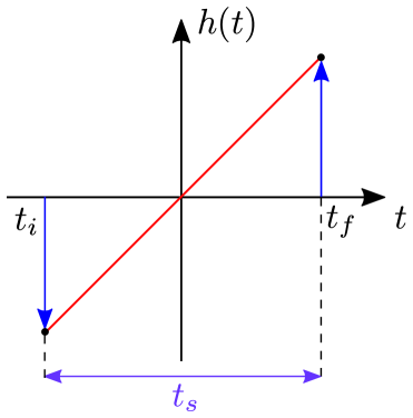
Figure 3: Schematic representation of the magnetic quench protocol (2.1). At initial time $t_{i}<0$ the system is in thermal equilibrium with the external magnetic field $h(t_{i})<0$. This field is then linearly driven through the magnetic transition point $h_{c}=0$ on a time scale $t_{s}$ until it reaches its final value $h(t_{f})>0$.

Within this convention, the critical value $h_{c}=0$ is reached at time $t=0$ which is but a convenient choice.

The dynamics of the components of the vector field is given by a Langevin equation

$$\partial_{t}\phi_{a}(\bm{x},t)=-\frac{\delta}{\delta\phi_{a}}S[\bm{\phi}]+\zeta_{a}(\bm{x},t)\ ,$$ (2.2)

where $\zeta_{a}(x,t)$ is a Gaussian white noise with zero mean, i.e.

$$\big{<}\zeta_{a}(\bm{x},t)\big{>} =0\ ,$$ (2.3)

$$\big{<}\zeta_{a}(\bm{x},t)\zeta_{b}(\bm{y},t^{\prime})\big{>} =2\delta_{a,b}\delta(\bm{x}-\bm{y})\delta(t-t^{\prime})\ .$$ (2.4)

The dynamics of the system is more involved than the one of a standard Gaussian theory due to eq (1.4) which has to be taken into account self-consistently. To do so, we first introduce the time-dependent magnetisation

$$\big{<}\phi_{a}(\bm{x},t)\big{>}=\delta_{1,a}\,M(t)$$ (2.5)

as order parameter of the transition. Moreover, we define the longitudinal and orthogonal (connected) correlation function as

$$G_{||}(x-y,t) \equiv\left<\Big{(}\phi_{1}(\bm{x},t)-\braket{\phi_{1}(\bm{x},t)}\Big{)}\Big{(}\phi_{1}(\bm{y},t)-\braket{\phi_{1}(\bm{y},t)}\Big{)}\right>\ ,$$ (2.6)

$$G_{\perp}(x-y,t) \equiv\left<\Big{(}\phi_{a}(\bm{x},t)-\braket{\phi_{a}(\bm{x},t)}\Big{)}\Big{(}\phi_{a}(\bm{y},t)-\braket{\phi_{a}(\bm{y},t)}\Big{)}\right>,\ a>1$$ (2.7)

Due to translational invariance, the dynamics is straightforwardly described in Fourier space and it is easy to show that it is governed by the following set of equations [77]

$$\frac{{\rm d}}{{\rm d}t}M(t) =-m^{2}(t)M(t)+h(t)\ ,$$ (2.8)

$$\partial_{t}G_{\perp}(\bm{q},t) =-2(m^{2}(t)+q^{2})G_{\perp}(\bm{q},t)+2\ ,$$ (2.9)

where the time-dependent effective mass $m(t)$ is defined through the equation of state

$$m^{2}(t)=r+u\bigg{[}M^{2}(t)+\int_{q}G_{\perp}({\bf q},t)\bigg{]}.$$ (2.10)

Here, we used the shorthand $\int_{q}=\int^{\Lambda}{\rm d}{\bf q}/(2\pi)^{d}$ with the momentum cut-off $\Lambda$. The dynamical eqs (2.8,2.9) can be formally solved as follows

$$M(t) =M_{0}\,\exp\bigg{[}-\int_{t_{i}}^{t}{\rm d}u\,m^{2}(u)\bigg{]}+\int_{t_{i}}^{t}{\rm d}u\,h(u)\,\exp\bigg{[}-\int_{u}^{t}{\rm d}s\,m^{2}(s)\bigg{]},$$ (2.11a)

$$G_{\perp}(\bm{q},t) =2\int_{t_{i}}^{t}{\rm d}u\exp\bigg{[}-2\int_{u}^{t}{\rm d}s\,\big{(}\bm{q}^{2}+m^{2}(s)\big{)}\bigg{]}\ ,$$ (2.11b)

with the initial equilibrium magnetisation $M_{0}$. In the following, we shall use these formal solutions (2.11a,2.11b) together with the equation of state (2.10) in order to describe the model out of equilibrium.

3 Dynamical scaling theory across phase transitions

In this section we develop a scaling theory à la kz for fots in order to describe the magnetic quench specified in eq (2.1). We shall though first start with the instructive case $T=T_{c}$ in section 3.1 in order to illustrate the standard kz theory for continuous transitions. We then turn to the case $T<T_{c}$ in section 3.2 where we shall develop the non-equilibrium scaling theory for fots.

Along with our scaling analysis, we shall provide numerical solutions of the dynamical equations of the $O(\infty)$ model $(\ref{dyn-obs},\ref{dyn-obsG},\ref{time-eq-state})$ and we shall use these results to check our scaling predictions. The numerical calculations will be carried out in $D=3$ spatial dimensions and with the normalisation $u=1$ which implies $r_{c}\simeq-0.051$ [77, 76]. For further details on the numerical method, see appendix D.

3.1 Scaling theory for the continuous transition ($T=T_{c}$)

In this case the standard kz scaling theory [27, 30] describes the universal scaling behaviour of the dynamics driven by the protocol (2.1). First, we have to express the correlation length $\xi$ close to the critical point $h_{c}=0$ as a power-law of the control parameter [76]

$$\xi(t)\sim|h(t)|^{-\nu_{h}},\;\;h\rightarrow 0$$ (3.1)

with the equilibrium critical exponent

$$\nu_{h}=\frac{1}{d_{h}}=\frac{2}{D+2}\ .$$ (3.2)

From $\xi$ in eq (3.1) we can define the typical time scale on which the system adapts to the variation of the magnetic field via $t_{\text{ad}}(t)=\xi/\dot{\xi}$ and compare it to the relaxation time associated with $\xi$ via $t_{\text{r}}(t)\sim\xi^{z}$, where $z=2$ is the dynamical critical exponent [79]. These time scales do compete during the quench as the system tries to relax towards equilibrium and to follow the quench protocol simultaneously. The Ansatz that underlies the kz approximation is that the system manages to equilibrate and to follow the quench adiabatically as long as $t_{\text{ad}}<t_{\text{r}}$, compare figure 1. In the opposite situation $t_{\text{ad}}>t_{\text{r}}$ the system cannot adapt to external changes anymore and is assumed to freeze out. The crossover time $\tau$ at which the system falls collectively out of equilibrium is then given by

$$t_{\text{ad}}(\tau)\stackrel{{\scriptstyle!}}{{=}}t_{\text{r}}(\tau)\;\Rightarrow\;\tau=t_{s}^{\frac{z\nu_{h}}{1+z\nu_{h}}}\ .$$ (3.3)

From this, we define, in analogy to the equilibrium correlation length, a characteristic length scale $\ell$ via the dynamical exponent $z$, i.e.

$$\ell=\tau^{1/z}=t_{s}^{\frac{\nu_{h}}{1+z\nu_{h}}}\ .$$ (3.4)

This length scale encodes the characteristic distance on which the system is correlated and thus allows us to study the non-equilibrium regime in a scaling limit. In this kz scaling regime, the quench is assumed to be slow $t_{s}\to\infty$ while $t/\tau$ and $q\,\ell$ are kept constant. It is well-known that the time-dependent correlation functions exhibit dynamical scaling behaviour for $h\rightarrow 0$ [76]

$$M(t)\sim\ell^{-d_{\phi}}\;\mathcal{M}(t/\tau)\ ,$$ (3.5a)

$$G_{\perp}(\bm{q},t)\sim\ell^{2}\;\mathcal{G}_{\perp}(\bm{q}\,\ell,t/\tau)\ ,$$ (3.5b)

where $d_{\phi}=(D-2)/2$ is the scaling dimension of the order parameter $M$ and $\mathcal{M}(\cdot)$, $\mathcal{G}_{\perp}(\cdot)$ are generic scaling functions [7].

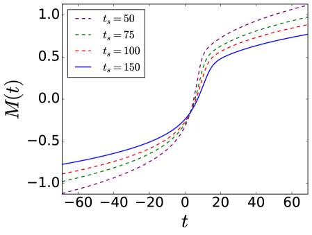
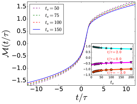
Figure 4: Numerical analysis of the dynamical magnetisation in $D=3$ spatial dimensions and at the critical temperature $T=T_{c}$. Left panel: magnetisation as a function of time for different quench times $t_{s}$, see eq (3.3). Right panel: data collapse and dynamical scaling function for the magnetisation (compare eq $\eqref{KZscaling-a}$). The inset shows the convergence of the scaling functions at finite $t_{s}$ towards the asymptotic regime ($t_{s}\rightarrow\infty$) for three different times.

We briefly comment that finite-size scaling can be implemented in this theory as well. For a system of finite size $L$, we would consider the limit $L,t_{s}\rightarrow\infty$, $t\rightarrow 0$ such that $t/\tau$, $q\,\ell$ and $L/\ell$ are fixed. In this limit the time-dependent correlators present the scaling relations [7]

$$M(t,L)\sim L^{-d_{\phi}}\;\mathcal{M}(t/\tau,L/\ell)\ ,$$ (3.6a)

$$G_{\perp}(\bm{q},t,L)\sim L^{2}\;\mathcal{G}_{\perp}(\bm{q}\,\ell,t/\tau,L/\ell)\ ,$$ (3.6b)

such that the infinite-volume behaviour of $\eqref{KZscaling}$ is recovered for $L/\ell\rightarrow 0$ at fixed $q\,\ell$, $t/\tau$. Notice also that, by construction, these scaling relations match the equilibrium scaling behaviour for $|t|\rightarrow\tau$ (see appendix A).

From a dimensional analysis, it is clear that the effective mass term must scale as [76]

$$m^{2}(t)\sim\ell^{-2}\,\mathfrak{m}^{2}(t/\tau)$$ (3.7)

with a general scaling function $\mathfrak{m}(\cdot)$. From eq (2.11a), the magnetisation is then given as

$$\mathcal{M}(\bar{t})=\int_{-\infty}^{\bar{t}}{\rm d}u\,u\,\exp\bigg{[}\!\!-\!\int_{u}^{\bar{t}}{\rm d}s\,\mathfrak{m}^{2}(s)\bigg{]}$$ (3.8a)

and from eq (2.11b) the transverse two-point function reads

$$\mathcal{G}_{\perp}(\bar{\bm{q}},\bar{t})=2\int_{-\infty}^{\bar{t}}{\rm d}u\,\exp\bigg{[}-2\int_{u}^{\bar{t}}{\rm d}s\,(\bar{\bm{q}}^{2}+\mathfrak{m}^{2}(s))\bigg{]}$$ (3.8b)

with the rescaled time $\bar{t}=t/\tau$ and momentum $\bar{\bm{q}}=\bm{q}\,\ell$. The time evolution of the scaling functions is thus solely determined by the function $\mathfrak{m}^{2}$ which has to be found from eq $\eqref{time-eq-state}$

$$\mathcal{M}^{2}(\bar{t},\mathfrak{m})=\int_{\bar{\bm{q}}}(\mathcal{G}_{\perp}(\bar{\bm{q}},\bar{t},0)-\mathcal{G}_{\perp}(\bar{\bm{q}},\bar{t},\mathfrak{m}))$$ (3.9)

where the critical thermal coupling constant has been expressed in terms of the critical two-point function [74, 76]

$$r_{c}=-u\int_{q}\,G_{\perp}(\bm{q},t,0)\ .$$ (3.10)

The equation of state $\eqref{eq-state-critical}$ shows that the time evolution of the magnetisation is generated by a dissipation into the transverse field components. In other words, the deviations from equilibrium of the magnetisation and of the transverse correlations compensate each other.

In figure 4 we show the numerical result for the time evolution of the magnetisation at the critical temperature. The numerical analysis confirms our scaling predictions, since clearly, for increasing times $\tau\sim t_{s}^{\frac{z\nu_{h}}{1+z\nu_{h}}}$, the data collapse onto a master curve which represents the sought scaling function. Similar results are obtained for the zero mode correlation function and the for mass term, shown in figure 5 and 6 respectively.

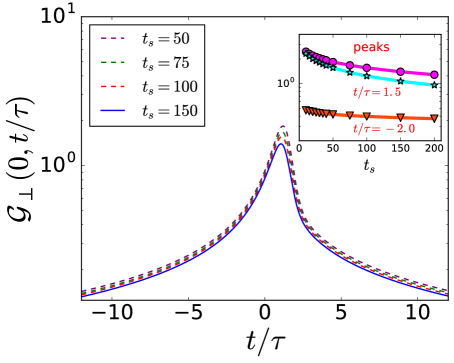
Figure 5: Numerical analysis of the zero mode correlation function at $T=T_{c}$ in $D=3$ spatial dimensions. We see the data in the left panel for different quench times $t_{s}$, see eq (3.3), and the data collapse (in log scale) for the dynamical scaling function in the right panel (compare eq $\eqref{KZscaling-b}$). The inset shows the convergence of the scaling functions at finite $t_{s}$ towards the asymptotic regime ($t_{s}\rightarrow\infty$) for three different times (the label “peaks” refers to the convergence of the maximum of the curves).

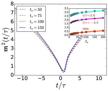
Figure 6: Numerical analysis of the effective mass at $T=T_{c}$ in $D=3$ dimensions. We see the data in the left panel for different quench times $t_{s}$ and the data collapse for the dynamical scaling function in the right panel (compare eq $\eqref{eq:mscalez2}$). The inset shows the convergence of the scaling functions at finite $t_{s}$ towards the asymptotic regime ($t_{s}\rightarrow\infty$) for three different times.

3.2 Scaling theory for fots ($T<T_{c}$)

In this section we argue that a kz-like theory can also be applied to the magnetic quench performed at $T<T_{c}$. The main obstacle for transferring the kz scaling theory to the fot below $T_{c}$ is that the system correlation length remains finite. We shall therefore turn to another length scale, the so-called coherence length or persistent length $\xi_{h}$ [57] which may be defined as the typical size of domains of (aligned) spins in the minimum energy configuration.

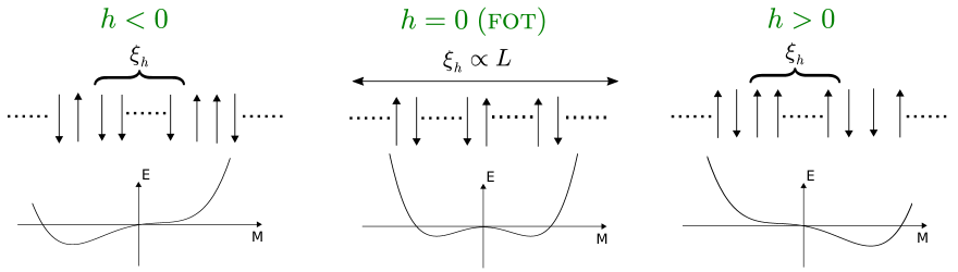
Figure 7: Visualisation of the coherence length $\xi_{h}$ and the associated Ginzburg-Landau functional $E$ as a function of the order parameter $M$ for a generic spin system. The different pictures show the variation of $\xi_{H}$ and $E$ during the protocol described in eq $\eqref{eq:quench}$. At the fot $h=0$, the degeneracy of the two vacua associated to the different realisations of the ordered phase leads to a divergence of $\xi_{h}$.

For $h\rightarrow 0$, the system cannot energetically distinguish between the two ordered phases and long-range order arises which leads to an increase of the coherence length. Eventually, this results in a macroscopic coherence length $\xi_{h}\propto L$, see figure 7.

In order to construct the scaling theory, we need to know the scaling behaviour of the coherence length as a function of the magnetic field in analogy to eq (3.1) and the dynamical exponent $z$. It is well-known that the behaviour of $\xi_{h}$ close to the fot can be expressed as a power-law [56, 57, 58, 59]

$$\xi_{h}(t)\sim|h(t)|^{-1/D}\ \ ,\ \ h\rightarrow 0$$ (3.11)

from which we can identify the critical exponent

$$\nu_{h}=1/D\,.$$ (3.12)

For the dynamical exponent $z$, a lengthy but straightforward calculation reveals

$$z=D\ ,$$ (3.13)

which can be qualitatively understood as follows. Initially, the equilibrium magnetisation is aligned with the initial magnetic field $h<0$. As this field is driven across the critical value $h_{c}=0$, the magnetisation has to flip in order to align with the final magnetic field $h>0$. Therefore, the vector of the magnetisation has to perform a rotation which needs a characteristic time of the order of the system volume $L^{D}$[75]. For further details on how to determine $z$ in the low temperature regime, we refer to appendix B.

We are now able to draw the analogy to eq (3.3), i.e. the freeze-out condition reveals

$$\tau_{\text{\sc fot}}=\sqrt{t_{s}},\qquad\ell_{\text{\sc fot}}=t_{s}^{1/2D}.$$ (3.14)

We notice that the freeze-out time $\tau_{\text{\sc fot}}$ coincides with the coercive time of the model [80] that is the typical time scale after which a ferromagnet reacts to an inversion of the external magnetic field.

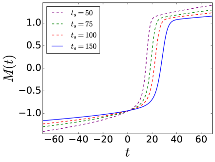
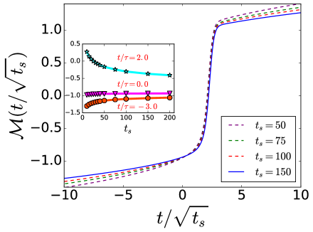
Figure 8: Numerical analysis of the dynamical magnetisation below $T_{c}$ ($r=-1$) in $D=3$ spatial dimensions. Left panel: dynamical magnetisation as a function of time for different quench time scales $t_{s}$. Right panel: data collapse and dynamical scaling function for the magnetisation (compare eq $\eqref{scaling-fot}$). The inset shows the convergence of the scaling functions at finite $t_{s}$ towards the asymptotic regime ($t_{s}\rightarrow\infty$) for three different times.

Extending this analogy further, we assume that the time-dependent magnetisation of the system in the vicinity of the transition point $h\to 0$ shows dynamical scaling behaviour in line with eq (3.5) in the limit $t_{s}\to\infty$ (with $t/\tau_{\text{\sc fot}}$ fixed)

$$M(t)\sim\ell_{\text{\sc fot}}^{-d_{\phi}}\;\mathcal{M}(t/\tau_{\text{\sc fot}})\ ,\\$$ (3.15)

where the scaling dimension of the order parameter is known to be $d_{\phi}=0$ [57]. The numerical result for the dynamical magnetisation below the critical temperature is shown in figure 8 and explicitly verifies our scaling prediction (3.15).

We describe our model in the spin-wave approximation [81, 82] which states that at low-temperatures $T<T_{c}$ it is sufficient to study long-range excitations, i.e. only the degrees of freedom with $|\bm{q}|<q^{\ast}$ turn out to be relevant for the off-equilibrium dynamics. The boundary value $q^{\ast}$ which separates the short-distance fluctuations $|\bm{q}|>q^{\ast}$ from the low-energy modes $|\bm{q}|<q^{\ast}$ can be estimated as $q^{\ast}\propto t_{s}^{-1/4}$, see appendix C. In the scaling limit $h\rightarrow 0$, $t_{s}\rightarrow\infty$ keeping $q\,\ell_{\text{\sc fot}}$ fixed we notice that

$$|\bm{q}|\,\ell_{\text{\sc fot}}<q^{\ast}\,\ell_{\text{\sc fot}}\propto t_{s}^{\frac{2-D}{4D}}\rightarrow 0\ ,$$ (3.16)

which implies that the zero-momentum contribution alone provides a good description of the off-equilibrium behaviour arising during the quench in the asymptotic limit. We introduce therefore the transverse susceptibility $\chi_{\perp}$ that obeys the scaling relation

$$\chi_{\perp}(t)\equiv G_{\perp}(\bm{0},t)\sim\ell_{\text{\sc fot}}^{D}\,\mathcal{X}_{\perp}(\bar{t})\ ,$$ (3.17)

as shown in figure 9. Notice that, by construction, the off-equilibrium scaling behaviours (3.15,3.17) match again the equilibrium scaling when $|t|\rightarrow\tau_{\text{\sc fot}}$ (see appendix A).

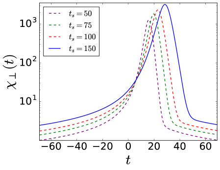
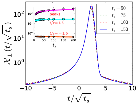
Figure 9: Numerical analysis of the transverse susceptibility below $T_{c}$ ($r=-1$) in $D=3$ spatial dimensions. In the left panel, the data for different quench times $t_{s}$ is shown in log scale and the right panel shows the data collapse for the dynamical scaling function (compare eq $\eqref{scal-G-low}$). The inset shows the convergence of the scaling functions at finite $t_{s}$ towards the asymptotic regime ($t_{s}\rightarrow\infty$) for three different times.

For the effective mass we write the analogous scaling behaviour to eq (3.7)

$$m^{2}(t)\sim\ell_{\text{\sc fot}}^{-D}\;\mathfrak{m}^{2}(t/\tau_{\text{\sc fot}})$$ (3.18)

due to the presence of a small magnetic field with scaling dimension $d_{h}=D$. The numerical result for the effective mass is shown in figure 10.

The time-dependent magnetisation satisfies the (trivial) scaling relation in eq $\eqref{scaling-fot}$ with the scaling function

$$M(t)\equiv\mathcal{M}(\bar{t})=\int_{-\infty}^{\bar{t}}{\rm d}s\,s\,\exp\bigg{[}-\int_{s}^{\bar{t}}\!{\rm d}u\,\mathfrak{m}^{2}(u)\bigg{]},$$ (3.19)

while the scaling function of the transverse susceptibility reads

$$\mathcal{X}_{\perp}(\bar{t})=2\int_{-\infty}^{\bar{t}}{\rm d}s\,\exp\bigg{[}-2\int_{s}^{\bar{t}}{\rm d}u\,\mathfrak{m}^{2}(u)\bigg{]}\ ,$$ (3.20)

where now $\bar{t}=t/\tau_{\text{\sc fot}}$ was redefined. In the spin-wave approximation we introduce the quantity

$$\mathscr{S}(t)=\int_{q}\,G_{\perp}(|\bm{q}|<q^{\ast},t)\sim{\cal S}(t/\tau_{\text{\sc fot}})$$ (3.21)

with a trivial scaling relation that follows from eq $\eqref{chi-low}$.

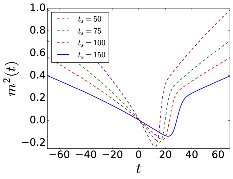
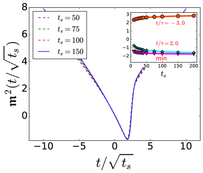
Figure 10: Numerical analysis of the effective mass below $T_{c}$ ($r=-1$). We see the data in the left panel for different quench times $t_{s}$ and the data collapse for the dynamical scaling function in the right panel (compare eq $\eqref{eq:mfot}$). Notice that the effective mass term can also take negative values below $T_{c}$, see also [80]. This is not surprising in the presence of a broken symmetry and refers to the formation and the propagation of massless modes who connects degenerate vacua, see e.g. [64]. The inset shows the convergence of the scaling functions at finite $t_{s}$ towards the asymptotic regime ($t_{s}\rightarrow\infty$) for three different times.

Notice that once again the scaling functions above depend implicitly on $\mathfrak{m}^{2}$ via the equation of state $\eqref{time-eq-state}$ which in the scaling limit and for $T<T_{c}$ reads

$$M_{0}^{2}={\cal M}^{2}(\bar{t},\mathfrak{m})+\mathcal{S}(\bar{t},\mathfrak{m})-\mathcal{S}(\bar{t},0)\ ,$$ (3.22)

where we have expressed the thermal coupling $r<r_{c}$ as

$$r=-u\left(M_{0}^{2}+\mathscr{S}(t,0)\right).$$ (3.23)

Eq $\eqref{eq-state-below}$ states that the magnetisation deviates from its equilibrium value $|M_{0}|=\sqrt{(r_{c}-r)/u}$ (see e.g. [64]) by dissipating in the transverse modes. The magnetisation may be viewed as a $n$-vector $M_{a}(t)\equiv\braket{\phi_{a}(\bm{x},t)}$ whose longitudinal component $M(t)$ in eq $\eqref{eq:M-t}$ is coupled to the other components $M_{a}(t)$, $a>1$, through the transverse correlation function. For weak magnetic fields, we may interpret the magnetisation as a $n$-vector of fixed length $|M_{0}|$ whose longitudinal component $M$ is decreased in favour of the transverse modes. The dynamical behaviour across the transition point is then nothing but a rotation of this vector. Moreover, this kind of dynamics is compatible with the $O(n-1)$ symmetry, because the $n-1$ transverse planes are equally likely to contain the vector magnetisation at any time. One may also verify that the definition of the scales $\eqref{scales-fot}$ is the only compatible with the dynamics $z=D$ that preserves the equilibrium limit at $|t|\rightarrow\tau_{\text{\sc fot}}$.

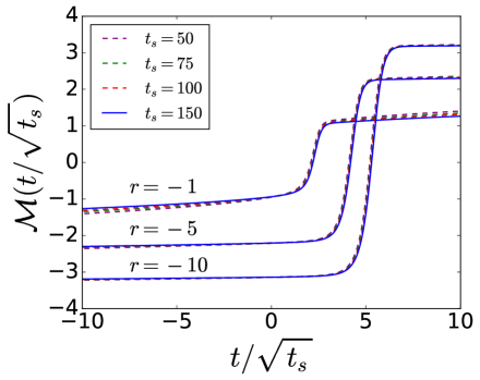
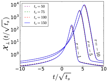
Figure 11: Off-equilibrium scaling behaviour of the magnetisation (left panel) and of the transverse susceptibility (right panel) for different values of the temperature ($r=-1,\,-5,\,-10$) below the critical value in $D=3$ spatial dimensions. The data collapse is observed for each value of the temperature confirming that the scaling behaviour is not modified by the specific value of $T<T_{c}$ considered.

In figure 11 we numerically investigate the off-equilibrium scaling across the fot for different values of the temperature $T<T_{c}$. As expected from phase kinetic arguments [11], the scaling theory does not depend on the specific value of the temperature considered.

4 Hysteresis in the round-trip protocol

In this section, we consider a round-trip protocol $\gamma(h)$ in which the magnetic field $\eqref{eq:quench}$ is varied from an initial value $h(t_{i})<0$ to $h(t_{f})>0$ across the transition point $h_{c}=0$ at $t=0$ and back in the reversed manner. By integrating the curve described by the magnetisation in time $\eqref{eq:M-t}$ over $\gamma(h)$ we obtain the hysteresis loop area $A$

$$A\equiv \oint_{\gamma(h)}{\rm d}t\;M(t)=\ 2\int_{t_{i}}^{t_{f}}{\rm d}t\,\int_{t_{i}}^{t}{\rm d}u\,h(u)\cosh\bigg{[}\int_{u}^{t}{\rm d}s\,m^{2}(s)\bigg{]}$$ (4.1)

which is a quantifier of the deviation from equilibrium during the process [75, 83]: the larger the deviations from equilibrium are, the larger is the value of $A$, while for a system in equilibrium $A=0$ since the magnetisation only depends on the instantaneous value of the external field. The hysteresis loop area $A$ is related to the magnetic energy $W$ dissipated by the system during the round trip. For a linear quench $\eqref{eq:quench}$ we have

$$W\equiv\oint_{\gamma(h)}{\rm d}h\;M(h)=\frac{A}{t_{s}}\;.$$ (4.2)

For further considerations, we shall work in the scaling limit $t_{s}\rightarrow\infty$, $h\rightarrow 0$ at $\bar{t}$, $|\bar{\bm{q}}|$ fixed (where we refer to the definitions $\eqref{ell}$ for $T=T_{c}$ and $\eqref{scales-fot}$ $T<T_{c}$ respectively).

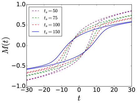
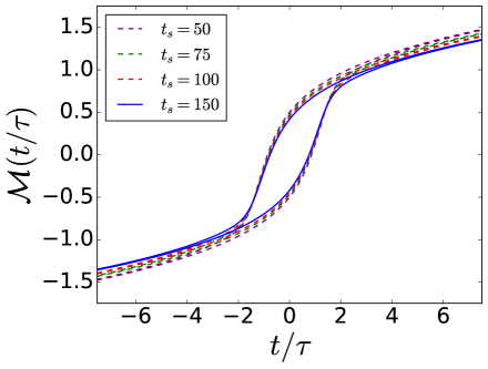
Figure 12: Numerical analysis of the dynamical magnetisation at $T_{c}$ during a round-trip protocol in $D=3$ spatial dimensions. Left panel: hysteresis loop area for different quench time scales $t_{s}$. Right panel: data collapse and dynamical scaling of the hysteresis area (compare eq $\eqref{scal-hyst-tc}$)

At the critical temperature $T=T_{c}$ the hysteresis loop area scales as

$$A\sim\ell^{z-d_{\phi}}\,\mathcal{A}\sim t_{s}^{\frac{6-D}{6+D}}\,\mathcal{A}\ ,$$ (4.3)

where the constant $\mathcal{A}$ reads

$$\mathcal{A}\!=2\!\int_{-\infty}^{+\infty}\!\!\!{\rm d}\bar{t}\int_{-\infty}^{\bar{t}}\!\!\!{\rm d}s\,s\cosh\!\bigg{[}\!\int_{s}^{\bar{t}}\!{\rm d}u\;\mathfrak{m}^{2}(u)\bigg{]}\ .$$ (4.4)

Consequently, the dissipated energy (in form of magnetic work) $W$ in $D=3$ spatial dimensions obeys the scaling relation

$$W\sim t_{s}^{-2/3}\,\mathcal{A}\ ,$$ (4.5)

i.e. the slower the protocol is performed, the less energy is dissipated during the round-trip protocol. This can be intuitively understood since the system will stay longer in equilibrium for a slow quench.

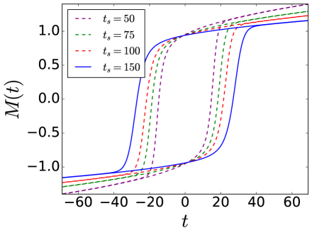
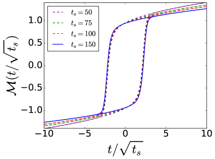
Figure 13: Numerical analysis of the dynamical magnetisation below $T_{c}$ ($r=-1$) during a round-trip protocol in $D=3$ spatial dimensions. Left panel: hysteresis loop area for different quench time scales $t_{s}$. Right panel: data collapse and dynamical scaling of the hysteresis area (compare eq $\eqref{scal-hyst-low}$)

Applying the same arguments to the magnetic fot below the thermal critical point $T<T_{c}$ we obtain for the hysteresis loop

$$A\sim\ell^{D}_{\text{\sc fot}}\;\mathcal{A}\sim\sqrt{t_{s}}\,{\cal A}$$ (4.6)

where the factor ${\cal A}$ has the same structure as $\eqref{hyst-scal-funct}$ in terms of the quantities at low temperature. For the magnetic work, we find the scaling relation

$$W\sim\ell_{\text{\sc fot}}^{-D}\;\mathcal{A}=\frac{\mathcal{A}}{\sqrt{t_{s}}}$$ (4.7)

independently from the spatial dimensions $2<D<4$. Numerical results for the hysteresis loop area are given in the figures 12 and 13, respectively for the cases $T=T_{c}$ and $T<T_{c}$.

The scaling relations in eqs (4.5,4.7) apply beyond the spherical limit $n\rightarrow\infty$ and are in agreement with the numerically obtained scaling behaviour for a $3D$ Heisenberg ferromagnet [75]. Indeed, in the case $T<T_{c}$, we showed that the dynamics is independent on the number of transverse components (see appendix B) while at the criticality $T=T_{c}$ the critical exponents of the $O(n)$ universality classes weakly depend on the rg exponent $\eta$ (see table 1) so that the large-$n$ limit provides a reliable guideline. In this sense, we can conclude that the scaling behaviour of the system is not modified by considering a finite number of components $n\geq 2$. The off-equilibrium scaling relations presented in this work are briefly summarised in table 2 for a generic $O(n\geq 2)$ model.

Table 1: Numerical estimations of the critical exponent $\eta$ for different universality classes in three spatial dimensions [84].

universality class	$\eta$	Ref.
XY	$0.0380(4)$	[85]
Heisenberg	$0.0375(5)$	[86]
$O(4)$	$0.0365(10)$	[87]
$O(\infty)$	$0$	e.g. [70]

Table 2: Off-equilibrium scaling relations for the $O(n)$ universality class with $n\geq 2$ during a magnetic quench $\eqref{eq:quench}$: at the continuous transition $T=T_{c}$ with $d_{\phi}=\frac{1}{2}\left(D-2+\eta\right)$, $\nu_{h}=1/(D-d_{\phi})$ and $z=2-\eta$ and for $T<T_{c}$.

observable	scaling $\;T=T_{c}$	scaling $T<T_{c}$
magnetisation $M(t)$	$\sim\ell^{-d_{\phi}}\,{\cal M}(t/\tau)$	$\sim t_{s}^{0}\,{\cal M}(t/\sqrt{t_{s}})$
trans. susceptibility $\chi_{\perp}(t)$	$\sim\ell^{2-\eta}\,\mathcal{X}_{\perp}(t/\tau)$	$\sim t_{s}^{1/2}\,\mathcal{X}_{\perp}(t/\sqrt{t_{s}})$
hysteresis area $A$	$\sim\ell^{z-d_{\phi}}\,{\cal A}$	$\sim t_{s}^{1/2}\,{\cal A}$

5 Summary and conclusion

We investigated the off-equilibrium scaling arising in classical spin systems due to the presence of a time-dependent magnetic field $h(t)=t/t_{s}$ which drives the system from an initial equilibrium state across the transition point $h_{c}=0$ at constant temperature $T\leq T_{c}$. In particular, we considered a system with $O(n)$ symmetry in the large-$n$ limit and in $2<D<4$ spatial dimensions. We analysed the two distinct scenarios $T=T_{c}$ and $T<T_{c}$ which are qualitatively different since the magnetic transition is continuous at $T=T_{c}$ and discontinuous for $T<T_{c}$.

After recalling the general features of the kz scaling for a continuous transition, we focused on the protocol below the critical temperature. Here, in the absence of a diverging correlation length, an equilibrium scaling theory is routinely formulate by referring to the coherence length $\xi_{h}$ as the characteristic scale. We extended this equilibrium theory to the non-equilibrium case by following the general ideas of the kz approach. To do so, we deduced several equilibrium exponents such as e.g. the dynamical exponent $z=D$ for the fot, needed to formulate the off-equilibrium scaling theory. As a result, thermodynamic observables such as the magnetisation or the magnetic susceptibility present dynamical scaling relations in terms of appropriate off-equilibrium scales. The latter are functions of the quench time scale $t_{s}$ and depend on the set of static and dynamic fot exponents. Quite remarkably, these scaling relations have the same structure as those at $T=T_{c}$ but with different exponents.

We then applied this scaling theory to a round-trip protocol, where we proposed the hysteresis area as a quantifier of the deviation from equilibrium and we derived its scaling behaviour. Moreover, the hysteresis can be easily connected to the dissipated magnetic energy by the system during a protocol and therefore with an energy cost.

As mentioned, all results presented in this work are derived in the large-$n$ limit. However, we argued that the dynamics of the system is not affected by the number of transverse components so that our results apply for any finite $n\geq 2$, as confirmed by a comparison with numerical studies [75].

Although there are several works on the dynamical off-equilibrium scaling at fots, e.g. in [88] where thermal quenches are analysed and in [89, 90, 91] where finite-size scaling in quantum systems is discussed, the study of non-equilibrium behaviour at fots is much less understood and investigated than its continuous counterpart. We do therefore believe that the simple and clear physical picture that the kz mechanism provides, opens new perspectives to this field of research which becomes experimentally more and more relevant, especially in the light of recent experiments in the area of ultracold atoms, where fots can be generated and studied systematically [50, 92, 93, 94, 22].

A next step might be the extension of the present work to a system with inhomogeneities, for which the continuous counterpart is already analysed in the literature e.g. [95, 96, 97]. The latter case is closely related to real experimental setups where ultracold atomic gases typically do not have a flat density profile due to the effects of a trapping potential [98, 99, 100].

Acknowledgements: SW is grateful to the LPCT Nancy for their warm hospitality. The authors would like to thank Ettore Vicari for his support during the development of this work. We appreciate fruitful discussions with Dragi Karevski and Malte Henkel and are thankful for their critical remarks on the manuscript. Furthermore, we would like to thank the referee for his or her careful reading and useful comments on the manuscript.

Appendix A Equilibrium limit

In this appendix we provide further details on how the off-equilibrium scaling behaviour (3.6) and (3.15) match their equilibrium counterparts. Therefore, we have to distinguish $T=T_{c}$ and $T<T_{c}$.

A.1 The continuous transition ($T=T_{c}$)

By construction, in equilibrium we can identify the effective mass term of the system with the inverse of the square of the instantaneous correlation length obtaining

$$\mathfrak{m}^{2}(t/\tau)\propto|t/\tau|^{2\nu_{h}}\,.$$ (A.1)

Notice that this kind of behaviour for $\mathfrak{m}^{2}(\cdot)$ provides an exponential suppression of the initial conditions in $\eqref{eq:M-t}$ and ensures the universality of the scaling behaviour [76]. The assumption $\eqref{eq-mass}$ can be easily checked as follows. The equilibrium scaling behaviour can be defined as the limit $\xi\rightarrow\infty$ at fixed $t/\xi^{z}$ for which the magnetisation $\eqref{eq:M-t}$ shows the behaviour

$$M(t)\sim\xi^{-d_{\phi}}(t)\;M_{0}\ ,$$ (A.2)

where $M_{0}$ is a constant. On the other hand the equilibrium matching at $|t|\rightarrow\tau$ imposes that

$$M(t)\sim\ell^{-d_{\phi}}\;\mathcal{M}(t/\tau)\ .$$ (A.3)

Therefore the scaling function $\eqref{scal-M}$ must satisfy

$$\lim_{t\rightarrow-\tau}\mathcal{M}(t/\tau)=M_{0}\,|t/\tau|^{1/\delta},$$ (A.4)

with $\delta=d_{h}/d_{\phi}$ being the equilibrium critical exponent. One may verify that by inserting the Ansatz $\eqref{eq-mass}$ into $\eqref{scal-M}$, a direct calculation gives the result $\eqref{match}$. With the same method we can derive for the transverse susceptibility

$$\lim_{t\rightarrow-\tau}\chi_{\perp}(t/\tau)\propto|t/\tau|^{-\gamma}\ ,$$ (A.5)

where $\gamma=2\nu_{h}$ is the equilibrium critical exponent for the system at large-$n$ [74].

A.2 The discontinuous transition ($T<T_{c}$)

Below the critical temperature and close enough to the transition point $h_{c}=0$, we can approximate the equilibrium value of the magnetisation by a constant $M_{0}=-\sqrt{(r-r_{c})/u}$ [80]. From this observation eq $\eqref{dyn-obs}$ gives for the effective mass

$$m^{2}(t)\approx\frac{h(t)}{M_{0}}\ ,$$ (A.6)

which becomes in the scaling limit

$$\mathfrak{m}^{2}(t/\tau_{\text{ \sc fot}})=\frac{t/\tau_{\text{ \sc fot}}}{M_{0}}\,.$$ (A.7)

By inserting $\eqref{eq-mass-low}$ in $\eqref{scal-M-low}$ we obtain for the magnetisation

$$\lim_{t\rightarrow-\tau_{\text{\sc fot}}}\mathcal{M}(t/\tau_{\text{ \sc fot}})=M_{0}\ .$$ (A.8)

Furthermore, a direct calculation of $\eqref{scal-G-low}$ using eq $\eqref{eq-mass-low}$ leads to

$$\chi_{\perp}(t)=\frac{M_{0}}{h(t)}\sim\ell^{D}_{\text{ \sc fot}}\,\frac{M_{0}}{t/\tau_{\text{ \sc fot}}}\;,$$ (A.9)

in agreement with the general predictions for the transverse susceptibility below the critical temperature [74].

Appendix B Dynamics at low temperature $T<T_{c}$

Here, we analyse the dynamical behaviour of the system in the regime $T<T_{c}$. The components $\phi_{a}(\bm{x},t)$ of the vector field satisfy the equation of motion $\eqref{dynamics}$

$$\partial_{t}\,\phi_{a}(\bm{x},t)=-\left(\nabla^{2}+m^{2}(t)\right)\phi_{a}(\bm{x},t)+\delta_{1,a}\,h(t)+\zeta_{a}(\bm{x},t)\,$$ (B.1)

from which we notice that all transverse components $a>1$ follow the same evolution. Hence, the number of transverse components does not influence the dynamics and all $n-1$ transverse planes are equivalent. It is thus useful to reduce the system to an $O(2)$ model [101] where the $2$-component vector field can be parametrised as

$$\phi(\bm{x},t)=|M_{0}|(1+r(\bm{x},t))\,\exp[i\theta(\bm{x},t)]\ ,$$ (B.2)

with a radial fluctuating field $r(\bm{x},t)$ and a dynamical phase $\theta(\bm{x},t)\in[0,2\pi)$. The equation of motion $\eqref{dynamics}$ is decomposed in a set of two coupled equations

$$\partial_{t}\,\theta(\bm{x},t)\,(1+r(\bm{x},t))=\nabla^{2}\theta(\bm{x},t)+2\nabla\theta(\bm{x},t)\nabla r(\bm{x},t) -\frac{h(t)}{|M_{0}|}\sin(\theta(\bm{x},t))+\zeta_{\theta}(\bm{x},t)\ ,$$ (B.3a)

$$\partial_{t}\,r(\bm{x},t)=\left(1+r(\bm{x},t)\right)\!(\nabla\theta(\bm{x},t))^{2}-m^{2}(t)\left(1+r(\bm{x},t)\right) +\frac{h(t)}{|M_{0}|}\cos(\theta(\bm{x},t))+\zeta_{r}(\bm{x},t)\ ,$$ (B.3b)

where now $\bm{x}=(x_{1},x_{2})$. We have redefined the white Gaussian noise $\eqref{noise}$ as

$$\zeta_{\theta}(\bm{x},t)\equiv\frac{1}{|M_{0}|}\big{(}-\zeta_{1}(\bm{x},t)\sin[\theta(\bm{x},t)]+\zeta_{2}(\bm{x},t)\cos[\theta(\bm{x},t)]\big{)}$$ (B.4)

for the angular motion, and

$$\zeta_{r}(\bm{x},t)\equiv\frac{1}{|M_{0}|}\big{(}\zeta_{1}(\bm{x},t)\cos[\theta(\bm{x},t)]+\zeta_{2}(\bm{x},t)\sin[\theta(\bm{x},t)]\big{)}$$ (B.5)

along the radial direction, both with zero mean and variance $2/M_{0}^{2}$.

We shall consider the following approximations:

1. Radial fluctuations are negligible $(1+r)\approx 1$, which provides a good description for weak magnetic fields at low temperatures.

2. The angular and radial degrees of freedom are decoupled $\braket{\nabla\theta\cdot\nabla r}=0$.

3. The kinetic term is given by long wavelength modes $|\bm{q}|<q^{*}$ (see appendix C).

Under these assumptions the evolution of the dynamical phase is described in the Fourier space by

$$\partial_{t}\,\theta(\bm{q},t)=-\bm{q}^{2}\,\theta(\bm{q},t)-\frac{h(t)}{|M_{0}|}\sin(\theta(\bm{q},t))+\zeta_{\theta}(\bm{q},t),\qquad|\bm{q}|<q^{*}$$ (B.6)

where $\zeta_{\theta}(\bm{q},t)$ is the Fourier transform of the noise distribution having the same cumulants.

Eq $\eqref{phase-evo}$ shows two opposite regimes depending on the value of the magnetic field

$$\partial_{t}\,\theta(\bm{0},t) =-\frac{h(t)}{|M_{0}|}\sin(\theta(\bm{0},t))+\zeta_{\theta}(\bm{0},t)\ ,\hskip 56.9055pt\left|\frac{h(t)}{M_{0}}\right|\gg(q^{*})^{2}\simeq 0\ ,$$ (B.7a)

$$\partial_{t}\,\theta(\bm{q},t) =-\bm{q}^{2}\,\theta(\bm{q},t)+\zeta_{\theta}(\bm{q},t),\hskip 97.45078pt\left|\frac{h(t)}{M_{0}}\right|\ll(q^{*})^{2}\ .$$ (B.7b)

The former case corresponds to the equilibrium limit $|t|\gg\tau_{\text{\sc fot}}$ while the latter describes the off-equilibrium regime $|t|\ll\tau_{\text{\sc fot}}$. We shall refer to these two regimes with the shorthand notation $h\neq 0$ and $h=0$ respectively.

Case $h\neq 0$

We start by analysing the phase dynamics away from the transition point. Here, the time evolution is given by $\eqref{CASE1}$

$$\partial_{t}\,\theta(\bm{0},t)=-\frac{h(t)}{|M_{0}|}\sin(\theta(\bm{0},t))+\zeta_{\theta}(\bm{0},t)\ .$$ (B.8)

As we discussed in appendix A, in this regime the value of the magnetisation is not modified significantly. It is therefore convenient to consider the Taylor expansion of the phase $\theta(\bm{0},t)$ around the initial value $\theta(\bm{0},t_{i})=\pi$. At the leading order we obtain

$$\partial_{t}\,\vartheta(t)=\frac{h(t)}{|M_{0}|}\,\vartheta(t)+\zeta_{\theta}(t)$$ (B.9)

where $\vartheta(t)\equiv\theta(\bm{0},t)-\pi$ and with the formal solution

$$\vartheta(t)=\int_{t_{i}}^{t}{\rm d}u\,\exp\bigg{[}\int_{u}^{t}{\rm d}s\,\frac{h(s)}{|M_{0}|}\bigg{]}\,\zeta_{\theta}(u)\ .$$ (B.10)

The mean value of the phase is zero $\braket{\vartheta(t)}=0$ while its variance is

$$\sigma^{2}(t)\equiv\braket{(\vartheta(t)-\braket{\vartheta})^{2}}=\frac{2}{M_{0}^{2}}\,\exp\left[\frac{t^{2}}{|M_{0}|\,t_{s}}\right]\;\frac{\sqrt{\pi|M_{0}|t_{s}}}{2}\,\text{Erfc}\left[\frac{|t|}{\sqrt{|M_{0}|\,t_{s}}}\right]\ .$$ (B.11)

In the equilibrium limit $|t|\rightarrow\tau_{\text{\sc fot}}$ (in which the small-angle approximation holds) a straightforward calculation shows

$$\lim_{t\rightarrow-\tau_{\text{\sc fot}}}\sigma^{2}(t)=\frac{1}{M^{2}_{0}}\,\chi_{\perp}(t)\ .$$ (B.12)

The distribution $P(\vartheta,t)$ of the dynamical phase $\vartheta(t)$ can be derived solving the associated Fokker-Plank equation

$$\partial_{t}\,P(\vartheta,t)=-\frac{\delta}{\delta\vartheta}\left(\frac{h(t)}{|M_{0}|}\,\vartheta\,P(\vartheta,t)\right)+\frac{\delta^{2}}{\delta\vartheta^{2}}\,P(\vartheta,t)\ ,$$ (B.13)

with the initial condition $P(\vartheta,t_{0})=\delta(\vartheta)$ and having a standard gaussian solution

$$P(\vartheta,t)=\frac{1}{\sqrt{2\pi}\sigma^{2}(t)}\,\exp\left(-\frac{\vartheta^{2}}{2\sigma^{2}(t)}\right)\ .$$ (B.14)

In this regime, we conclude that the phase dynamics consists of Gaussian fluctuations ($z=2$) due to the transverse modes and it leaves the mean value of the magnetisation unchanged.

Case $h=0$

Here, we focus on the phase dynamics in the off-equilibrium regime. It is convenient to introduce a finite size $L$ in a way that, in absence of anisotropies, the volume of the system is $V=L^{D}$. In a finite-geometry the dynamical phase and its Fourier modes are related through

$$\theta(\bm{q},t)=\int_{V}d\bm{x}\;e^{i\bm{q}\,\bm{x}}\,\,\theta(\bm{x},t)\;,\qquad\theta(\bm{x},t)=\frac{1}{V}\sum_{q}e^{-i\bm{q}\,\bm{x}}\,\theta(\bm{q},t)\;.$$ (B.15)

The time-evolution of the phase is given by eq $\eqref{CASE2}$

$$\partial_{t}\,\theta(\bm{q},t)=-\bm{q}^{2}\,\theta(\bm{q},t)+\zeta_{\theta}(\bm{q},t)\ ,$$ (B.16)

having the formal solution

$$\theta(\bm{q},t)=e^{-\bm{q}^{2}\,t}\int_{t_{0}}^{t}{\rm d}u\,e^{\bm{q}^{2}u}\,\zeta_{\theta}(\bm{q},u)\ ,$$ (B.17)

where, without loss of generality, we assumed $\theta(\bm{q},t_{0})=0$. Using $\eqref{theta-h-0}$ and $\eqref{rep-low-temp}$, we are able to compute the autocorrelation function of the magnetisation

$$\braket{M(t)\;M(s)}\equiv\frac{M^{2}_{0}}{V}\int{\rm d}\bm{x}\,{\rm d}\bm{y}\braket{e^{i\theta(\bm{x},t)-i\theta(\bm{y},s)}}\ .$$ (B.18)

At this point, if we consider the spatial average of the dynamical phase

$$\Theta(t)\equiv\frac{1}{V}\int_{V}{\rm d}\bm{x}\;\theta(\bm{x},t)$$ (B.19)

such that $\theta(\bm{x},t)=\Theta(t)+\mathcal{O}(1/\sqrt{L})$, we may approximate the autocorrelation function $\eqref{autocorrM}$ as [75]

$$\braket{M(t)\;M(s)}\approx M^{2}_{0}\;\braket{e^{i\Theta(t)-i\Theta(s)}}=M_{0}^{2}\,\exp\left[-\frac{|t-s|}{M^{2}_{0}\,V}\right]$$ (B.20)

from which we deduce that the autocorrelation time is of the order of $L^{D}$ implying that the dynamical exponent is $z=D$.

Appendix C Spin-wave approximation

We consider the expression $\eqref{eq:GT-t}$ for the transverse correlation function

$$G_{\perp}(\bm{q},t)=2\int_{t_{0}}^{t}{\rm d}u\,\exp\bigg{[}-2\int_{u}^{t}{\rm d}s\,(\bm{q}^{2}+m^{2}(s))\bigg{]}.$$ (C.1)

As argued in appendix A, below the critical temperature and for weak magnetic fields $h\simeq 0$ the magnetisation can be approximated by its equilibrium value $M_{0}$. In this approximation scheme, we obtain the estimate of the mass term $\eqref{eq-mass-low}$. We already know that this approximation breaks down when $|t|\leq\tau_{\text{\sc fot}}$, where the magnetisation cannot be considered as constant anymore. However, the naive use of the Ansatz $\eqref{eq-mass-low}$ permits to compute the value of the transverse correlation function explicitly

$$G_{\perp}(\bm{q},t)\approx e^{s^{2}}\,\sqrt{\frac{\pi}{2}}\,\sqrt{|M_{0}|\,t_{s}}\,\Big{(}\text{Erfc}(s(\bm{q},t))-\text{Erfc}(s(\bm{q},t_{0}))\Big{)}\ ,$$ (C.2)

where $s(\bm{q},t)\equiv(\bm{q}^{2}\,|M_{0}|\,t_{s}+|t|)/\sqrt{|M_{0}|\,t_{s}}$. For large $s\gg 1$ the equilibrium propagator is recovered

$$\lim_{s\rightarrow\infty}G_{\perp}(s(\bm{q},t))=\frac{1}{\bm{q}^{2}+h(t)/M_{0}}=\frac{1}{\bm{q}^{2}+m^{2}(t)}\ .$$ (C.3)

Notice that the limit $s\to\infty$ does not necessarily imply $|t/\tau_{\text{\sc fot}}|\rightarrow\infty$, i.e. the equilibrium limit. Indeed, considering large momenta, the system appears at any time in equilibrium. We shall therefore consider for the non-equilibrium dynamics only long-wavelength fluctuations $|\bm{q}|<q^{*}$ while we assume that modes $|\bm{q}|>q^{*}$ are always in equilibrium. The boundary value $q^{*}$ which separates the two regimes can be obtained imposing the condition $s(q^{*},t=0)\sim\mathcal{O}(1)$ [80]. From the latter we have the estimation

$$q^{*}\propto t_{s}^{-1/4}\ .$$ (C.4)

Appendix D Numerical Implementation

The dynamical eqs (2.8,2.9,2.10) can be numerically solved using an iterative method, see e.g. [14]. We first divide the time-window of the protocol $t_{s}=t_{f}-t_{i}$ into ${\cal N}$ parts

$$k=\frac{t_{s}}{\cal N}\,,\qquad k\ll t_{s}$$ (D.1)

and we consider the discretised time variable $t^{(j)}=t_{i}+kj$, $j=0,\dots,{\cal N}$. Any function of time $f(t)$ may then be written in discretised version as a ${\cal N}+1$-vector

$$f(t)\;\longmapsto\;f=\begin{pmatrix}f_{0},\dots,f_{\cal N}\end{pmatrix}\,,\qquad f_{j}=f\left(t^{(j)}\right)$$ (D.2)

and the time derivative may be replaced by a finite difference

$$\frac{d}{dt}\,f(t)\;\longmapsto\;\frac{f_{j+1}-f_{j}}{k}\,,\quad\forall j\,.$$ (D.3)

We then have to consider the integral over the momenta of the transverse correlation function

$$\int_{\bm{q}}G_{\perp}(\bm{q},t)=\frac{\Omega_{D}}{(2\pi)^{D}}\int_{0}^{\Lambda}{\rm d}q\,q^{D-1}\,G_{\perp}(q,t)$$ (D.4)

since the transverse correlation function depends only on $|\bm{q}|$. To estimate this integral, we discretise the momenta

$$\kappa=\frac{\Lambda}{{\cal N}_{q}}\ ,\qquad\kappa\ll\Lambda$$ (D.5)

so that the discretised momentum is $q=\kappa z$, $z=0,\dots,{\cal N}_{q}$. Momentum integrations can then be evaluated as

$$\frac{\Omega_{D}}{(2\pi)^{D}}\int_{0}^{\Lambda}{\rm d}q\,q^{D-1}\,G_{\perp}(q,t)\approx\frac{\Omega_{D}}{(2\pi)^{D}}\,\kappa\left(\sum_{z=1}^{{\cal N}_{q}-1}\left(\kappa z\right)^{D-1}\,G_{\perp}(\kappa\,z,t)+\frac{1}{2}\Lambda^{D-1}\,G_{\perp}(\Lambda,t)\right)$$ (D.6)

using the extended trapezoidal rule [102]. The discretised versions of the eqs (2.8,2.9,2.10) then read

$$M_{j+1} =M_{j}+k\left[h_{j}-s_{j}\,M_{j}\right]$$ (D.7a)

$$g_{z,j+1} =g_{z,j}-2k\left[\left((\kappa z)^{2}+s_{j}\right)\,g_{z,j}-1\right]$$ (D.7b)

$$s_{j} =r+u\bigg{[}M_{j}^{2}+\frac{\Omega_{D}}{(2\pi)^{D}}\,\kappa\bigg{(}\sum_{z=1}^{{\cal N}_{q}-1}\left(\kappa z\right)^{D-1}\,g_{z,j}+\frac{\Lambda^{D-1}}{2}\,g_{{\cal N}_{q},j}\bigg{)}\bigg{]}$$ (D.7c)

with $M_{j}\equiv M(t^{(j)})$, $g_{z,j}\equiv G_{\perp}(\kappa z,t^{(j)})$, $s_{j}\equiv m^{2}(t^{(j)})$ and $h_{j}=t^{(j)}/t_{s}$. This set of algebraic equation can be solved iteratively starting from the initial equilibrium constraints

$$s_{0}=\frac{h_{0}}{M_{0}}\,,\qquad g_{z,0}=\frac{1}{\kappa^{2}z^{2}+s_{0}}$$ (D.8)

with $M_{0}$ given by $\eqref{eq3}$ for $j=0$. For simplicity, we focus on $D=3$ and we set $u=1$. The thermal critical coupling then reads $r_{c}=-1/2\pi^{2}\simeq-0.051$ and we can explore the cases $r=r_{c}$ and $r<r_{c}$ respectively.

References

- [1] Amit D. Field Theory, the Renormalization Group, and Critical Phenomena. International series in pure and applied physics. World Scientific (1984).
- [2] Cardy JL. Scaling and Renormalisation in Statistical Physics. Cambridge University Press, Cambridge (1996).
- [3] Sachdev S. Quantum Phase Transitions. Cambridge University Press (2001).
- [4] Nishimori H and Ortiz G. Elements of Phase Transitions and Critical Phenomena. Oxford Graduate Texts. Oxford University Press, Oxford (2011).
- [5] Wipf A. Statistical Approach to Quantum Field Theory, vol. 864 of Springer Lecture Notes in Physics. Springer, Heidelberg (2013).
- [6] Henkel M, Hinrichsen H and Lübeck S. Non-Equilibrium Phase Transitions: Volume 1: Absorbing Phase Transitions. Theoretical and Mathematical Physics. Springer, Heidelberg (2009).
- [7] Henkel M and Pleimling M. Non-Equilibrium Phase Transitions: Volume 2: Ageing and Dynamical Scaling Far from Equilibrium. Theoretical and Mathematical Physics. Springer, Heidelberg (2010).
- [8] Cugliandolo LF. In et al JLB (ed.), Slow Relaxations and Non-Equilibrium Dynamics in Condensed Matter (Les Houches LXXVII), 367–521. Springer, Heidelberg (2003). doi:10.1007/b80352.
- [9] Täuber UC. Critical Dynamics. Cambridge press (2014).
- [10] Struik LCE. Polymer Engineering & Science, 17(3):165 (1978). doi:10.1002/pen.760170305.
- [11] Bray A. Advances in Physics, 43(3):357 (1994). doi:10.1080/00018739400101505.
- [12] Cates M and Evans M. Soft and Fragile Matter: Nonequilibrium Dynamics, Metastability and Flow (PBK). Scottish Graduate Series. Taylor & Francis (2000).
- [13] Godrèche C and Luck JM. Journal of Physics: Condensed Matter, 14(7):1589 (2002). doi:10.1088/0953-8984/14/7/316.
- [14] Paessens M and Henkel M. Journal of Physics A: Mathematical and General, 36(34):8983 (2003). doi:10.1088/0305-4470/36/34/304.
- [15] Breuer H and Petruccione F. The Theory of Open Quantum Systems. Oxford University Press, Oxford (2007).
- [16] Schaller G. Open Quantum Systems Far from Equilibrium, vol. 881 of Lecture Notes in Physics. Springer International Publishing (2014).
- [17] Gagel P, Orth PP and Schmalian J. Phys Rev B, 92:115121 (2015). doi:10.1103/PhysRevB.92.115121.
- [18] Maraga A et al. Phys Rev E, 92:042151 (2015). doi:10.1103/PhysRevE.92.042151.
- [19] Chiocchetta A et al. Phys Rev Lett, 118:135701 (2017). doi:10.1103/PhysRevLett.118.135701.
- [20] Gagel P, Orth PP and Schmalian J. Phys Rev Lett, 113:220401 (2014). doi:10.1103/PhysRevLett.113.220401.
- [21] Wald S and Henkel M. Journal of Physics A: Mathematical and Theoretical, 49(12):125001 (2016). doi:10.1088/1751-8113/49/12/125001.
- [22] Wald S, Landi GT and Henkel M. Journal of Statistical Mechanics: Theory and Experiment, 2018(1):013103 (2018). doi:10.1088/1742-5468/aa9f44.
- [23] Wald S et al. Phys Rev A, 97:023608 (2018). doi:10.1103/PhysRevA.97.023608.
- [24] Gardiner C and Zoller P. Quantum Noise: A Handbook of Markovian and Non-Markovian Quantum Stochastic Methods with Applications to Quantum Optics. Springer Series in Synergetics. Springer (2004).
- [25] Godrèche C and Luck JM. Journal of Physics A: Mathematical and General, 33(50):9141 (2000). doi:10.1088/0305-4470/33/50/302.
- [26] Godrèche C and Luck JM. Journal of Statistical Mechanics: Theory and Experiment, 2013(05):P05006 (2013). doi:10.1088/1742-5468/2013/05/P05006.
- [27] Kibble TWB. Journal of Physics A: Mathematical and General, 9(8):1387 (1976). doi:10.1088/0305-4470/9/8/029.
- [28] Kibble TWB. Physics Reports, 67(1):183 (1980). doi:10.1016/0370-1573(80)90091-5.
- [29] Kibble TWB. Lectures at NATO ASI ”Patterns of symmetry breaking”, Cracow (2002).
- [30] Zurek WH. Nature, 317:505 (1985). doi:10.1038/317505a0.
- [31] Zurek WH. Physics Reports, 276(4):177 (1996). doi:10.1016/S0370-1573(96)00009-9.
- [32] Donadello S et al. Phys Rev A, 94:023628 (2016). doi:10.1103/PhysRevA.94.023628.
- [33] Lamporesi G et al. Nature Physics, 9:656 (2013). doi:10.1038/nphys2734.
- [34] Pyka K et al. Nature Communications, 4:2291 EP (2013). doi:/10.1038/ncomms3291.
- [35] Corman L et al. Phys Rev Lett, 113:135302 (2014). doi:10.1103/PhysRevLett.113.135302.
- [36] Cui JM et al. Scientific Reports, 6:33381 EP (2016). doi:10.1038/srep33381.
- [37] Calabrese P and Gambassi A. Phys Rev B, 66:212407 (2002). doi:10.1103/PhysRevB.66.212407.
- [38] Wald S and Henkel M. Integral Transforms and Special Functions, 29(2):95 (2018). doi:10.1080/10652469.2017.1404596.
- [39] Calabrese P and Gambassi A. Journal of Physics A: Mathematical and General, 38(18):R133 (2005). doi:doi.org/10.1088/0305-4470/38/18/R01.
- [40] Zurek WH, Dorner U and Zoller P. Phys Rev Lett, 95:105701 (2005). doi:10.1103/PhysRevLett.95.105701.
- [41] Polkovnikov A. Phys Rev B, 72:161201 (2005). doi:10.1103/PhysRevB.72.161201.
- [42] Dziarmaga J. Phys Rev Lett, 95:245701 (2005). doi:10.1103/PhysRevLett.95.245701.
- [43] Damski B. Phys Rev Lett, 95:035701 (2005). doi:10.1103/PhysRevLett.95.035701.
- [44] Dziarmaga J. Advances in Physics, 59(6):1063 (2010). doi:10.1080/00018732.2010.514702.
- [45] Polkovnikov A et al. Rev Mod Phys, 83:863 (2011). doi:10.1103/RevModPhys.83.863.
- [46] Beugnon J and Navon N. Journal of Physics B: Atomic, Molecular and Optical Physics, 50(2):022002 (2017). doi:10.1088/1361-6455/50/2/022002.
- [47] Zurek WH. Phys Rev Lett, 102:105702 (2009). doi:10.1103/PhysRevLett.102.105702.
- [48] Del Campo A, Retzker A and Plenio MB. New Journal of Physics, 13(8):083022 (2011). doi:10.1088/1367-2630/13/8/083022.
- [49] Scopa S and Karevski D. Journal of Physics A: Mathematical and Theoretical, 50(42):425301 (2017). doi:10.1088/1751-8121/aa890f.
- [50] Landig R et al. Nature, 532(7600):476 (2016). doi:10.1038/nature17409.
- [51] Hruby L et al. Proceedings of the National Academy of Sciences, 115(13):3279 (2018). doi:10.1073/pnas.1720415115.
- [52] Landini M et al. Phys Rev Lett, 120:223602 (2018). doi:10.1103/PhysRevLett.120.223602.
- [53] Huang Y et al. Phys Rev B, 90:134108 (2014). doi:10.1103/PhysRevB.90.134108.
- [54] Gong S et al. New Journal of Physics, 12(4):043036 (2010). doi:10.1088/1367-2630/12/4/043036.
- [55] Feng B, Yin S and Zhong F. Phys Rev B, 94:144103 (2016). doi:10.1103/PhysRevB.94.144103.
- [56] Nienhuis B and Nauenberg M. Phys Rev Lett, 35:477 (1975). doi:10.1103/PhysRevLett.35.477.
- [57] Fisher ME and Berker AN. Phys Rev B, 26:2507 (1982). doi:10.1103/PhysRevB.26.2507.
- [58] Privman ME Vladimirand Fisher. Journal of Statistical Physics, 33(2):385 (1983). doi:10.1007/BF01009803.
- [59] Binder K. Reports on Progress in Physics, 50(7):783 (1987). doi:10.1088/0034-4885/50/7/001.
- [60] Zhong F and Zhang J. Phys Rev Lett, 75:2027 (1995). doi:10.1103/PhysRevLett.75.2027.
- [61] Zhong F and Chen Q. Phys Rev Lett, 95:175701 (2005). doi:10.1103/PhysRevLett.95.175701.
- [62] Zhong F. Phys Rev E, 73:047102 (2006). doi:10.1103/PhysRevE.73.047102.
- [63] Zhong F. arXiv:1804.08514 (2018).
- [64] Zinn-Justin J. Quantum Field Theory and Critical Phenomena. Clarendon press - Oxford (2012).
- [65] Stanley HE. Phys Rev Lett, 20:589 (1968). doi:10.1103/PhysRevLett.20.589.
- [66] Stanley HE. Phys Rev, 176:718 (1968). doi:10.1103/PhysRev.176.718.
- [67] Baxter RJ. Exactly solved models in statistical mechanics. Academic Press, London (1982).
- [68] Oliveira MH, Raposo EP and Coutinho-Filho MD. Phys Rev B, 74:184101 (2006). doi:10.1103/PhysRevB.74.184101.
- [69] Vojta T. Physical Review B, 53(2):710 (1996). doi:10.1103/PhysRevB.53.710.
- [70] Berlin TH and Kac M. Phys Rev, 86:821 (1952). doi:10.1103/PhysRev.86.821.
- [71] Lewis HW and Wannier GH. Phys Rev, 88:682 (1952). doi:10.1103/PhysRev.88.682.2.
- [72] Wald S and Henkel M. Journal of Statistical Mechanics: Theory and Experiment, 2015(7):P07006 (2015). doi:10.1088/1742-5468/2015/07/P07006.
- [73] Henkel M and Hoeger C. Zeitschrift für Physik B Condensed Matter, 55(1):67 (1984). doi:10.1007/BF01307503.
- [74] Moshe M and Zinn-Justin J. Physics Reports, 385(3):69 (2003). doi:10.1016/S0370-1573(03)00263-1.
- [75] Pelissetto A and Vicari E. Phys Rev E, 93:032141 (2016). doi:10.1103/PhysRevE.93.032141.
- [76] Chandran A et al. Phys Rev B, 86:064304 (2012). doi:10.1103/PhysRevB.86.064304.
- [77] Mazenko GF and Zannetti M. Phys Rev B, 32:4565 (1985). doi:10.1103/PhysRevB.32.4565.
- [78] Guida R and Zinn-Justin J. Journal of Physics A: Mathematical and General, 31(40):8103 (1998). doi:10.1088/0305-4470/31/40/006.
- [79] Cardy J. Scaling and Renormalization in Statistical Physics. Cambridge press (1996).
- [80] Dhar D and Thomas PB. Journal of Physics A: Mathematical and General, 25(19):4967 (1992). doi:10.1088/0305-4470/25/19/012.
- [81] Bloch F. Zeitschrift für Physik, 61(3):206 (1930). doi:10.1007/BF01339661.
- [82] Bloch F. Zeitschrift für Physik, 74(5):295 (1932). doi:10.1007/BF01337791.
- [83] Hamp J et al. Phys Rev B, 92:075142 (2015). doi:10.1103/PhysRevB.92.075142.
- [84] Pelissetto A and Vicari E. Physics Reports, 368(6):549 (2002). doi:10.1016/S0370-1573(02)00219-3.
- [85] Campostrini M et al. Phys Rev B, 63:214503 (2001). doi:10.1103/PhysRevB.63.214503.
- [86] Campostrini M et al. Phys Rev B, 65:144520 (2002). doi:10.1103/PhysRevB.65.144520.
- [87] Toldin FP, Pelissetto A and Vicari E. Journal of High Energy Physics, 2003(07):029 (2003). doi:10.1088/1126-6708/2003/07/029.
- [88] Panagopoulos H and Vicari E. Phys Rev E, 92:062107 (2015). doi:10.1103/PhysRevE.92.062107.
- [89] Pelissetto A and Vicari E. Phys Rev Lett, 118:030602 (2017). doi:10.1103/PhysRevLett.118.030602.
- [90] Pelissetto A and Vicari E. Phys Rev E, 96:012125 (2017). doi:10.1103/PhysRevE.96.012125.
- [91] Pelissetto A, Rossini D and Vicari E. Phys Rev E, 97:052148 (2018). doi:10.1103/PhysRevE.97.052148.
- [92] Dogra N et al. Phys Rev A, 94:023632 (2016). doi:10.1103/PhysRevA.94.023632.
- [93] Niederle AE, Morigi G and Rieger H. Phys Rev A, 94:033607 (2016). doi:10.1103/PhysRevA.94.033607.
- [94] Flottat T et al. Phys Rev B, 95:144501 (2017). doi:10.1103/PhysRevB.95.144501.
- [95] Collura M and Karevski D. Phys Rev Lett, 104:200601 (2010). doi:10.1103/PhysRevLett.104.200601.
- [96] Campostrini M and Vicari E. Phys Rev A, 81:023606 (2010). doi:10.1103/PhysRevA.81.023606.
- [97] Campostrini M and Vicari E. Phys Rev A, 82:063636 (2010). doi:10.1103/PhysRevA.82.063636.
- [98] Weiler CN et al. Nature, 455:948 EP (2008). doi:10.1038/nature07334.
- [99] Scherer DR et al. Phys Rev Lett, 98:110402 (2007). doi:10.1103/PhysRevLett.98.110402.
- [100] Carretero-González R et al. Phys Rev A, 77:033625 (2008). doi:10.1103/PhysRevA.77.033625.
- [101] Thomas PB and Dhar D. Journal of Physics A: Mathematical and General, 26(16):3973 (1993). doi:10.1088/0305-4470/26/16/014.
- [102] WH Press WV SA Teukolsky and Flannery B. Numerical Recipes, 2nd edition. Cambridge University Press (1992).