Granular beads in a vibrating, quasi two-dimensional cell:
The true shape of the effective pair potential

Abstract

Steady-state pair correlations between inelastic granular beads in a vertically shaken, quasi two-dimensional cell can be mapped onto the particle correlations in a truly two-dimensional reference fluid in thermodynamic equilibrium. Using Granular Dynamics simulations and Iterative Ornstein–Zernike Inversion, we demonstrate that this mapping applies in a wide range of particle packing fractions and restitution coefficients, and that the conservative reference particle interactions are simpler than it has been reported earlier. The effective potential appears to be a smooth, concave function of the particle distance $r$. At low packing fraction, the shape of the effective potential is compatible with a one-parametric fit function proportional to $r^{-2}$.

I Introduction

Agitated granular materials tend to exhibit intricate phenomena such as pattern formation Aranson and Tsimring (2006), collapse van der Meer et al. (2002) or segregation Sanders et al. (2004); Rosato et al. (1987). In quasi two-dimensional systems it is not uncommon to observe two coexisting phases such as condensed clusters of particles surrounded by a gas-like phase Olafsen and Urbach (1998); Roeller et al. (2011); Prevost et al. (2004); Risso et al. (2018). For freely cooling systems of inelastic particles studied in silico, it has been reported that particles tend to form clusters inside which the rate of energy dissipation exceeds that in the rest of the system, in a process known as clustering instability Goldhirsch and Zanetti (1993).

Even though granular materials are systems far from equilibrium, several authors have proposed the introduction of effective interactions among particles to describe the observed phase separation and segregation Ciamarra et al. (2006); Bordallo-Favela et al. (2009). Effective potentials have been calculated for experimentally observed quasi two-dimensional systems of granular spheres under mechanical agitation Bordallo-Favela et al. (2009) or under the effects of external, oscillating magnetic fields Tapia-Ignacio et al. (2016); Donado et al. (2017), by measuring the radial distribution function and inverting it by means of the Percus–Yevick (PY) integral equation Percus and Yevick (1958). Following the same approach, Velázquez-Pérez and co-workers have studied the effect of the interparticle coefficient of restitution on the shape of the effective potential, reporting an increment of the effective particle attraction with decreasing values of the coefficient of restitution Velázquez-Pérez et al. (2016). In their paper, they present a complicated shape of the attractive effective potential as a function of the particle separation distance.

In the present work we show that a simple inversion of the PY integral equation is insufficient for obtaining the correct form of the effective potential in most granular systems. Instead, we propose the use of the novel Iterative Ornstein–Zernike Inversion (IO–ZI) method Heinen (2018) which is shown here to yield more reliable and simpler forms of the effective potential.

This paper is organized as follows: In Sec. II, we describe our Granular Dynamics simulations. The IO–ZI method for calculating the effective pair potential of a two-dimensional reference fluid is explained in Sec. III, including a subsection III.1 in which the method is validated by test cases. Our results for the effective pair potential are reported in Sec. IV, which is followed by the conclusions.

II Granular Dynamics Simulations

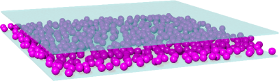
Figure 1: (Color online) A snapshot of our Granular Dynamics simulation for $\phi=0.4$, $\epsilon=0.7$. The Cartesian box dimensions are $L\times L\times 3\sigma$ with $L/\sigma=\sqrt{\pi N/4\phi}\leavevmode\nobreak\ \approx 31.7$.

Figure 1 features a representative snapshot from one of our Granular Dynamics simulations. All simulations are for monodisperse systems of $N=512$ spherical particles with diameter $\sigma$, confined between two horizontal plates at $z=\delta z(x,y)$ and $z=3\sigma+\delta z(x,y)$. Including the gentle sinusoidal surface roughness $\delta z(x,y)=10^{-3}\times\sigma\times\left[\sin(\psi x)+\sin(\psi y)\right]$ with $\psi\sigma=210$ on the plates helps to avoid a suppression of the $x$- and $y$-components of the spheres’ velocities due to friction between the particles and the plates Perera-Burgos et al. (2010). Our choice of the parameter $\psi$ corresponds to a surface roughness wavelength that is much shorter than $\sigma$, resulting in quasi-random lateral velocity kicks.

Periodic boundary conditions are applied in the Cartesian $x$- and $y$-directions, and the particles have three translational and three rotational degrees of freedom. Newton’s equation of motion is integrated in time by means of a Verlet algorithm with a velocity-prediction step Pérez (2008). Forces that act orthogonal to the particle surfaces are modeled by a spring-dashpot model Shäfer et al. (1996), whereas tangential interactions are modeled as Coulomb friction for the sake of simplicity in calculations. The orthogonal forces are characterized by the restitution coefficients $\epsilon$ and $\epsilon_{w}$ in case of particle-particle and particle-wall collisions, respectively. In all our simulations, the particle-wall restitution coefficient $\epsilon_{w}=0.9$ is assumed. For the particle-particle normal restitution coefficient we have used the three values $\epsilon=0.5,0.7$ and $0.9$. The tangential forces in particle pairs and between particles and walls are both characterized by the tangential friction coefficient $\mu=0.4$ in all our simulations.

In an initialization step, the particles are placed at random vertices of a horizontal, two-dimensional triangular lattice with a lattice constant of $1.001\sigma$, at the center plane $z=3\sigma/2$ between the confining plates. All spheres are assigned random velocity vectors $\boldsymbol{v}_{0}$ with magnitudes in the range $0<\left|\boldsymbol{v}_{0}\right|<8\times 10^{-5}\leavevmode\nobreak\ \sigma/\delta t$, and random angular velocity vectors $\boldsymbol{\omega}_{0}$ with magnitudes in the range $0<\left|\boldsymbol{\omega}_{0}\right|<\sqrt{3}\times 10^{-10}\leavevmode\nobreak\ \text{rad}/\delta t$, where $\delta t$ is the time step of the numerical integration scheme. The confining plates are then moved sinusoidally in the $z$-direction with an amplitude $A=0.012678\leavevmode\nobreak\ \sigma$ and a frequency $\nu=1.4\times 10^{-4}/\delta t$. The particles are affected by a gravitational acceleration $g$ in the negative $z$-direction. Setting the value of $g=981\leavevmode\nobreak\ \text{cm}/\text{s}^{2}$, $\sigma=0.5$ cm and $\delta t=2\times 10^{-6}$ s, it is possible to express all simulation parameters in cgs units, so that $\nu=70$ Hz and $A=0.006339$ cm. Such parameters are realistic for experimental systems Bordallo-Favela et al. (2009). The reduced, dimensionless peak acceleration of the plates is $\Gamma=A(2\pi\nu)^{2}/g=1.25$, and we define a quasi-two-dimensional particle packing fraction as $\phi=(\pi N\sigma^{2})/(4L^{2})$, where $L$ is the simulation box length in the $x$- and $y$-directions. We have performed simulations for packing fractions $\phi=0.2,0.4$ and $0.5$.

After a short initial transient, the simulations enter a steady state that appears stationary if short-time averages are considered. In this steady state, the particles rebound vertically and acquire horizontal velocity components due to the surface undulations of the confining plates and also via particle-particle collisions. A snapshot of all particle positions was stored after every 16,667-th time step, corresponding to an interval of $1/30$ s between subsequent recordings. A total number of 2,000 snapshots was recorded for each simulation, with an exception being the system at $\phi=0.2$, $\epsilon=0.5$ (lower right panel in Fig. 5 and Fig. 8) for which we have recorded 10,000 snapshots. From the snapshots we have calculated the projected two-dimensional radial distribution function

$$g_{T}(r)=\dfrac{1}{N}\left\langle\sum\limits_{\begin{subarray}{c}i,j=1\\ i\neq j\end{subarray}}^{N}\delta\left(\boldsymbol{r}^{\parallel}-\boldsymbol{r}^{\parallel}_{i}+\boldsymbol{r}^{\parallel}_{j}\right)\right\rangle$$ (1)

in terms of the Dirac $\delta$ distribution, and the projected two-dimensional static (steady state) structure factor

$$S_{T}(q)=\dfrac{1}{N}\left\langle{\left[\sum\limits_{i=1}^{N}\cos(\boldsymbol{q}^{\parallel}\cdot\boldsymbol{r}^{\parallel}_{i})\right]}^{2}+{\left[\sum\limits_{i=1}^{N}\sin(\boldsymbol{q}^{\parallel}\cdot\boldsymbol{r}^{\parallel}_{i})\right]}^{2}\right\rangle$$ (2)

where $\left\langle\ldots\right\rangle$ stands for the average over all snapshots, $\boldsymbol{r}^{\parallel}_{i}=\left(\mathbb{1}-\hat{\boldsymbol{e}}_{z}\hat{\boldsymbol{e}}_{z}\right)\cdot\boldsymbol{r}_{i}$ is the projection of the position vector $\boldsymbol{r}_{i}$ of particle $i$ into the $(x,y)$-plane, and $\boldsymbol{q}^{\parallel}=\left(\mathbb{1}-\hat{\boldsymbol{e}}_{z}\hat{\boldsymbol{e}}_{z}\right)\cdot\boldsymbol{q}$ is the corresponding projection of the wave vector $\boldsymbol{q}$. The arguments $r=\left|\boldsymbol{r}^{\parallel}\right|$ and $q=\left|\boldsymbol{q}^{\parallel}\right|$ of the correlation functions are the norms of the projected distance and wave vectors. We have checked that all simulated systems are homogeneous and isotropic on average. The lower index ’$T$’ on both functions $g_{T}(r)$ and $S_{T}(q)$ stands for ’Target’, as we have used these functions as the target functions for the Iterative Ornstein–Zernike Inversion method, described in Sec. III.

III Iterative Ornstein–Zernike Inversion

Iterative Ornstein–Zernike Inversion (IO–ZI) is a recently introduced inverse Monte Carlo method that allows to determine the reduced, dimensionless pair potential $\beta u(r)$ of particles in thermodynamic equilibrium from their radial distribution function $g(r)$ and the static structure factor $S(q)$. Here, $\beta=1/(k_{B}T)$ is the inverse thermal energy in terms of the Boltzmann constant $k_{B}$ and the absolute temperature $T$. The interested reader is referred to Ref. Heinen (2018) for a comprehensive description of the IO–ZI method and its validation for three-dimensional fluid systems. For brevity’s sake, we explain here only the essential working principle of IO–ZI, and we mention the differences between the algorithm in Ref. Heinen (2018) and the version for two-dimensional systems that we have used for the present work:

The IO–ZI method shares its underlying principle with the well-established, but less accurate Iterative Boltzmann Inversion (IBI) method Reith et al. (2003). In an initial step, a first estimate $\beta u_{1}(r)$ of the true potential $\beta u(r)$ is calculated via approximate, numerical inversion of the target correlation functions $g_{T}(r)$ and $S_{T}(q)$ at known particle number density $n$. The reduced potential $\beta u_{1}(r)$ is then used in a strictly two-dimensional $(N,V,T)$ Metropolis Monte Carlo (MC) simulation from which the correlation functions $g_{1}(r)$ and $S_{1}(q)$ are extracted. The differences between $g_{T}(r)$ and $g_{1}(r)$ and between $S_{T}(q)$ and $S_{1}(q)$ are the inputs for an iteration update rule by which the function $\beta u_{1}(r)$ is transformed into the next estimate $\beta u_{2}(r)$. The latter serves as the reduced pair potential in a second MC simulation, resulting in $g_{2}(r)$ and $S_{2}(q)$. This sequence of potential adjustments and MC simulations is continued until $g_{n}(r)$ and $S_{n}(q)$ are indistinguishable from $g_{T}(r)$ and $S_{T}(q)$, within the level of the stochastic noise floor. At this point, $\beta u_{n}(r)$ constitutes the output of the IO–ZI (or the IBI) method.

Both the initial seed $\beta u_{1}(r)$ and the iteration update rule in IO–ZI rely on an approximation of the unknown bridge function Hansen and McDonald (1986) in the Ornstein–Zernike integral equation formalism. Different bridge function approximations, also known as closure relations, constitute different flavors of IO–ZI such as Iterative Hypernetted Chain Inversion (IHNCI) which is based on the HNC closure Morita (1958) or Iterative Percus-Yevick Inversion (IPYI), based on the PY closure Percus and Yevick (1958). The IHNCI algorithm has been published in Ref. Heinen (2018), and the IPYI algorithm is obtained if Eqs. (8) and (9) from Ref. Heinen (2018) are replaced by the equations

$$\beta u_{1}(x)=\ln\left[g_{T}(x)-c_{T}(x)\right]-\ln\left[g_{T}(x)\right]$$

and

$$\beta\mu_{i}(x)=\beta u_{i}(x)+\ln\left[\dfrac{g_{T}(x)-c_{T}(x)}{g_{i}(x)-c_{i}(x)}\right]+\ln\left[\dfrac{g_{i}(x)}{g_{T}(x)}\right],$$

respectively. Here, $x=rn^{1/d}$ is the dimensionless particle center-to-center distance in terms of the mean geometric particle distance $n^{-1/d}$. The symbols $\mu_{i}(x)$ and $c_{T}(x)$ denote the output of a single Picard iteration of the IPYI algorithm and the target direct correlation function, respectively. The meaning of both these quantities is discussed in great detail in Ref. Heinen (2018) and will not be repeated here for the sake of brevity.

The IHNCI and IPYI methods are surpassing the IBI method in terms of accuracy of the converged solution for the particle pair potential because the initial seed and the iteration update rule in IBI are both based on the comparatively inaccurate approximation of the true pair potential by the potential of mean force Hansen and McDonald (1986). Moreover, the IO–ZI methods make use of the information contained in the Fourier-space functions $S_{T}(q)$ and $S_{i}(q)$ as well as the real space functions $g_{T}(r)$ and $g_{i}(r)$, whereas the IBI method relies on the real space information from the radial distribution functions only.

The initial seed $\beta u_{1}(r)$ in IHNCI and IPYI is obtained via inversion of the HNC and PY integral equations, respectively. We will therefore use the notation HNC Inversion (HNCI) and PY Inversion (PYI) for the numerical schemes that are obtained when only the initialization steps of IHNCI or IPYI are executed, and the subsequent MC simulations and iterative potential corrections are omitted. The so-obtained PYI method has already been used Bordallo-Favela et al. (2009); Velázquez-Pérez et al. (2016) to calculate effective potentials of granular beads in vibrated quasi-two-dimensional cells, but we are going to demonstrate in Sec. IV that the results from PYI and HNCI are not reliable as they contain a large systematic error. Effective potentials of granular beads that have so far been published must therefore be challenged and re-checked in every particular case.

As an additional technical comment, we note that the necessary inverse Fourier (or Hankel) transform $\mathcal{F}^{-1}$ of the isotropic direct correlation function $\tilde{c}(q)$ from wavenumber space into the real-space function $c(r)$ should preferentially be carried out via the equation

$$c(x)=g(x)-1-\mathcal{F}^{-1}\left\{\dfrac{{\left[S(y)-1\right]}^{2}}{S(y)}\right\}(x)$$

Heinen (2018); Heinen et al. (2011), in which $y=qn^{-1/d}$ is a dimensionless wavenumber, and where the Fourier integrand ${\left[S(y)-1\right]}^{2}/S(y)$ decays considerably quicker as a function of $y$ than the integrand $\tilde{c}(y)$ in $c(x)=\mathcal{F}^{-1}\left\{\tilde{c}(y)\right\}(x)$. A fast decay of the Fourier integrand is a desirable feature as the correlation functions are typically only known in very limited ranges of the variables $x$ and $y$. The Fourier transform is most accurately and conveniently carried out in arbitrary dimension by virtue of Hamilton’s FFTLog algorithm Hamilton (2000); Ham , which is based on Talman’s original publication Talman (1978).

All IHNCI and IPYI runs reported here were carried out with the generalized accelerated fixed-point iteration method originally proposed by Ng Ng (1974); Heinen et al. (2014); Heinen (2018). The MC simulations were performed on a graphics processing unit with ensemble averaging over $256$ statistically independent systems, each containing $256$ particles. While this may appear to be a dangerously small particle number, our results confirm that it is large enough to avoid significant finite size effects on $\beta u(r),g(r)$ and $S(q)$. In the validation and results sections III.1 and IV we will observe that the functions $g(r)$ and $S(q)$ from our ’forward direction’ MC simulations for twice the number of ($N=512$) particles are perfectly reproduced in the inverse MC runs with $N=256$. The physical reason is that the particle interactions are short ranged. Each one of the IHNCI and IPYI runs reported in subsection III.1 and in Sec. IV took $\sim 2$ hours to complete. A HNCI or PYI run requires less than a second of runtime.

III.1 Validation of IO–ZI for two-dimensional systems

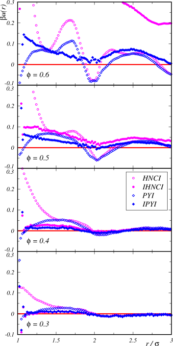
Figure 2: (Color online) The HNCI (open pink circles), IHNCI (filled pink circles), PYI (open blue diamonds) and IPYI (filled blue diamonds) methods are tested in their capabilities to reproduce the pair potential of hard disks in two dimensions (red horizontal lines), at packing fractions $\phi=0.3,0.4,0.5$ and $0.6$ (bottom panel to top panel).

Comprehensive validation tests of the IO–ZI method in its IHNCI flavor have been reported in Ref. Heinen (2018) for systems with various types of particle pair potentials, but in three spatial dimensions only. Before applying IHNCI and IPYI in Sec. IV, we validate both methods for the case of two-dimensional systems in the present subsection.

Figure 2 features the results from the HNCI, IHNCI, PYI and IPYI methods for four test cases in which the target functions $g_{T}(r)$ and $S_{T}(q)$ are those of non-overlapping hard disks in two dimensions, at packing fractions $\phi=0.3,0.4,0.5$ and $0.6$. The functions $g_{T}(r)$ and $S_{T}(q)$ were calculated via Eqs. (1) and (2) in MC simulations of $512$ disks with diameter $\sigma$, in two-dimensional square simulation boxes with periodic boundary conditions in both Cartesian directions. The interaction potential $u(r>\sigma)=0$ is represented by the horizontal red lines in Fig. 2. Any deviation from these lines quantifies an inaccuracy of the HNCI, IHNCI, PYI or IPYI method. Note that IHNCI and IPYI are considerably more accurate than HNCI and PYI in all studied cases, with the exception of the densest system at $\phi=0.6$, where IHNCI fails dramatically. For all other systems at packing fractions $\phi=0.5$ or less, the error of the converged reduced potentials $\beta u(r)$ from IHNCI and IPYI stays below, or well below $0.1$ for practically all particle distances $r$. As one should expect, the IPYI method is more accurate than the IHNCI method (and, likewise, PYI is more accurate than HNCI) in the hard disk test cases. This is due to the well-known fact that the PY closure is more accurate for hard disks than the HNC closure Hansen and McDonald (1986).

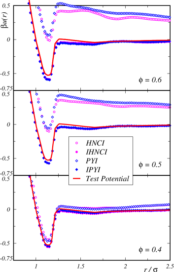
Figure 3: (Color online) Same as Fig. 2, but for a generic freehand-curve test potential (red curves), and at the packing fractions $\phi=0.4,0.5$ and $0.6$ (bottom panel to top panel).

For different interaction potentials, it is in general not known a priori which one of the two closures – HNC or PY – is more accurate. We have therefore conducted a set of three additional validation tests of IHNCI and IPYI with two-dimensional systems at packing fractions $\phi=0.4,0.5$ and $0.6$, where the potential to be reproduced was taken from a digitalized free-hand curve that features strong repulsion at distances $r<\sigma$, an attractive region of maximum depth $-0.5k_{B}T$ in the region $\sigma<r<1.25\sigma$, and a quickly decaying, slightly repulsive part at $r>1.25\sigma$. The results of these tests are shown in Fig. 3, where the red solid curves represent the test potential. The target functions $g_{T}(r)$ and $S_{T}(q)$ for HNCI, IHNCI, PYI and IPYI were extracted from MC simulations of $512$ particles in two-dimensional square simulation boxes with periodic boundary conditions in both Cartesian directions, and with interactions described by the test potential. As a result, we note that IHNCI and IPYI are considerably more accurate in reproducing the test potential than HNCI and PYI, especially at the two higher packing fractions $\phi=0.5$ and $\phi=0.6$.

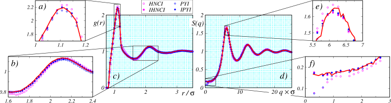
Figure 4: (Color online) Radial distribution functions $g(r)$ and static structure factors $S(q)$ of the systems at packing fraction $\phi=0.5$, and with reduced potentials plotted in the central panel of Fig. 3. Red solid curves represent the target correlation functions $g_{T}(r)$ and $S_{T}(q)$.

The level of accuracy at which the target correlation functions $g_{T}(r)$ and $S_{T}(q)$ are reproduced by the HNCI, IHNCI, PYI and IPYI methods is demonstrated in Fig. 4, which features our results for the systems with reduced potentials plotted in the central panel of Fig. 3: All four inversion methods result in correlation functions $g(r)$ and $S(q)$ that are nearly identical to $g_{T}(r)$ and $S_{T}(q)$, to a level at which the functions are almost indistinguishable within the stochastic noise floor of the simulation results. Nevertheless, close observation of the correlation functions (as in panels a, b, e and f of Fig. 4) reveals that IHNCI is ever so slightly more accurate in reproducing $g_{T}(r)$, $S_{T}(q)$ than HNCI is, and the same can be said about IPYI and its relation to PYI. The minuscule differences between the correlation functions from IHNCI and HNCI, or between IPYI and PYI, are crucial, as they translate into stark differences between the reduced potentials. This is a manifestation of the low practical usefulness of Henderson’s theorem Henderson (1974) as discussed in Refs. Potestio et al. (2014); Heinen (2018): In equilibrium fluids with pairwise additive particle interactions a bijective functional mapping $\beta u(r)\leftrightarrow\left[g(r),S(q)\right]$ is guaranteed to exist, but the mapping is highly nonli near in general. Large differences in $\beta u(r)$ may correspond to tiny differences in $g(r)$ and $S(q)$ which complicates severely the calculation of $\beta u(r)$ from the correlation functions if these are only known within a statistical error margin. This explains the severe failure of simple methods such as HNCI or PYI. More sophisticated methods such as IHNCI, IPYI, or alternative approaches such as pressure-corrected IBI Reith et al. (2003); Potestio et al. (2014) or multistate IBI Moore et al. (2014) are required instead.

A few important characteristics of IHNCI and IPYI can be observed in both Figs. 2 and 3: Both methods are very accurate at small packing fractions and they gradually loose accuracy when the packing fraction is increased. The packing fraction at which any one of the two methods starts to fail gravely can be estimated by comparison with the respective other method. In other words, for cases where IHNCI and IPYI predict similar results, we have strong empirical evidence for the accuracy of both methods. In converse cases where the results of IHNCI and IPYI differ markedly, neither of the two methods can be trusted. We make use of the reassuring comparison between IHNCI and IPYI throughout the results section IV, where the effective potentials for granular particles are calculated by both methods in all cases.

IV Results

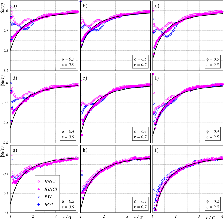
Figure 5: (Color online) Effective potentials for inelastic granular beads at packing fractions $\phi=0.2$ (bottom row of panels), $\phi=0.4$ (central row of panels) and $\phi=0.5$ (top row of panels), and for restitution coefficients $\epsilon=0.9$ (left column of panels), $\epsilon=0.7$ (central column of panels) and $\epsilon=0.5$ (right column of panels). Our results from the HNCI (open pink circles), IHNCI (filled pink circles), PYI (open blue diamonds) and IPYI (filled blue diamonds) methods are shown. One-parametric functions of the form $\alpha/r^{2}$ (black curves) have been fitted to the IHNCI results in the range $1.25<r/\sigma<4$. The horizontal axis range is $1<r/\sigma<4$ is every panel, and the vertical axis range is varying by factors of $2$ from the bottom row to the center row, and from the center row to the top row of panels.

Figure 5 features the main results of the present paper. The HNCI, IHNCI, PYI and IPYI results for the reduced potentials $\beta u(r)$ in nine two-dimensional equilibrium systems are plotted. The input (or target) functions $g_{T}(r)$ and $S_{T}(q)$ for the four inversion methods are those that were obtained from our Granular Dynamics simulations as described in Sec. II, for the restitution coefficients $\epsilon=0.9,0.7$ and $0.5$ and the packing fractions $\phi=0.2,0.4$ and $0.5$. We have also conducted Granular Dynamics simulations at $\phi=0.6$ but we refrain from showing the results for the effective potentials here, as each one of the four inversion methods is clearly failing at $\phi=0.6$. Our observations in Fig. 5 are the following:

The HNCI and PYI results are in strong disagreement with each other and with the IHNCI and IPYI results, for all but the most dilute systems at $\phi=0.2$ (panels g, h and i of Fig. 5). Both HNCI and PYI are thus unreliable and should never be used in the determination of effective interaction potentials.

Our PYI results for $\beta u(r)$ at $\phi=0.4$ (panels d, e and f of Fig. 5) resemble those in Fig. 4 of Ref. Velázquez-Pérez et al. (2016) as far as the shape of the functions is concerned, but the reduced potentials in Ref. Velázquez-Pérez et al. (2016) are more strongly attractive, with a minimum value around $-1$ to $-1.5$, which is approximately three times deeper than the minima of our results for $\beta u(r)$ at $\phi=0.4$. We presume that the reason for this quantitative disagreement might be a difference between the particle-wall restitution coefficients $\epsilon_{w}$ of our Granular Dynamics simulations and those that were used in Ref. Velázquez-Pérez et al. (2016). If the value of $\epsilon_{w}$ was chosen smaller than our value of $\epsilon_{w}=0.9$, then the effective, kinetic temperature of the Granular beads in Ref. Velázquez-Pérez et al. (2016) can be expected to be lower than in our case, which would be in line with a larger value of $\beta$. Unfortunately we are not in the position to test our presumption as the value of $\epsilon_{w}$ has not been reported in Ref. Velázquez-Pérez et al. (2016).

Our IHNCI and IPYI results are in close agreement with each other, in all nine cases shown in Fig. 5, which serves as a reassurance for the fidelity of both methods. A non-trivial finding is that both IHNCI and IPYI are converging in all nine cases, and that the target correlation functions $g_{T}(r)$ and $S_{T}(q)$ of the out-of-equilibrium granular systems are reproduced by the two methods (as we have checked in every case). This implies that there is indeed an equilibrium system with correlation functions identical to those of the granular system in the entire parameter range $0.2\leq\phi\leq 0.5$ and $0.5\leq\epsilon\leq 0.9$.

The effective potentials from IHNCI and IPYI are attractive and follow a simple, monotonically increasing and concave shape in all cases, with the exception of the system at $\phi=0.2$ and $\epsilon=0.9$ in panel g of Fig. 5, where a gentle upturn of the reduced potentials is observed at very close particle proximity. We cannot be sure about the statistical significance of that upturn and refrain from over-interpreting it as a physical effect as it may just as well be a numerical artifact. That the effective interactions are attractive is physically quite intuitive: In a steady state with vanishing average particle currents, the normal velocity restitution causes an increase in particle number density around any tagged particle, as it is also caused by attractive interactions in the effective equilibrium system with the same particle correlation functions.

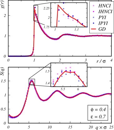
Figure 6: (Color online) Radial distribution function (upper panel) and structure factor (lower panel) for $\phi=0.4$ and $\epsilon=0.7$. Solid red curves are our Granular Dynamics (GD) results, extracted from the simulations via Eqs. (1) and (2). The corresponding effective potentials are plotted in the central panel of Fig. 5.

The correlation functions for the system at $\phi=0.4$, $\epsilon=0.7$ (central panel ‘e’ in Fig. 5, also featured in Fig. 1) are shown in Fig. 6, where an upturn of $S(q)$ at small values of $q$ supports our finding of attractive effective interactions, and $g(r<\sigma)\ll 1$ signals that the granular system is indeed nearly perfectly two-dimensional.

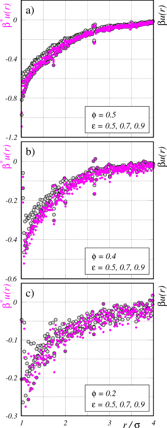
Figure 7: (Color online) Black circles filled in gray: Converged IHNCI potentials from Fig. 7. Pink circles: The same data, rescaled with respect to the effective granular temperature and the effective inverse thermal energy $\beta^{*}$, as described in the main text. Every panel is for one packing fraction $\phi$. The results for different restitution coefficients $\epsilon$, corresponding to different values of $\beta^{*}$, are overlaid in the panels. The vertical spread among the data narrows upon effective temperature rescaling.

Figure 7 repeats all the converged IHNCI potentials from Fig. 5 as black circles filled in gray. Every panel of Fig. 7 is for one of the three packing fractions $\phi=0.2,0.4$ and $0.5$, as indicated in the panels a – c. The panels contain the results for three different restitution coefficients $\epsilon=0.5,0.7$ and $0.9$ in an overlaid manner, such that the spread among the symbols of equal type indicates the difference between the results for equal packing fraction and for varying coefficient of restitution. While the data for different $\epsilon$ appear to follow the same functional form (within statistical scatter), the observed vertical spread among the black/gray circles indicates that different values of $\epsilon$ correspond to different values of the effective inverse thermal energy $\beta$. Keeping in mind that all our data are for equal intensities of vertical shaking, this apparent spread in effective granular temperature is in line with the intuitive picture in which different restitution coefficients $\epsilon$ correspond to different amounts of kinetic energy dissipation in the steady state.

As wee have checked, the distributions of the Cartesian velocity components parallel to the confining plates are nearly Maxwellian, with slight deviations from the Maxwellian form for very slow and very fast velocities. This is in line with the observations that have been reported in several instances in the literature Olafsen and Urbach (1999); van Zon et al. (2004).

An effective granular temperature was determined for each of the cases displayed in Figs. 5, 7, by fitting the Cartesian velocity histograms from our Granular Dynamics simulations to Maxwellian (Gaussian) functions, using the variance $\sigma(\phi,\epsilon)$ of the distribution for each given pair of values $(\phi,\epsilon)$ as a fit parameter. Assuming that the so-determined velocity variance is proportional to an effective granular Temperature, we have rescaled the data with prefactors $\beta^{*}(\phi,\epsilon)=\beta(\phi,\epsilon)\times\sigma(\phi,\epsilon)/\sigma(\phi,\epsilon=0.5)$. That is: we have scaled all data for equal $\phi$ and different $\epsilon$ to the effective granular temperature that corresponds to $\epsilon=0.5$. The results can be observed in Fig. 7 as the pink symbols, the spread among which is considerably less than the spread among the black/gray symbols, especially for the two higher packing fractions $\phi=0.4$ and $0.5$ (panels b and a of Fig. 7, respectively). This confirms that $\sigma(\phi,\epsilon)$ is a good measure for an effective granular temperature. It also supports the conceptual idea of fitting the out-of-equilibrium, steady state particle pair correlations with those of equilibrium systems, as it is done in the IO–ZI methods.

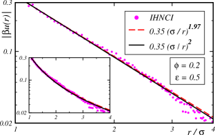
Figure 8: (Color online) Circles: Absolute value of the reduced effective IHNCI potential for $\phi=0.2$, $\epsilon=0.5$ (as in panel i of Fig. 5) on a double logarithmic and a linear-logarithmic scale (inset). Red dashed curve: Two-parametric fit in which both the prefactor and the exponent were allowed to vary. Black solid curve: One-parametric fit with fixed exponent of $-2$, where only the prefactor was adjusted.

The observed simple shapes of $\beta u(r)$ in Fig. 5 encourage an attempt to determine the functional form of the potential, at least for the most dilute case $\phi=0.2$. To this end, in Fig. 8 we are plotting the absolute value of $\beta u(r)$ from IHNCI, for $\phi=0.2$, $\epsilon=0.5$ (as in panel i of Fig. 5) on a double logarithmic scale and on a linear-logarithmic scale (inset of Fig. 8). An exponential form of the potential is ruled out by the linear-logarithmic plot, where the IHNCI results exhibit a significant non-zero curvature. The double logarithmic plot reveals that the IHNCI result is compatible with the power law $\beta u(r)=\alpha\leavevmode\nobreak\ r^{-2}$, with a single adjustable parameter $\alpha$. If the exponent in the power law is allowed to vary in a non-linear regression-like fit, then an optimal exponent of $-1.97$ is obtained, providing strong support for the hypothesized exponent of $-2$. In default of an analytical theory for the shape of the potential, we do not want to over-interpret the results in Fig. 8 by stating that the effective potential is truly of the form $\beta u(r)=\alpha\leavevmode\nobreak\ r^{-2}$. We merely report that our data is compatible with such a power law, and that the theoretical justification or falsification of the power law is a rewarding task for future studies.

V Conclusions

Our successful application of IO–ZI in its two flavors IHNCI and IPYI demonstrates that the particle correlation functions in quasi-two-dimensional vibrated granular systems can be mapped onto those of an equivalent, truly equilibrium system in a wide range of granular packing fractions and restitution coefficients. The resulting effective interaction potentials exhibit a simple shape that is in line with intuitive physical arguments. At low packing fraction, there is strong empirical evidence for the one-parametric power-law form $\beta u(r)=\alpha\leavevmode\nobreak\ r^{-2}$ of the effective potential. Additional analytical-theoretical work is required to support or falsify the validity of the suggested power-law form of $\beta u(r)$. The simple HNCI and PYI methods should not be used in the determination of (effective) particle interaction potentials as the results of these methods suffer from great systematic errors unless the particle packing fraction is very small. Our work includes the first reported validation of IHNCI and IPYI for two-dimensional systems. Both methods are awaiting further applications in two- and three-dimensional granular, molecular and Brownian systems.

References

- Aranson and Tsimring (2006) I. S. Aranson and L. S. Tsimring, Rev. Mod. Phys. 78, 641 (2006).
- van der Meer et al. (2002) D. van der Meer, K. van der Weele, and D. Lohse, Phys. Rev. Lett. 88, 174302 (2002).
- Sanders et al. (2004) D. A. Sanders, M. R. Swift, R. M. Bowley, and P. J. King, Phys. Rev. Lett. 93, 208002 (2004).
- Rosato et al. (1987) A. Rosato, K. J. Strandburg, F. Prinz, and R. H. Swendsen, Phys. Rev. Lett. 58, 1038 (1987).
- Olafsen and Urbach (1998) J. S. Olafsen and J. S. Urbach, Phys. Rev. Lett. 81, 4369 (1998).
- Roeller et al. (2011) K. Roeller, J. P. D. Clewett, R. M. Bowley, S. Herminghaus, and M. R. Swift, Phys. Rev. Lett. 107, 048002 (2011).
- Prevost et al. (2004) A. Prevost, P. Melby, D. A. Egolf, and J. S. Urbach, Phys. Rev. E 70, 050301 (2004).
- Risso et al. (2018) D. Risso, R. Soto, and M. Guzmán, Phys. Rev. E 98, 022901 (2018).
- Goldhirsch and Zanetti (1993) I. Goldhirsch and G. Zanetti, Phys. Rev. Lett. 70, 1619 (1993).
- Ciamarra et al. (2006) M. P. Ciamarra, A. Coniglio, and M. Nicodemi, Phys. Rev. Lett. 97, 038001 (2006).
- Bordallo-Favela et al. (2009) R. A. Bordallo-Favela, A. Ramírez-Saíto, C. A. Pacheco-Molina, J. A. Perera-Burgos, Y. Nahmad-Molinari, and G. Pérez, Eur. Phys. J. E 28, 395 (2009).
- Tapia-Ignacio et al. (2016) C. Tapia-Ignacio, J. Garcia-Serrano, and F. Donado, Phys. Rev. E 94, 062902 (2016).
- Donado et al. (2017) F. Donado, J. M. Sausedo-Solorio, and R. E. Moctezuma, Phys. Rev. E 95, 022601 (2017).
- Percus and Yevick (1958) J. K. Percus and G. J. Yevick, Phys. Rev. 110, 1 (1958).
- Velázquez-Pérez et al. (2016) S. Velázquez-Pérez, G. Pérez-Ángel, and Y. Nahmad-Molinari, Phys. Rev. E 94, 032903 (2016).
- Heinen (2018) M. Heinen, J. Comput. Chem. (2018), 10.1002/jcc.25225.
- Perera-Burgos et al. (2010) J. A. Perera-Burgos, G. Pérez-Ángel, and Y. Nahmad-Molinari, Physical Review E 82, 051305 (2010).
- Pérez (2008) G. Pérez, PRAMANA-journal of physics 70, 989 (2008).
- Shäfer et al. (1996) J. Shäfer, S. Dippel, and D. Wolf, Journal de physique I 6, 5 (1996).
- Reith et al. (2003) D. Reith, M. Pütz, and F. Müller-Plathe, J. Comput. Chem. 24, 1624 (2003).
- Hansen and McDonald (1986) J.-P. Hansen and I. R. McDonald, Theory of Simple Liquids, 3rd ed. (Academic Press, London, 1986).
- Morita (1958) T. Morita, Prog. Theo. Phys. 20, 920 (1958).
- Heinen et al. (2011) M. Heinen, P. Holmqvist, A. J. Banchio, and G. Nägele, J. Chem. Phys. 134, 044532, ibid. 129901 (2011).
- Hamilton (2000) A. J. S. Hamilton, Mon. Not. R. Astron. Soc. 312, 257 (2000).
- (25) http://casa.colorado.edu/~ajsh/FFTLog/.
- Talman (1978) J. D. Talman, J. Comput. Phys. 29, 35 (1978).
- Ng (1974) K.-C. Ng, J. Chem. Phys. 61, 2680 (1974).
- Heinen et al. (2014) M. Heinen, E. Allahyarov, and H. Löwen, J. Comput. Chem. 35, 275 (2014).
- Henderson (1974) R. L. Henderson, Phys. Lett. A49, 197 (1974).
- Potestio et al. (2014) R. Potestio, C. Peter, and K. Kremer, Entropy 16, 4199 (2014).
- Moore et al. (2014) T. C. Moore, C. R. Iacovella, and C. McCabe, J. Chem. Phys. 140, 224104 (2014).
- Olafsen and Urbach (1999) J. S. Olafsen and J. S. Urbach, Phys. Rev. E 60, R2468 (1999).
- van Zon et al. (2004) J. S. van Zon, J. Kreft, D. I. Goldman, D. Miracle, J. B. Swift, and H. L. Swinney, Phys. Rev. E 70, 040301 (2004).