Optimizing weighted ensemble sampling of steady states

Abstract

We propose parameter optimization techniques for weighted ensemble sampling of Markov chains in the steady-state regime. Weighted ensemble consists of replicas of a Markov chain, each carrying a weight, that are periodically resampled according to their weights inside of each of a number of bins that partition state space. We derive, from first principles, strategies for optimizing the choices of weighted ensemble parameters, in particular the choice of bins and the number of replicas to maintain in each bin. In a simple numerical example, we compare our new strategies with more traditional ones and with direct Monte Carlo.

65C05, 65C20, 65C40, 65Y05, 82C80

1 Introduction

Weighted ensemble is a Monte Carlo method based on stratification and resampling, originally designed to solve problems in computational chemistry [8, 12, 15, 17, 18, 23, 34, 46, 47, 51, 62, 63, 65, 67]. Weighted ensemble currently has a substantial user base; see [66] for software and a more complete list of publications. In general terms, the method consists of periodically resampling from an ensemble of weighted replicas of a Markov process. In each of a number of bins, a certain number of replicas is maintained according to a prescribed replica allocation. The weights are adjusted so that the weighted ensemble has the correct distribution [63]. In the context of rare event or small probability calculations, weighted ensemble can significantly outperform direct Monte Carlo, or independent replicas; the performance gain comes from allocating more particles to important or rare regions of state space. In this sense, weighted ensemble can be understood as an importance sampling method. We assume the underlying Markov process is expensive to simulate, so that optimizing variance versus cost is critical. In applications, the Markov process is usually a high dimensional drift diffusion, such as Langevin molecular dynamics [50], or a continuous time Markov chain representing reaction network dynamics [3].

We focus on the computation of the average of a given function or observable with respect to the unique steady state of the Markov process, though many of our ideas could also be applied in a finite time setting. One of the most common applications of weighted ensemble is the computation of a mean first passage time, or the mean time for a Markov process to go from an initial state to some target set. The mean first passage time is an important quantity in physical and chemical processes, but it can be prohibitively large to compute using direct Monte Carlo simulation [1, 33, 42]. In weighted ensemble, the mean first passage time to a target set is reformulated, via the Hill relation [32], as the inverse of the steady state flux into the target. Here, the observable is the characteristic or indicator function of the target set, and the flux is the steady-state average of this observable. This steady state can sometimes be accessed on time scales much smaller than the mean first passage time [1, 16, 64]. On the other hand, when the mean first passage time is very large, the corresponding steady state flux is very small and needs to be estimated with substantial precision, which is why importance sampling is needed. The steady state in this case, and in most weighted ensemble applications, is not known up to a normalization factor. As a result, many standard Monte Carlo methods, including those based on Metropolis-Hastings, do not apply.

In this article we consider weighted ensemble parameter optimization for steady state averages. Our work here expands on related results in [5] for weighted ensemble optimization on finite time horizons. For a given Markov chain, weighted ensemble is completely characterized by the choice of resampling times, bins, and replica allocation. In this article we discuss how to choose the bins and replica allocation. We also argue that the frequency of resampling times is mainly limited by processor interaction cost and not variance. We use a first-principles, finite replica analysis based on Doob decomposing the weighted ensemble variance. Our earlier work [5] is based on this same mathematical technique, but the methods described there are not suitable for long-time computations or bin optimization [4]. As is usual in importance sampling, our parameter optimizations require estimates of the very variance terms we want to minimize. However, because weighted ensemble is statistically exact no matter the parameters [4, 63], these estimates can be crude. The choice of parameters affects the variance, not the mean; we only require parameters that are good enough to beat direct Monte Carlo.

From the point of view of applications, similar particle methods employing stratification include Exact Milestoning [7], Non-Equilibrium Umbrella Sampling [56, 22], Transition Interface Sampling [53], Trajectory Tilting [54], and Boxed Molecular dynamics [30]. There are related methods based on sampling reactive paths, or paths going directly from a source to a target, in the context of the mean first passage time problem just cited. Such methods include Forward Flux Sampling [2] and Adaptive Multilevel Splitting [9, 10, 11]. These methods differ from weighted ensemble in that they estimate the mean first passage time directly from reactive paths rather than from steady state and the Hill relation. In contrast with many of these methods, weighted ensemble is simple enough to allow for a relatively straightforward non-asymptotic variance analysis based on Doob decomposition [24].

From a mathematical viewpoint, weighted ensemble is simply a resampling-based evolutionary algorithm. In this sense it resembles particle filters, sequential importance sampling, and sequential Monte Carlo. For a review of sequential Monte Carlo, see the textbook [19], the articles [20, 21] or the compilation [28]. There is some recent work on optimizing the Gibbs-Boltzmann input potential functions in sequential Monte Carlo [6, 13, 36, 57, 61] (see also [21]). We emphasize that weighted ensemble is different from most sequential Monte Carlo methods, as it relies on a bin-based resampling mechanism rather than a globally defined fitness function like a Gibbs-Boltzmann potential. In particular, sequential Monte Carlo is more commonly used to sample rare events on finite time horizons, and may not be appropriate for very long time computations of the sort considered here, as explained in [4].

To our knowledge, the binning and particle allocation strategies we derive here are new. A similar allocation strategy for weighted ensemble on finite time horizons was proposed in [5]. Our allocation strategy, which minimizes mutation variance – the variance corresponding to evolution of the replicas – extends ideas from [5] to our steady-state setup. We draw an analogy between minimizing mutation variance and minimizing sensitivity in an Appendix. In most weighted ensemble simulations, and in [5], bins are chosen in an ad hoc way. We show below, however, that choosing bins carefully is important, particularly if relatively few can be afforded. We propose a new binning strategy based on minimizing selection variance – the variance associated with resampling from the replicas – in which weighted ensemble bins are aggregated from a collection of smaller microbins [15].

Formulas for the mutation and selection variance are derived in a companion paper [4] that proves an ergodic theorem for weighted ensemble time averages. These variance formulas, which we use to define our allocation and bin optimizations, involve the Markov kernel $K$ that describes the evolution of the underlying Markov process between resampling times, as well as the solution, $h$, of a certain Poisson equation. We propose estimating $K$ and $h$ with techniques from Markov state modeling [35, 45, 48, 49]. In this formulation, the microbins correspond to the Markov states, and a microbin-to-microbin transition matrix defines the approximations of $K$ and $h$.

This article is organized as follows. In Section 2, we introduce notation, give an overview of weighted ensemble, and describe the parameters we wish to optimize. In Section 3, we present weighted ensemble in precise detail (Algorithm 1), reproduce the aforementioned variance formulas (Lemmas 3.4 and 3.5) from our companion paper [4], and describe the solution, $h$, to a certain Poisson equation arising from these formulas (equations (15) and (16)). In Section 4, we introduce novel optimization problems (equations (LABEL:opt_allocation) and (LABEL:opt_bins)) for choosing the bins and particle allocation. The resulting allocation in (20) can be seen as a version of equation (6.4) in [5], modified for steady state and our new microbin setup. These optimizations are idealized in the sense that they involve $K$ and $h$, which cannot be computed exactly. Thus in Section 5, we propose using microbins and Markov state modeling to estimate their solutions (Algorithms 2 and 27). In Section 6, we test our methods with a simple numerical example (Figures 1-4). Concluding remarks and suggestions for future work are in Section 7. In the Appendix, we describe residual resampling [26], a common resampling technique, and draw an analogy between sensitivity and our mutation variance minimization strategy.

2 Algorithm

A weighted ensemble consists of a collection of replicas, or particles, belonging to a common state space, with associated positive scalar weights. The particles repeatedly undergo resampling and evolution steps. Using a genealogical analogy, we refer to particles before resampling as parents, and just after resampling as children. A child is initially just a copy of its parent, though it evolves independently of other children of the same parent. The total weight remains constant in time, which is important for the stability of long-time averages [4] (and is a critical difference between the optimization algorithm described in [5] and the one outlined here). Between resampling steps, the particles evolve independently via the same Markov kernel $K$. The initial parents can be arbitrary, though their weights must sum to $1$; see Algorithm 4 for a description of an initialization step tailored to steady-state calculations. The number $N_{\textup{init}}$ of initial particles can be larger than the number $N$ of weighted ensemble particles after the first resampling step.

For the resampling or selection step, we require a collection of bins, denoted ${\mathcal{B}}$, and a particle allocation $N_{t}(u)_{t\geq 0}^{u\in{\mathcal{B}}}$, where $N_{t}(u)$ is the (nonnegative integer) number of children in bin $u\in{\mathcal{B}}$ at time $t$. We will assume the bins form a partition of state space (though in general they can be any grouping of the particles [4]). The total number of children is always $N=\sum_{u\in{\mathcal{B}}}N_{t}(u)$. Both the bins and particle allocation are user-chosen parameters, and to a large extent this article concerns how to pick these parameters. In general, the bins and particle allocation can be time dependent and adaptive. For simpler presentation, however, we assume that the bins are based on a fixed partition of state space. After selection, the weight of each child in bin $u\in{\mathcal{B}}$ is $\omega_{t}(u)/N_{t}(u)$, where $\omega_{t}(u)$ is the sum of the weights of all the parents in bin $u$. By construction, this preserves the total weight $\sum_{u\in{\mathcal{B}}}\omega_{t}(u)=1$. In every occupied bin $u$, the $N_{t}(u)\geq 1$ children are selected from the parents in bin $u$ with probability proportional to the parents’ weights. (Here, we mean bin $u$ is occupied if $\omega_{t}(u)>0$. In unoccupied bins, where $\omega_{t}(u)=0$, we set $N_{t}(u)=0$.)

In the evolution or mutation step, the time $t$ advances, and all the children independently evolve one step according to a fixed Markov kernel $K$, keeping their weights from the selection step, and becoming the next parents. In practice, $K$ corresponds to the underlying process evaluated at resampling times $\Delta t$. That is, $K$ is a $\Delta t$-skeleton of the underlying Markov process [43]. For the mathematical analysis below, this will only be important when we consider varying the resampling times, and in particular the $\Delta t\to 0$ limit. (We think of this underlying process as being continuous in time, though of course time discretization is usually required for simulations. Weighted ensemble is used on top of an integrator of the underlying process; in particular weighted ensemble does not handle the time discretization. We will not be concerned with the unavoidable error resulting from time discretization.) We assume that $K$ is uniformly geometrically ergodic [27] with respect to a stationary distribution, or steady state, $\mu$. Recall we are interested in steady-state averages. Thus for a given bounded real-valued function or observable $f$ on state space, we estimate $\int f\,d\mu$ at each time by evaluating the weighted sum of $f$ on the current collection of parent particles.

We summarize weighted ensemble as follows:

• In the selection step at time $t$, inside each bin $u$, we resample $N_{t}(u)$ children from the parents in $u$, according to the distribution defined by their weights. After selection, all the children in bin $u$ have the same weight $\omega_{t}(u)/N_{t}(u)$, where $\omega_{t}(u)$ is the total weight in bin $u$ before and after selection.

• In each mutation step, the children evolve independently according to the Markov kernel $K$. After evolution, these children become the new parents.

• The weighted ensemble evolves by repeated selection and then mutation steps. The time $t$ advances after a single pair of selection and mutation steps.

See Algorithm 1 for a detailed description of weighted ensemble.

An important property of weighted ensemble is that it is unbiased no matter the choice of parameters: at time $t$ the weighted particles have the same distribution as a Markov chain evolving according to $K$. See Theorem 3.1. With bad parameters, however, weighted ensemble can suffer from large variance, even worse than direct Monte Carlo. As there is no free lunch, choosing parameters cleverly requires either some information about $K$, perhaps gleaned from prior simulations or obtained adaptively during weighted ensemble simulations. We will assume we have a collection of microbins which we use to gain information about $K$. The microbins, like the weighted ensemble bins, form a partition of state space, and each bin will be a union of microbins. We use the term microbins because the microbins may be smaller than the actual weighted ensemble bins. We discuss the reasoning behind this distinction in Section 5; see Remark 5.1.

3 Mathematical notation and algorithm

We write $\xi_{t}^{1},\ldots,\xi_{t}^{N}$ for the parents at time $t$ and $\omega_{t}^{1},\ldots,\omega_{t}^{N}$ for their weights. Their children are denoted $\hat{\xi}_{t}^{1},\ldots,\hat{\xi}_{t}^{N}$ with weights $\hat{\omega}_{t}^{1},\ldots,\hat{\omega}_{t}^{N}$. Thus, weighted ensemble advances in time as follows:

$$\{\xi_{t}^{i}\}^{i=1,\ldots,N}\xrightarrow{\textup{selection}}\{{\hat{\xi}}_{t}^{i}\}^{i=1,\ldots,N}\xrightarrow{\textup{mutation}}\{{\xi}_{t+1}^{i}\}^{i=1,\ldots,N},$$

$$\{\omega_{t}^{i}\}^{i=1,\ldots,N}\xrightarrow{\textup{selection}}\{{\hat{\omega}}_{t}^{i}\}^{i=1,\ldots,{N}}\xrightarrow{\textup{mutation}}\{{\omega}_{t+1}^{i}\}^{i=1,\ldots,N}.$$

The particles belong a common standard Borel state space [29]. This state space is divided into a finite collection ${\mathcal{B}}$ of disjoint subsets (throughout we only consider measurable sets and functions). We define the bin weights at time $t$ as

$$\omega_{t}(u)=\sum_{i:\xi_{t}^{i}\in u}\omega_{t}^{i},\qquad u\in{\mathcal{B}},$$

where the empty sum is zero (so an unoccupied bin $u$ has $\omega_{t}(u)=0$).

For the parent $\xi_{t}^{i}$ of $\hat{\xi}_{t}^{j}$, we write $\text{par}(\hat{\xi}_{t}^{j})=\xi_{t}^{i}$. A child is just a copy of its parent:

$$\text{par}(\hat{\xi}_{t}^{j})=\xi_{t}^{i}\text{ implies }\hat{\xi}_{t}^{j}=\xi_{t}^{i}.$$

Each child has a unique parent. Setting the number of children of each parent completely defines the children, as the choices of the children’s indices (the $j$’s in $\hat{\xi}_{t}^{j}$) do not matter. The number of children of $\xi_{t}^{i}$ will be written $C_{t}^{i}$:

(1) $$C_{t}^{i}=\#\{j:\textup{par}(\hat{\xi}_{t}^{j})=\xi_{t}^{i}\},$$

where $\#S=$ number of elements in a set $S$.

Recall that $N_{t}(u)$ is the number of children in bin $u$ at time $t$. We require that there is at least one child in each occupied bin, no children in unoccupied bins, and $N$ total children at each time $t$. Thus,

(2) $$N_{t}(u)\geq 1\text{ if }\omega_{t}(u)>0,\qquad N_{t}(u)=0\text{ if }\omega_{t}(u)=0,\qquad\sum_{u\in{\mathcal{B}}}N_{t}(u)=N.$$

We write ${\mathcal{F}}_{t}$ for the $\sigma$-algebra generated by the weighted ensemble up to, but not including, the $t$-th selection step. We will assume the particle allocation is known before selection. Similarly, we write $\hat{\mathcal{F}}_{t}$ for the $\sigma$-algebra generated by weighted ensemble up to and including the $t$-th selection step. In detail,

$${\mathcal{F}}_{t} =\sigma\left((\xi_{s}^{i},\omega_{s}^{i})_{0\leq s\leq t}^{i=1,\ldots,N},N_{s}(u)_{0\leq s\leq t}^{u\in{\mathcal{B}}},(\hat{\xi}_{s}^{i},\hat{\omega}_{s}^{i})_{0\leq s\leq t-1}^{i=1,\ldots,N},(C_{s}^{i})_{0\leq s\leq t-1}^{i=1,\ldots,N}\right)$$

$$\hat{\mathcal{F}}_{t} =\sigma\left((\xi_{s}^{i},\omega_{s}^{i})_{0\leq s\leq t}^{i=1,\ldots,N},N_{s}(u)_{0\leq s\leq t}^{u\in{\mathcal{B}}},(\hat{\xi}_{s}^{i},\hat{\omega}_{s}^{i})_{0\leq s\leq t}^{i=1,\ldots,N},(C_{s}^{i})_{0\leq s\leq t}^{i=1,\ldots,N}\right).$$

Algorithm 1 Weighted ensemble

Pick initial parents and weights $(\xi_{0}^{i},\omega_{0}^{i})^{i=1,\ldots,N_{\textup{init}}}$ with $\sum_{i=1}^{N_{\textup{init}}}\omega_{0}^{i}=1$, choose a collection ${\mathcal{B}}$ of bins, and define a final time $T$. Then for $t\geq 0$, iterate the following:

• (Selection step) Each parent $\xi_{t}^{i}$ is assigned a number $C_{t}^{i}$ of children, as follows:

  In each occupied bin $u\in{\mathcal{B}}$, conditional on ${\mathcal{F}}_{t}$, let $(C_{t}^{i})^{i:\textup{bin}(\xi_{t}^{i})=u}$ be $N_{t}(u)$ samples from the distribution $\{\omega_{t}^{i}/\omega_{t}(u):\,\xi_{t}^{i}\in u\}$, where $N_{t}(u)^{u\in{\mathcal{B}}}$ satisfies (2). The children $(\hat{\xi}_{t}^{i})^{i=1,\ldots,N}$ are defined by (1), with weights

  (3) $${\hat{\omega}}_{t}^{i}=\frac{\omega_{t}(u)}{N_{t}(u)},\qquad\textup{if }{\hat{\xi}}_{t}^{i}\in u.$$

  Selections in distinct bins are conditionally independent.

• (Mutation step) Each child $\hat{\xi}_{t}^{i}$ independently evolves one time step. Thus: Conditionally on $\hat{\mathcal{F}}_{t}$, the children $(\hat{\xi}_{t}^{i})^{i=1,\ldots,N}$ evolve independently according to the Markov kernel $K$, becoming the next parents $({\xi}_{t+1}^{i})^{i=1,\ldots,N}$, with weights

  (4) $$\omega_{t+1}^{i}={\hat{\omega}}_{t}^{i},\qquad i=1,\ldots,N.$$

  Then time advances, $t\leftarrow t+1$. Stop if $t=T$, else return to the selection step.

Algorithm 2 outlines an optimization for the allocation $N_{t}(u)^{u\in{\mathcal{B}}}$, and a procedure for choosing the bins ${\mathcal{B}}$ is in Algorithm 27. For the initialization, see Algorithm 4.

In Algorithm 1, we do not explicitly say how we sample the $N_{t}(u)$ children in each bin $u$. Our framework below allows for any unbiased resampling scheme. We give a selection variance formula that assumes residual resampling; see Lemma 3.5 and Algorithm 5. Residual resampling has performance on par with other standard resampling methods like systematic and stratified resampling [26]. See [58] for more details on resampling in the context of sequential Monte Carlo.

3.1 Ergodic averages

We are interested in using Algorithm 1 to estimate

$$\theta_{T}\approx\int f\,d\mu$$

where we recall $\mu$ is the stationary distribution of the Markov kernel $K$, and

(5) $$\theta_{T}=\frac{1}{T}\sum_{t=0}^{T-1}\sum_{i=1}^{N}\omega_{t}^{i}f(\xi_{t}^{i}).$$

Note that $\theta_{T}$ is simply the running average of $f$ over the weighted ensemble up to time $T-1$. In particular, (5) is not a time average over ancestral lines that survive up to time $T-1$, but rather it is an average over the weighted ensemble at each time $0\leq t\leq T-1$. Our time averages (5) require no replica storage and should have smaller variances than averages over surviving ancestral lines [4].

3.2 Consistency results

The next results, from a companion article [4], show that weighted ensemble is unbiased and that weighted ensemble time averages converge. The latter does not in general follow from the former, as standard unbiased particle methods such as sequential Monte Carlo can have variance explosion [4]. (The proofs in [4] have $N_{\textup{init}}=N$, but they are easily modified for $N_{\textup{init}}\neq N$.)

Theorem 3.1 (From [4]).

In Algorithm 1, suppose that the initial particles and weights are distributed as $\nu$, in the sense that

(6) $${\mathbb{E}}\left[\sum_{i=1}^{N_{\textup{init}}}\omega_{0}^{i}g(\xi_{0}^{i})\right]=\int g\,d\nu$$

for all real-valued bounded functions $g$ on state space. Let $(\xi_{t})_{t\geq 0}$ be a Markov chain with kernel $K$ and initial distribution $\xi_{0}\sim\nu$. Then for any time $T>0$,

$${\mathbb{E}}\left[\sum_{i=1}^{N}\omega_{T}^{i}g(\xi_{T}^{i})\right]={\mathbb{E}}[g(\xi_{T})]$$

for all real-valued bounded functions $g$ on state space.

Recall we assume $K$ is uniformly geometrically ergodic [27].

Theorem 3.2 (From [4]).

Weighted ensemble is ergodic in the following sense:

$$\lim_{T\to\infty}\theta_{T}\stackrel{{\scriptstyle a.s.}}{{=}}\int f\,d\mu.$$

Theorem 3.1 does not use ergodicity of $K$, though Theorem 3.2 obviously does.

3.3 Variance analysis

We will make use of the following analysis from [4] concerning the weighted ensemble variance. Define the Doob martingales [25]

(7) $$D_{t}={\mathbb{E}}[\theta_{T}|{\mathcal{F}}_{t}],\qquad\hat{D}_{t}={\mathbb{E}}[\theta_{T}|\hat{\mathcal{F}}_{t}].$$

The Doob decomposition in Theorem 3.3 below filters the variance through the $\sigma$-algebras ${\mathcal{F}}_{t}$ and $\hat{\mathcal{F}}_{t}$. It is a way to decompose the variance into contributions from the initial condition and each time step. This type of telescopic variance decomposition is standard in sequential Monte Carlo, although it is usually applied at the level of measures on state space, which corresponds to the infinite particle limit $N\to\infty$ [19]. We use the finite $N$ formula directly to minimize variance, building on ideas in [5].

Theorem 3.3 (From [4]).

By Doob decomposition,

(8) $$\theta_{T}^{2}-{\mathbb{E}}[\theta_{T}]^{2}+R_{T} =\left(D_{0}-{\mathbb{E}}[\theta_{T}]\right)^{2}$$

(9) $$\quad+\sum_{t=1}^{T-1}{\mathbb{E}}\left[\left.\left(D_{t}-\hat{D}_{t-1}\right)^{2}\right|\hat{\mathcal{F}}_{t-1}\right]$$

(10) $$\qquad+\sum_{t=1}^{T-1}{\mathbb{E}}\left[\left.\left(\hat{D}_{t-1}-{D}_{t-1}\right)^{2}\right|{\mathcal{F}}_{t-1}\right],$$

where $R_{T}$ is mean-zero, ${\mathbb{E}}[R_{T}]=0$.

The terms on the right-hand side of (8),(9), and (10) yield the contributions to the variance of $\theta_{T}$ from, respectively, the initial condition, mutation steps, and selection steps of Algorithm 1. We thus refer to the summands of (9) and (10) as the mutation variance and selection variance of weighted ensemble.

Below, define

(11) $$h_{t}=\sum_{s=0}^{T-t-1}K^{s}f,$$

and for any function $g$ and probability distribution $\eta$ on state space, let

(12) $$\textup{Var}_{\eta}g:=\int g^{2}(\xi)\eta(d\xi)-\left(\int g(\xi)\eta(d\xi)\right)^{2}.$$

Above and below, the dependence of $D_{t}$, ${\hat{D}}_{t}$ and $h_{t}$ on $T$ is suppressed.

Lemma 3.4 (From [4]).

The mutation variance at time $t$ is

(13) $${\mathbb{E}}\left[\left.\left(D_{t+1}-\hat{D}_{t}\right)^{2}\right|\hat{\mathcal{F}}_{t}\right]=\frac{1}{T^{2}}\sum_{i=1}^{N}\left(\hat{\omega}_{t}^{i}\right)^{2}\textup{Var}_{K(\hat{\xi}_{t}^{i},\cdot)}h_{t+1}.$$

To formulate the selection variance, we define

$$\delta_{t}^{i}=\frac{N_{t}(u)\omega_{t}^{i}}{\omega_{t}(u)}-\left\lfloor\frac{N_{t}(u)\omega_{t}^{i}}{\omega_{t}(u)}\right\rfloor\qquad\text{if }\xi_{t}^{i}\in u,\qquad\delta_{t}(u)=\sum_{i:\xi_{t}^{i}\in u}\delta_{t}^{i},$$

where $\lfloor x\rfloor$ is the floor function, or the greatest integer less than or equal to $x$. In Lemma 3.5, we assume that the $(C_{t}^{j})^{j=1,\ldots,N}$ in Algorithm 1 are obtained using residual resampling. See [26, 58] or Algorithm 5 in the Appendix below for a description of residual resampling.

Lemma 3.5 (From [4]).

The selection variance at time $t$ is

(14) $$\begin{split}&{\mathbb{E}}\left[\left.\left(\hat{D}_{t}-{D}_{t}\right)^{2}\right|{\mathcal{F}}_{t}\right]=\frac{1}{T^{2}}\sum_{u\in{\mathcal{B}}}\left(\frac{\omega_{t}(u)}{N_{t}(u)}\right)^{2}\delta_{t}(u)\textup{Var}_{\eta_{t}(u)}Kh_{t+1},\\ &\qquad\eta_{t}(u):=\sum_{i:\textup{bin}(\xi_{t}^{i})=u}\frac{\delta_{t}^{i}}{\delta_{t}(u)}\delta_{\xi_{t}^{i}}\end{split}$$

By definition (12), the variances in Lemmas 3.4 and 3.5 rewrite as

$$\textup{Var}_{K(\hat{\xi}_{t}^{i},\cdot)}h_{t+1}=Kh_{t+1}^{2}(\hat{\xi}_{t}^{i})-(Kh_{t+1}(\hat{\xi}_{t}^{i}))^{2},$$

$$\textup{Var}_{\eta_{t}(u)}Kh_{t+1}=\sum_{i:\textup{bin}(\xi_{t}^{i})=u}\frac{\delta_{t}^{i}}{\delta_{t}(u)}(Kh_{t+1}(\xi_{t}^{i}))^{2}-\left(\sum_{i:\textup{bin}(\xi_{t}^{i})=u}\frac{\delta_{t}^{i}}{\delta_{t}(u)}Kh_{t+1}(\xi_{t}^{i})\right)^{2}.$$

3.4 Poisson equation

Because we are interested in large time horizons $T$, below we will consider the mutation and selection variances in the limit $T\to\infty$. We will see that for any probability distribution $\eta$ on state space,

$$\lim_{T\to\infty}\textup{Var}_{\eta}h_{t+1} =\textup{Var}_{\eta}h$$

$$\lim_{T\to\infty}\textup{Var}_{\eta}Kh_{t+1} =\textup{Var}_{\eta}Kh,$$

where $h$ is the solution to the Poisson equation [40, 44]

(15) $$({Id}-K)h=f-\int f\,d\mu,\qquad\int h\,d\mu=0,$$

where $Id=$ the identity kernel. Existence and uniqueness of the solution $h$ easily follow from uniform geometric ergodicity of the Markov kernel $K$. Indeed, if $(\xi_{t})_{t\geq 0}$ is a Markov chain with kernel $K$, then we can write

(16) $$\begin{split}h(\xi)&=\sum_{t=0}^{\infty}\left(K^{t}f(\xi)-\int f\,d\mu\right)\\ &=\sum_{t=0}^{\infty}\left({\mathbb{E}}[f(\xi_{t})|\xi_{0}=\xi]-{\mathbb{E}}[f(\xi_{t})|\xi_{0}\sim\mu]\right),\end{split}$$

where $\xi_{0}\sim\mu$ indicates $\xi_{0}$ is initially distributed according to the steady state $\mu$ of $K$. Uniform geometric ergodicity and the Weierstrass $M$-test show that the sums in (16) converge absolutely and uniformly. As a consequence, $h$ in (16) solves (15).

Interpreting (16), $h(\xi)$ is the mean discrepancy of a time average of $f(\xi_{t})$ starting at $\xi_{0}=\xi$ with a time average of $f(\xi_{t})$ starting at steady state $\xi_{0}\sim\mu$. This discrepancy in the time averages has been normalized so that it has a nontrivial limit, and in particular does not vanish, as time goes to infinity.

The Poisson solution $h$ is critical for understanding and estimating the weighted ensemble variance. Besides, $h$ can be used to identify model features, such as sets that are metastable for the underlying Markov chain defined by $K$, as well as narrow pathways between these sets. Metastable sets are, roughly speaking, regions of state space in which the Markov chain tends to become trapped.

To understand the behavior of $h$, we define metastable sets more precisely. A region $R$ in state space is metastable for $K$ if $(\xi_{t})_{t\geq 0}$ tends to equilibrate in $R$ much faster than it escapes from $R$. The rate of equilibration in $R$ can be understood in terms of the quasistationary distribution [14] in $R$. See e.g. [39] for more discussion on metastablity. The Poisson solution $h$ tends to be nearly constant in regions that are metastable for $K$. This is because the mean discrepancy in a time average of $f(\xi_{t})$ over two copies of $(\xi_{t})_{t\geq 0}$ with different starting points in the same metastable set $R$ is small: both copies tend to reach the same quasistationary distribution in $R$ before escaping from $R$. In the regions between metastable sets, however, $h$ tends to have large variance. If $f$ is a characteristic or indicator function, this variance tends to be larger the closer these regions are to the support of $f$ (the set where $f=1$). More generally, the variance of $h$ is larger near regions $R$ where the stationary average $\int_{R}f\,d\mu$ of $f$ is large. See Figure 1 for illustration of these features.

4 Minimizing the variance

Our strategy for minimizing the variance is based on choosing the particle allocation to minimize mutation variance and picking the bins to mitigate selection variance. Minimizing mutation variance is closely connected with minimizing a certain sensitivity; see the Appendix below. Both strategies require some coarse estimates of $K$ and $h$. We propose using ideas from Markov state modeling to construct microbins from which we estimate $K,h$. The microbins can be significantly smaller than the weighted ensemble bins, as we discuss below.

4.1 Resampling times

Recall that weighted ensemble is fully characterized by the choice of resampling times, bins, and particle allocation. Though we focus on the latter two here, we briefly comment on the former. The resampling times are implicit in our framework. We assume here that $K=K_{\Delta t}$ is a $\Delta t$-skeleton of an underlying Markov process, or a sequence of values of the underlying process at time intervals $\Delta t$. In this setup, $\Delta t$ is a fixed resampling time, and we are ignoring the time discretization. (Actually, the resampling times need not be fixed – they can be any times at which the underyling process has the strong Markov property [5]. In practice, the underlying process must be discretized in time, and weighted ensemble is used with the discretized process.)

Suppose that the underlying Markov process is one of the ones mentioned in the Introduction: either Langevin dynamics, or reaction network modeled by a continuous time Markov chain on finite state space. Suppose moreover that microbins in continuous state space are domains with piecewise smooth boundaries (for instance, Voronoi regions), and that the bins are unions of microbins. Then the underlying process does not cross between distinct microbins, or between distinct bins, infinitely often in finite time. As a result, weighted ensemble should not degenerate in the limit as $\Delta t\to 0$, as we now show.

Consider the variance from selection in Lemma 3.5. By (3), the weights of all the children in each bin $u\in{\mathcal{B}}$ are all equal to $\omega_{t}(u)/N_{t}(u)$ after the selection step. If $\Delta t$ is very small, then almost none of the children move to different microbins or bins in the mutation step. If exactly zero of the children change bins, then for residual resampling in the selection step at the next time $t$, provided the allocation $N_{t}(u)^{u\in{\mathcal{B}}}$ has not changed, we have $\delta_{t}^{i}=0$ for all $i=1,\ldots,N$. (Note that with our optimal allocation strategy in Algorithm 2, if we avoid unnecessary resampling of $R_{t}(u)^{u\in{\mathcal{B}}}$, then $N_{t}(u)^{u\in{\mathcal{B}}}$ does not change unless particles move between microbins.) Thus from Lemma 3.5 there is zero selection variance, and in fact no resampling occurs in the selection step. Provided particles do not cross bins or microbins infinitely often in finite time, and the allocation only changes when particles move between microbins, this suggests there is no variance blowup when $\Delta t\to 0$. We expect then that the frequency $\Delta t$ of resampling should be driven not by variance cost but by computational cost, e.g. processor communication cost.

4.2 Minimizing mutation variance

The mutation variance depends on the choice of weighted ensemble bins as well as the particle allocation at each time $t$. In this section we focus on the particle allocation for an arbitrary choice ${\mathcal{B}}$ of bins. To understand this relationship between the allocation and mutation variance, following ideas from [5], we look at the mutation variance visible before selection. It is so named because, unlike the mutation variance in Lemma 3.4, it is a function of quantities $\omega_{t}(u)$, $N_{t}(u)$, $(\omega_{t}^{i},\xi_{t}^{i})^{i=1,\ldots,N}$ that are known at time $t$ before selection.

Proposition 4.1.

The mutation variance visible before selection satisfies

$$\lim_{T\to\infty}T^{2}{\mathbb{E}}\left[\left.\left(D_{t+1}-\hat{D}_{t}\right)^{2}\right|{\mathcal{F}}_{t}\right]=\sum_{u\in{\mathcal{B}}}\frac{\omega_{t}(u)}{N_{t}(u)}\sum_{i:{\xi}_{t}^{i}\in u}\omega_{t}^{i}\textup{Var}_{K(\xi_{t}^{i},\cdot)}h,$$

where $h$ is defined in (15).

Proof 4.2.

By definition of the selection step (see Algorithm 1),

(17) $${\mathbb{E}}[C_{t}^{i}|{\mathcal{F}}_{t}]=\frac{N_{t}(u)\omega_{t}^{i}}{\omega_{t}(u)}.$$

From Lemma 3.4,

(18) $$\begin{split}&T^{2}{\mathbb{E}}\left[\left.\left(D_{t+1}-\hat{D}_{t}\right)^{2}\right|{\mathcal{F}}_{t}\right]={\mathbb{E}}\left[\left.\sum_{i=1}^{N}(\hat{\omega}_{t}^{i})^{2}\textup{Var}_{K(\hat{\xi}_{t}^{i},\cdot)}h_{t+1}\right|{\mathcal{F}}_{t}\right]\\ &=\sum_{u\in{\mathcal{B}}}\left(\frac{\omega_{t}(u)}{N_{t}(u)}\right)^{2}{\mathbb{E}}\left[\left.\sum_{i:\hat{\xi}_{t}^{i}\in u}\textup{Var}_{K(\hat{\xi}_{t}^{i},\cdot)}h_{t+1}\right|{\mathcal{F}}_{t}\right]\qquad\text{(using }\eqref{omegati}\text{)}\\ &=\sum_{u\in{\mathcal{B}}}\left(\frac{\omega_{t}(u)}{N_{t}(u)}\right)^{2}\sum_{i:{\xi}_{t}^{i}\in u}{\mathbb{E}}\left[\left.\sum_{j:\textup{par}(\hat{\xi}_{t}^{j})=\xi_{t}^{i}}[Kh_{t+1}^{2}(\hat{\xi}_{t}^{j})-(Kh_{t+1}(\hat{\xi}_{t}^{j}))^{2}]\right|{\mathcal{F}}_{t}\right]\\ &=\sum_{u\in{\mathcal{B}}}\frac{\omega_{t}(u)}{N_{t}(u)}\sum_{i:{\xi}_{t}^{i}\in u}\omega_{t}^{i}[Kh_{t+1}^{2}({\xi}_{t}^{i})-(Kh_{t+1}({\xi}_{t}^{i}))^{2}]\qquad\text{(using }\eqref{betati}\text{)}.\end{split}$$

In light of (11) and (16), and using the fact that

$$\textup{Var}_{K(\xi_{t}^{i},\cdot)}h=Kh^{2}({\xi}_{t}^{i})-(Kh({\xi}_{t}^{i}))^{2},$$

we get the result from letting $T\to\infty$.

We let $T\to\infty$ since we are interested in long-time averages. The simpler formulas that result, as they involve $h$ instead of $h_{t}$, allow for strategies to estimate fixed optimal bins before beginning weighted ensemble simulations, which we discuss more below. Thus for minimizing the limiting mutation variance, we consider the following optimization:

(19) $$\begin{split}&\text{minimize }\sum_{u\in{\mathcal{B}}}\frac{\omega_{t}(u)}{N_{t}(u)}\sum_{i:{\xi}_{t}^{i}\in u}\omega_{t}^{i}\textup{Var}_{K(\xi_{t}^{i},\cdot)}h,\\ &\qquad\text{ over all choices of }N_{t}(u)\in{\mathbb{R}}^{+}\text{ such that }\sum_{u\in{\mathcal{B}}}N_{t}(u)=N,\end{split}$$

where the bins ${\mathcal{B}}$ are fixed, and we temporarily allow the allocation $N_{t}(u)^{u\in{\mathcal{B}}}$ to be noninteger. A Lagrange multiplier calculation shows that the solution to (LABEL:opt_allocation) is

(20) $$N_{t}(u)=\frac{N\sqrt{\omega_{t}(u)\sum_{i:\xi_{t}^{i}\in u}\omega_{t}^{i}\textup{Var}_{K(\xi_{t}^{i},\cdot)}h}}{\sum_{u\in{\mathcal{B}}}\sqrt{\omega_{t}(u)\sum_{i:\xi_{t}^{i}\in u}\omega_{t}^{i}\textup{Var}_{K(\xi_{t}^{i},\cdot)}h}},$$

provided the denominator above is nonzero. Note this solution is idealized, as $N_{t}(u)$ must always be an integer, and $h$ and $K$ are not known exactly. We explain a practical implementation of (20) in Algorithm 2.

Our choice of the particle allocation will be based on (20); see Algorithm 2. Notice that at each time $t$ we only minimize one term, the summand in (9) corresponding to the mutation variance at time $t$, in the Doob decomposition in Theorem 3.3. Later, when we optimize bins, we will optimize the summand in (10) corresponding to the selection variance at time $t$. In particular, we only minimize the mutation and selection variances at the current time, and not the sum of these variances over all times. In the $T\to\infty$ limit, we expect that weighted ensemble reaches a steady state, provided the bin choice and allocation strategy (e.g. from Algorithms 2 and 27) do not change over time. If the weighted ensemble indeed reaches a steady state, then the mutation and selection variances become stationary in $t$, making it reasonable to minimize them only at the current time. (Under appropriate conditions, the variances in (9)-(10) should also become independent over time $t$ in the $N\to\infty$ limit. See [19] for related results in the context of sequential Monte Carlo.)

Note the term $\textup{Var}_{K(\xi_{t}^{i},\cdot)}h=Kh^{2}(\xi_{t}^{i})-(Kh(\xi_{t}^{i}))^{2}$ appearing in (20). As discussed in Section 3, this variance tends to be large in regions between metastable sets. The optimal allocation (20) favors putting children in such regions, increasing the likelihood that their descendants will visit both the adjacent metastable sets. See the Appendix for a connection between minimizing mutation variance and minimizing the sensitivity of the stationary distribution $\mu$ to perturbations of $K$.

4.3 Mitigating selection variance

We begin by observing that if bins are small, then so is the selection variance. In particular, if each bin is a single point in state space, then Lemma 3.5 shows that the selection variance is zero. One way, then, to get small selection variance is to have a lot of bins. When simulations of the underlying Markov chain are very expensive, however, we cannot afford a large number of bins; see Remark 5.1 in Section 5 below. As a result the bins are not so small, and we investigate the selection variance to decide how to construct them.

Lemma 4.3.

The selection variance at time $t\geq 1$ satisfies

(21) $$\begin{split}&\lim_{T\to\infty}T^{2}{\mathbb{E}}\left[\left.\left(\hat{D}_{t}-{D}_{t}\right)^{2}\right|{\mathcal{F}}_{t}\right]=\sum_{u\in{\mathcal{B}}}\left(\frac{\omega_{t}(u)}{N_{t}(u)}\right)^{2}\delta_{t}(u)\textup{Var}_{\eta_{t}(u)}Kh,\end{split}$$

where $\eta_{t}(u)$ is defined in Lemma 3.5 and $h$ is defined in (15).

Proof 4.4.

From Lemma 3.5, (11) and (16), letting $T\to\infty$ gives the result.

We choose to mitigate selection variance by choosing bins so that (LABEL:sel_var2) is small. This likely requires some sort of search in bin space. For simplicity, we assume that the bins do not change in time and are chosen at the start of Algorithm 1. Of course it is possible to update bins adaptively, at a frequency that depends on how the cost of bin searches compares to that of particle evolution.

We will minimize an agnostic variant of (LABEL:sel_var2), for which we make no assumptions about $N_{t}(u)$, $\omega_{t}(u)$ and $\delta_{t}(u)$. This allows us to optimize fixed bins using a time-independent objective function, without taking the particle allocation into account. Our agnostic optimization also is not specific to residual resampling. Indeed, though the precise formula for the selection variance depends on the resampling method, the selection variance should always contain terms of the form $\text{Var}_{\eta}Kh$, where $\eta$ are probability distributions in the individual weighted ensemble bins; see [4]. It is exactly these terms that we choose to minimize.

Thus for our agnostic selection variance minimization, we let

$$\eta_{u}^{\textup{unif}}(d\xi)=\frac{\mathbbm{1}_{\xi\in u}\,d\xi}{\int\mathbbm{1}_{\xi\in u}\,d\xi}$$

be the uniform distribution in bin $u\in{\mathcal{B}}$, and consider the following problem:

(22) $$\begin{split}&\text{minimize }\sum_{u\in{\mathcal{B}}}\text{Var}_{\eta_{u}^{\textup{unif}}}Kh\\ &\qquad\text{over choices of }{\mathcal{B},}\text{ subject to the constraint }\#{\mathcal{B}}=M.\end{split}$$

Like (LABEL:opt_allocation), this is idealized because we cannot directly access $K$ or $h$. We describe a practical implementation of (LABEL:opt_bins) in Algorithm 27. Informally, solutions to (LABEL:opt_bins) are characterized by the property that, inside each individual bin $u$, the value of $Kh$ does not change very much.

Our choice of bins is based on (LABEL:opt_bins). Here $M$ is the desired total number of bins. Our agnostic perspective leads us to use the uniform distribution $\eta_{u}^{\textup{unif}}$ in each bin $u$. When bins are formed from combinations of a fixed collection of microbins, (LABEL:opt_bins) is a discrete optimization problem that usually lacks a closed form solution. Algorithm 27 below solves a discrete version of (LABEL:opt_bins) by simulated annealing. Because of the similarity of (LABEL:opt_bins) with the $k$-means problem [41], we expect that there are more efficient methods, but this is not the focus of the present work.

5 Microbins and parameter choice

To approximate the solutions to (LABEL:opt_allocation) and (LABEL:opt_bins), we use microbins to gain information about $K$ and $h$. The collection ${\mathcal{M}}{\mathcal{B}}$ of microbins is a finite partition of state space that refines the weighted ensemble bins ${\mathcal{B}}$, in the sense that every element of ${\mathcal{B}}$ is a union of elements of ${\mathcal{M}}{\mathcal{B}}$. Thus each bin is comprised of a number of microbins, and each microbin is inside exactly one bin. The idea is to use exploratory simulations, over short time horizons, to approximate $K$ and $h$ by observing transitions between microbins.

In more detail, we estimate the probability to transition from microbin $p\in{\mathcal{M}}{\mathcal{B}}$ to microbin $q\in{\mathcal{M}}{\mathcal{B}}$ by a matrix $\tilde{K}=(\tilde{K}_{pq})$,

(23) $$\tilde{K}_{pq}\approx\dfrac{\iint\nu(d\xi)K(\xi,d\xi^{\prime})\mathbbm{1}_{\xi\in p,\,\xi^{\prime}\in q}}{\int\nu(d\xi)\mathbbm{1}_{\xi\in p}},$$

and we estimate $f$ on microbin $p\in{\mathcal{M}}{\mathcal{B}}$ by a vector $\tilde{f}=(\tilde{f}_{p})$,

(24) $$\tilde{f}_{p}\approx\frac{\int f(\xi)\mathbbm{1}_{\xi\in p}\,\nu(d\xi)}{\int\mathbbm{1}_{\xi\in p}\nu(d\xi)}.$$

Here $\nu$ is some convenient measure, for instance an empirical measure obtained from preliminary weighted ensemble simulations. This strategy echoes work in the Markov state model community [35, 45, 48, 49].

For small enough microbins, we could replace $\nu$ in (23) with any other measure without changing too much the value of the estimates on the right hand sides of (23) and (24). Moreover, if $f$ is the characteristic function of a microbin, then $\nu$ could be replaced with any measure supported in microbin $p$ without changing at all the value of the right hand side of (24). This is the case for the mean first passage time problem mentioned in the Introduction, and fleshed out in the numerical example in Section 6: there, $f$ is the characteristic function of the target set, which can be chosen to be a microbin.

Algorithm 2 Optimizing the particle allocation

Given the particles and weights $(\xi_{0}^{i},\omega_{0}^{i})^{i=1,\ldots,N_{\textup{init}}}$ at $t=0$, or $(\xi_{t}^{i},\omega_{t}^{i})^{i=1,\ldots,N}$ at $t\geq 1$:

• Define the following approximate solution to (LABEL:opt_allocation):

  (25) $$\tilde{N}_{t}(u)=\frac{N\sqrt{\omega_{t}(u)\sum_{i:\xi_{t}^{i}\in u}\omega_{t}^{i}[{\tilde{K}}{\tilde{h}}^{2}-({\tilde{K}}\tilde{h})^{2}]_{p(\xi_{t}^{i})}}}{\sum_{u\in{\mathcal{B}}}\sqrt{\omega_{t}(u)\sum_{i:\xi_{t}^{i}\in u}\omega_{t}^{i}[{\tilde{K}}{\tilde{h}}^{2}-({\tilde{K}}\tilde{h})^{2}]_{p(\xi_{t}^{i})}}},$$

  where $p(\xi_{t}^{i})\in{\mathcal{M}}{\mathcal{B}}$ is the microbin containing $\xi_{t}^{i}$.

• Let $\tilde{N}$ count the occupied bins,

  $$\tilde{N}=\sum_{u\in{\mathcal{B}}}\mathbbm{1}_{\omega_{t}(u)>0}.$$

• Let $R_{t}(u)^{u\in{\mathcal{B}}}$ be $N-{\tilde{N}}$ samples from the distribution $\{\tilde{N}_{t}(u)/N:u\in{\mathcal{B}}\}$.

• In Algorithm 1, define the particle allocation as

  $$N_{t}(u)={\mathbbm{1}}_{\omega_{t}(u)>0}+R_{t}(u).$$

If the denominator of (25) is $0$, we set $N_{t}(u)=\#\{i:\xi_{t}^{i}\in u\}$.

With $\tilde{f}$ and the microbin-to-microbin transition matrix $\tilde{K}$ in hand, we can obtain an approximate solution $\tilde{h}$ to the Poisson equation (15), simply by replacing $K$, $f$ and $\mu$ in that equation with, respectively, $\tilde{K}$, $\tilde{f}$ and the stationary distribution $\tilde{\mu}$ of $\tilde{K}$ (we assume $\tilde{K}$ is aperiodic and irreducible). That is, $\tilde{h}$ solves

(26) $$(\tilde{I}-\tilde{K})\tilde{h}=\tilde{f}-\tilde{f}^{T}\tilde{\mu}\tilde{\mathbbm{1}},\qquad{\tilde{h}}^{T}\tilde{\mu}=0,$$

where $\tilde{I}$ and $\tilde{\mathbbm{1}}$ are the identity matrix and all ones column vector of the appropriate sizes, and $\tilde{f}$, $\tilde{\mu}$ and $\tilde{h}$ are column vectors. Then we can approximate the solutions to (LABEL:opt_allocation) and (LABEL:opt_bins) by simply replacing $K$ and $h$ in those optimization problems with $\tilde{K}$ and $\tilde{h}$. See Algorithms 2 and 27 for details. We can also use $\tilde{\mu}$ to initialize weighted ensemble; see Algorithm 4.

We have in mind that the microbins are constructed using ideas from Markov state modeling [35, 45, 48, 49]. In this setup, the microbins are simply the Markov states. These could be determined from a clustering analysis (e.g., using $k$-means [41]) from preliminary weighted ensemble simulations with short time horizons. The resulting Markov state model can be crude: it will be used only for choosing parameters, and weighted ensemble is exact no matter the parameters. Indeed if our Markov state model was very refined, it could be used directly to estimate $\int f\,d\mu$. In practice, we expect our crude model could estimate $\int f\,d\mu$ with significant bias. In our formulation, a bad set of parameters may lead to large variance, but there is never any bias. In short, the Markov state model should be good enough to pick reliable weighted ensemble parameters, but not necessarily good enough to accurately estimate $\int f\,d\mu$.

Remark 5.1.

We distinguish microbins from bins because the number of weighted ensemble bins is limited by the number of particles we can afford to simulate over the time horizon needed to reach $\mu$. As an extreme case, suppose we have many more bins than particles, so that all bins contain $0$ or $1$ particles at almost every time. Then, because Algorithm 1 requires at least one child per occupied bin, parents almost never have more than one child, and we recover direct Monte Carlo. This condition, that the collection of parents in a given bin must have at least one child, is essential for the stability of long-time calculations [4]. As a result, too many bins leads to poor weighted ensemble performance. A very rough rule of thumb is that the number $M$ of bins should be not too much larger than the number $N$ of particles.

Algorithm 3 Optimizing the bins

Choose an initial collection ${\mathcal{B}}$ of bins. Define an objective function on bin space,

(27) $${\mathcal{O}}({\mathcal{B}}^{\prime})=\sum_{u\in{\mathcal{B}}^{\prime}}\text{Var}(\tilde{K}\tilde{h}|_{u}),$$

where $\tilde{K}\tilde{h}|_{u}$ is the restriction of $\tilde{K}\tilde{h}$ to $\{p\in{\mathcal{M}}{\mathcal{B}}:p\in u\}$, and $\text{Var}(\tilde{K}\tilde{h}|_{u})$ is the usual vector population variance. Choose an annealing parameter $\alpha>0$, set ${\mathcal{B}}_{opt}={\mathcal{B}}$, and iterate the following for a user-prescribed number of steps:

• Perturb ${\mathcal{B}}$ to get new bins ${\mathcal{B}}^{\prime}$.

  (Say by moving a microbin from one bin to another bin).

• With probability $\min\{1,\exp[\alpha({\mathcal{O}}(\mathcal{B})-{\mathcal{O}}(\mathcal{B^{\prime}}))]\}$, set ${\mathcal{B}}={\mathcal{B}}^{\prime}$.

• If ${\mathcal{O}}({\mathcal{B}})<{\mathcal{O}}({\mathcal{B}}_{opt})$, then update ${\mathcal{B}}_{opt}={\mathcal{B}}$. Return to Step 1.

Once the bin search is complete, the output is ${\mathcal{B}}={\mathcal{B}}_{opt}$.

The number of weighted ensemble bins is limited by the number $N$ of particles. (In the references in the Introduction, $N$ is usually on the order of $10^{2}$ to $10^{3}$.) The number of microbins, on the other hand, is limited primarily by the cost of the sampling that produces $\tilde{h}$ and $\tilde{K}$. The microbins could be computed by post-processing exploratory weighted ensemble data generated using larger bins. The quality of the microbin-to-microbin transition matrix $\tilde{K}$ depends on the microbins and the number of particles used in these exploratory simulations. But these exploratory simulations, compared to our steady-state weighted ensemble simulations, could use more particles as their time horizons can be much shorter. As a result the number of microbins can be much greater than the number of bins.

In Algorithm 27, we could enforce an additional condition that the bins must be connected regions in state space. We do this in our implementation of Algorithm 27 in Section 6 below. Traditionally, bins are connected, not-too-elongated regions, e.g. Voronoi regions. Bins are chosen this way because resampling in bins with distant particles can lead to a large variance in the weighted ensemble. However, since we are employing weighted ensemble only to compute $\int f\,d\mu$ for a single observable $f$, a large variance in the full ensemble can be tolerated so long as the variance assocated with estimating $\int f\,d\mu$ is still small. This could be achieved with disconnected or elongated bins, or even a non-spatial assignment of particles to bins (based e.g. on the values of $\tilde{K}\tilde{h}$ on the microbins containing the particles). We leave a more complete investigation to future work.

Algorithm 4 Initializing weighted ensemble

After the preliminary simulations that produce a collection of particles and weights $(\xi_{0}^{i},\omega^{i})^{i=1,\ldots,N_{\textup{init}}}$, together with approximations $\tilde{K}$, $\tilde{\mu}$, $\tilde{f}$ and $\tilde{h}$ of $K$, $\mu$, $f$, and $h$:

• Adjust the weights of the particles in each microbin $p$ according to $\tilde{\mu}_{p}$:

  $$\omega_{0}^{i}=\omega^{i}\frac{\tilde{\mu}_{p}}{\sum_{j:\xi_{0}^{j}\in p}\omega^{j}},\qquad\text{if }\xi_{0}^{i}\in p.$$

  There should be at least one initial particle in each microbin,

  $$\sum_{j:\xi_{0}^{j}\in p}\omega^{j}>0,\qquad p\in{\mathcal{M}}{\mathcal{B}}.$$

• Proceed to the selection step of Algorithm 1 at time $t=0$, with the initial particles $\xi_{0}^{1},\ldots,\xi_{0}^{N_{\textup{init}}}$ having the adjusted weights $\omega_{0}^{1},\ldots,\omega_{0}^{N_{\textup{init}}}$.

The number, $N_{\textup{init}}$, of initial particles can be much greater than the number, $N$, of particles in the weighted ensemble simulations of Algorithm 1.

5.1 Initialization

Note that the steady state $\tilde{\mu}$ of $\tilde{K}$ can be used to precondition the weighted ensemble simulations, so that they start closer to the true steady state. This basically amounts to adjusting the weights of the initial particles so that they match $\tilde{\mu}$. This is called reweighting in the weighted ensemble literature [8, 15, 51, 65]. One way to do this is the following. Take initial particles and weights $(\xi_{0}^{i},\omega^{i})^{i=1,\ldots,N_{\textup{init}}}$ from the preliminary simulations that define $\tilde{K}$, $\tilde{\mu}$, $\tilde{f}$ and $\tilde{h}$. These initial particles can be a large subsample from these simulations; in particular we can have an initial number of particles $N_{\textup{init}}\gg N$ much greater than the number of particles in weighted ensemble simulations. (The large number can be obtained by sampling at different times along the the preliminary simulation particle ancestral lines.) We require that there is at least one initial particle in each microbin. The weights $(\omega^{i})^{i=1,\ldots,N_{\textup{init}}}$ of these particles are adjusted using $\tilde{\mu}$ to get new weights $(\omega_{0}^{i})^{i=1,\ldots,N_{\textup{init}}}$, such that the total adjusted weight in each microbin matches the value of $\tilde{\mu}$ on the same microbin. Then these $N_{\textup{init}}\gg N$ initial particles are fed into the first ($t=0$) selection step of Algorithm 1. This selection step prunes the number of particles to a manageable number, $N$, for the rest of the main weighted ensemble simulation. See Algorithm 4 for a precise description of this initialization.

5.2 Gain over naive parameter choices

The gain of optimizing parameters, compared to naive parameter choices or direct Monte Carlo, comes from the larger number of particles that optimized weighted ensemble puts in important regions of state space, compared to a naive method. These important regions are exactly the ones identified by $h$; roughly speaking they are regions $R$ where the variance of $h$ is large. A rule of thumb is that the variance can decrease by a factor of up to

(28) $$\frac{\text{average }\#\text{ of particles in }R\text{ with optimized parameters}}{\text{average }\#\text{ of particles in }R\text{ with naive method}}.$$

To see why, consider the mutation variance from Proposition 4.1,

(29) $$\begin{split}\lim_{T\to\infty}T^{2}{\mathbb{E}}\left[\left.\left(D_{t+1}-\hat{D}_{t}\right)^{2}\right|{\mathcal{F}}_{t}\right]=\sum_{u\in{\mathcal{B}}}\frac{\omega_{t}(u)}{N_{t}(u)}\sum_{i:{\xi}_{t}^{i}\in u}\omega_{t}^{i}\textup{Var}_{K(\xi_{t}^{i},\cdot)}h.\end{split}$$

The contribution to this mutation variance at time $t$ from bin $u$ is

$$\frac{\omega_{t}(u)}{N_{t}(u)}\sum_{i:{\xi}_{t}^{i}\in u}\omega_{t}^{i}\textup{Var}_{K(\xi_{t}^{i},\cdot)}h.$$

Increasing $N_{t}(u)$ by some factor decreases the mutation variance from bin $u$ at time $t$ by the same factor. The mutation variance can be reduced by a factor of almost (28) if $N_{t}(u)$ is increased by the factor (28) in the bins $u$ where $\textup{Var}_{K(\xi_{t}^{i},\cdot)}h$ is large, and if $\textup{Var}_{K(\xi_{t}^{i},\cdot)}h$ is small enough in the other bins that decreasing the allocation in those bins does not significantly increase the mutation variance.

Of course the variance formulas in Lemmas 3.4 and Lemma 3.5 can, in principle, more precisely describe the gain, although it is difficult to accurately estimate the values of these variances a priori outside of the $N\to\infty$ limit. Since we focus on relatively small $N$, we do not go in this analytic direction. Instead we numerically illustrate the improvement from optimizing parameters in Figures 3 and 4.

5.3 Adaptive methods

We have proposed handling the optimizations (LABEL:opt_allocation) and (LABEL:opt_bins) by approximating $K$ and $h$ with ${\tilde{K}}$ and $\tilde{h}$, where the latter are built by observing microbin-to-microbin transitions and solving the appropriate Poisson problem. Since $K$ and $h$ are fixed in time and we are doing long-time calculations, it is natural to estimate them adaptively, for instance via stochastic approximation [38]. Thus both (LABEL:opt_allocation) and (LABEL:opt_bins) could be solved adaptively, at least in principle. Depending on the number of microbins, it may be relatively cheap to compute $h$ compared to the cost of evolving particles. If this is the case, it is natural to solve (LABEL:opt_allocation) on the fly. We could also perform bin searches intermittently, depending on their cost.

6 Numerical illustration

In this section we illustrate the optimizations in Algorithms 2 and 27, for a simple example of a mean first passage time computation. Consider overdamped Langevin dynamics

(30) $$dX_{t}=-V^{\prime}(X_{t})\,dt+\sqrt{2\beta^{-1}}dW_{t},$$

where $\beta=5$, $(W_{t})_{t\geq 0}$ is a standard Brownian motion, and the potential energy is

$$V(x)=\begin{cases}5(x-7/12)^{2}+0.15\cos(240\pi x),&x<7/12\\ -1-\cos(12\pi x)+0.15\cos(240\pi x),&x\geq 7/12\end{cases}.$$

See Figure 1. We impose reflecting boundary conditions on the interval $[0,1]$. We will estimate the mean first passage time of $(X_{t})_{t\geq 0}$ from $1/2$ to $[119/120,1]$ using the Hill relation [5, 32]. The Hill relation reformulates the mean first passage time as a steady-state average, as we explain below.

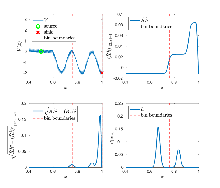
Figure 1: Using Algorithm 27 to compute the weighted ensemble bins ${\mathcal{B}}$ when the number of bins is $M=4$. We use $10^{6}$ iterations of Algorithm 27 with $\alpha=10^{5}$. Top left: Potential energy $V$ and bin boundaries when $M=4$. Top right: The vector ${\tilde{K}}{\tilde{h}}$ defining the objective function in Algorithm 27, where $\tilde{h}$ is the approximate Poisson solution. Note that ${\tilde{K}}{\tilde{h}}$ is nearly constant on each superbasin. Bottom left: (square root of) the vector $\tilde{K}\tilde{h}^{2}-(\tilde{K}\tilde{h})^{2}$ involved in the mutation variance optimization in Algorithm 2. Bottom right: Approximate steady state distribution $\tilde{\mu}$. All plots have been cropped at $x>0.4$, where the values of $\tilde{K}\tilde{h}^{2}-(\tilde{K}\tilde{h})^{2}$ and $\tilde{\mu}$ are neglibigle and ${\tilde{K}}{\tilde{h}}$ is nearly constant.

We choose $120$ uniformly spaced microbins between $0$ and $1$,

$${\mathcal{M}}{\mathcal{B}}=\{[(p-1)/120,p/120]:i=1,\ldots,120\}.$$

(They are not actually disjoint, but they do not overlap so this is unimportant.)

The microbins correspond to the basins of attraction of $V$. A basin of attraction of $V$ is a set of initial conditions $x(0)$ for which $dx(t)/dt=-V^{\prime}(x(t))$ has a unique long-time limit. The microbins comprise $3$ larger metastable sets, defined in Section 3 above. These larger metastable sets, each comprised of many smaller basins of attraction, will be called superbasins. The microbins do not need to be basins of attraction: they only need to be sufficiently “small” to give useful estimates of $K$ and $h$. We choose microbins in this way to illustrate the qualitative features we expect from Markov state modeling, where the Markov states (or our microbins) are often basins of attraction. In this case, the bins might be clusters of Markov states corresponding to superbasins.

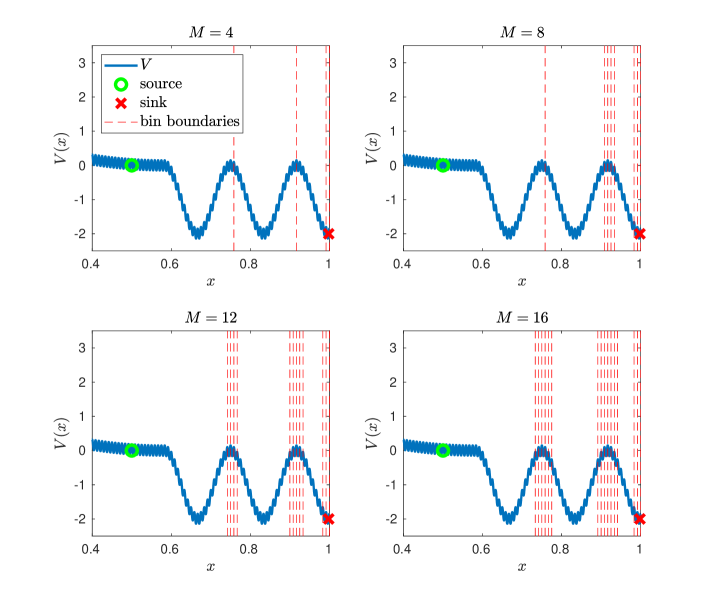
Figure 2: Increasing the value of $M$ in Algorithm 27. Plotted are weighted ensemble bins ${\mathcal{B}}$ computed using Algorithm 27 with $M=4,8,12,16$. For each value of $M$, we use $10^{6}$ iterations of Algorithm 27, with $\alpha$ tuned between $10^{5}$ and $10^{6}$. Note that with increasing $M$, additional bins are initially devoted to resolving the energy barrier between the two rightmost superbasins. Since the observable $f$ is the rightmost microbin, this is the most important energy barrier for the bins to resolve. Note that the multiple adjacent small bins for $M=16$ correspond to the steepest gradients of $\tilde{K}\tilde{h}$ in the top right of Figure 1. All plots have been cropped at $x>0.4$.

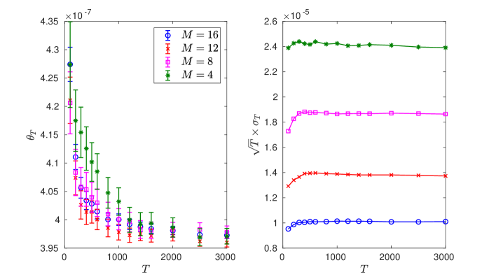
Figure 3: Varying the number $M$ of weighted ensemble bins in Algorithm 27. Left: Weighted ensemble running means $\theta_{T}$ vs. $T$ for Algorithm 1 with the optimal allocation and binning of Algorithms 2 and 27, when $M=4,8,12,16$. Values shown are averages over $10^{5}$ independent trials. Error bars are $\sigma_{T}/\sqrt{10^{5}}$, where $\sigma_{T}$ are the empirical standard deviations. Right: Scaled empirical standard deviations $\sqrt{T}\times\sigma_{T}$ vs. $T$ in the same setup. We use $N=40$ particles, and the bins correspond exactly to the ones in Figure 2. More bins is not always better, since with too many bins we return to the direct Monte Carlo regime; see Remark 5.1.

The kernel $K$ is defined as follows. First, let $K_{\delta t}$ be an Euler-Maruyama time discretization of (30) with time step $\delta t=2\times 10^{-5}$. We introduce a sink at the target state $[119/120,1]$ that recycles at a source $x=1/2$ via

$$\bar{K}_{\delta t}(x,dy)=\begin{cases}K_{\delta t}(\frac{1}{2},dy),&x\in[119/120,1]\\ K_{\delta t}(x,dy),&x\notin[119/120,1]\end{cases}.$$

Then we define $K$ as a $\Delta t$-skeleton of $\bar{K}_{\delta t}$ where $\Delta t=10$,

(31) $$K=\bar{K}_{\delta t}^{10}.$$

This just means we take $10$ Euler-Maruyama [37] time steps in the mutation step of Algorithm 1. The Hill relation [5] shows that, if $(\bar{X}_{n})_{n\geq 0}$ is a Markov chain with kernel either ${K}_{\delta t}$ or $\bar{K}_{\delta t}$ and $\bar{\tau}=\inf\{n\geq 0:\bar{X}_{n}\in[119/120,1]\}$, then

$${\mathbb{E}}[\bar{\tau}|\bar{X}_{0}=1/2]=\frac{1}{\mu([119/120,1])},$$

where $\mu$ is the stationary distribution of $K$. Thus if $\tau=\inf\{t>0:X_{t}\in[119/120,1]\}$,

$${\mathbb{E}}[\tau|X_{0}=1/2]\approx\frac{\delta t}{\mu([119/120,1])}.$$

By construction $\mu([119/120,1])$ is small (on the order $10^{-7}$), so it must be estimated with substantial precision to resolve the mean first passage time.

We will estimate the mean first passage time from $x=1/2$ to $x\in[119/120,1]$, the latter being the target state and rightmost microbin. Thus, we define $f$ as the characteristic function of this microbin, $f=\mathbbm{1}_{[119/200,1]}$, so that

$$\theta_{T}\approx\int f\,d\mu=\mu([119/120,1]).$$

Weighted ensemble then estimates the mean first passage time via

(32) $$\textup{Mean first passage time }={\mathbb{E}}[\tau|X_{0}=1/2]\approx\frac{\delta t}{\theta_{T}}.$$

We illustrate Algorithm 1 combined with Algorithms 2-27 in Figures 1-4. For Algorithms 2 and 27, to construct $\tilde{K}$, $\tilde{\mu}$, $\tilde{f}$ and $\tilde{h}$ as in Section 5, we compute the matrix $\tilde{K}$ using $10^{4}$ trajectories starting from each microbin’s midpoint, and we define $\tilde{f}_{120}=1$, $\tilde{f}_{p}=0$ for $1\leq p\leq 119$. The $p$th rows of $\tilde{K}$, $\tilde{\mu}$, $\tilde{f}$ and $\tilde{h}$ correspond to the microbin $[(p-1)/120,p/120]$. In Algorithm 27, to simplify visualization we enforce a condition that the bins must be connected regions. We initialize all our simulations with Algorithm 4 where $N_{\textup{init}}=120$, $\xi_{0}^{i}=(i-1/2)/120$, and $\omega^{i}=1/120$.

In Figure 1, we show the bins resulting from Algorithm 27, and plot the terms $\tilde{K}\tilde{h}$ and $\tilde{K}\tilde{h}^{2}-(\tilde{K}\tilde{h})^{2}$ appearing in the optimizations in Algorithms 2 and 27, along with the approximate steady state $\tilde{\mu}$. Note that the bins resolve the superbasins of $V$. In Figure 2, we explore what happens when the number $M$ of bins increases in Algorithm 27, finding that the bins begin to resolve the regions between superbasins, favoring regions closer to the support of $f$. As $M$ increases, the optimal allocation leads to particles having more children when they are near the dividing surfaces between the superbasins; to see why, compare the particle allocation in Algorithm 2 with the bottom left of Figure 1.

In Figure 3, we illustrate weighted ensemble with the optimized allocation and binning of Algorithms 2 and 27 when the number of bins increases from $M=4$ to $M=16$. Observe that $M=4$ bins is not enough to resolve the regions between the superbasins, but we still get a substantial gain over direct Monte Carlo (compare with Figure 4). With $M=16$ bins we resolve the regions between superbasins, further reducing the variance. The bins we use are exactly the ones in Figure 2.

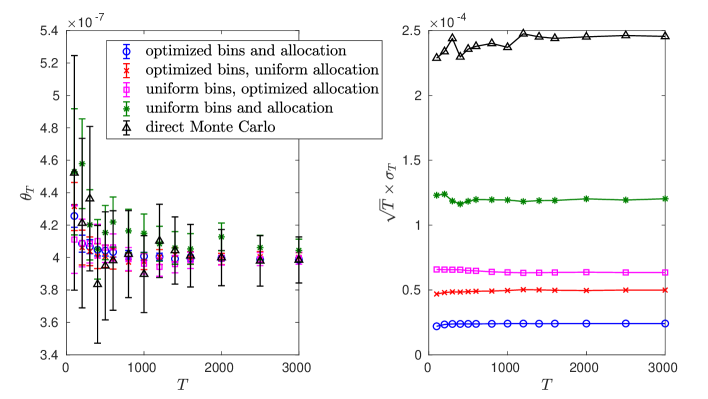
Figure 4: Comparison of direct Monte Carlo with weighted ensemble, where the bins and/or allocation are optimized, $M=4$, and $N=40$. Left: Weighted ensemble running means $\theta_{T}$ vs. $T$ for Algorithm 1 with the indicated choices for allocation and binning. Values shown are averages over $10^{5}$ independent trials. Error bars are $\sigma_{T}/\sqrt{10^{5}}$, where $\sigma_{T}$ are the empirical standard deviations. Right: Scaled empirical standard deviations $\sqrt{T}\times\sigma_{T}$ vs. $T$ in the same setup. By optimized bins, we mean the weighted ensemble bins ${\mathcal{B}}$ are chosen using Algorithm 27 with $M=4$. These optimized bins are exactly the ones plotted in top left of Figure 2. Optimized allocation means the particle allocation follows Algorithm 2. Uniform bins means that the bins are uniformly spaced on $[0,1]$, while uniform allocation means the particles are distributed uniformly among the occupied bins.

In Figure 4, we compare weighted ensemble with direct Monte Carlo when $M=4$. Direct Monte Carlo can be seen as a version of Algorithm 1 where each parent always has exactly one child, $C_{t}^{i}=1$ for all $t,i$. For weighted ensemble, we consider optimizing either or both of the bins and the allocation. When we do not optimize the bins, we consider uniform bins ${\mathcal{B}}=\{[0,40/120],[40/120,80/120],[80/120,1]\}.$ When we do not optimize the allocation, we consider uniform allocation, where we distribute particles evenly among the occupied bins, $N_{t}(u)\approx N/\#\{u\in{\mathcal{B}}:\omega_{t}(u)>0\}$. Notice the order of magnitude reduction in standard deviation compared with direct Monte Carlo for this relatively small number of bins.

In Figure 5, to illustrate the Hill relation, we plot the weighted ensemble estimates of the mean first passage time from our data in Figures 3 and 4 against the (numerically) exact value. The weighted ensemble estimates at small $T$ tend to exhibit a “bias” because the weighted ensemble has not yet reached steady state. As $T$ grows, this bias vanishes and the weighted ensemble estimates converge to the true mean first passage time. In the simple example in this section, we can directly compute the mean first passage time. For complicated biological problems, however, the first passage time can be so large that it is difficult to directly sample even once. In spite of this, the Hill relation reformulation can lead to useful estimates on much shorter time scales than the mean first passage time [1, 16, 64]. Indeed this is the case in Figure 5, where we get accurate estimates in a time horizon orders of magnitude smaller than the mean first passage time. This speedup can be attributed in part to the initialization in Algorithm 1. In general, there can also be substantial speedup from the Hill relation itself, independently of the initial condition [64].

Optimizing the bins and allocation together has the best performance. We expect that, as in this numerical example, when the number $M$ of bins is relatively small, optimizing the bins can be more important than optimizing the allocation. Optimizing only the allocation may lead to a less dramatic gain when the bins poorly resolve the landscape defined by $h$. On the other hand, for a large enough number $M$ of bins it may be sufficient just to optimize the allocation. We emphasize that more bins is not always better, since for a fixed number $N$ of particles, with too many bins we end up recovering direct Monte Carlo. See Remark 5.1 above.

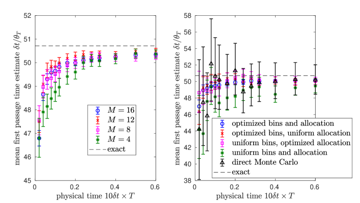
Figure 5: Illustration of the Hill relation for estimating the mean first passage time via (32). Left: the same data as in Figure 3, but $\theta_{T}$ is inverted and multiplied by $\delta t$ to estimate the mean first passage time, and error bars are adjusted accordingly. Right: the same data as in Figure 4, but $\theta_{T}$ is inverted and multiplied by $\delta t$ to estimate the mean first passage time, and error bars are adjusted accordingly. So that the $x$ and $y$ axes have the same units, we consider the “physical time” on the $x$-axis, defined as the total number, $T$, of selection steps of Algorithm 1 multiplied by the time, $10\delta t$, between selection steps (see (31)). In both plots, the “exact” value of the mean first passage time is obtained from $10^{5}$ independent samples of the first passage time $\bar{\tau}$. As in Figures 3 and 4, optimizing the bins and allocation has the best performance, and $M=16$ bins is better than $M=4,8,12$ bins, though more bins is not always better; see Remark 5.1.

7 Remarks and future work

This work presents new procedures for choosing the bins and particle allocation for weighted ensemble, building in part from ideas in [5]. The bins and particle allocation, together with the resampling times, completely characterize the method. Though we do not try to optimize the latter, we argue that there is no significant variance cost associated with taking small resampling times. Optimizing weighted ensemble is worthwhile when the optimized parameter choices lead to significantly more particles in important regions of state space, compared to a naive method. The corresponding gain, represented by the rule of thumb (28), can be expected to grow as the dimension increases. This is because in high dimension the pathways between metastable sets are narrow compared to the vast state space (see [59, 60] and the references in the Introduction).

Though our interest is in steady state calculations, many of our ideas could just as well be applied to a finite time setup. Our practical interest in steady state arises from the computation of mean first passage times via the Hill relation. On the mathematical side, general importance sampling particle methods with the unbiased property of Theorem 3.1 are often not appropriate for steady state sampling. (By general methods, we mean methods for nonreversible Markov chains, or Markov chains with a steady state that is not known up to a normalization factor [40].) Indeed as we explain in our companion article [4], standard sequential Monte Carlo methods can suffer from variance explosion at large times, even for carefully designed resampling steps. So this article could be an important advance in that direction.

We conclude by discussing some open problems. The implementation of the algorithms in this article to complex, high dimensional problems will require substantial effort and modification to the software in [66]. The aim of this article is to lay the groundwork for such applications. On a more theoretical note, there remain some questions regarding parameter optimization. We could consider adaptive/non-spatial bins instead of fixed bins as in Algorithm 27, for instance bins chosen via $k$-means on the values of $Kh$ of the $N$ particles. Also, we choose a number $M$ of weighted ensemble bins and number $N$ of particles a priori. It remains open how to pick the best value of $M$ for a given number, $N$, of particles, and fixed computational resources. Using only the variance analysis above, a straightforward answer to this question can probably only be obtained in the large $N$ asymptotic regime. More analysis is then needed, since we generally have small $N$. We could also optimize over both $N$ and $M$, or over $N$, $M$ and a total number $S$ of independent simulations, subject to a fixed computational budget. We leave these questions to future work.

8 Appendix

In this appendix, we describe residual resampling, and we draw a connection between mutation variance minimization and sensitivity.

8.1 Residual resampling

Recall that in Algorithm 1 we assumed residual resampling is used to get the number of children $(C_{t}^{j})^{j=1,\ldots,N}$ of each particle $\xi_{t}^{j}$ at each time $t$. We could also use residual resampling to compute $R_{t}(u)^{u\in{\mathcal{B}}}$ in Algorithm 2. For the reader’s convenience, we describe residual resampling in Algorithm 5. Recall $\lfloor x\rfloor$ is the floor function (the greatest integer $\leq x$).

Algorithm 5 Residual resampling

To generate $n$ samples $\{N_{i}:i\in{\mathcal{I}}\}$ from a distribution $\{d_{i}:i\in{\mathcal{I}}\}$ with $\sum_{i\in{\mathcal{I}}}d_{i}=1$:

• Define $\delta_{i}=nd_{i}-\lfloor nd_{i}\rfloor$ and let $\delta=\sum_{i\in{\mathcal{I}}}\delta_{i}$.

• Sample $\{R_{i}:i\in{\mathcal{I}}\}$ from the multinomial distribution with $\delta$ trials and event probabilities $\delta_{i}/\delta$, $i\in{\mathcal{I}}$. In detail,

  $${\mathbb{P}}(R_{i}=r_{i},\,i\in{\mathcal{I}})=\mathbbm{1}_{\sum_{i\in{\mathcal{I}}}r_{i}=\delta}\frac{\delta!}{\prod_{i\in{\mathcal{I}}}r_{i}!}\prod_{i\in{\mathcal{I}}}(\delta_{i}/\delta)^{r_{i}}.$$

• Define $N_{i}=\lfloor nd_{i}\rfloor+R_{i}$, $i\in{\mathcal{I}}$.

8.2 Intuition behind mutation variance minimization

The goal of this section is to give some intuition for the strategy (20), which chooses the particle allocation to minimize mutation variance, by introducing a connection with sensitivity of the stationary distribution $\mu$ to perturbations of $K$. In this section we make the simplifying assumption that state space is finite, and each point of state space is a microbin. Thus $K=(K_{pq})_{p,q\in{\mathcal{M}}{\mathcal{B}}}$ is a finite stochastic matrix. The Poisson solution $h$ defined in (15) satisfies $(I-K)h=f-(f^{T}\mu)\mathbbm{1}$ and $h^{T}\mu=0$, or equivalently

(33) $$h=\sum_{s=0}^{\infty}K^{s}\bar{f},\qquad\bar{f}=f-(f^{T}\mu)\mathbbm{1}.$$

where $h=(h_{p})_{p\in{\mathcal{M}}{\mathcal{B}}}$, $f=(f_{p})_{p\in{\mathcal{M}}{\mathcal{B}}}$, $\bar{f}=(\bar{f}_{p})_{p\in{\mathcal{M}}{\mathcal{B}}}$, and $\mu=(\mu_{p})_{p\in{\mathcal{M}}{\mathcal{B}}}$ are column vectors, and $\mathbbm{1}=\sum_{p\in{\mathcal{M}}{\mathcal{B}}}e_{p}$ is the all ones column vector. Here, $I$ is the identity matrix, and $(e_{p})_{p\in{\mathcal{M}}{\mathcal{B}}}$ is the column vector with $1$ in the $p$th entry and $0$’s elsewhere.

We write $\mu(Q)$ for the stationary distribution of an irreducible stochastic matrix $Q=(Q_{pq})_{p,q\in{\mathcal{M}}{\mathcal{B}}}$. More precisely, $\mu(Q)$ denotes a continuously differentiable extension of $Q\mapsto\mu(Q)$ to an open neighborhood of the space of $\#{\mathcal{M}}{\mathcal{B}}\times\#{\mathcal{M}}{\mathcal{B}}$ irreducible stochastic matrices which satisfies $\mu(Q)^{T}Q=\mu(Q)^{T}$ and $\mu(Q)^{T}\mathbbm{1}=1$ whenever $Q\mathbbm{1}=\mathbbm{1}$. See [52] for details and a proof of existence of this extension. Abusing notation, we still write $\mu$ with no matrix argument to denote the stationary distribution $\mu(K)$ of $K$.

Theorem 8.1.

Let $\lambda(u)>0$ be such that $\sum_{u\in{\mathcal{B}}}\lambda(u)=1$. For each $u\in{\mathcal{B}}$, let $\nu(u)=(\nu(u)_{p})_{p\in{\mathcal{M}}{\mathcal{B}}}$ be a vector satisfying $\nu(u)_{p}\geq 0$ for $p\in{\mathcal{M}}{\mathcal{B}}$, $\nu(u)_{p}=0$ for $p\notin u$, and $\sum_{p\in u}\nu(u)_{p}=1$. Let $A(u)$ be a random matrix with the distribution

(34) $${\mathbb{P}}\left(A(u)=e_{p}e_{q}^{T}-e_{p}e_{p}^{T}K\right)=\nu(u)_{p}K_{pq},\qquad\text{if }p\in u,\,q\in{\mathcal{M}}{\mathcal{B}}.$$

Let $A(u)^{(n)}$ be independent copies of $A$, for $u\in{\mathcal{B}}$ and $n=1,2,\ldots$. Define

(35) $$B^{(N)}=\sqrt{N}\sum_{u\in{\mathcal{B}}}\frac{1}{\lfloor N\lambda(u)\rfloor}\sum_{n=1}^{\lfloor N\lambda(u)\rfloor}A(u)^{(n)}.$$

Then

(36) $$\begin{split}&\lim_{N\to\infty}{\mathbb{E}}\left[\left(\left.\frac{d}{d\epsilon}\mu(K+\epsilon B^{(N)})^{T}\right|_{\epsilon=0}f\right)^{2}\right]\\ &\qquad=\sum_{u\in{\mathcal{B}}}\lambda(u)^{-1}\sum_{p\in u}\nu(u)_{p}\mu_{p}^{2}\left[(Kh^{2})_{p}-(Kh)_{p}^{2}\right].\end{split}$$

We now interpret Theorem 8.1 from the point of view of particle allocation. Note that $A(u)$ is a centered sample of of $K$ obtained by picking a microbin $p\in u$ according to the distribution $\nu(u)$, and then simulating a transition from $p$ via $K$. By a centered sample, we mean that we adjust $A(u)$ by subtracting by its mean, so that $A(u)$ has mean zero. The mean of $[(d/d\epsilon)\mu(K+\epsilon A(u))^{T}|_{\epsilon=0}f]^{2}$ measures the sensitivity of $\int f\,d\mu=f^{T}\mu$ to sampling from bin $u$ according to the distribution $\nu(u)$. Similarly, the mean of $[(d/d\epsilon)\mu(K+\epsilon B^{(N)})^{T}|_{\epsilon=0}f]^{2}$ measures the sensitivity of $\int f\,d\mu$ corresponding to sampling from each bin $u\in{\mathcal{B}}$ exactly $\lfloor N\lambda(u)\rfloor$ times according to the distributions $\nu(u)$. Appropriately normalizing the latter in the limit $N\to\infty$ leads to (LABEL:sensitivity). The sensitivity in (LABEL:sensitivity) is minimized over $\lambda(u)^{u\in{\mathcal{B}}}$ when

(37) $$N\lambda(u)=\dfrac{N\sqrt{\sum_{p\in u}\nu(u)_{p}\mu_{p}^{2}\left[(Kh^{2})_{p}-(Kh)_{p}^{2}\right]}}{\sum_{u\in{\mathcal{B}}}\sqrt{\sum_{p\in u}\nu(u)_{p}\mu_{p}^{2}\left[(Kh^{2})_{p}-(Kh)_{p}^{2}\right]}}.$$

In light of the discussion above, we think of $N\lambda(u)^{u\in{\mathcal{B}}}$ in (37) as a particle allocation. Note that this resembles our formula (20) for the optimal weighted ensemble particle allocation. We now try to make a connection between (20) and (37).

We first consider a simple case. Suppose the bins are equal to the microbins, ${\mathcal{M}}{\mathcal{B}}={\mathcal{B}}$. Since we assume here that every point in state space is a microbin, this means that every point of state space is also a bin. In particular the distributions $\nu(u)$ are trivial: $\nu(u)_{p}=1$ whenever $p\in{\mathcal{M}}{\mathcal{B}}$ with $p=u$. To make (37) agree with (20), we need $\mu_{p}=\omega_{t}(u)$ when $p=u$. Of course this equality does not hold. It is true that $\mu_{p}\approx\omega_{t}(u)$ when $p=u$ is a reasonable approximation, but only in the asymptotic where $N,t\to\infty$. To see why this is so, note that the unbiased property and ergodicity show that $\lim_{t\to\infty}{\mathbb{E}}[\omega_{t}(u)]=\mu_{p}$ when $p=u$; provided an appropriate law of large numbers also holds, $\lim_{t\to\infty}\lim_{N\to\infty}\omega_{t}(u)=\mu_{p}$. Recall, though, that we are interested in relatively small $N$, due to the high cost of particle evolution.

For the general case, where ${\mathcal{M}}{\mathcal{B}}\neq{\mathcal{B}}$ and bins contain multiple points in state space, we see no direct connection between the allocation formulas (37) and (20). Indeed, to make an analogy between this sensitivity calculation and weighted ensemble, we should have $\nu(u)_{p}=\sum_{i:\xi_{t}^{i}\in p}\omega_{t}^{i}/\omega_{t}(u)$. Or in other words, we should consider perturbations that correspond to sampling from the bins according to particle weights, in accordance with Algorithm 1. But putting $\nu(u)_{p}=\sum_{i:\xi_{t}^{i}\in p}\omega_{t}^{i}/\omega_{t}(u)$ in (37) gives something quite different from (20). So while the sensitivity minimization formula (37) is qualitatively similar to our mutation variance minimization formula (20), the two are not actually the same.

8.3 Proof of Theorem 8.1

We begin by noting the following.

(38) $$\text{If }v^{T}\mathbbm{1}=0,\quad\text{then}\quad g^{T}(I-K)=v^{T},\,\,g^{T}\mathbbm{1}=0\quad\Longleftrightarrow\quad g^{T}=\sum_{s=0}^{\infty}v^{T}K^{s}.$$

Like (33), this follows from ergodicity of $K$. See for instance [31].

Lemma 8.2.

Suppose $A$ is a matrix with $A\mathbbm{1}=0$. Then

$$\left.\frac{d}{d\epsilon}\mu(K+\epsilon A)\right|_{\epsilon=0}f=\mu^{T}Ah.$$

Proof 8.3.

Since $\mu(K+\epsilon A)^{T}(K+\epsilon A)=\mu(K+\epsilon A)^{T}$, we have

$$0=\left.\frac{d}{d\epsilon}\mu(K+\epsilon A)^{T}(I-K-\epsilon A)\right|_{\epsilon=0}=\left.\frac{d}{d\epsilon}\mu(K+\epsilon A)^{T}\right|_{\epsilon=0}(I-K)-\mu^{T}A.$$

Thus

(39) $$\left.\frac{d}{d\epsilon}\mu(K+\epsilon A)^{T}\right|_{\epsilon=0}(I-K)=\mu^{T}A.$$

Moreover since $\mu(Q)^{T}\mathbbm{1}=1$ for any stochastic matrix $Q$,

(40) $$0=\left.\frac{d}{d\epsilon}\mu(K+\epsilon A)^{T}\mathbbm{1}\right|_{\epsilon=0}\\ =\left.\frac{d}{d\epsilon}\mu(K+\epsilon A)^{T}\right|_{\epsilon=0}\mathbbm{1}.$$

Now by (33), (38), (39), and (40),

$$\left.\frac{d}{d\epsilon}\mu(K+\epsilon A)^{T}\right|_{\epsilon=0}f =\sum_{s=0}^{\infty}\mu^{T}AK^{s}f$$

$$=\mu^{T}A\sum_{s=0}^{\infty}K^{s}\bar{f}=\mu^{T}Ah,$$

where the last line above uses $AK^{s}\mathbbm{1}=A\mathbbm{1}=0$ to replace $f$ with $\bar{f}=f-\mu^{T}f\mathbbm{1}$.

Lemma 8.4.

Suppose $(A^{(n)})^{n=1,\ldots,N}$ are matrices such that (i) $(A^{(n)})^{n=1,\ldots,N}$ are independent over $n$, (ii) $A^{(n)}\mathbbm{1}=0$ for all $n$, and (iii) ${\mathbb{E}}[A^{(n)}]=0$ for all $n$. Then

$${\mathbb{E}}\left[\left(\frac{d}{d\epsilon}\left.\mu\left(K+\epsilon\sum_{n=1}^{N}A^{(n)}\right)^{T}\right|_{\epsilon=0}f\right)^{2}\right]=\sum_{n=1}^{N}{\mathbb{E}}\left[\left(\frac{d}{d\epsilon}\left.\mu\left(K+\epsilon A^{(n)}\right)^{T}\right|_{\epsilon=0}f\right)^{2}\right].$$

Proof 8.5.

Since $\mu$ is continuously differentiable,

(41) $$\frac{d}{d\epsilon}\left.\mu\left(K+\epsilon\sum_{n=1}^{N}A^{(n)}\right)^{T}\right|_{\epsilon=0}f=\sum_{n=1}^{N}\frac{d}{d\epsilon}\left.\mu\left(K+\epsilon A^{(n)}\right)^{T}\right|_{\epsilon=0}f.$$

By (ii)-(iii) and Lemma 8.2, ${\mathbb{E}}\left[\frac{d}{d\epsilon}\left.\mu\left(K+\epsilon A^{(n)}\right)^{T}\right|_{\epsilon=0}f\right]=0$ for all $n$. So by (i),

(42) $${\mathbb{E}}\left[\frac{d}{d\epsilon}\left.\mu\left(K+\epsilon A^{(n)}\right)^{T}\right|_{\epsilon=0}f\frac{d}{d\epsilon}\left.\mu\left(K+\epsilon A^{(m)}\right)^{T}\right|_{\epsilon=0}f\right]=0,\qquad\text{if }n\neq m.$$

The result follows by combining (41) and (42).

Lemma 8.6.

Let $A(u)$ be a random matrix with the distribution (34). Then

$${\mathbb{E}}\left[\left(\left.\frac{d}{d\epsilon}{\mu}(K+\epsilon A(u))^{T}\right|_{\epsilon=0}f\right)^{2}\right]=\sum_{p\in u}\nu(u)_{p}\mu_{p}^{2}\left[(Kh^{2})_{p}-(Kh)_{p}^{2}\right].$$

Proof 8.7.

Note that $A(u)\mathbbm{1}=(e_{p}e_{q}^{T}-e_{p}e_{p}^{T}K)\mathbbm{1}=0$ since $K\mathbbm{1}=\mathbbm{1}$. So by Lemma 8.2,

$$\left.\frac{d}{d\epsilon}\mu\left(K+\epsilon A(u)\right)\right|_{\epsilon=0}^{T}f=\mu^{T}A(u)h.$$

From this and (34),

$${\mathbb{E}}\left[\left(\frac{d}{d\epsilon}\left.{\mu}(K+\epsilon A(u))^{T}\right|_{\epsilon=0}f\right)^{2}\right] =\sum_{p\in u}\sum_{q\in{\mathcal{M}}{\mathcal{B}}}\nu(u)_{p}K_{pq}\left[\mu^{T}(e_{p}e_{q}^{T}-e_{p}e_{p}^{T}K)h\right]^{2}$$

$$=\sum_{p\in u}\nu(u)_{p}\mu_{p}^{2}\sum_{q\in{\mathcal{M}}{\mathcal{B}}}K_{pq}\left[(e_{q}^{T}-e_{p}^{T}K)h\right]^{2}$$

$$=\sum_{p\in u}\nu(u)_{p}\mu_{p}^{2}\sum_{q\in{\mathcal{M}}{\mathcal{B}}}K_{pq}\left[(Kh)_{p}^{2}+h_{q}^{2}-2(Kh)_{p}h_{q}\right]$$

$$=\sum_{p\in u}\nu(u)_{p}\mu_{p}^{2}\left[(Kh^{2})_{p}-(Kh)_{p}^{2}\right].$$

We are now ready to prove Theorem 8.1.

Proof 8.8 (Proof of Theorem 8.1).

By Lemmas 8.4 and 8.6,

(43) $$\begin{split}&{\mathbb{E}}\left[\left(\frac{d}{d\epsilon}\left.\mu\left(K+\epsilon B^{(N)}\right)^{T}\right|_{\epsilon=0}f\right)^{2}\right]\\ &=N\sum_{u\in{\mathcal{B}}}\frac{1}{\lfloor N\lambda(u)\rfloor^{2}}\sum_{n=1}^{\lfloor N\lambda(u)\rfloor}{\mathbb{E}}\left[\left(\frac{d}{d\epsilon}\left.\mu\left(K+\epsilon A(u)^{(n)}\right)^{T}\right|_{\epsilon=0}f\right)^{2}\right]\\ &=\sum_{u\in{\mathcal{B}}}\frac{N}{\lfloor N\lambda(u)\rfloor}\sum_{p\in u}\nu(u)_{p}\mu_{p}^{2}\left[(Kh^{2})_{p}-(Kh)_{p}^{2}\right].\end{split}$$

The result follows by letting $N\to\infty$.

References

- [1] U. Adhikari, B. Mostofian, J. Copperman, S.R. Subramanian, A.A. Petersen, and D.M. Zuckerman. Computational Estimation of Microsecond to Second Atomistic Folding Times. J. Am. Chem. Soc. 141(16), 6519–6526, 2019.
- [2] R. J. Allen, D. Frenkel, and P. R. ten Wolde. Forward flux sampling-type schemes for simulating rare events: Efficiency analysis. The Journal of chemical physics, 124(19):194111, 2006.
- [3] D.F. Anderson and T.G. Kurtz. Continuous Time Markov Chain Models for Chemical Reaction Networks, Design and Analysis of Biomolecular Circuits, pgs. 3–42, 2011.
- [4] D. Aristoff. An ergodic theorem for weighted ensemble. arXiv preprint arXiv:1906.00856.
- [5] D. Aristoff. Analysis and optimization of weighted ensemble sampling. ESAIM: Mathematical Modelling and Numerical Analysis 52(2018): 1219–1238, 2018.
- [6] M. Balesdent J. Marzat J. Morio, D. Jacquemart. Optimisation of interacting particle systems for rare event estimation. Computational Statistics & Data Analysis 66:117–128, 2013.
- [7] J. M. Bello-Rivas and R. Elber. Exact milestoning. The Journal of Chemical Physics, 142(9):03B602_1, 2015.
- [8] D. Bhatt, B. W. Zhang, and D. M. Zuckerman. Steady-state simulations using weighted ensemble path sampling. The Journal of chemical physics, 133(1):014110, 2010.
- [9] C.-E. Bréhier, T. Lelièvre, and M. Rousset. Analysis of Adaptive Multilevel Splitting algorithms in an idealized case. ESAIM P&S, 19, 361–394, 2015.
- [10] C.-E. Bréhier, M. Gazeau, L. Goudenège, T. Lelièvre, and M. Rousset. Unbiasedness of some generalized Adaptive Multilevel Splitting algorithms. Annals of Applied Probability, 26(6): 3559–3601, 2016.
- [11] F. Cérou, A. Guyader, T. Lelièvre, and D. Pommier. A multiple replica approach to simulate reactive trajectories. J. Chem. Phys. 134: 054108, 2011.
- [12] L. T. Chong, A. S. Saglam, and D. M. Zuckerman. Path-sampling strategies for simulating rare events in biomolecular systems. Current opinion in structural biology, 43:88–94, 2017.
- [13] H. Chraibi, A. Dutfoy, T. Galtier, and J. Garnier. Optimal input potential functions in the interacting particle system method. arXiv preprint arXiv:1811.10450, 2018.
- [14] P. Collet, S. Martínez, and J. San Martín. Quasi-Stationary Distributions: Markov Chains, Diffusions and Dynamical Systems. Springer Science & Business Media, 2012.
- [15] J. Copperman and D.M. Zuckerman. Accelerated estimation of long-timescale kinetics by combining weighted ensemble simulation with Markov model “microstates” using non-Markovian theory. arXiv preprint arXiv:1903.04673.
- [16] J. Copperman, D. Aristoff, D.E. Makarov, G. Simpson, and D.M. Zuckerman. Transient probability currents provide upper and lower bounds on non-equilibrium steady-state currents in the Smoluchowski picture arXiv preprint arXiv:1810.09964.
- [17] R. Costaouec, H. Feng, J. Izaguirre, and E. Darve. Analysis of the accelerated weighted ensemble methodology. Discrete and Continuous Dynamical Systems, pages 171–181, 2013.
- [18] E. Darve and E. Ryu. Computing reaction rates in bio-molecular systems using discrete macro-states. arXiv preprint arXiv:1307.0763, 2013.
- [19] P. Del Moral. Feynman-kac formulae: genealogical and interacting particle approximations. Probability and Its Applications, Springer, 2004.
- [20] P. Del Moral and A. Doucet. Particle methods: An introduction with applications. In ESAIM: proceedings, volume 44, pages 1–46. EDP Sciences, 2014.
- [21] P. Del Moral, J. Garnier, et al. Genealogical particle analysis of rare events. The Annals of Applied Probability, 15(4):2496–2534, 2005.
- [22] A. R. Dinner, J. C. Mattingly, J. O. Tempkin, B. Van Koten, and J. Weare. Trajectory stratification of stochastic dynamics. arXiv preprint arXiv:1610.09426, 2016.
- [23] R. M. Donovan, A. J. Sedgewick, J. R. Faeder, and D. M. Zuckerman. Efficient stochastic simulation of chemical kinetics networks using a weighted ensemble of trajectories. The Journal of chemical physics, 139(11):09B642_1, 2013.
- [24] J.L. Doob. Stochastic processes. Wiley, 1953.
- [25] J.L. Doob. Regularity properties of certain families of chance variables. Transactions of the American Mathematical Society. 47 (3): 455–486, 1940.
- [26] R. Douc and O. Cappé. Comparison of resampling schemes for particle filtering. In Image and Signal Processing and Analysis, 2005. ISPA 2005. Proceedings of the 4th International Symposium on, pages 64–69. IEEE, 2005.
- [27] R. Douc, E. Moulines, and D. Stoffer. Nonlinear Time Series Theory, Methods, and Applications with R Examples. CRC press, 2015.
- [28] A. Doucet, N. De Freitas, and N. Gordon. Sequential monte carlo methods in practice. Series statistics for engineering and information science, Springer, 2001.
- [29] R. Durrett. Probability: theory and examples. Cambridge university press, 2019.
- [30] D. R. Glowacki, E. Paci, and D. V. Shalashilin. Boxed molecular dynamics: decorrelation time scales and the kinetic master equation. Journal of chemical theory and computation, 7(5):1244–1252, 2011.
- [31] G.H. Golub and C.D. Meyer, Using the QR Factorization and Group Inversion to Compute, Differentiate, and Estimate the Sensitivity of Stationary Probabilities for Markov Chains. SIAM. J. on Algebraic and Discrete Methods 7(2), 273–281, 1986.
- [32] T. L. Hill. Free energy transduction and biochemical cycle kinetics. Courier Corporation, 2005.
- [33] H. Hofmann and F.A. Ivanyuk. Mean first passage time for nuclear fission and the emission of light particles. Physical review letters 90(13): 132701, 2003.
- [34] G. A. Huber and S. Kim. Weighted-ensemble brownian dynamics simulations for protein association reactions. Biophysical journal, 70(1):97–110, 1996.
- [35] B.E. Husic and V.S. Pande. Markov State Models: From an Art to a Science. J. Am. Chem. Soc. 140(7), 2386–2396, 2018.
- [36] D. Jacquemart and J. Morio. Tuning of adaptive interacting particle system for rare event probability estimation. Simulation Modelling Practice and Theory 66:36–49, 2016.
- [37] P.E. Kloeden and E. Platen. Numerical Solution of Stochastic Differential Equations. Springer, 1992.
- [38] H. Kushner and G. G. Yin. Stochastic approximation and recursive algorithms and applications, volume 35. Springer Science & Business Media, 2003.
- [39] T. Lelièvre. Two mathematical tools to analyze metastable stochastic processes. Numerical Mathematics and Advanced Applications 791–810, 2011.
- [40] T. Lelièvre and G. Stoltz. Partial differential equations and stochastic methods in molecular dynamics. Acta Numerica 25:681–880, 2016.
- [41] Lloyd, Stuart P. Least squares quantization in PCM. IEEE Transactions on Information Theory (28): 129-137, 1982.
- [42] R. Metzler, G. Oshanin, and S. Redner, eds. First-passage phenomena and their applications. World Scientific, 2014.
- [43] S.P. Meyn and R.L. Tweedie. Stability of Markovian processes II: continuous-time processes and sampled chains. Adv. Appl. Prob. 25, 487–517, 1993.
- [44] E. Nummelin. On the Poisson equation in the potential theory of a single kernel. Math. Scand. 68, 59–82, 1991.
- [45] V.S. Pande, K. Beauchamp, and G.R. Bowman. Everything you wanted to know about Markov State Models but were afraid to ask. Methods. 52(1): 99–105, 2010.
- [46] A. Rojnuckarin, S. Kim, and S. Subramaniam. Brownian dynamics simulations of protein folding: access to milliseconds time scale and beyond. Proceedings of the National Academy of Sciences, 95(8):4288–4292, 1998.
- [47] A. Rojnuckarin, D. R. Livesay, and S. Subramaniam. Bimolecular reaction simulation using weighted ensemble brownian dynamics and the university of houston brownian dynamics program. Biophysical journal, 79(2):686–693, 2000.
- [48] M. Sarich, F. Noé and C. Schütte. On the approximation quality of Markov State Models. Multiscale Model. Simul. 8(4): 1154–1177, 2010.
- [49] C. Schütte and M. Sarich. Metastability and Markov State Models in Molecular Dynamics. Courant Lecture Notes, AMS, 2013.
- [50] G. Stoltz, M. Rousset, et al. Free energy computations: A mathematical perspective. World Scientific, 2010.
- [51] E. Suárez, S. Lettieri, M.C. Zwier, C.A. Stringer, S.R. Subramanian, L.T. Chong, and D.M. Zuckerman. Simultaneous Computation of Dynamical and Equilibrium Information Using a Weighted Ensemble of Trajectories. J. Chem. Theory. Comput. 10(7), 2658–2667, 2014.
- [52] E. Thiede, B. Van Koten, and J. Weare. Sharp entrywise perturbation bounds for Markov chains. SIAM J Matrix Anal Appl. 36(3): 917–941, 2015.
- [53] T. S. van Erp, D. Moroni, and P. G. Bolhuis. A novel path sampling method for the calculation of rate constants. The Journal of chemical physics, 118(17):7762–7774, 2003.
- [54] E. Vanden-Eijnden and M. Venturoli. Exact rate calculations by trajectory parallelization and tilting. The Journal of chemical physics, 131(4):044120, 2009.
- [55] E. Vanden-Eijnden, M. Venturoli, G. Ciccotti, and R. Elber. On the assumptions underlying milestoning. The Journal of chemical physics, 129(17):174102, 2008.
- [56] A. Warmflash, P. Bhimalapuram, and A. R. Dinner. Umbrella sampling for nonequilibrium processes. The Journal of chemical physics, 2007.
- [57] R.J. Webber, D.A. Plotkin, M.E. O’Neill, D.S. Abbot, and J. Weare. Practical rare event sampling for extreme mesoscale weather. arXiv preprint arXiv:1904.03464, 2019.
- [58] R.J. Webber. Unifying Sequential Monte Carlo with Resampling Matrices. arXiv preprint arXiv:1903.12583, 2019.
- [59] Weinan E, W. Ren and E. Vanden-Eijnden. Transition pathways in complex systems: Reaction coordinates, isocommittor surfaces, and transition tubes. Chemical Physics Letters 413:242–247, 2005.
- [60] Weinan E. and E. Vanden-Eijnden. Transition-path theory and path-finding algorithms for the study of rare events. Annual Review of Physical Chemistry 61:391–420, 2010.
- [61] J. Wouters and F. Bouchet. Rare event computation in deterministic chaotic systems using genealogical particle analysis. Journal of Physics A: Mathematical and Theoretical 49(37):374002, 2016.
- [62] B. W. Zhang, D. Jasnow, and D. M. Zuckerman. Efficient and verified simulation of a path ensemble for conformational change in a united-residue model of calmodulin. Proceedings of the National academy of Sciences, 104(46):18043–18048, 2007.
- [63] B. W. Zhang, D. Jasnow, and D. M. Zuckerman. The “weighted ensemble” path sampling method is statistically exact for a broad class of stochastic processes and binning procedures. The Journal of chemical physics, 132(5):054107, 2010.
- [64] D.M. Zuckerman, http://www.physicallensonthecell.org/discrete-state-kinetics-and-markov-models, equation (34).
- [65] D.M. Zuckerman and L.T. Chong. Weighted Ensemble Simulation: Review of Methodology, Applications, and Software. Annu. Rev. Biophys. 46: 43–57, 2017.
- [66] M.C. Zwier, J. L. Adelman, J. W. Kaus, A. J. Pratt, K. F. Wong, N. S. Rego, E. Suárez, S. Lettieri, D. W. Wang, M. Grabe, D. M. Zuckerman, and L. T. Chong. Westpa github pack. https://westpa.github.io/westpa/, 2015–.
- [67] M. C. Zwier, J. L. Adelman, J. W. Kaus, A. J. Pratt, K. F. Wong, N. B. Rego, E. Suárez, S. Lettieri, D. W. Wang, M. Grabe, D.M. Zuckerman, andL.T. Chong. Westpa: An interoperable, highly scalable software package for weighted ensemble simulation and analysis. Journal of chemical theory and computation, 11(2):800–809, 2015.