Gravitational radiation in Infinite Derivative Gravity
and connections to Effective Quantum Gravity

Abstract

The Hulse-Taylor binary provides possibly the best test of GR to date. We find the modified quadrupole formula for Infinite Derivative Gravity (IDG). We investigate the backreaction formula for propagation of gravitational waves, found previously for Effective Quantum Gravity (EQG) for a flat background and extend this calculation to a de Sitter background for both EQG and IDG. We put tighter constraints on EQG using new LIGO data. We also find the power emitted by a binary system within the IDG framework for both circular and elliptical orbits and use the example of the Hulse-Taylor binary to show that IDG is consistent with GR.

General Relativity (GR) has been spectacularly successful in experimental tests, notably in the recent detection of gravitational waves Abbott:2016blz . One of the most renowned tests is the Hulse-Taylor binary. The way the orbital period of these two stars changes over time depends on the gravitational radiation emitted. This matches the GR prediction to within 0.2% Weisberg:2016jye .

However, GR breaks down at short distances where it produces singularities. The first attempts to modify gravity by altering the action failed because they generated ghosts, which are excitations with negative kinetic energy stelle:1977 . Infinite Derivative Gravity (IDG) Tseytlin:1995uq ; Biswas:2005qr ; Biswas:2011ar ; Biswas:2016etb ; Siegel:2003vt ; Biswas:2005qr ; Biswas:2011ar ; Biswas:2016etb ; Buoninfante:2016iuf ; Talaganis:2014ida ; Modesto:2011kw ; Modesto:2012ys ; Biswas:2005qr ; Biswas:2011ar ; Edholm:2016hbt ; Conroy:2017nkc ; Edholm:2018dsf ; Conroy:2014eja ; Cornell:2017irh ; Biswas:2013cha ; Calcagni:2013vra ; Biswas:2010zk ; Biswas:2012bp ; Koshelev:2012qn ; Koshelev:2013lfm ; Biswas:2016etb ; Biswas:2016egy ; Conroy:2015wfa ; Edholm:2016seu ; Briscese:2012ys ; Teimouri:2016ulk ; Koshelev:2016xqb ; Craps:2014wga ; Talaganis:2014ida ; Talaganis:2017tnr ; Conroy:2014dja avoids this fate while also allowing us the possibility to not produce singularities.

IDG has the action Biswas:2011ar

$$\mathcal{L}=\frac{\sqrt{-g}}{2}\bigg{[} M^{2}_{P}R\ +RF_{1}(\Box)R+R_{\mu\nu}F_{2}(\Box)R^{\mu\nu}$$ (1)

$$+C_{\mu\nu\rho\lambda}F_{3}(\Box)C^{\mu\nu\rho\lambda}\bigg{]},$$

where $M_{P}$ is the Planck mass, $R$ is the Ricci scalar, $R_{\mu\nu}$ is the Ricci tensor and $C_{\mu\nu\rho\lambda}$ is the Weyl tensor. Each $F_{i}(\Box)$ is an infinite series of the d’Alembertian operator $\Box=g^{\mu\nu}\nabla_{\mu}\nabla_{\nu}$ i.e. $F_{i}(\Box)=\sum_{n=0}^{\infty}f_{i_{n}}\Box^{n}/M^{2n}$, where the $f_{i_{n}}$s are dimensionless coefficients and $M$ is the mass scale of the theory, which dictates the length scales below which the additional terms come into play.

The propagator $\Pi_{\text{IDG}}$ around a flat background in terms of the spin projection operators is modified as follows Biswas:2011ar

$$\Pi_{\text{IDG}}=\frac{P^{2}}{a(k^{2})}+\frac{P^{0}_{s}}{a(k^{2})-3c(k^{2})}\underset{a=c}{=}\frac{\Pi_{\text{GR}}}{a(k^{2})}$$ (2)

where $a$ and $c$ (given in (I)) are combinations of the $F_{i}(\Box)$s from (1). In the second equality we have taken the simplest choice $a(k^{2})=c(k^{2})$, giving a clear path back to GR in the limit $a(k^{2})\to 1$.

The simplest way to show that there are no ghosts is to show that there are no poles in the propagator, which means there can be no zeroes in $a(k^{2})$. Any function with no zeroes can be written in the form of the exponential of an entire function, so we choose $a(k^{2})=c(k^{2})=\exp\left[\gamma(k^{2}/M^{2})\right]$, where $\gamma$ is an entire function.

Any entire function can be written as a polynomial $\gamma(k^{2})=c_{0}+c_{1}k^{2}+c_{2}k^{4}+\cdots$, so a priori we have an infinite number of coefficients to choose. However, it was shown that only the first few orders will appreciably affect the predictions of the theory, as terms higher than order $\sim 10$ can be described by a rectangle function with a single unknown parameter Edholm:2018wjh .

The quadrupole formula tells us the perturbation to a flat metric caused by a source with quadrupole moment $I_{ij}$. Here we use the equations of motion to find the modified quadrupole formula for IDG.

I Modified quadrupole formula

The IDG equations of motion for a perturbation $h_{\mu\nu}$ around a flat background $\eta_{\mu\nu}$ are given by Biswas:2011ar

$$-\kappa T_{\mu\nu}=\frac{1}{2}\bigg{[}a(\Box)\left(\Box h_{\mu\nu}-\partial_{\sigma}\left(\partial_{\mu}h^{\sigma}_{\nu}+\partial_{\nu}h^{\sigma}_{\mu}\right)\right)+c(\Box)\left(\partial_{\mu}\partial_{\nu}h+\eta_{\mu\nu}\partial_{\sigma}\partial_{\tau}h^{\sigma\tau}-\eta_{\mu\nu}\Box h\right)+f(\Box)\partial_{\mu}\partial_{\nu}\partial_{\sigma}\partial_{\tau}h^{\sigma\tau}\bigg{]},$$ (3)

where $\kappa=M^{-2}_{P}$ and

$$a(\Box) = 1+M^{-2}_{P}\left(F_{2}(\Box)+2F_{3}(\Box)\right)\Box,$$

$$c(\Box) = 1-M^{-2}_{P}\left(4F_{1}(\Box)-F_{2}(\Box)+\frac{2}{3}F_{3}(\Box)\right)\Box,$$

$$f(\Box) = M^{-2}_{P}\left(4F_{1}(\Box)+2F_{2}(\Box)+\frac{4}{3}F_{3}(\Box)\right),$$ (4)

and it should be noted that as $a(\Box)=c(\Box)$, then $f(\Box)\Box=a(\Box)-c(\Box)=0$. If we take the de Donder gauge $\partial_{\mu}h^{\mu\nu}=\frac{1}{2}\partial^{\nu}h$ and assume $a(\Box)=c(\Box)$, then

$$-2\kappa T_{\mu\nu}=a(\Box)\Box\bar{h}_{\mu\nu},$$ (5)

where we have defined $\bar{h}_{\mu\nu}\equiv h_{\mu\nu}-\frac{1}{2}g_{\mu\nu}h$ . Note that in the limit $a\to 1$, we return to the GR result. We invert $a(\Box)$ and follow the usual GR method Carroll:2004st where we assume the source is far away, composed of non-relativistic matter and isolated. In this approximation, the Fourier transform of $h_{\mu\nu}$ with respect to time is

$$\tilde{\bar{h}}_{\mu\nu}=4G\frac{e^{ikr}}{r}\int d^{3}y\frac{\tilde{T}_{\mu\nu}(k,y)}{a(k^{2})}.$$ (6)

When we insert the definition of the quadrupole moment, $I_{ij}=\int d^{3}y~{}T^{00}(y)y^{i}y^{j}$, write out the full expression for $\tilde{I}_{ij}$ and define the retarded time $t_{r}=t-r$, we obtain

$$\bar{h}_{ij} = \frac{-G}{\pi}\frac{1}{r}\frac{d^{2}}{dt^{2}}\int dkdt^{\prime}_{r}\frac{e^{ik(t_{r}-t^{\prime}_{r})}}{a(k^{2})}I_{ij}(t^{\prime}_{r}).$$ (7)

II Simplest choice of $a(\Box)$

We choose $a(k^{2})$ to avoid ghosts, by ensuring there are no poles in the propagator. If we choose $a(k^{2})=e^{k^{2}/M^{2}}$ and use the formula for the inverse Fourier transform of a Gaussian, we find

$$\bar{h}_{ij} = \frac{-G}{r}\frac{M}{\sqrt{\pi}}\frac{d^{2}}{dt^{2}}\int dt^{\prime}_{r}e^{-M^{2}(t_{r}-t^{\prime}_{r})^{2}/4}I_{ij}(t^{\prime}_{r}).$$ (8)

This is the modified quadrupole formula for the simplest case of IDG. We now need to specify $I_{ij}$. For example, when we look at the radiation emitted by a binary system of stars of mass $M_{s}$ in a circular orbit, the 11 component of $I_{ij}$ is $I_{11}(t)=M_{s}R^{2}\left(1+\cos(2\omega t)\right)$, where $R$ is the distance between the stars and $\omega$ is their angular velocity. Therefore

$$\bar{h}_{11}=\frac{4GM_{s}^{2}R^{2}}{r}\left(1+e^{-\frac{4\omega^{2}}{M^{2}}}\cos(2\omega t_{r})\right),$$ (9)

Comparing to the GR case, we see that this matches the GR prediction at large $M$, but at small $M$ there is a reduction in the magnitude of the oscillating term compared to GR.

III Backreaction equation

There is a second order effect where gravity couples to itself and produces a backreaction. In Kuntz:2017pjd , the backreaction was found for Effective Quantum Gravity (EQG). EQG has a similar action to IDG (the $F_{i}(\Box)$ in (1) are replaced by $a_{i}+b_{i}\log(\Box/\mu^{2})$ where $\mu$ is a mass scale Donoghue:2012zc ; Calmet:2017qqa ; Calmet:2018qwg .

In this section we generalise the result of Kuntz:2017pjd (see also Stein:2010pn ; Preston:2016sip ; Saito:2012xa ) and also extend it to a de Sitter background. Using the Gauss-Bonnet identity and a similar expression for the higher-order terms Li:2015bqa we can focus on (1) without the Weyl term.

Far away from the source, we use the gauge $\nabla^{\mu}h^{\nu}_{\mu}=0$ and $h=0$, to simplify the linearised and quadratic (in $h_{\mu\nu}$) curvatures around a de Sitter background, given in (25) and (A).

The linear vacuum equations of motion around a dS background in this gauge Conroy:2017uds ; Edholm:2017fmw are

$$(\Box-2H^{2})^{2}F_{2}(\Box)h^{\mu}_{\nu}=-\left(1+24M^{-2}_{P}H^{2}f_{1_{0}}\right)\left(\Box-2H^{2}\right)h^{\mu}_{\nu},$$ (10)

where $f_{1_{0}}$ is the zeroeth order coefficient of $F_{1}(\Box)$ and the background Ricci curvature scalar is $\bar{R}=12H^{2}$, where $H$ is the Hubble constant. Upon inserting (10) into the averaged second order equations of motion for the non-GR terms (27),

$$\kappa t^{\mu}_{\nu}{}^{\text{IDG}} = \left(1+24M^{-2}_{P}H^{2}f_{1_{0}}\right)\bigg{[}-\frac{1}{2}\braket{h^{\mu}_{\sigma}\left(\Box-2H^{2}\right)h^{\sigma}_{\nu}}$$ (11)

$$+\frac{1}{8}\delta^{\mu}_{\nu}\braket{h^{\tau}_{\sigma}\left(\Box-2H^{2}\right)h^{\sigma}_{\tau}}\bigg{]},$$

where $f_{1_{0}}$ corresponds to $b_{1}$ in the EQG formalism and $\left<X\right>$ represents the spacetime average of $X$ using the same definition as Kuntz:2017pjd .

(11) is the full backreaction equation for any action with higher derivative terms which is quadratic in the curvature; we have not used the fact that IDG contains an infinite series of the d’Alembertian and so this method can be applied to finite higher derivative actions, for example Giacchini:2018gxp ; Boos:2018bhd .

So the energy density $\rho=t_{00}$ is given by

$$\rho^{\text{IDG}}_{dS} = \left(M^{2}_{P}+24H^{2}f_{1_{0}}\right)\bigg{[}\frac{1}{2}\braket{h_{0\sigma}\left(\Box-2H^{2}\right)h^{\sigma}_{0}}$$ (12)

$$+\frac{1}{8}\braket{h^{\tau}_{\sigma}\left(\Box-2H^{2}\right)h^{\sigma}_{\tau}}\bigg{]}.$$

For a plane wave solution $h_{\mu\nu}=\epsilon_{\mu\nu}\cos(\omega t-kz)$, we find (including the GR term)

$$\rho_{dS} = \frac{1}{4}M^{2}_{P}\left(1+24M^{-2}_{P}H^{2}f_{1_{0}}\right)\bigg{\{}\omega^{2}\epsilon^{2}$$ (13)

$$+2\left(4\epsilon^{\sigma}_{0}\epsilon_{0\sigma}+\epsilon^{2}\right)\left(8H^{2}+\omega^{2}-k^{2}\right)\bigg{\}},$$

where $\epsilon^{2}=\epsilon_{\mu}\epsilon^{\mu}$. Given the current value of the Hubble constant $H_{0}=$, $H_{0}^{2}M_{P}^{-2}\approx 10^{-119}$. Therefore $f_{1_{0}}$ would have to be of the order of $10^{115}$ for the de Sitter background in the present day to have a noticeable impact. Thus we can generally use the Minkowski background as a good approximation. In the EQG notation, $f_{1_{0}}$ is replaced by $b_{1}$ which already has the constraint $b_{1}<10^{61}$ so we can ignore this extra term.

For a classical wave, $\omega^{2}=k^{2}$ so the term on the second line of (13) disappears for a Minkowski background. This is the case for IDG when we assume there are no extra poles in the propagator. On the other hand, EQG does have poles, so for EQG or IDG with a single pole there can be damping Calmet:2016sba ; Calmet:2014gya ; Calmet:2017omb ; Calmet:2016fsr and therefore $\omega^{2}\neq k^{2}$.

Kuntz used LIGO constraints on the density parameter $\Omega_{0}$ as well as the constraint on the mass of the pole $m>5\times 10^{13}$ GeV to constrain $\epsilon$, the amplitude of the massive mode as $\epsilon<1.4\times 10^{-33}$ Kuntz:2017pjd . Since then, LIGO has found more stringent constraints of $\Omega_{0}<5.58\times 10^{-8}$ Abbott:2018utx . Following the same method as Kuntz:2017pjd , we divide by the critical density $\rho_{c}=\frac{3H^{2}_{0}}{8\pi G}$ to find

$$\Omega_{0}=\frac{1}{12}\left(\epsilon^{\alpha}_{0}\epsilon_{0\alpha}+\epsilon^{2}\right)\frac{m^{2}}{H_{0}^{2}}<5.58\times 10^{-8}$$ (14)

which we use to find a stronger constraint of $\epsilon<8.0\times 10^{-34}$. This cuts the allowed parameter space nearly in half and makes it less likely that the detector Baker:2009zzb referred to in Kuntz:2017pjd would be able to detect this mode.

IV Power emitted

We can use the backreaction equation to find the power radiated to infinity by a system, which is given by Carroll:2004st

$$P=\int_{S_{\infty}^{2}}t_{0\mu}n^{\mu}r^{2}d\Omega,$$ (15)

where the integral is taken over a two-sphere at spatial infinity $S_{\infty}^{2}$ and $n^{\mu}$ is the spacelike normal vector to the two-sphere. In polar coordinates, $n^{\mu}=(0,1,0,0)$. We are therefore interested in the $t_{0r}$ component.

In the limit $H\to 0$ and including the usual GR term, (11) becomes

$$t_{\mu\nu}=\frac{1}{64\pi G}\bigg{[} 2\braket{\partial_{\mu}h^{TT}_{\alpha\beta}\partial_{\nu}h^{\alpha\beta}_{TT}}+4\braket{h^{TT}_{\sigma(\mu}\Box_{\eta}h^{TT\sigma}_{\nu)}}$$ (16)

$$-\eta_{\mu\nu}\braket{h^{TT}_{\sigma\tau}\Box_{\eta}h_{TT}^{\tau\sigma}}\bigg{]}.$$

Note that $h^{TT}_{0\nu}=\eta_{0r}=0$, which means we can discard the second and third terms in the square bracket. The relevant term for the power becomes

$$t_{0\mu}n^{\mu}=\frac{-GM^{2}}{32\pi^{2}r^{2}}\left<\frac{d^{3}}{dt^{3}}\left(\hat{I}_{ij}(t_{r})\right)\frac{d^{3}}{dt^{3}}\left(\hat{I}^{ij}(t_{r})\right)\right>.$$ (17)

Note that this is the same as the GR expression, but where we have defined $\hat{I}_{ij}=\int dt^{\prime}_{r}e^{-M^{2}(t_{r}-t^{\prime}_{r})^{2}/4}I_{ij}(t^{\prime}_{r})$ instead of $I_{ij}$. If we convert to the reduced quadrupole moment $\hat{J}_{ij}$, using $J_{ij}=I_{ij}-\delta_{ij}\delta^{kl}I_{kl}$ Carroll:2004st , we can use the identities (C) from Carroll:2004st to see that the power emitted by a system is

$$P=-\frac{G}{5}\left<\frac{d^{3}\hat{J}_{ij}}{dt^{3}}\frac{d^{3}\hat{J}^{ij}}{dt^{3}}\right>,$$ (18)

where $\hat{J}_{ij}=\int^{\infty}_{-\infty}dt^{\prime}_{r}e^{-M^{2}(t_{r}-t^{\prime}_{r})^{2}}J_{ij}(t^{\prime}_{r})$. This result can then be applied to any system for which we know the reduced quadrupole moment. We will now apply it to binary systems in both circular and elliptical orbits.

IV.1 Circular orbits

For a binary system of two stars in a circular orbit, the reduced quadrupole moment $J_{ij}$ in polar coordinates is given in Carroll:2004st and depends on the mass of each of the stars $M_{s}$, the distance between them $R$, and the angular velocity $\omega$. Using (18), our power is (again in the limit $r\to\infty$) and using $\left<\sin^{2}(x)\right>\equiv\frac{1}{2}$,

$$P = -\frac{128}{5}GR^{2}M_{s}^{4}\omega^{6}e^{-2\omega^{2}/M^{2}}.$$ (19)

This is the GR result with an extra factor of $e^{-2\omega^{2}/M^{2}}$ where $M$ is the IDG mass scale. This gives a reduction in the amount of radiation emitted from a binary system of stars in a circular orbit. Note that this factor tends to 1 in the GR limit $M\to\infty$.

IV.2 Generalisation to elliptical orbits

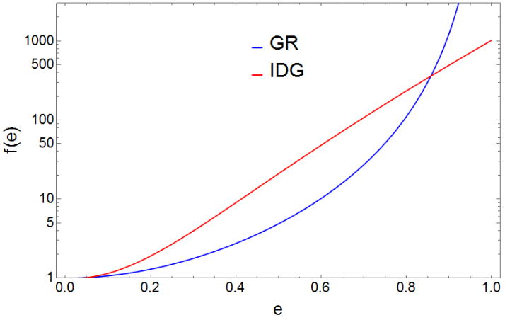
Figure 1: The enhancement factor $f^{\text{IDG}}(e)$ given by (32) against the eccentricity $e$ as well as the enhancement factor for the GR term $f^{\text{GR}}(e)$, where the total power is $P_{\text{GR}}^{\text{circ}}f^{\text{GR}}(e)+P_{\text{IDG}}^{\text{circ}}f^{\text{IDG}}(e)$. This factor describes how the power emitted changes with respect to the eccentricity. The extra IDG term will show up most strongly at around $e=0.7$, which coincidentally is close to the value for the Hulse-Taylor binary (0.617).

The power radiated by a binary system with a circular orbit is of limited applicability because in GR the power emitted is highly dependent on the eccentricity $e$ of the orbit Peters:1963ux , i.e. $P_{\text{GR}}=P_{\text{GR}}^{\text{circ}}f^{\text{GR}}(e)$. where $f^{\text{GR}}(e)$ is an enhancement factor that reaches $10^{3}$ at $e=0.9$. The circular orbit is therefore unlikely to be an accurate approximation.

For an elliptical orbit, the relevant components of the reduced quadrupole moment are Peters:1963ux

$$J_{xx}=\mu d^{2}\left(\cos^{2}(\psi)-\frac{1}{3}\right),\quad J_{yy}=\mu d^{2}\left(\sin^{2}(\psi)-\frac{1}{3}\right),~{}~{}~{}~{}~{}~{}$$ (20)

where $\mu$ is the reduced mass $m_{1}m_{2}/(m_{1}+m_{2})$ and the distance $d$ between the two bodies is given by
$d=\frac{a(1-e^{2})}{1+e\cos(\psi)}$, where $e$ is the eccentricity of the orbit and $a$ is the semimajor axis Peters:1963ux . The change in angular position over time is

$$\dot{\psi} = \frac{\left[G(m_{1}+m_{2})a(1-e^{2})\right]^{1/2}}{d^{2}}.$$ (21)

For the $xx$ component, we need to calculate

$$\hat{J}_{xx}=\mu a^{2}(1-e^{2})^{2}\int^{\infty}_{-\infty}dt^{\prime}_{r}e^{-M^{2}(t_{r}-t^{\prime}_{r})^{2}}\frac{\cos^{2}(\psi(t^{\prime}_{r}))-\frac{1}{3}}{\left(1+e\cos(\psi(t^{\prime}_{r}))\right)^{2}}.~{}~{}~{}~{}~{}~{}$$ (22)

This is a very difficult integration to do. However, if we make the change of coordinates $z=M(t_{r}-t^{\prime}_{r})$, we can use a Taylor expansion in $\frac{1}{M}$ if it is small and the identities (30) to see that we can write down (31), i.e.

$$P\approx P_{\text{GR}}+P_{\text{IDG}}=P_{\text{GR}}^{\text{circ}}f^{\text{GR}}(e)+P_{\text{IDG}}^{\text{circ}}f^{\text{IDG}}(e),~{}~{}~{}$$ (23)

where the IDG power for an elliptical orbit is the power for a circular orbit multiplied by an enhancement factor $f(e)$ which depends on the eccentricity.

We find that

$$P_{\text{IDG}}=P_{\text{IDG}}^{\text{circ}}f^{\text{IDG}}(e)=\frac{256}{5}\frac{\omega^{8}}{M^{2}}GR^{2}M_{s}^{4}f^{\text{IDG}}(e),~{}~{}~{}$$ (24)

where $f^{\text{IDG}}(e)$ is a polynomial of 22nd order and so is given in the appendix. In the limit $M\to\infty$, $P_{\text{IDG}}\to 0$ and (23) returns to $P_{\text{GR}}$. $f^{\text{IDG}}(e)$ is plotted in Fig 1 with a comparison to the enhancement factor for GR, $f^{\text{GR}}(e)$.

The Hulse-Taylor binary has a period of 7.5 hours and ellipticity of 0.617. The radiation emitted from the Hulse-Taylor binary is $0.998\pm 0.002$ of the GR prediction Weisberg:2016jye , which leads to the constraint $M>6.9\times 10^{-49}M_{P}=1.0\times 10^{-21}\text{eV}$ on our mass scale $M$, which is much weaker than previous constraints.

The previous lower bound is $\sim$0.01 eV from lab-based experiments Edholm:2016hbt . In order to produce a comparable constraint, we would need to study radiation produced from systems with orbital periods of less than $10^{-4}$ seconds. Not only do these systems have an orbital frequency much higher than LIGO and LISA will be able to probe (15-150 Hz Abbott:2016bqf and $10^{-4}$-$10^{-1}$ Hz Audley:2017drz respectively), but they would also be out of the weak-field regime we used for our calculations. Therefore lab-based experiments and CMB data are likely to provide the tightest constraints in the near future.

V Conclusion

We found the modified quadrupole formula for IDG, which describes how the metric changes for a given stress-energy tensor. We generalised the backreaction formula already found for Effective Quantum Gravity (EQG) to a de Sitter background (for both EQG and IDG). We used updated LIGO results to give a tighter constraint of $\epsilon<8.0\times 10^{-34}$ on the amplitude of the massive mode in EQG.

Finally, we found the power emitted by a binary system, for both circular and elliptical orbits and investigated the example of the Hulse-Taylor binary. We showed that IDG is consistent with the GR predictions.

VI Acknowledgements

We would like to thank David Burton, Iberê Kuntz and Sonali Mohapatra for their help in preparing this paper.

JE is funded by the Lancaster University Faculty of Science and Technology.

Appendix A Linearised and quadratic curvatures

The linearised Ricci curvatures around a de Sitter background are Conroy:2017uds

$$r^{\mu}_{\nu} = H^{2}h^{\mu}_{\nu}-\frac{1}{2}\Box h^{\mu}_{\nu},\quad\quad r=0.~{}~{}~{}~{}~{}~{}$$ (25)

The curvatures to quadratic order are

$$r^{(2)}_{\mu\nu} = \frac{1}{4}\left(h^{\alpha\beta}\nabla_{\mu}\nabla_{\nu}h_{\alpha\beta}-2h_{\alpha(\nu}(\Box-4H^{2})h^{\alpha}_{\mu)}\right)$$

$$r^{(2)} = -\frac{1}{4}h_{\mu\nu}\left(\Box-8H^{2}\right)h^{\mu\nu}.$$ (26)

The averaged second order equations of motion are

$$\kappa t^{\mu}_{\nu}{}^{\text{IDG}} = \frac{1}{2}\braket{h^{\mu}_{\sigma}F_{2}(\Box)\left(\Box-2H^{2}\right)^{2}h^{\sigma}_{\nu}}$$ (27)

$$-\frac{1}{8}\delta^{\mu}_{\nu}\braket{h^{\tau}_{\sigma}F_{2}(\Box)\left(\Box-2H^{2}\right)^{2}h^{\sigma}_{\tau}}.~{}~{}~{}~{}~{}~{}$$

Appendix B Adding a cosmological constant

It should be noted that it is possible to incorporate a cosmological constant $\Lambda$ to the linearised equations of motion by taking the “$\Lambda$-gauge” $\partial^{\nu}h_{\mu\nu}=\frac{1}{2}\partial_{\mu}h-\Lambda x_{\mu}$ Bernabeu:2011if . This adds an extra term $\Lambda h_{\mu\nu}$ onto the right hand side of (5). This gives us possibilities for future work.

Appendix C Other identities

We require the identities for integrating over a sphere Carroll:2004st

$$\int d\Omega=4\pi,\quad\int n_{i}n_{j}d\Omega=\frac{4\pi}{3}\delta_{ij},$$

$$\int n_{i}n_{j}n_{k}n_{l}d\Omega=\frac{4\pi}{15}\left(\delta_{ij}\delta_{kl}+\delta_{ik}\delta_{jl}+\delta_{il}\delta_{jk}\right),$$ (28)

Appendix D Elliptical orbits

Using our change of coordinates, the integral (22) becomes

$$\hat{J}_{xx}=-\frac{\mu}{M}\int^{-\infty}_{\infty}dz~{}e^{-z^{2}}\frac{\cos^{2}(\psi(t_{r}-\frac{z}{M}))-\frac{1}{3}}{\left(1+e\cos(\psi(t_{r}-\frac{z}{M}))\right)^{2}}.~{}~{}~{}~{}~{}~{}~{}$$ (29)

We can use a Taylor expansion in $\frac{1}{M}$ to write this as the GR expression $J_{xx}$ (the zeroeth order) plus the first order expression (which disappears as the integrand is odd) and finally the second order correction. We use the identities

$$\int^{-\infty}_{\infty} e^{-z^{2}}dz=-\sqrt{\pi},~{}~{}\quad\int^{-\infty}_{\infty}e^{-z^{2}}zdz=0,$$ (30)

$$~{}~{}~{}~{}\int^{-\infty}_{\infty}e^{-z^{2}}z^{2}dz=-\frac{\sqrt{\pi}}{2},$$

to find

$$\hat{J}_{xx} \approx J_{xx}-\frac{\sqrt{\pi}\mu}{24M^{2}(1+e\cos(\psi))^{4}}\bigg{\{}\psi^{\prime 2}\bigg{(}4\left(e^{2}-3\right)\cos(2\psi)-8e^{2}-19e\cos(\psi)+3e\cos(3\psi)\bigg{)}$$ (31)

$$-2\psi^{\prime\prime}\sin(\psi)\left(2\left(e^{2}+3\right)\cos(\psi)+e(3\cos(2\psi)+5)\right)\bigg{\}}~{}~{}~{}~{}~{}~{}$$

We perform a similar calculation for $\hat{J}_{yy}$ to find that the full enhancement factor for the IDG term $f^{\text{IDG}}(e)$ is given by

$$f(e)^{\text{IDG}} = 1-\frac{(9299+111168\pi)e}{12282+155520\pi}+\frac{(753298+4783383\pi)e^{2}}{18423+233280\pi}+\frac{(1347719-15413436\pi)e^{3}}{147384+1866240\pi}+\frac{(152362163+521885160\pi)e^{4}}{294768+3732480\pi}$$ (32)

$$-\frac{(6051611+36789444\pi)e^{5}}{72(2047+25920\pi)}+\frac{(666697961+1567922058\pi)e^{6}}{294768+3732480\pi}-\frac{15(1908618+1108133\pi)e^{7}}{32752+414720\pi}$$

$$+\frac{(344524449+556982911\pi)e^{8}}{65504+829440\pi}-\frac{(5826870871+2360357712\pi)e^{9}}{1152(2047+25920\pi)}+\frac{(37373085170+45561968109\pi)e^{10}}{4716288+59719680\pi}$$

$$-\frac{(45892881151+15257013132\pi)e^{11}}{6144(2047+25920\pi)}+\frac{(685593299971+742716547416\pi)e^{12}}{36864(2047+25920\pi)}-\frac{(18923346001+5812048566\pi)e^{13}}{2304(2047+25920\pi)}$$

$$+\frac{(1406663203279+1486964224080\pi)e^{14}}{73728(2047+25920\pi)}-\frac{(612225325649+186007875390\pi)e^{15}}{73728(2047+25920\pi)}$$

$$+\frac{(1879563787501+1982636168004\pi)e^{16}}{98304(2047+25920\pi)}-\frac{5(108886731499+33068066736\pi)e^{17}}{65536(2047+25920\pi)}$$

$$+\frac{(7518767717389+7930544672016\pi)e^{18}}{393216(2047+25920\pi)}-\frac{(9799832804557+2976126006240\pi)e^{19}}{1179648(2047+25920\pi)}$$

$$+\frac{(15037546015045+15861089344032\pi)e^{20}}{786432(2047+25920\pi)}+O(e^{21})$$

References

- [1] B. P. Abbott et al. Observation of Gravitational Waves from a Binary Black Hole Merger. Phys. Rev. Lett., 116(6):061102, 2016.
- [2] Joel M. Weisberg and Yuping Huang. Relativistic Measurements from Timing the Binary Pulsar PSR B1913+16. Astrophys. J., 829(1):55, 2016.
- [3] K. S. Stelle. Renormalization of higher-derivative quantum gravity. Phys. Rev. D, 16:953–969, Aug 1977.
- [4] Arkady A. Tseytlin. On singularities of spherically symmetric backgrounds in string theory. Phys. Lett., B363:223–229, 1995.
- [5] Tirthabir Biswas, Anupam Mazumdar, and Warren Siegel. Bouncing universes in string-inspired gravity. JCAP, 0603:009, 2006.
- [6] Tirthabir Biswas, Erik Gerwick, Tomi Koivisto, and Anupam Mazumdar. Towards singularity and ghost free theories of gravity. Phys. Rev. Lett., 108:031101, 2012.
- [7] Tirthabir Biswas, Alexey S. Koshelev, and Anupam Mazumdar. Gravitational theories with stable (anti-)de Sitter backgrounds. Fundam. Theor. Phys., 183:97–114, 2016.
- [8] W. Siegel. Stringy gravity at short distances. 2003.
- [9] Luca Buoninfante. Ghost and singularity free theories of gravity. 2016.
- [10] Spyridon Talaganis, Tirthabir Biswas, and Anupam Mazumdar. Towards understanding the ultraviolet behavior of quantum loops in infinite-derivative theories of gravity. Class. Quant. Grav., 32(21):215017, 2015.
- [11] Leonardo Modesto. Super-renormalizable Quantum Gravity. Phys. Rev., D86:044005, 2012.
- [12] Leonardo Modesto. Super-renormalizable Multidimensional Quantum Gravity. 2012.
- [13] James Edholm, Alexey S. Koshelev, and Anupam Mazumdar. Behavior of the Newtonian potential for ghost-free gravity and singularity-free gravity. Phys. Rev., D94(10):104033, 2016.
- [14] James Edholm and Aindriú Conroy. Newtonian Potential and Geodesic Completeness in Infinite Derivative Gravity. Phys. Rev., D96(4):044012, 2017.
- [15] James Edholm. Conditions for defocusing around more general metrics in Infinite Derivative Gravity. Phys. Rev., D97(8):084046, 2018.
- [16] Aindriu Conroy, Tomi Koivisto, Anupam Mazumdar, and Ali Teimouri. Generalized quadratic curvature, non-local infrared modifications of gravity and Newtonian potentials. Class. Quant. Grav., 32(1):015024, 2015.
- [17] Alan S. Cornell, Gerhard Harmsen, Gaetano Lambiase, and Anupam Mazumdar. Rotating metric in nonsingular infinite derivative theories of gravity. Phys. Rev., D97(10):104006, 2018.
- [18] Tirthabir Biswas, Aindriú Conroy, Alexey S. Koshelev, and Anupam Mazumdar. Generalized ghost-free quadratic curvature gravity. Class. Quant. Grav., 31:015022, 2014. [Erratum: Class. Quant. Grav.31,159501(2014)].
- [19] Gianluca Calcagni, Leonardo Modesto, and Piero Nicolini. Super-accelerating bouncing cosmology in asymptotically-free non-local gravity. Eur. Phys. J., C74(8):2999, 2014.
- [20] Tirthabir Biswas, Tomi Koivisto, and Anupam Mazumdar. Towards a resolution of the cosmological singularity in non-local higher derivative theories of gravity. JCAP, 1011:008, 2010.
- [21] Tirthabir Biswas, Alexey S. Koshelev, Anupam Mazumdar, and Sergey Yu. Vernov. Stable bounce and inflation in non-local higher derivative cosmology. JCAP, 1208:024, 2012.
- [22] Alexey S. Koshelev and Sergey Yu. Vernov. On bouncing solutions in non-local gravity. Phys. Part. Nucl., 43:666–668, 2012.
- [23] Alexey S. Koshelev. Stable analytic bounce in non-local Einstein-Gauss-Bonnet cosmology. Class. Quant. Grav., 30:155001, 2013.
- [24] Tirthabir Biswas, Alexey S. Koshelev, and Anupam Mazumdar. Consistent higher derivative gravitational theories with stable de Sitter and anti–de Sitter backgrounds. Phys. Rev., D95(4):043533, 2017.
- [25] Aindriú Conroy, Anupam Mazumdar, and Ali Teimouri. Wald Entropy for Ghost-Free, Infinite Derivative Theories of Gravity. Phys. Rev. Lett., 114(20):201101, 2015. [Erratum: Phys. Rev. Lett.120,no.3,039901(2018)].
- [26] James Edholm. UV completion of the Starobinsky model, tensor-to-scalar ratio, and constraints on nonlocality. Phys. Rev., D95(4):044004, 2017.
- [27] Fabio Briscese, Antonino Marcianò, Leonardo Modesto, and Emmanuel N. Saridakis. Inflation in (Super-)renormalizable Gravity. Phys. Rev., D87(8):083507, 2013.
- [28] Ali Teimouri, Spyridon Talaganis, James Edholm, and Anupam Mazumdar. Generalised Boundary Terms for Higher Derivative Theories of Gravity. JHEP, 08:144, 2016.
- [29] Alexey S. Koshelev, Leonardo Modesto, Leslaw Rachwal, and Alexei A. Starobinsky. Occurrence of exact inflation in non-local UV-complete gravity. JHEP, 11:067, 2016.
- [30] Ben Craps, Tim De Jonckheere, and Alexey S. Koshelev. Cosmological perturbations in non-local higher-derivative gravity. JCAP, 1411(11):022, 2014.
- [31] Spyridon Talaganis. Towards UV Finiteness of Infinite Derivative Theories of Gravity and Field Theories. 2017.
- [32] Aindriu Conroy, Alexey S. Koshelev, and Anupam Mazumdar. Geodesic completeness and homogeneity condition for cosmic inflation. Phys. Rev., D90(12):123525, 2014.
- [33] James Edholm. Revealing Infinite Derivative Gravity’s true potential: The weak-field limit around de Sitter backgrounds. Phys. Rev., D97(6):064011, 2018.
- [34] Joachim Naf and Philippe Jetzer. On Gravitational Radiation in Quadratic Gravity. Phys. Rev., D84:024027, 2011.
- [35] Sean M. Carroll. Spacetime and geometry: An introduction to general relativity. 2004.
- [36] Iberê Kuntz. Quantum Corrections to the Gravitational Backreaction. Eur. Phys. J., C78(1):3, 2018.
- [37] John F. Donoghue. The effective field theory treatment of quantum gravity. AIP Conf. Proc., 1483:73–94, 2012.
- [38] Xavier Calmet and Basem Kamal El-Menoufi. Quantum Corrections to Schwarzschild Black Hole. Eur. Phys. J., C77(4):243, 2017.
- [39] Xavier Calmet and Boris Latosh. Three Waves for Quantum Gravity. Eur. Phys. J., C78(3):205, 2018.
- [40] Leo C. Stein and Nicolas Yunes. Effective Gravitational Wave Stress-energy Tensor in Alternative Theories of Gravity. Phys. Rev., D83:064038, 2011.
- [41] Anthony W. H. Preston. Cosmological backreaction in higher-derivative gravity expansions. JCAP, 1608(08):038, 2016.
- [42] Keiki Saito and Akihiro Ishibashi. High frequency limit for gravitational perturbations of cosmological models in modified gravity theories. PTEP, 2013:013E04, 2013.
- [43] Yao-Dong Li, Leonardo Modesto, and Lesław Rachwał. Exact solutions and spacetime singularities in nonlocal gravity. JHEP, 12:173, 2015.
- [44] Aindriú Conroy. Infinite Derivative Gravity: A Ghost and Singularity-free Theory. PhD thesis, Lancaster U., 2017.
- [45] James Edholm and Aindriu Conroy. Criteria for resolving the cosmological singularity in Infinite Derivative Gravity around expanding backgrounds. Phys. Rev., D96(12):124040, 2017.
- [46] Breno L. Giacchini and Tibério de Paula Netto. Weak-field limit and regular solutions in polynomial higher-derivative gravities. 2018.
- [47] Jens Boos. Gravitational Friedel oscillations in higher-derivative and infinite-derivative gravity? 2018.
- [48] M. Nowakowski and I. Arraut. The Fate of a gravitational wave in de Sitter spacetime. Acta Phys. Polon., B41:911–925, 2010.
- [49] Ivan Arraut. About the propagation of the Gravitational Waves in an asymptotically de-Sitter space: Comparing two points of view. Mod. Phys. Lett., A28:1350019, 2013.
- [50] Xavier Calmet, Iberê Kuntz, and Sonali Mohapatra. Gravitational Waves in Effective Quantum Gravity. Eur. Phys. J., C76(8):425, 2016.
- [51] Xavier Calmet. The Lightest of Black Holes. Mod. Phys. Lett., A29(38):1450204, 2014.
- [52] X. Calmet, R. Casadio, A. Yu. Kamenshchik, and O. V. Teryaev. Graviton propagator, renormalization scale and black-hole like states. Phys. Lett., B774:332–337, 2017.
- [53] Xavier Calmet and Iberê Kuntz. Higgs Starobinsky Inflation. Eur. Phys. J., C76(5):289, 2016.
- [54] Benjamin P. Abbott et al. A Search for Tensor, Vector, and Scalar Polarizations in the Stochastic Gravitational-Wave Background. Phys. Rev. Lett., 120(20):201102, 2018.
- [55] Robert M. L. Baker. The Peoples Republic of China High-Frequency Gravitational Wave research program. AIP Conf. Proc., 1103:548–552, 2009.
- [56] P. C. Peters and J. Mathews. Gravitational radiation from point masses in a Keplerian orbit. Phys. Rev., 131:435–439, 1963.
- [57] P. A. R. Ade et al. Planck 2015 results. XIII. Cosmological parameters. Astron. Astrophys., 594:A13, 2016.
- [58] Benjamin P. Abbott et al. The basic physics of the binary black hole merger GW150914. Annalen Phys., 529(1-2):1600209, 2017.
- [59] Heather Audley et al. Laser Interferometer Space Antenna. 2017.
- [60] Jose Bernabeu, Domenec Espriu, and Daniel Puigdomenech. Gravitational waves in the presence of a cosmological constant. Phys. Rev., D84:063523, 2011. [Erratum: Phys. Rev.D86,069904(2012)].