Study and development of a Computer-Aided Diagnosis system for classification of chest x-ray images using convolutional neural networks pre-trained for ImageNet and data augmentation

Convolutional neural networks (ConvNets) are the actual standard for image recognizement and classification. On the present work we develop a Computer Aided-Diagnosis (CAD) system using ConvNets to classify a x-rays chest images dataset in two groups: Normal and Pneumonia. The study uses ConvNets models available on the PyTorch platform: AlexNet, SqueezeNet, ResNet and Inception. We initially use three training styles: complete from scratch using random initialization, using a pre-trained ImageNet model training only the last layer adapted to our problem (transfer learning) and a pre-trained model modified training all the classifying layers of the model (fine tuning). The last strategy of training used is with data augmentation techniques that avoid over fitting problems on ConvNets yielding the better results on this study.

1 Introduction

Computer-aided diagnosis (CAD) methods started on the 60’s[1] but without great success on that time. Large scale CAD usage arrived in the 80’s with the new approach of not replacing the medical professional but only assist in their diagnosis [2].

Recent growth of computational capacity allowed convolutional neural networks (ConvNets) applications on recognizement and detection of images to expand [3], this is true specially after the introduction of AlexNet in 2012 [4]. This growth also applies for CAD systems using ConvNets to classify patients.

Normally ConvNets can be subdivided in two networks. One network that extract features from the image, processing attributes like edges in a variety of orientations (e.g. horizontal or vertical ones) to form larger attributes of the images like the presence of square or rounded objects in it. The second network is the classifier that receives the features or attributes processed on the first layer and use all this information to classify the image in classes (i.e. groups of similar images). The process of training the network in extracting the features and classifying is a time-consuming one and demand a large dataset to get good features extracted instead of not so good ones.

To understand the problem of training those networks better the dataset for the ImageNet[5] competition have 1.000.000 images and even with this large dataset some networks seem to work better than others, even the same network can outperform itself due to a better training. In order to avoid this training problem two important techniques have emerged in reusing ConvNets for classification of small datasets:

Transfer Learning

is the method of using a network well trained on a similar task by copying its parameters and weights to the adapted network on the current task. Commonly we use the trained network only changing its final classifying layer or layers to solve the current task (e.g. removing the last layer outputting the 1.000 classes on ImageNet problem and adding one layer that outputs just 2 classes for our current problem). We can also handle this method by just adding an extra layer that will receive the original output and convert it to the current problem classes.

Data augmentation

is one of the techniques used on AlexNet [4] to improve its training and consist on geometric transformations that generates new training images from the original ones. Examples of those transformation can be doing an horizontal flip of the original images or just cropping and resizing it.

On the current task we will build a CAD system to classify x-rays chest images in two groups: Normal and Pneumonia, using ConvNets and comparing the performance using four different strategies:

Scratch

Networks initialized from scratch with random parameters, with no prior training.

Transfer Learning

Networks initialized with parameters copied from a network trained for ImageNet, replacing the final layers with new random initialized layers and only training those final layers.

Fine Tuning

Networks also initialized with parameters copied from ImageNet trained ones and with the final layer replaced but now training the classifier or even the entire network.

Data Augmentation

Networks trained with the same strategy as Fine Tuning but now with an augmented dataset, as explained later on.

2 Methodology

We used the PyTorch platform for all our neural network code since it replaced and also uses the code for the Caffe2 platform that was used by many other papers in this field.

The dataset used for our study can be found on [6] and was also used for an study in [7]. Some numbers on this dataset are on Table 2. On this study we only use the Test and Train sets ignoring the Validation set as it is too small and can’t provide a good estimative on the trained network quality or accuracy. The original images have different sizes but all way above the size normally used on ImageNet networks that is $224\times 224$.

Subset	Original	Balanced
Validation	23	16
Test	631	468
Train	5,223	2,682

Table 1: Number of chest x-rays images in the dataset from [6]

Network	Top-1	Top-5	Reference
Inception v3	22.55	6.44	[8]
ResNet 18	30.24	10.92	[9]
SqueezeNet 1.1	41.81	19.38	[10]
AlexNet	43.45	20.91	[4]

Table 2: List of the ConvNets used

We will use the ConvNets listed on Table 2 noting that in the initial phase of our study only some networks were used to minimize time spent on training.

The original dataset was unbalanced and for better usage we eliminated exceeding images from the Pneumonia class since it had the greater number. This was a random process made to have an 1:1 ratio between both Training and Test sets.

For the optimizer choice to train the network we made some simple tests with all the choices from PyTorch that had a simple and exchangeable operation on our code. The results can be seen on Fig. 1. Overall results are very similar on the long term and with exception of SGD we used the default parameters on the platform. We choose to use the Adam optimizer on the other tests since it showed the fastest convergence with higher accuracy and lower loss on the training set. Here is the full list of optimizers tested: a) ADADELTA[11] b) Adagrad[12] c) Adam[13] d) Adamax e) ASGD[14] f) RMSprop[15] g) Rprop h) SGD[16]

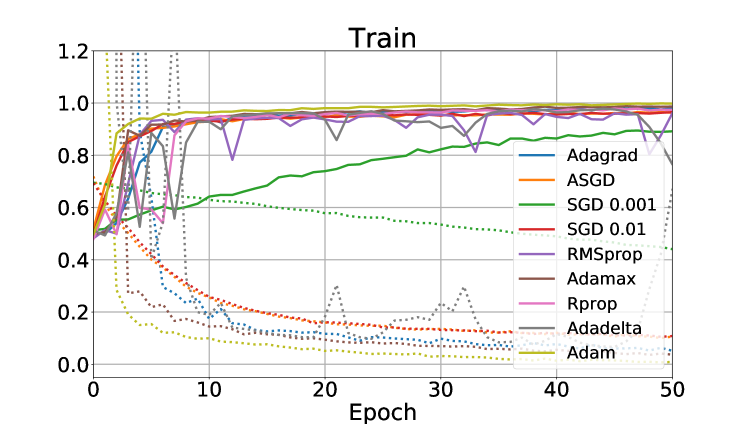
(a)

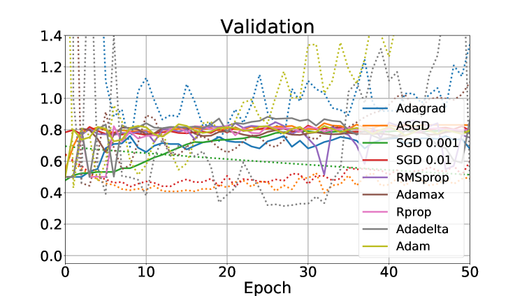
(b)

Figure 1: Optimizers comparison results using default parameters except where noted on SGD

For the transfer learning strategy we made some tests using the many methods seem on other studies, all on the AlexNet model:

• Adding an extra layer with 2 neurons connected to the 1.000 outputs of the original last layer, training only this extra layer.

• Changing the final layer of the original network so it only have 2 neurons getting in this way only 2 output classes, training only this final layer

• Change the entire AlexNet classifier network, diminishing the number of neurons on the hidden layers to analyse the impact on performance.

And for the fine tuning strategy:

• Changing the final layer on the original network to only have 2 output neurons but now training the entire classifier network.

In the data augmentation strategy we also used the fine tuning strategy by changing the final layer to get 2 output classes but now doing the data augmentation with the following methods from the PyTorch class torchvision.transforms:

transforms.RandomResizedCrop()

this method generates a new image by resizing and cropping the original image to the network input image size, using a random resize scale.

transforms.RandomHorizontalFlip()

this method will randomly do the horizontal flip on the image

3 Results

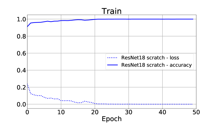
(a)

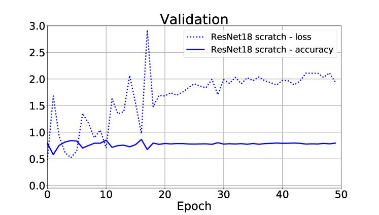
(b)

Figure 2: Training results of ResNet18 network from scratch

Using the ResNet18 network from scratch we got a maximum validation accuracy of $86.38\%$ (Fig. 2). As the epoch grows the training accuracy got to $100\%$ with its loss getting as low as $0.00034$ but without any reflex on the validation accuracy and a considerable growth in the validation loss. This is a possible evidence of over fitting where the network has adjusted too much to the training set using attributes irrelevant to our classification problem since it didn’t help the validation accuracy to increase. Similar results occurred with other networks used in the same strategy.

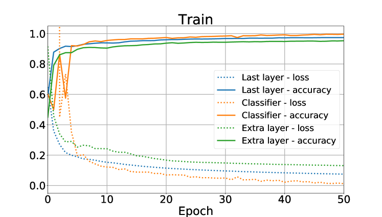
(a)

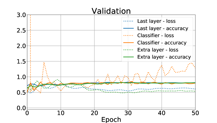
(b)

Figure 3: Transfer Learning results using the AlexNet network

Using the AlexNet network with the transfer learning strategy the accuracy gets a little better than the previous strategy but not all the tests made could reduce the training loss. This shows a limitation on the capacity of a single layer to classify our problem.

Only with fine tuning when we trained all the classifier network of the AlexNet network we could eliminate the training loss, but in this case we could also see some over fitting on the validation loss. The general validation accuracy of the three approaches to transfer learning where similar as can be seen on Fig. 3.

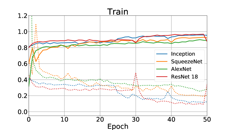
(a)

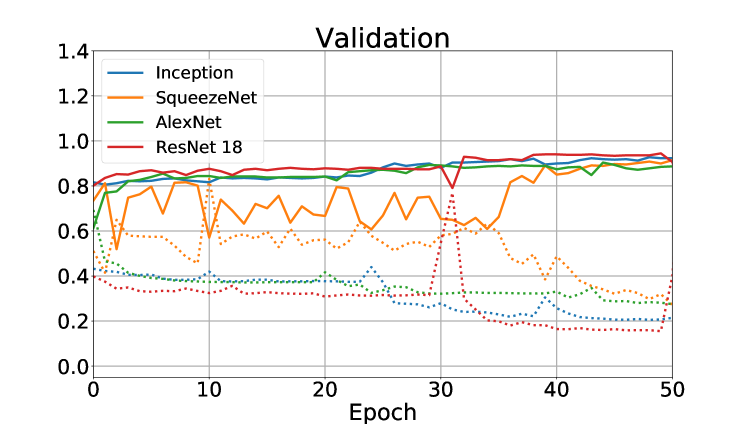
(b)

Figure 4: Training results of ConvNets using data augmentation - solid lines are accuracy and dotted lines loss

The best results in accuracy came from the transfer learning technique with data augmentation, as can be seen on Fig. 4. The data augmentation technique reduced the over fitting effect on the validation loss and also did not allowed the network to come close to an $100\%$ training accuracy or simply minimized the training loss. This can be credited to the data augmentation not allowing the network to adjust itself to the training set since it’s now been changing by data augmentation on every iteration. The best results in terms of accuracy come from the ResNet18 ($96.37\%$) and the Inception ($95.51\%$).

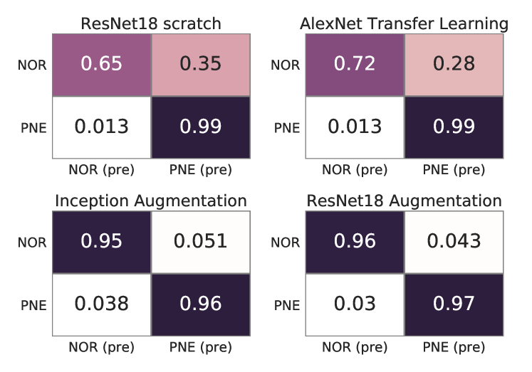
Figure 5: Confusion matrices - NOR stands for Normal, PNE for Pneumonia and (pre) means predicted

Fig. 5 shows the confusion matrices of different strategies used in this study, we can perceive a high number of false positives in networks without data augmentation (top matrices) even with a high number of hits in the Pneumonia class. When we use the data augmentation technique the false positive and false negative numbers dropped down (bottom matrices) with a high accuracy of both training and validation sets.

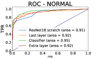
(a)

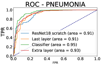
(b)

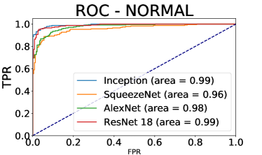
(c)

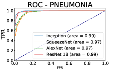
(d)

Figure 6: ROC curves for networks

Fig. 6 shows the ROC curves for the networks that explain better the selectivity of the classifiers. The confusion matrices shows that networks without data augmentation had a better accuracy on the Pneumonia class than the ones with data augmentation but now on the ROC curves we can see that this is not really the case. The data augmentation provided a better separation of the two classes making a more robust classifier reflecting on the ROC curves getting near the northwest corner of the graph.

4 Conclusions

It is possible and realistic to create a computer-aided diagnosis (CAD) system using ConvNets even with little computational resources for network training and a small dataset. In the better accuracy cases showed we only needed a few hours to complete the network training and some acceptable results even emerged on the first epochs of training.

To get a reliable CAD system it is convenient to rely on data augmentation techniques to avoid the over fitting problem of ConvNets. In the cases of large datasets maybe this may not be necessary but considering our current dataset of $2,682$ images data augmentation was necessary to get reliable results. One can even argument that the current dataset is not small since in the ImageNet case each class had $1,000$ images and they also used data augmentation techniques to improve the results in [4].

References

- [1] G. S. Lodwick et al. “COMPUTER DIAGNOSIS OF PRIMARY BONE TUMORS - A PRELIMINARY REPORT” In Radiology 80.2, 1963, pp. 273–275 DOI: 10.1148/80.2.273
- [2] K. Doi “Computer-aided diagnosis in medical imaging: Historical review, current status and future potential” In Computerized Medical Imaging and Graphics 31.4-5, 2007, pp. 198–211 DOI: 10.1016/j.compmedimag.2007.02.002
- [3] Y. LeCun, Y. Bengio and G. Hinton “Deep learning” In Nature 521.7553, 2015, pp. 436–444 DOI: 10.1038/nature14539
- [4] Alex Krizhevsky, Ilya Sutskever and Geoffrey E Hinton “ImageNet Classification with Deep Convolutional Neural Networks” In Advances in Neural Information Processing Systems 25 Curran Associates, Inc., 2012, pp. 1097–1105 URL: http://papers.nips.cc/paper/4824-imagenet-classification-with-deep-convolutional-neural-networks.pdf
- [5] Olga Russakovsky et al. “ImageNet Large Scale Visual Recognition Challenge” In International Journal of Computer Vision (IJCV) 115.3, 2015, pp. 211–252 DOI: 10.1007/s11263-015-0816-y
- [6] Daniel Kermany, Kang Zhang and Michael Goldbaum “Labeled Optical Coherence Tomography (OCT) and Chest X-Ray Images for Classification”, 2018 DOI: 10.17632/rscbjbr9sj.2
- [7] Daniel S. Kermany et al. “Identifying Medical Diagnoses and Treatable Diseases by Image-Based Deep Learning” In Cell 172.5 Elsevier, 2018, pp. 1122–1131.e9 DOI: 10.1016/j.cell.2018.02.010
- [8] Christian Szegedy et al. “Rethinking the Inception Architecture for Computer Vision” In CoRR abs/1512.00567, 2015 arXiv: http://arxiv.org/abs/1512.00567
- [9] Kaiming He, Xiangyu Zhang, Shaoqing Ren and Jian Sun “Deep Residual Learning for Image Recognition” In CoRR abs/1512.03385, 2015 arXiv: http://arxiv.org/abs/1512.03385
- [10] Forrest N. Iandola et al. “SqueezeNet: AlexNet-level accuracy with 50x fewer parameters and <1MB model size” In CoRR abs/1602.07360, 2016 arXiv: http://arxiv.org/abs/1602.07360
- [11] Matthew D. Zeiler “ADADELTA: An Adaptive Learning Rate Method” In CoRR abs/1212.5701, 2012 arXiv: http://arxiv.org/abs/1212.5701
- [12] John C. Duchi, Elad Hazan and Yoram Singer “Adaptive Subgradient Methods for Online Learning and Stochastic Optimization.” In Journal of Machine Learning Research 12, 2011, pp. 2121–2159 URL: http://dblp.uni-trier.de/db/journals/jmlr/jmlr12.html#DuchiHS11
- [13] Diederik P. Kingma and Jimmy Ba “Adam: A Method for Stochastic Optimization” In CoRR abs/1412.6980, 2014 arXiv: http://arxiv.org/abs/1412.6980
- [14] B. T. Polyak and A. B. Juditsky “Acceleration of Stochastic Approximation by Averaging” In SIAM J. Control Optim. 30.4 Philadelphia, PA, USA: Society for IndustrialApplied Mathematics, 1992, pp. 838–855 DOI: 10.1137/0330046
- [15] G. Hinton, Srivastava N. and K. Swesky “CSC321 - Introduction to Neural Networks and Machine Learning” Accessed: 2018-05-20, http://www.cs.toronto.edu/~tijmen/csc321/slides/lecture_slides_lec6.pdf
- [16] Ilya Sutskever, James Martens, George Dahl and Geoffrey Hinton “On the Importance of Initialization and Momentum in Deep Learning” In Proceedings of the 30th International Conference on International Conference on Machine Learning - Volume 28, ICML’13 Atlanta, GA, USA: JMLR.org, 2013, pp. III–1139–III–1147 URL: http://dl.acm.org/citation.cfm?id=3042817.3043064