IFUP–TH/2018          

We perform a systematic study of the modifications to the QCD vacuum energy density $\epsilon_{vac}$ in the zero-temperature case ($T=0$) caused by a small, but non-zero, value of the parameter $\theta$, using different effective Lagrangian models which include the flavour-singlet meson field and implement the $U(1)$ axial anomaly of the fundamental theory. In particular, we derive the expressions for the topological susceptibility $\chi$ and for the second cumulant $c_{4}$ starting from the $\theta$ dependence of $\epsilon_{vac}(\theta)$ in the various models that we have considered. Moreover, we evaluate numerically our results, so as to compare them with each other, with the predictions of the Chiral Effective Lagrangian, and, finally, also with the available lattice data.

1 Introduction

The discovery of instantons in the $70$’s [1] made clear that topology was a relevant aspect of the dynamics of the low-energy degrees of freedom in QCD [2, 3, 4], but it also raised another important issue: if one introduces in the QCD Lagrangian an additional term $\mathscr{L}_{\theta}=\theta Q$, where $Q(x)=\frac{g^{2}}{64\pi^{2}}\varepsilon^{\mu\nu\rho\sigma}F_{\mu\nu}^{a}(x)F_{\rho\sigma}^{a}(x)$ is the so-called topological charge density, despite the fact that $Q=\partial^{\mu}K_{\mu}$, where $K^{\mu}$ is the so-called Chern-Simons current, its contribution in the quantum theory would be non-zero thanks to the existence of configurations with non-trivial topology (such as instantons). This term, usually referred to as topological term or as $\theta$-term (from the name of the coefficient that appears in front of it), is particularly interesting since it introduces an explicit breaking of the CP symmetry in QCD (referred to as strong-CP violation), absent in the original theory. So far, however, no violation of the CP symmetry in strong interactions has been observed experimentally, so that the parameter $\theta$ is believed to be zero (or “practically” zero), despite the fact that it could assume, in principle, whatever value in $[0,2\pi)$. In particular, one can find a relation between the magnitude of the parameter $\theta$ and the neutron electric-dipole moment [5], $d_{N}\simeq\frac{M_{\pi}^{2}}{M_{N}^{3}}\,e\left|\theta\right|\simeq 10^{-16}\left|\theta\right|\;e\cdot cm$, where $M_{N}$ is the neutron mass, while $M_{\pi}$ is the pion mass. From the experimental data [6] we know that $d_{N}<10^{-26}e\cdot cm$, which leads to an upper bound:

$$\left|\theta\right|<10^{-10}.$$ (1.1)

(More refined relations among the neutron electric dipole moment and the $\theta$ angle were derived by Baluni [7], in the framework of the so-called bag model, by Crewther, Di Vecchia, Veneziano, and Witten [8], using the Chiral Perturbation Theory, and by many others using different approaches: see Sec. 7.1 of Ref. [9] for a more detailed discussion and also Ref. [10] for a recent lattice determination.)

This “fine-tuning” problem (usually referred to as the strong-CP problem), is still an open issue, despite possible solutions have been proposed (the most famous one being that of Peccei and Quinn [11], who proposed a mechanism, based on a new $U(1)$ symmetry and involving a new light pseudoscalar particle called axion [12], in order to dynamically rotate away the $\theta$-dependence of the theory).

However, it is nonetheless interesting to study the dependence of QCD on finite $\theta$: the insertion of the topological term with $\theta\neq 0$ in the QCD Lagrangian causes (by virtue of the non-trivial topology) a modification of the partition function of the theory and, therefore, a non-trivial dependence on $\theta$ of the vacuum energy density $\epsilon_{vac}(\theta)$, which will be the object of our investigations in this paper.

Let us write explicitly the expression for the partition function of the theory with $N_{f}$ quark flavours and with the inclusion of the $\theta$-term:

$$Z=\int[dA][d{}\mkern 2.0mu\overline{\mkern-2.0muq\mkern-2.0mu}\mkern 2.0mu{}dq]e^{i\int d^{4}x\mathscr{L}_{tot}},$$ (1.2)

where $\mathscr{L}_{tot}=-\frac{1}{2}\operatorname{Tr}\left[F_{\mu\nu}F^{\mu\nu}\right]+i{}\mkern 2.0mu\overline{\mkern-2.0muq\mkern-2.0mu}\mkern 2.0mu{}\gamma^{\mu}D_{\mu}q-{}\mkern 2.0mu\overline{\mkern-2.0muq\mkern-2.0mu}\mkern 2.0mu{}_{R}\mathcal{M}q_{L}-{}\mkern 2.0mu\overline{\mkern-2.0muq\mkern-2.0mu}\mkern 2.0mu{}_{L}\mathcal{M}^{\dagger}q_{R}+\theta Q$, with $\mathcal{M}$ a general complex mass matrix for the quarks. If we now perform a change of the (dummy) fermionic integration variables in (1.2) in the form of a $SU(N_{f})_{L}\otimes SU(N_{f})_{R}\otimes U(1)_{A}$ transformation,

$$\left\{\begin{aligned} q_{L}&\rightarrow q_{L}^{\prime}=\tilde{V_{L}}q_{L}=e^{i\alpha}V_{L}q_{L},\\ q_{R}&\rightarrow q_{R}^{\prime}=\tilde{V_{R}}q_{R}=e^{-i\alpha}V_{R}q_{R},\end{aligned}\right.$$ (1.3)

where $V_{L},~{}V_{R}\in SU(N_{f})$, we see that, because of the non-invariance of the fermionic functional-integral measure ($[d{}\mkern 2.0mu\overline{\mkern-2.0muq\mkern-2.0mu}\mkern 2.0mu{}dq]\rightarrow[d{}\mkern 2.0mu\overline{\mkern-2.0muq\mkern-2.0mu}\mkern 2.0mu{}^{\prime}dq^{\prime}]=[d{}\mkern 2.0mu\overline{\mkern-2.0muq\mkern-2.0mu}\mkern 2.0mu{}dq]e^{-i2L\alpha\int d^{4}x\,Q(x)}$) and of the mass term, the partition function $Z$ is invariant under the following changes:

$$\left\{\begin{aligned} \mathcal{M}&\rightarrow\mathcal{M}^{\prime}=\tilde{V}_{R}^{\dagger}\,\mathcal{M}\,\tilde{V}_{L},\\ \theta&\rightarrow\theta^{\prime}=\theta-2L\alpha.\end{aligned}\right.$$ (1.4)

We immediately notice that, if $\mathcal{M}$ is invertible ($\det\mathcal{M}\neq 0$), we have: $\arg(\det\mathcal{M}^{\prime})=\arg(\det\mathcal{M})+2L\alpha$, so that, under the transformation (1.3)-(1.4), the following combination:

$$\theta_{phys}\equiv\theta+\arg(\det\mathcal{M})$$ (1.5)

stays unchanged. This is the “physical” value of the parameter $\theta$: a non-zero value of $\theta_{phys}$ implies a strong CP-violation and the upper bound (1.1) actually refers to $\theta_{phys}$.

Eqs. (1.4) and (1.5) also imply that, if the mass matrix is invertible, then it is possible to move all the dependence on the parameter $\theta$ into the mass term. In fact, performing a transformation (1.3)-(1.4) with $\alpha=\frac{\theta}{2L}$, we obtain $\theta^{\prime}=0$ and $\arg(\det\mathcal{M}^{\prime})=\theta_{phys}$. On the other hand, if we take $\mathcal{M}$ to coincide with the physical quark-mass matrix $M\equiv\operatorname{diag}(m_{1},\ldots m_{N_{f}})$, with $m_{i}\in\mathbb{R}^{+}\;\forall i$ (which is always possible, by means of a transformation (1.3)-(1.4)), we have $\arg(\det M)=0$ and $\theta=\theta_{phys}$. (Of course, if at least one quark is massless, we have $\det{M}=0$ and, in this case, it is possible to rotate away all the dependence on $\theta_{phys}$ from the theory.)

From now on, we shall consider the partition function $Z[\theta]$ in this case ($\mathcal{M}=M$ and $\theta=\theta_{phys}$). In particular, we are interested in the $\theta$-dependence of the vacuum energy density $\epsilon_{vac}(\theta)$, which is related to the partition function $Z[\theta]$ by the following well-known relation:

$$Z[\theta]\equiv\frac{1}{\mathcal{N}}e^{-i\Omega\epsilon_{vac}(\theta)}\Rightarrow\epsilon_{vac}(\theta)=\frac{i}{\Omega}\log Z[\theta]+const.,$$ (1.6)

where $\mathcal{N}$ is a normalizing constant while $\Omega=VT$ is the four-volume considered (sending $\Omega\to\infty^{4}$ at the end). Being $\theta$ very small, it makes sense to Taylor-expand the vacuum energy density around $\theta=0$:

$$\epsilon_{vac}(\theta)=\epsilon_{vac}(0)+\frac{1}{2!}c_{2}\theta^{2}+\frac{1}{4!}c_{4}\theta^{4}+\ldots~{},~{}~{}~{}\text{with:}~{}~{}c_{n}\equiv\left.\frac{\partial^{n}\epsilon_{vac}(\theta)}{\partial\theta^{n}}\right|_{\theta=0}.$$ (1.7)

Only even powers of $\theta$ appear in (1.7) since the coefficients $c_{n}$ of the odd-power terms vanish by parity-invariance at $\theta=0$. The coefficients $c_{n}$ of this expansion are related to the correlation functions of the topological charge density at $\theta=0$. More explicitly, starting from the expression (1.6) and indicating with $Q_{tot}\equiv\int d^{4}x\,Q(x)$ the (total) topological charge, one easily finds that:

$$c_{2}\equiv\left.\frac{\partial^{2}\epsilon_{vac}(\theta)}{\partial\theta^{2}}\right|_{\theta=0}=-\frac{i}{\Omega}\langle Q_{tot}^{2}\rangle_{\theta=0}\equiv\chi,$$ (1.8)

i.e., the coefficient $c_{2}$ of the $\theta^{2}$ term in (1.7) coincides with the so-called topological susceptibility of the theory at $\theta=0$: $\chi\equiv-\frac{i}{\Omega}\langle Q_{tot}^{2}\rangle_{\theta=0}=-i\int d^{4}x\langle TQ(x)Q(0)\rangle_{\theta=0}$.

Concerning the coefficient $c_{4}$, it turns out to coincide with the second cumulant of the probability distribution of the topological charge-density operator $Q$ [9]:

$$c_{4}\equiv\left.\frac{\partial^{4}\epsilon_{vac}(\theta)}{\partial\theta^{4}}\right|_{\theta=0}=\frac{i}{\Omega}\left(\langle Q_{tot}^{4}\rangle_{\theta=0}-3\langle Q_{tot}^{2}\rangle^{2}_{\theta=0}\right),$$ (1.9)

which is related to the $\eta^{\prime}-\eta^{\prime}$ elastic scattering amplitude [4] and to the non-gaussianity of the topological charge distribution [9].

Therefore, the expansion (1.7) can be rewritten as:

$$\epsilon_{vac}(\theta)=\epsilon_{vac}(0)+\frac{1}{2}\chi\theta^{2}+\frac{1}{24}c_{4}\theta^{4}+\ldots$$ (1.10)

The strategy of this paper consists in computing the dependence on $\theta$ of the vacuum energy density, so as to obtain, exploiting the relations (1.8) and (1.9), the expressions of the topological susceptibility $\chi$ and of the second cumulant $c_{4}$ in terms of the fundamental parameters of the theory, not using directly the fundamental theory (which is anyhow possible using its formulation on the lattice: see the discussion in Sec. 6), but using some relevant effective Lagrangian models.

We shall first consider, in Sec. 2, the Chiral Effective Lagrangian in the case of $L$ ($\leq N_{f}$) light quark flavours (taken to be massless in the ideal chiral limit): the physically relevant cases are $L=2$, with the quarks $up$ and $down$, and $L=3$, including also the $strange$ quark [13, 14, 15, 16]. This effective theory describes the low-energy dynamics for the lightest hadronic states in the spectrum of QCD, i.e., the lightest non-flavour-singlet pseudoscalar mesons, which are identified with the $L^{2}-1$ pseudo-Goldstone bosons originated by the spontaneous breaking of the $SU(L)_{L}\otimes SU(L)_{R}$ chiral symmetry. The results that we shall report in Sec. 2 are already well known in the literature (see, in particular, Refs. [17, 18, 19, 20]). However, for the benefit of the reader, we have decided to report here some details of the calculations of $\chi$ and $c_{4}$ also in this case since this will allow us to introduce the basic notations and the main techniques for performing the calculations in the other cases. Moreover, this case is an important frame of reference for the other effective models that we shall discuss in the rest of the paper.

In Secs. 3 and 4 we shall consider different effective Lagrangian models which include the flavour-singlet meson field and also implement the $U(1)$ axial anomaly of the fundamental theory. In the last decades there were essentially two different “schools of thought” debating on how to address this issue: the first assumes that the dominant fluctuations are semiclassical instantons, while the second is based upon the large-$N_{c}$ limit of a $SU(N_{c})$ gauge theory, and assumes that the dominant fluctuations are not semiclassical but quantum. The two models that we shall consider in Secs. 3 and 4 belong respectively to the first trend (the so-called Extended (Non-)Linear sigma model [21, 22, 23]) and to the second one (the model of Witten, Di Vecchia, Veneziano, et al. [24, 25, 26]).

In Sec. 5, we shall consider another effective Lagrangian model (which was originally proposed in Refs. [27] and elaborated on in Refs. [28, 29, 30]), which is in a sense in-between the Extended (Non-)Linear sigma model and the model of Witten, Di Vecchia, Veneziano, et al.: for this reason we shall call it the Interpolating model.

Finally, in Sec. 6 we shall draw our conclusions, summarizing the analytical results that we have obtained for the topological susceptibility $\chi$ and the second cumulant $c_{4}$ in the four different frameworks mentioned above and also evaluating numerically our results, so as to critically compare them with each other and with the available lattice results.

2 The Chiral Effective Lagrangian

We first consider the Chiral Effective Lagrangian in the case of $L$ light quark flavours: the results that we shall report in this section are already well known in the literature (see, in particular, Refs. [17, 18, 19, 20]). However, for the benefit of the reader, we have decided to report here some details of the calculations of $\chi$ and $c_{4}$ also in this case since this will allow us to introduce the basic notations and the main techniques for performing the calculations in the other cases. Moreover, this case is an important frame of reference for all the other models that we shall discuss: in fact, if one “neglects” the presence of the flavour-singlet meson field and of the $U(1)$ axial anomaly (formally sending its mass to infinity), all the predictions derived in the other models must reduce to those that will be found in this section.

The chiral effective Lagrangian formulation was introduced by Weinberg [13] and was later elaborated on, becoming one of the most important tool to investigate the dynamics of the effective degrees of freedom of the low-energy regime of QCD [14, 15, 16]. The idea carried on by Weinberg et al. was that of building an effective theory for the lightest hadronic states in the spectrum of the theory, i.e., the lightest pseudoscalar mesons, which are the pseudo-Goldstone bosons originated by the spontaneous breaking of the chiral symmetry. This purpose can be achieved by writing down all the terms consistent with the symmetries of the fundamental theory, thereby obtaining an “exact” theory. However, the number of terms which satisfy the requirement is infinite: so, in order to be able to make any definite physical prediction, it is necessary to endow the theory with a power-counting ordering scheme which organizes the terms, providing a criterion to decide whether to keep or not a term at a given order. Such a criterion is the low-energy expansion, or the $p$-expansion: it consists in sorting the terms of the Chiral Effective Lagrangian on the basis of their number of derivatives, i.e., for the amplitudes in momentum space, on their order in the momentum-scale $p$. So, a generic Chiral Effective Lagrangian is written as:

$$\mathscr{L}_{eff}=\mathscr{L}_{eff}^{(0)}+\mathscr{L}_{eff}^{(2)}+\mathscr{L}_{eff}^{(4)}+\mathscr{L}_{eff}^{(6)}+\ldots,$$ (2.11)

where $\mathscr{L}_{eff}^{(2n)}$ gathers all the terms of order $p^{2n}$ (i.e, with $2n$ derivatives, the quark-mass matrix $\mathcal{M}$ counting as $p^{2}$, i.e., as two derivatives), while the odd-power terms are ruled out by Lorentz invariance. The term $\mathscr{L}_{eff}^{(0)}$ turns out to be an irrelevant constant, which can be neglected. In this paper, we shall make use of the Chiral Effective Lagrangian at the lowest (leading) nontrivial order $\mathcal{O}(p^{2})$. Here, we limit ourselves to report the final result (for a dissertation on the Chiral Effective Lagrangian up to the next-to-leading order $\mathcal{O}(p^{4})$, see Ref. [16]):

$$\mathscr{L}_{eff}^{(2)}(U,U^{\dagger})=\frac{1}{2}\operatorname{Tr}[\partial_{\mu}U\partial^{\mu}U^{\dagger}]+\frac{B_{m}}{2\sqrt{2}}\operatorname{Tr}\left[\mathcal{M}U+\mathcal{M}^{\dagger}U^{\dagger}\right],$$ (2.12)

where:

• the field $U$, describing only the $L^{2}-1$ non-flavour-singlet pseudo-Goldstone bosons, is an element of the group $SU(L)$, up to a multiplicative constant. In other words, it can be written as:

  $$U\equiv\frac{F_{\pi}}{\sqrt{2}}\,U^{\prime}~{},~{}~{}~{}U^{\prime}\in SU(L),$$ (2.13)

  where $F_{\pi}$ is the usual pion decay constant;

• $\mathcal{M}$ is a complex quark-mass matrix, which, considering the relation (1.5) between the coefficient $\theta$ of the topological term and the argument of the determinant of the mass matrix, can be taken to be:

  $$\mathcal{M}=Me^{i\frac{\theta_{phys}}{L}},$$ (2.14)

  where $M=\operatorname{diag}(m_{1},\ldots,m_{L})$ is the physical (real and diagonal) quark-mass matrix. In this way, we are moving all the dependence on $\theta_{phys}$ into the mass term. In order to simplify the notation, from now on we shall write $\theta$ in place of $\theta_{phys}$;

• $B_{m}$ is a constant having the dimension of an energy squared, often written as:

  $$B_{m}=2F_{\pi}B,$$ (2.15)

  where $B$ is a constant, carrying the dimension of an energy, which relates the mass of the quarks up and down to the mass of the pions through: $M_{\pi}^{2}=B(m_{u}+m_{d})$.

We can rewrite the Chiral Effective Lagrangian (2.12) as:

$$\mathscr{L}_{eff}^{(2)}(U,U^{\dagger})=\frac{1}{2}\operatorname{Tr}[\partial_{\mu}U\partial^{\mu}U^{\dagger}]-V(U,U^{\dagger}),$$ (2.16)

where the potential $V$ is given by:

$$V(U,U^{\dagger})=-\frac{B_{m}}{2\sqrt{2}}\operatorname{Tr}\left[\mathcal{M}U+\mathcal{M}^{\dagger}U^{\dagger}\right]=-\frac{B_{m}}{\sqrt{2}}\operatorname{Re}\left[\operatorname{Tr}\left(Me^{i\theta/L}U\right)\right].$$ (2.17)

We shall use the fact that (up to an irrelevant constant with respect to $\theta$), the vacuum energy density $\epsilon_{vac}(\theta)$ coincides with the minimum of the potential $V$ obtained with a configuration of fields constant with respect to space-time coordinates $x$ (see Refs. [17, 31] and references therein):

$$\epsilon_{vac}(\theta)\simeq V_{min}(\theta)+const.$$ (2.18)

Given that we are considering $M=\operatorname{diag}(m_{1},\ldots,m_{L})$, it is reasonable to look for the minimum of the potential guessing a configuration of the field $U$ in a diagonal form. So, being, in this case, $U=\frac{F_{\pi}}{\sqrt{2}}\,U^{\prime}$, where $U^{\prime}$ is an element of $SU(L)$, we set:

$$U=\frac{F_{\pi}}{\sqrt{2}}\operatorname{diag}\left(e^{i\alpha_{1}},\ldots,e^{i\alpha_{L}}\right),$$ (2.19)

where the $\alpha_{j}$ are constant phases, satisfying the constraint:

$$\det U^{\prime}=e^{i\sum_{j}\alpha_{j}}=1\Longrightarrow\sum\limits_{j=1}^{L}\alpha_{j}=0.$$ (2.20)

Substituting the explicit expressions for $M$ and $U$ into Eq. (2.17), we find:

$$V=-\frac{F_{\pi}B_{m}}{2}\sum\limits_{j=1}^{L}m_{j}\cos\phi_{j},$$ (2.21)

where we have defined $\phi_{j}\equiv\frac{\theta}{L}+\alpha_{j}$. Starting from Eq. (2.20), we see that the phases $\phi_{j}$ must satisfy the constraint:

$$\sum\limits_{j=1}^{L}\phi_{j}=\sum\limits_{j=1}^{L}\left(\frac{\theta}{L}+\alpha_{j}\right)=\theta.$$ (2.22)

It is now more convenient to consider separately the special case $L=2$ and the more general case $L\geq 2$: in fact, the former can be easily solved exactly, for any values of $\theta$ and of the quark masses; on the contrary, the latter cannot be solved exactly (in “closed form”) in general, but only an approximate solution can be derived.

2.1 A special case: $L=2$

In this case, it is easy to find the explicit expressions of the phases $\phi_{1}$ and $\phi_{2}$ which minimize the potential (2.21), with the constraint (2.22):

$$\phi_{1}=\arctan\left(\frac{m_{2}\sin\theta}{m_{1}+m_{2}\cos\theta}\right)~{},~{}~{}~{}\phi_{2}=\theta-\phi_{1}.$$ (2.23)

Substituting (2.23) in (2.21), the following expression for the minimum of the potential is found:

$$V(\theta)=\epsilon_{vac}(\theta)=-\frac{F_{\pi}B_{m}}{2}\sqrt{m_{1}^{2}+m_{2}^{2}+2m_{1}m_{2}\cos\theta}.$$ (2.24)

In the end, we are able to find the expressions for the topological susceptibility $\chi$ and the second cumulant $c_{4}$ [17, 18, 19, 20]:

$$\chi=\left.\frac{\partial^{2}\epsilon_{vac}(\theta)}{\partial\theta^{2}}\right|_{\theta=0}=\frac{F_{\pi}B_{m}}{2}\left(\frac{1}{m_{1}}+\frac{1}{m_{2}}\right)^{-1},$$ (2.25)

$$c_{4}=\left.\frac{\partial^{4}\epsilon_{vac}(\theta)}{\partial\theta^{4}}\right|_{\theta=0}=-\frac{F_{\pi}B_{m}}{2}\left(\frac{1}{m_{1}^{3}}+\frac{1}{m_{2}^{3}}\right)\left(\frac{1}{m_{1}}+\frac{1}{m_{2}}\right)^{-4}.$$ (2.26)

2.2 The more general case: $L\geq 2$

In the more general case $L\geq 2$ it is not possible to find an exact analytical solution, as in the previous case. However, given that our final purpose is to obtain the expressions for $\chi$ and $c_{4}$, which are by definition evaluated at $\theta=0$, we can implement a Taylor expansion of the potential around $\theta=0$. If we set $\theta=0$, it is easy to show that the form of the field $U$ which minimizes the potential is $U=\frac{F_{\pi}}{\sqrt{2}}\mathbf{I}$. We can thus implement a Taylor expansion of the potential (2.21) considering both $\theta\ll 1$ and $\phi_{i}\ll 1$ $\forall i$. After some calculations, the following expression for the phases $\phi_{i}$ which minimize the potential (2.21), with the constraint (2.22), is found:

$$\phi_{i}=\frac{\bar{m}}{m_{i}}\theta+\frac{1}{6}\frac{\bar{m}}{m_{i}}\left[\left(\frac{\bar{m}}{m_{i}}\right)^{2}-\sum\limits_{j=1}^{L}\left(\frac{\bar{m}}{m_{j}}\right)^{3}\right]\theta^{3}+\mathcal{O}(\theta^{5}),$$ (2.27)

where we have defined:

$$\bar{m}\equiv\left(\sum\limits_{i=1}^{L}\frac{1}{m_{i}}\right)^{-1}.$$ (2.28)

Finally, inserting (2.27) in (2.21), we find:

$$V(\theta)=\epsilon_{vac}(\theta)=const.+\frac{1}{2}\left[\frac{F_{\pi}B_{m}\bar{m}}{2}\right]\theta^{2}+\frac{1}{24}\left[-\frac{F_{\pi}B_{m}\bar{m}}{2}\sum_{j=1}^{L}\left(\frac{\bar{m}}{m_{j}}\right)^{3}\right]\theta^{4}+\ldots$$ (2.29)

From this expression, we extract the final results for the topological susceptibility and for the second cumulant [17, 18, 19, 20]:

$$\chi=\frac{F_{\pi}B_{m}\bar{m}}{2}=\frac{F_{\pi}B_{m}}{2}\left(\sum\limits_{j=1}^{L}\frac{1}{m_{j}}\right)^{-1},$$ (2.30)

$$c_{4}=-\frac{F_{\pi}B_{m}\bar{m}}{2}\sum\limits_{j=1}^{L}\left(\frac{\bar{m}}{m_{j}}\right)^{3}=-\frac{F_{\pi}B_{m}}{2}\left(\sum\limits_{j=1}^{L}\frac{1}{m_{j}}\right)^{-4}\sum\limits_{j=1}^{L}\frac{1}{m_{j}^{3}}.$$ (2.31)

These expressions correctly reduce to (2.25)-(2.26) if the number of light flavours considered is set to $L=2$. In this respect, we want also to oberve that, if one of the quark masses, let’s say $m_{L}$, is much larger than the other masses $m_{1},\ldots,m_{L-1}$, we can formally take the limit $m_{L}\to\infty$ in the expressions (2.30) and (2.31) for $\chi^{(L)}$ and $c_{4}^{(L)}$, which then reduce to $\chi^{(L-1)}$ and $c_{4}^{(L-1)}$, respectively. In the real-world case, for example, the mass of the strange quark, $m_{s}$, is much larger than the masses $m_{u}$ and $m_{d}$ of the up and down quarks: for this reason, in Sec. 6 we shall evaluate numerically the expressions (2.30) and (2.31) both for the case $L=2$, with only the quarks up and down, and for the case $L=3$, where also the strange quark is taken into account.

2.3 Considerations on the results

We recall that, if at least one quark is massless, the partition function of the theory (and, so, the vacuum energy density) turns out to be independent of $\theta$: we thus expect that, being the topological susceptibility and the second cumulant derivatives of the vacuum energy density with respect to $\theta$, if we let one of the quark masses tend to zero, both $\chi$ and $c_{4}$ will tend to zero as well. It is easy to check that the expressions (2.30) and (2.31) satisfy this property; in fact, considering a certain quark mass, say $m_{i}$, tending to zero, we have:

$$\chi\simeq\frac{F_{\pi}B_{m}m_{i}}{2}~{},~{}~{}~{}c_{4}\simeq-\frac{F_{\pi}B_{m}m_{i}}{2}~{},~{}~{}~{}{\rm for}~{}~{}m_{i}\to 0.$$ (2.32)

Or, also, if we take $m_{1}=\ldots=m_{L}\equiv m$, we find that:

$$\chi\simeq\frac{F_{\pi}B_{m}m}{2L}~{},~{}~{}~{}c_{4}\simeq-\frac{F_{\pi}B_{m}m}{2L^{3}}~{},~{}~{}~{}{\rm for}~{}~{}m\to 0.$$ (2.33)

The result found for the topological susceptibility $\chi$ in this limit is in agreement with what predicted by the relevant (flavour-singlet) Ward-Takahashi identities [32].

In the next sections, we shall consider different effective Lagrangian models which include the flavour-singlet meson field and also implement the $U(1)$ axial anomaly of the fundamental theory. As we have said in the Introduction, in the last decades there were essentially two different “schools of thought” debating on how to address this issue: the first assumes that the dominant fluctuations are semiclassical instantons, while the second is based upon the large-$N_{c}$ limit of a $SU(N_{c})$ gauge theory, and assumes that the dominant fluctuations are not semiclassical but quantum. The model that we shall consider in Sec. 3 (the so-called Extended (Non-)Linear sigma model) belongs to the first trend, while the model of Witten, Di Vecchia, Veneziano, et al., that we shall consider in Sec. 4, belongs to the second one.

3 The “Extended (Non-)Linear sigma model”

The first effective Lagrangian model with the inclusion of the flavour-singlet meson field that we consider was originally proposed in Refs. [21] to study the chiral dynamics at $T=0$, and later used in many different contexts (e.g., at non-zero temperature, around the chiral transition): in particular, ’t Hooft (see Refs. [22, 23] and references therein) argued that it reproduces, in terms of an effective theory, the $U(1)$ axial breaking caused by instantons in the fundamental theory. For brevity, from now on we shall refer to it as the Extended Linear sigma ($EL_{\sigma}$) model. This model is described by the following Lagrangian:

$$\mathscr{L}(U,U^{\dagger})=\mathscr{L}_{0}(U,U^{\dagger})+\frac{B_{m}}{2\sqrt{2}}\operatorname{Tr}\left[\mathcal{M}U+\mathcal{M}^{\dagger}U^{\dagger}\right]+\mathscr{L}_{I}(U,U^{\dagger}),$$ (3.34)

where $\mathscr{L}_{0}(U,U^{\dagger})$ is the Lagrangian of the so-called Linear sigma model, originally proposed in Ref. [33] but later elaborated on and extended:

$$\begin{split}\mathscr{L}_{0}(U,U^{\dagger})&=\frac{1}{2}\operatorname{Tr}[\partial_{\mu}U\partial^{\mu}U^{\dagger}]-V_{0}(U,U^{\dagger}),\\ V_{0}(U,U^{\dagger})&=\frac{1}{4}\lambda_{\pi}^{2}\operatorname{Tr}[(UU^{\dagger}-\rho_{\pi}\mathbf{I})^{2}]+\frac{1}{4}\lambda_{\pi}^{{}^{\prime}2}\left[\operatorname{Tr}(UU^{\dagger})\right]^{2},\end{split}$$ (3.35)

while $\mathscr{L}_{I}(U,U^{\dagger})$ is the term which is claimed to describe, in terms of the effective variables, the $2L$-fermions interaction vertex generated by the instantons. Its form is:

$$\mathscr{L}_{I}(U,U^{\dagger})=\kappa(\det U+\det U^{\dagger}),$$ (3.36)

where $\kappa$ is a constant which (according to ’t Hooft) is expected to be proportional to the typical instanton factor $e^{-8\pi^{2}/g^{2}}$ [2]. In this model, the mesonic effective fields are represented by a $L\times L$ complex matrix $U_{ij}$ which can be written, in terms of the quark fields, as:

$$U_{ij}\sim{}\mkern 2.0mu\overline{\mkern-2.0muq\mkern-2.0mu}\mkern 2.0mu{}_{j}\left(\frac{1+\gamma_{5}}{2}\right)q_{i}={}\mkern 2.0mu\overline{\mkern-2.0muq\mkern-2.0mu}\mkern 2.0mu{}_{jR}q_{iL},$$ (3.37)

up to a multiplicative constant. Under a chiral transformation (1.3) the field $U$ transforms as:

$$U\rightarrow\tilde{V}_{L}U\tilde{V}_{R}^{\dagger},$$ (3.38)

and, as a consequence, the determinant of the field $U$ varies as:

$$\det U\rightarrow\det(\tilde{V}_{L})\det(\tilde{V}_{R})^{*}\det U.$$ (3.39)

Therefore, the term (3.36) is invariant under $SU(L)_{L}\otimes SU(L)_{R}\otimes U(1)_{V}$, while under a $U(1)_{A}$ transformation, $U\to e^{i2\alpha}U$, it varies as:

$$\kappa(\det U+\det U^{\dagger})\rightarrow\kappa(e^{i2L\alpha}\det U+e^{-i2L\alpha}\det U^{\dagger}).$$ (3.40)

When using this model in our work, we have found more convenient to set the mass matrix in the real diagonal form $M=\operatorname{diag}(m_{1},\ldots,m_{L})$, by performing a $U(1)_{A}$ rotation of the field $U$ with $\alpha=-\frac{\theta}{2L}$, that is:

$$U\rightarrow e^{-i\theta/L}\,U.$$ (3.41)

After this rotation, the Lagrangian (3.34) is modified as:

$$\mathscr{L}(U,U^{\dagger})=\mathscr{L}_{0}(U,U^{\dagger})+\frac{B_{m}}{2\sqrt{2}}\operatorname{Tr}\left[M(U+U^{\dagger})\right]+\kappa(e^{-i\theta}\det U+e^{i\theta}\det U^{\dagger}).$$ (3.42)

For what concerns the potential $V_{0}(U,U^{\dagger})$ appearing in Eq. (3.35), we remind that the parameter $\rho_{\pi}$ is responsible for the fate of the chiral symmetry $SU(L)_{L}\otimes SU(L)_{R}$. In particular, if (as it happens at $T=0$) $\rho_{\pi}>0$, then the vacuum expectation value ${}\mkern 2.0mu\overline{\mkern-2.0muU\mkern-2.0mu}\mkern 2.0mu{}$ of the mesonic field $U$ (i.e., the value of $U$ for which the potential is at the minimum) is (even in the chiral limit $M=0$) different from zero and of the form ${}\mkern 2.0mu\overline{\mkern-2.0muU\mkern-2.0mu}\mkern 2.0mu{}|_{\rho_{\pi}>0}=v\,\mathbf{I}$, meaning that the chiral symmetry is spontaneously broken down to the vectorial $SU(L)_{V}$ subgroup.

If we are interested in describing only the low-energy dynamics of the effective pseudoscalar degrees of freedom (that is, the Goldstone [or would-be-Goldstone] bosons), we can decouple the scalar massive fields by letting $\lambda_{\pi}^{2}\rightarrow\infty$: in fact, in this way, we are implementing the static limit for the scalar fields, giving them infinite mass. In this limit, looking at the potential term in (3.35), we are forcing the constraint $UU^{\dagger}=\rho_{\pi}\,\mathbf{I}\equiv\frac{F_{\pi}^{2}}{2}\,\mathbf{I}$, which implies $\operatorname{Tr}(UU^{\dagger})=const.$: therefore, the term proportional to $\lambda_{\pi}^{{}^{\prime}2}$ is just an irrelevant constant term, which can be dropped. So, we shall neglect the scalar degrees of freedom and consider:

$$U=\frac{F_{\pi}}{\sqrt{2}}\,U^{\prime}~{},~{}~{}~{}U^{\prime}\in U(L).$$ (3.43)

In this way, the Lagrangian of the model reduces to:

$$\mathscr{L}=\frac{1}{2}\operatorname{Tr}\left[\partial_{\mu}U\partial^{\mu}U^{\dagger}\right]-V(U,U^{\dagger}),$$ (3.44)

where the potential $V$ is (apart from a trivial constant):

$$V(U,U^{\dagger})=-\frac{B_{m}}{2\sqrt{2}}\operatorname{Tr}\left[M(U+U^{\dagger})\right]-\kappa(e^{-i\theta}\det U+e^{i\theta}\det U^{\dagger}).$$ (3.45)

For brevity, from now on we shall refer to it as the Extended Non-Linear sigma ($ENL_{\sigma}$) model. Setting $M$ in the usual diagonal form and $U$ as in (2.19) (but without the constraint (2.20) since now $U^{\prime}$ belongs to $U(L)$), we find:

$$V(\vec{\alpha})=-\frac{F_{\pi}B_{m}}{2}\sum\limits_{j=1}^{L}m_{j}\cos\alpha_{j}-2\kappa\left(\frac{F_{\pi}}{\sqrt{2}}\right)^{L}\cos\left(\theta-\sum\limits_{j=1}^{L}\alpha_{j}\right).$$ (3.46)

The minimization equation is, therefore:

$$\frac{\partial V(\vec{\alpha})}{\partial\alpha_{i}}=\frac{F_{\pi}B_{m}}{2}m_{i}\sin\alpha_{i}-2\kappa\left(\frac{F_{\pi}}{\sqrt{2}}\right)^{L}\sin\left(\theta-\sum\limits_{j=1}^{L}\alpha_{j}\right)=0.$$ (3.47)

Again (as in the previous section), if we set $\theta=0$ the solution of the equation is $\alpha_{j}=0$ $\forall j$: we can thus consider both $\theta\ll 1$ and $\alpha_{j}\ll 1$ $\forall j$; moreover, from (3.46) we see that the change $\theta\rightarrow-\theta$ is equivalent to the change $\alpha_{j}\rightarrow-\alpha_{j}$ $\forall j$. Therefore we can expand the phases $\alpha_{j}$ in powers of $\theta$, as in the previous section, but keeping only the odd-power terms. So, we set:

$$\alpha_{i}=A_{i}\theta+C_{i}\theta^{3}+\ldots,$$ (3.48)

where the coefficients $A_{i}$ and $C_{i}$ have to be determined from the minimization condition. Inserting (3.48) in (3.47) and expanding up to $\theta^{3}$, we have:

$$\frac{\partial V(\vec{\alpha})}{\partial\alpha_{i}} =\left[\frac{F_{\pi}B_{m}m_{i}}{2}A_{i}-2\kappa\left(\frac{F_{\pi}}{\sqrt{2}}\right)^{L}\left(1-\sum_{j}A_{j}\right)\right]\theta$$ (3.49)

$$+\left[\frac{F_{\pi}B_{m}m_{i}}{2}\left(C_{i}-\frac{1}{6}A_{i}^{3}\right)+2\kappa\left(\frac{F_{\pi}}{\sqrt{2}}\right)^{L}\sum_{j}C_{j}\right.$$

$$\left.+2\kappa\left(\frac{F_{\pi}}{\sqrt{2}}\right)^{L}\frac{1}{6}\left(1-\sum_{j}A_{j}\right)^{3}\right]\theta^{3}+\ldots=0.$$

Requiring that these equalities are satisfied order by order in $\theta$, we derive the following expressions for the coefficients $A_{i}$ and $C_{i}$:

$$A_{i}=\frac{2\kappa\left(\frac{F_{\pi}}{\sqrt{2}}\right)^{L}}{\frac{F_{\pi}B_{m}\bar{m}}{2}+2\kappa\left(\frac{F_{\pi}}{\sqrt{2}}\right)^{L}}\,\frac{\bar{m}}{m_{i}},$$ (3.50)

$$C_{i}= \frac{1}{6}\frac{2\kappa\left(\frac{F_{\pi}}{\sqrt{2}}\right)^{L}}{\left(\frac{F_{\pi}B_{m}\bar{m}}{2}+2\kappa\left(\frac{F_{\pi}}{\sqrt{2}}\right)^{L}\right)^{4}}\,\frac{\bar{m}}{m_{i}}$$ (3.51)

$$\times \left\{\frac{F_{\pi}B_{m}\bar{m}}{2}\left[\left(2\kappa\left(\frac{F_{\pi}}{\sqrt{2}}\right)^{L}\right)^{2}\left(\frac{\bar{m}}{m_{i}}\right)^{2}-\left(\frac{F_{\pi}B_{m}\bar{m}}{2}\right)^{2}\right]\right.$$

$$+ \left.\left(2\kappa\left(\frac{F_{\pi}}{\sqrt{2}}\right)^{L}\right)^{3}\left[\left(\frac{\bar{m}}{m_{i}}\right)^{2}-\sum_{j}\left(\frac{\bar{m}}{m_{j}}\right)^{3}\right]\right\},$$

with $\bar{m}$ defined in Eq. (2.28). Substituting the form (3.48) in (3.46) and expanding up to the order $\theta^{4}$, we find:

$$V(\theta) =const.+\frac{1}{2}\left[\frac{F_{\pi}B_{m}}{2}\sum_{j}m_{j}A_{j}^{2}+2\kappa\left(\frac{F_{\pi}}{\sqrt{2}}\right)^{L}(1-\sum_{j}A_{j})^{2}\right]\theta^{2}$$ (3.52)

$$+\frac{1}{24}\left[24\frac{F_{\pi}B_{m}}{2}\sum_{j}m_{j}A_{j}C_{j}-\frac{F_{\pi}B_{m}}{2}\sum_{j}m_{j}A_{j}^{4}\right.$$

$$-\left.48\kappa\left(\frac{F_{\pi}}{\sqrt{2}}\right)^{L}(1-\sum_{j}A_{j})\sum_{j}C_{j}-2\kappa\left(\frac{F_{\pi}}{\sqrt{2}}\right)^{L}(1-\sum_{j}A_{j})^{4}\right]\theta^{4}+\ldots$$

Finally, substituting the relations (3.50) and (3.51) into (3.52), we can directly read, inside the square brackets, the expressions of the topological susceptibility and of the second cumulant. We report here the final results:

$$\chi=\frac{F_{\pi}B_{m}\bar{m}}{2}\frac{2\kappa\left(\frac{F_{\pi}}{\sqrt{2}}\right)^{L}}{\frac{F_{\pi}B_{m}\bar{m}}{2}+2\kappa\left(\frac{F_{\pi}}{\sqrt{2}}\right)^{L}}~{},$$ (3.53)

$$c_{4}= -\frac{F_{\pi}B_{m}\bar{m}}{2}\frac{2\kappa\left(\frac{F_{\pi}}{\sqrt{2}}\right)^{L}}{\left(\frac{F_{\pi}B_{m}\bar{m}}{2}+2\kappa\left(\frac{F_{\pi}}{\sqrt{2}}\right)^{L}\right)^{4}}$$ (3.54)

$$\times\left[\left(2\kappa\left(\frac{F_{\pi}}{\sqrt{2}}\right)^{L}\right)^{3}\sum_{j}\left(\frac{\bar{m}}{m_{j}}\right)^{3}+\left(\frac{F_{\pi}B_{m}\bar{m}}{2}\right)^{3}\right].$$

3.1 Considerations on the results

First of all, we notice that, if we take the (formal) limit $\kappa\rightarrow\infty$, the expressions for the topological susceptibility and for the second cumulant obtained in the $ENL_{\sigma}$ model reduce precisely to those found in the previous section using the Chiral Effective Lagrangian. To explain this fact, it is sufficient to observe that the flavour-singlet squared mass takes a contribution from the term proportional to $\kappa$ in the Lagrangian [see Eq. (3.36), which, using $U=({F_{\pi}}/{\sqrt{2}})U^{\prime}$ with $U^{\prime}=e^{i\sqrt{\frac{2}{L}}\frac{S_{\pi}}{F_{\pi}}}\tilde{U}^{\prime}$, $\tilde{U}^{\prime}\in SU(L)$, see Eq. (3.43), gives $M_{S_{\pi}}^{2}=\frac{2L}{F_{\pi}^{2}}2\kappa\left(\frac{F_{\pi}}{\sqrt{2}}\right)^{L}$ in the chiral limit of zero quark masses…] So, implementing the limit $\kappa\rightarrow\infty$, we are sending the flavour-singlet mass to infinity, decoupling it from the theory, which thus reduces to the Chiral Effective Lagrangian discussed in the previous section.

We also remark that (assuming that the parameter $\kappa$ is independent of the quark masses or, at least, that it has a finite non-vanishing value in the chiral limit) the expressions (3.53) and (3.54) have the right behaviour (2.32), in the chiral limit $m_{i}\to 0$, or (2.33), in the chiral limit $m_{1}=\ldots=m_{L}\equiv m\to 0$, as predicted by the relevant (flavour-singlet) Ward-Takahashi identities [32].

If, on the contrary, we take the infinite quark-mass limit, by sending all $m_{j}\rightarrow\infty$ (which results in $\bar{m}\rightarrow\infty$), we find that (assuming, again, that the parameter $\kappa$ is independent of the quark masses or, at least, that it has a finite, non-divergent value in the infinite quark-mass limit) the expressions (3.53) and (3.54) become:

$$\chi\to 2\kappa\left(\frac{F_{\pi}}{\sqrt{2}}\right)^{L}~{},~{}~{}~{}c_{4}\to-2\kappa\left(\frac{F_{\pi}}{\sqrt{2}}\right)^{L}.$$ (3.55)

In this way, we are implementing the static limit for the quarks, so that the theory should reduce to a pure Yang-Mills one. Indeed, the results (3.55) are in agreement with the $\theta$ dependence of the vacuum energy density expected in a pure-gauge theory as derived in an instanton-gas model [34]. In fact, in this case one finds that:

$$\epsilon_{vac}(\theta)\simeq\>const.-K\cos\theta=const.+\frac{1}{2}K\theta^{2}-\frac{1}{24}K\theta^{4}+\ldots,$$ (3.56)

that, by virtue of Eq. (1.10), leads to the relation $\chi=-c_{4}=K$, which, taking $K=2\kappa\left(\frac{F_{\pi}}{\sqrt{2}}\right)^{L}$, is satisfied by the results (3.55).

4 The effective Lagrangian model of Witten, Di Vecchia, Veneziano, et al.

A different chiral effective Lagrangian, with the inclusion of the flavour-singlet meson field, which implements the $U(1)$ axial anomaly of the fundamental theory, was proposed by Witten, Di Vecchia, Veneziano, et al. [24, 25, 26]: for brevity, in the following we shall refer to this model as the WDV model. Even if this model was derived and fully justified in the framework of the $1/N_{c}$ expansion (i.e., in the limit $N_{c}\rightarrow\infty$), the numerical results obtained using the $WDV$ model with $N_{c}=3$ are quite consistent with the real-world (experimental) values. This model is described by the Lagrangian (see Ref. [25] for a complete derivation):

$$\begin{split}\mathscr{L}(U,U^{\dagger},Q)&=\mathscr{L}_{0}(U,U^{\dagger})+\frac{B_{m}}{2\sqrt{2}}\operatorname{Tr}[M(U+U^{\dagger})]\\ &+\frac{i}{2}Q(x)\operatorname{Tr}\left[\log U-\log U^{\dagger}\right]+\frac{1}{2A}Q^{2}(x)+\theta Q(x),\end{split}$$ (4.57)

where $\mathscr{L}_{0}(U,U^{\dagger})$ is the Lagrangian of the Linear sigma model, reported in Eq. (3.35); $Q(x)$ is the topological charge density and is introduced here as an auxiliary field, while $A$ is a parameter which (at least in the large-$N_{c}$ limit) can be identified with the topological susceptibility in the pure Yang-Mills theory ($A=-i\int d^{4}x\langle TQ(x)Q(0)\rangle|_{YM}$). One immediately sees that the “anomalous” term $\mathscr{L}_{anom}\equiv\frac{i}{2}Q(x)\operatorname{Tr}\left[\log U-\log U^{\dagger}\right]$ in Eq. (4.57) is invariant under $SU(L)_{L}\otimes SU(L)_{R}\otimes U(1)_{V}$, while under a $U(1)_{A}$ transformation, $U\to e^{i2\alpha}U$, it transforms as:

$$\mathscr{L}_{anom}\rightarrow\mathscr{L}_{anom}-2L\alpha Q,$$ (4.58)

so correctly reproducing the $U(1)$ axial anomaly of the fundamental theory.

According to what one is investigating, it may be convenient to integrate out the auxiliary field $Q(x)$ using its equation of motion, i.e.,

$$Q(x)=-A\left[\theta+\frac{i}{2}\operatorname{Tr}\left(\log U-\log U^{\dagger}\right)\right].$$ (4.59)

After the substitution, we are left with:

$$\mathscr{L}(U,U^{\dagger})=\mathscr{L}_{0}(U,U^{\dagger})+\frac{B_{m}}{2\sqrt{2}}\operatorname{Tr}[M(U+U^{\dagger})]-\frac{A}{2}\left[\theta+\frac{i}{2}\operatorname{Tr}(\log U-\log U^{\dagger})\right]^{2}.$$ (4.60)

As we have done in the previous section for the $EL_{\sigma}$ model, we shall neglect the scalar degrees of freedom (retaining only the low-energy dynamics of the effective pseudoscalar degrees of freedom), by taking the formal limit $\lambda_{\pi}^{2}\rightarrow\infty$ (i.e., by taking the limit of infinite mass for the scalar fields), which, as we have shown, implies the constraint (3.43) for the matrix field $U$. In this way, the Lagrangian of the model reduces to:

$$\mathscr{L}=\frac{1}{2}\operatorname{Tr}\left[\partial_{\mu}U\partial^{\mu}U^{\dagger}\right]-V(U,U^{\dagger}),$$ (4.61)

where the potential $V$ is (apart from a trivial constant):

$$V(U,U^{\dagger})=-\frac{B_{m}}{2\sqrt{2}}\operatorname{Tr}\left[M(U+U^{\dagger})\right]+\frac{A}{2}\left[\theta+\frac{i}{2}\operatorname{Tr}(\log U-\log U^{\dagger})\right]^{2}.$$ (4.62)

Setting $M$ in the usual diagonal form and $U$ as in (2.19) (but without the constraint (2.20)), we find the following expression for the potential:

$$V(\vec{\alpha})=-\frac{F_{\pi}B_{m}}{2}\sum\limits_{j=1}^{L}m_{j}\cos\alpha_{j}+\frac{A}{2}\left(\theta-\sum\limits_{j=1}^{L}\alpha_{j}\right)^{2}.$$ (4.63)

Therefore, the minimization equation is:

$$\frac{\partial V(\vec{\alpha})}{\partial\alpha_{i}}=\frac{F_{\pi}B_{m}}{2}m_{i}\sin\alpha_{i}-A\left(\theta-\sum_{j}\alpha_{j}\right)=0.$$ (4.64)

As usual, since we are interested in the limit of small $\theta$ and, therefore, also of small phases $\alpha_{i}$ (in fact, $\theta=0$ implies that $\alpha_{i}=0$ $\forall i$), we can Taylor-expand the sine in Eq. (4.64) up to the third order in the phases:

$$\frac{\partial V(\vec{\alpha})}{\partial\alpha_{i}}\simeq\frac{F_{\pi}B_{m}}{2}m_{i}\left(\alpha_{i}-\frac{\alpha_{i}^{3}}{6}+\ldots\right)-A\left(\theta-\sum_{j}\alpha_{j}\right)=0,$$ (4.65)

and, moreover, observing that in (4.63) the change $\theta\rightarrow-\theta$ corresponds to the change $\alpha_{j}\rightarrow-\alpha_{j}$ $\forall j$, we can use for each phase $\alpha_{i}$ the following expansion in $\theta$:

$$\alpha_{i}=A_{i}\theta+C_{i}\theta^{3}+\ldots$$ (4.66)

Inserting the expressions (4.66) into Eq. (4.65), we find that:

$$\frac{\partial V(\vec{\alpha})}{\partial\alpha_{i}}(\theta) =\left[\frac{F_{\pi}B_{m}m_{i}}{2}A_{i}-A\left(1-\sum_{j}A_{j}\right)\right]\theta$$ (4.67)

$$+\left[\frac{F_{\pi}B_{m}m_{i}}{2}\left(C_{i}-\frac{1}{6}A_{i}^{3}\right)+A\sum_{j}C_{j}\right]\theta^{3}+\ldots=0.$$

Requiring that these equalities are satisfied order by order in $\theta$, we find the following expressions for the coefficients $A_{i}$ and $C_{i}$:

$$A_{i}=\frac{A}{\frac{F_{\pi}B_{m}\bar{m}}{2}+A}\frac{\bar{m}}{m_{i}},$$ (4.68)

$$C_{i}=\frac{1}{6}\left(\frac{A}{\frac{F_{\pi}B_{m}\bar{m}}{2}+A}\right)^{3}\frac{\bar{m}}{m_{i}}\left[\left(\frac{\bar{m}}{m_{i}}\right)^{2}-\frac{A}{\frac{F_{\pi}B_{m}\bar{m}}{2}+A}\sum_{j}\left(\frac{\bar{m}}{m_{j}}\right)^{3}\right],$$ (4.69)

with $\bar{m}$ defined in Eq. (2.28). Finally, Taylor-expanding the potential (4.63) up to the fourth order in the phases,

$$V(\vec{\alpha})\simeq const.+\frac{F_{\pi}B_{m}}{4}\sum\limits_{j=1}^{L}m_{j}\left(\bar{\alpha}_{j}^{2}-\frac{\bar{\alpha}_{j}^{4}}{12}+\ldots\right)+\frac{A}{2}\left(\theta-\sum\limits_{j=1}^{L}\bar{\alpha}_{j}\right)^{2},$$ (4.70)

and inserting the form (4.66), with the expressions (4.68) and (4.69) for the coefficients $A_{i}$ and $C_{i}$ into Eq. (4.70), we find:

$$V(\theta)= \>const.+\frac{1}{2}\chi\theta^{2}+\frac{1}{24}c_{4}\theta^{4}+\ldots,$$ (4.71)

with the following expressions for the topological susceptibility $\chi$ and the second cumulant $c_{4}$ in this model:

$$\chi=\frac{F_{\pi}B_{m}\bar{m}}{2}\frac{A}{\frac{F_{\pi}B_{m}\bar{m}}{2}+A},$$ (4.72)

$$c_{4}=-\frac{F_{\pi}B_{m}\bar{m}}{2}\left(\frac{A}{\frac{F_{\pi}B_{m}\bar{m}}{2}+A}\right)^{4}\sum\limits_{j=1}^{L}\left(\frac{\bar{m}}{m_{j}}\right)^{3}.$$ (4.73)

4.1 Considerations on the results

At first, we notice that the result (4.72) was already known in the literature [25], but it was obtained by studying the two-point correlation function of the topological charge density operator $Q(x)$ rather than by means of the $\theta$ expansion of the vacuum energy density; instead, for what concerns the result (4.73), it has been derived for the first time in this paper. If we consider the (formal) limit $A\rightarrow\infty$, the results (4.72)-(4.73) obtained in the $WDV$ model precisely reduce to those found in the framework of the Chiral Effective Lagrangian in Sec. 2. The reason is similar to the one discussed in the previous section for the $ENL_{\sigma}$ model: being the anomalous term proportional to $A$ in the Lagrangian (4.61)-(4.62) quadratic in the flavour-singlet field [using $U=({F_{\pi}}/{\sqrt{2}})U^{\prime}$ with $U^{\prime}=e^{i\sqrt{\frac{2}{L}}\frac{S_{\pi}}{F_{\pi}}}\tilde{U}^{\prime}$, $\tilde{U}^{\prime}\in SU(L)$, see Eq. (3.43), it gives $M_{S_{\pi}}^{2}=\frac{2LA}{F_{\pi}^{2}}$ in the chiral limit of zero quark masses …], such limit corresponds to send the flavour-singlet mass to infinity, decoupling it from the theory, which thus reduces to the SU(L) Chiral Effective Lagrangian discussed in Sec. 2.

For what concerns the topological susceptibility, we also observe that the result (4.72) coincides with the result (3.53) found in the $ENL_{\sigma}$ model provided that the following substitution is implemented:

$$A\longleftrightarrow 2\kappa\left(\frac{F_{\pi}}{\sqrt{2}}\right)^{L}.$$ (4.74)

And this correspondence also applies to the expression for the flavour-singlet squared mass $M_{S_{\pi}}^{2}$. Remarkably, this is not so for the second cumulant: indeed, even after such substitution, the result (4.73) does not turn into (3.54). This is due to the difference between the anomalous terms in Eqs. (4.62)-(4.63) and (3.45)-(3.46): while the anomalous term in Eqs. (4.62)-(4.63) is purely quadratic in the combination $\theta-\frac{\sqrt{2L}}{F_{\pi}}S_{\pi}$ (or: $\theta-\sum_{j}\alpha_{j}$), the anomalous term in Eqs. (3.45)-(3.46) is the cosine of such a combination.

We also remark that the expressions (4.72) and (4.73) have the right behaviour (2.32), in the chiral limit $m_{i}\to 0$, or (2.33), in the chiral limit $m_{1}=\ldots=m_{L}\equiv m\to 0$, as predicted by the relevant (flavour-singlet) Ward-Takahashi identities [32].

Instead, if we take the infinite quark-mass limit, by sending all $m_{j}\rightarrow\infty$ (which results in $\bar{m}\rightarrow\infty$), we find that:

$$\chi\to A~{},~{}~{}~{}c_{4}\to 0.$$ (4.75)

As we have already observed in the previous section, this limit is meant to “freeze” the dynamics of the quarks, reducing the model to a pure Yang-Mills one. So, we expect that in this limit the topological susceptibility coincides with that of the pure-gauge theory: it is exactly what happens in our case. For what concerns the second cumulant, it is null in this infinite quark-mass limit. This is due to the fact that the $WDV$ model is built considering only the leading terms in the expansion in $1/N_{c}$ and, so, while it contains the term $\frac{1}{2A}Q^{2}$ [see Eq. (4.57)], it does not contain also a term proportional to $Q^{4}$, which would contribute to the pure-gauge value of the second cumulant $c_{4}$: indeed, this kind of term is of the next-to-leading order in $1/N_{c}$ (for a detailed discussion on the next-to-leading terms, see Ref. [35]).

5 An “Interpolating model” with the inclusion of a U(1) axial condensate

In this section, we shall consider another effective Lagrangian model (which was originally proposed in Refs. [27] and elaborated on in Refs. [28, 29, 30]), which is in a sense in-between the $EL_{\sigma}$ model and the $WDV$ model: for this reason we shall call it the Interpolating model. Indeed, in this model the $U(1)$ axial anomaly is implemented, as in the $WDV$ model (4.57), by properly introducing the auxiliary field $Q$, so that it correctly satisfies the transformation property (4.58) under the chiral group. Moreover, it also includes an interaction term proportional to the determinant of the mesonic field $U$, which is similar to the interaction term (3.36) in the $EL_{\sigma}$ model, assuming that there is another $U(1)_{A}$-breaking condensate (in addition to the usual quark-antiquark chiral condensate $\langle\bar{q}q\rangle$). This extra $U(1)$ chiral condensate has the form $C_{U(1)}=\langle{\cal O}_{U(1)}\rangle$, where, for a theory with $L$ light quark flavors, ${\cal O}_{U(1)}$ is a $2L$-quark local operator that has the chiral transformation properties of [2, 36, 37] ${\cal O}_{U(1)}\sim\displaystyle{{\det_{st}}(\bar{q}_{sR}q_{tL})+{\det_{st}}(\bar{q}_{sL}q_{tR})}$, where $s,t=1,\dots,L$ are flavor indices. The color indices (not explicitly indicated) are arranged in such a way that (i) ${\cal O}_{U(1)}$ is a color singlet, and (ii) $C_{U(1)}=\langle{\cal O}_{U(1)}\rangle$ is a genuine $2L$-quark condensate, i.e., it has no disconnected part proportional to some power of the quark-antiquark chiral condensate $\langle\bar{q}q\rangle$; the explicit form of the condensate for the cases $L=2$ and $L=3$ is discussed in detail in the Appendix A of Ref. [29] (see also Ref. [38]).

The effective Lagrangian of the Interpolating model is written in terms of the topological charge density $Q$, the mesonic field $U_{ij}\sim\bar{q}_{jR}q_{iL}$ (up to a multiplicative constant), and the new field variable $X\sim{\det}\left(\bar{q}_{sR}q_{tL}\right)$ (up to a multiplicative constant), associated with the $U(1)$ axial condensate:

$$\begin{split}\mathscr{L}(U,U^{\dagger},X,&X^{\dagger},Q)=\frac{1}{2}\operatorname{Tr}[\partial_{\mu}U\partial^{\mu}U^{\dagger}]+\frac{1}{2}\partial_{\mu}X\partial^{\mu}X^{\dagger}\\ &-V_{0}(U,U^{\dagger},X,X^{\dagger})+\frac{i}{2}\omega_{1}Q(x)\operatorname{Tr}\left[\log U-\log U^{\dagger}\right]\\ &+\frac{i}{2}(1-\omega_{1})Q(x)\left[\log X-\log X^{\dagger}\right]+\frac{1}{2A}Q^{2}(x)+\theta Q(x),\end{split}$$ (5.76)

where

$$\begin{split}V_{0}(U,U^{\dagger},X,X^{\dagger})&=\frac{1}{4}\lambda_{\pi}^{2}\operatorname{Tr}[(UU^{\dagger}-\rho_{\pi}\mathbf{I})^{2}]+\frac{1}{4}\lambda_{\pi}^{{}^{\prime}2}\left[\operatorname{Tr}(UU^{\dagger})\right]^{2}\\ &+\frac{1}{4}\lambda_{X}^{2}[XX^{\dagger}-\rho_{X}]^{2}-\frac{B_{m}}{2\sqrt{2}}\operatorname{Tr}[M(U+U^{\dagger})]\\ &-\frac{\kappa_{1}}{2\sqrt{2}}[X^{\dagger}\det U+X\det U^{\dagger}].\end{split}$$ (5.77)

Since under a chiral $U(L)_{L}\otimes U(L)_{R}$ transformation (1.3) the field $X$ transforms exactly as $\det U$ [see Eq. (3.39)], i.e.,

$$X\rightarrow\det(\tilde{V}_{L})\det(\tilde{V}_{R})^{*}X,$$ (5.78)

[i.e., $X$ is invariant under $SU(L)_{L}\otimes SU(L)_{R}\otimes U(1)_{V}$, while, under a $U(1)$ axial transformation, $X\rightarrow e^{i2L\alpha}X$], we have that, in the chiral limit $M=0$, the effective Lagrangian (5.76) is invariant under $SU(L)_{L}\otimes SU(L)_{R}\otimes U(1)_{V}$, while under a $U(1)$ axial transformation, it correctly transforms as in Eq. (4.58).

As in the case of the $WDV$ model, the auxiliary field $Q(x)$ in (5.76) can be integrated out using its equation of motion:

$$Q(x)=-A\left\{\theta+\frac{i}{2}\left[\omega_{1}\operatorname{Tr}(\log U-\log U^{\dagger})+(1-\omega_{1})(\log X-\log X^{\dagger})\right]\right\}.$$ (5.79)

After the substitution, we obtain:

$$\mathscr{L}(U,U^{\dagger},X,X^{\dagger})=\frac{1}{2}\operatorname{Tr}[\partial_{\mu}U\partial^{\mu}U^{\dagger}]+\frac{1}{2}\partial_{\mu}X\partial^{\mu}X^{\dagger}-\tilde{V}(U,U^{\dagger},X,X^{\dagger}),$$ (5.80)

where

$$\begin{split}\tilde{V}(U,U^{\dagger}&,X,X^{\dagger})=V_{0}(U,U^{\dagger},X,X^{\dagger})\\ &+\frac{A}{2}\left\{\theta+\frac{i}{2}\left[\omega_{1}\operatorname{Tr}(\log U-\log U^{\dagger})+(1-\omega_{1})(\log X-\log X^{\dagger})\right]\right\}^{2}.\end{split}$$ (5.81)

Let us now briefly focus on the interaction term between $U$ and $X$ in Eqs. (5.76)-(5.77):

$$\mathscr{L}_{int}=\frac{\kappa_{1}}{2\sqrt{2}}[X^{\dagger}\det U+X\det U^{\dagger}].$$ (5.82)

This term has a form very similar to the “instantonic” term (3.36) of the $EL_{\sigma}$ model, but, differently from it, this term is invariant under the entire chiral group $U(L)_{L}\otimes U(L)_{R}$.

As usual, proceeding as we have done in the previous sections for the $EL_{\sigma}$ model and the $WDV$ model, we shall neglect the scalar degrees of freedom (retaining only the low-energy dynamics of the effective pseudoscalar degrees of freedom), by taking the formal limits $\lambda_{\pi}^{2}\rightarrow\infty$ and $\lambda_{X}^{2}\rightarrow\infty$ (i.e., by taking the limit of infinite mass for the scalar fields), which, in addition to the constraint (3.43) for the matrix field $U$, also implies the analogous constraint $XX^{\dagger}=\rho_{X}\equiv\frac{F_{X}^{2}}{2}$ for the $X$ field, i.e.,

$$X=\frac{F_{X}}{\sqrt{2}}\,e^{i\beta},$$ (5.84)

having introduced the decay constant $F_{X}$ of the field $X$, analogous to the decay constant $F_{\pi}$ of the pions. In this way, the Lagrangian of the model reduces to:

$$\mathscr{L}(U,U^{\dagger},X,X^{\dagger})=\frac{1}{2}\operatorname{Tr}[\partial_{\mu}U\partial^{\mu}U^{\dagger}]+\frac{1}{2}\partial_{\mu}X\partial^{\mu}X^{\dagger}-V(U,U^{\dagger},X,X^{\dagger}),$$ (5.85)

where the potential $V$ is (apart from a trivial constant):

$$V(U,U^{\dagger},X,X^{\dagger}) =-\frac{B_{m}}{2\sqrt{2}}\operatorname{Tr}[M(U+U^{\dagger})]-\frac{\kappa_{1}}{2\sqrt{2}}[X^{\dagger}\det U+X\det U^{\dagger}]$$ (5.86)

$$+\frac{A}{2}\left\{\theta+\frac{i}{2}\left[\omega_{1}\operatorname{Tr}(\log U-\log U^{\dagger})+(1-\omega_{1})(\log X-\log X^{\dagger})\right]\right\}^{2}.$$

Setting $M$ in the usual diagonal form, $U$ as in Eq. (2.19) (but without the constraint (2.20)) and the analogous parametrization (5.84) for the field $X$, where the phase $\beta$ (exactly as the phases $\alpha_{j}$) is constant with respect to $x$, we find the following expression for the potential:

$$V(\vec{\alpha},\beta)= -\frac{F_{\pi}B_{m}}{2}\sum\limits_{j=1}^{L}m_{j}\cos\alpha_{j}-c\cos\left(\beta-\sum\limits_{j=1}^{L}\alpha_{j}\right)$$ (5.87)

$$+\frac{A}{2}\left[\omega_{1}\sum\limits_{j=1}^{L}\alpha_{j}+(1-\omega_{1})\beta-\theta\right]^{2},$$

where we have defined:

$$c\equiv\kappa_{1}\frac{F_{X}}{2}\left(\frac{F_{\pi}}{\sqrt{2}}\right)^{L}.$$ (5.88)

In order to find the minimum of the potential, we have to solve the following system of minimization equations:

$$\frac{\partial V(\vec{\alpha},\beta)}{\partial\alpha_{i}}=0\quad\forall i=1,\ldots,L~{},~{}~{}~{}\frac{\partial V(\vec{\alpha},\beta)}{\partial\beta}=0,$$ (5.89)

which, after a slight rearrangement, read as follows:

$$\left\{\begin{aligned} &\frac{F_{\pi}B_{m}}{2}m_{i}\sin\alpha_{i}+A\left[\omega_{1}\sum\limits_{j=1}^{L}\alpha_{j}+(1-\omega_{1})\beta-\theta\right]=0,\\ \\ &c\sin\left(\beta-\sum_{j}\alpha_{j}\right)+A(1-\omega_{1})\left[\omega_{1}\sum\limits_{j=1}^{L}\alpha_{j}+(1-\omega_{1})\beta-\theta\right]=0.\end{aligned}\right.$$ (5.90)

It is easy to check that, in the case $\theta=0$, setting $\beta=0$ and $\alpha_{j}=0$ $\forall j$ puts the potential in its minimum. So, if we consider the case $\theta\ll 1$, we are allowed to use for the phases $\alpha_{i}$ and $\beta$ the following Taylor expansion in powers of $\theta$:

$$\alpha_{i}=A_{i}\theta+B_{i}\theta^{2}+C_{i}\theta^{3}+\ldots~{},~{}~{}~{}\beta=W\theta+Y\theta^{2}+Z\theta^{3}+\ldots$$ (5.91)

The coefficients $A_{i}$, $B_{i}$, $C_{i}$, $W$, $Y$, $Z$ have to be determined by solving (order by order in $\theta$) the system (5.90). Looking at the equations (5.90), it is easy to see that the change $\theta\rightarrow-\theta$ corresponds to the changes $\alpha_{j}\rightarrow-\alpha_{j}$ $\forall j$ and $\beta\rightarrow-\beta$, and, as a consequence, the coefficients of the even powers of $\theta$ in the expansions (5.91) must vanish:

$$Y=0~{},~{}~{}~{}B_{i}=0\quad\forall i.$$ (5.92)

Concerning the coefficients of the odd powers of $\theta$, the following expressions are found:

$$W=\frac{A\left[1+\frac{F_{\pi}B_{m}\bar{m}}{2c}(1-\omega_{1})\right]}{\frac{F_{\pi}B_{m}\bar{m}}{2}\left(1+\frac{A(1-\omega_{1})^{2}}{c}\right)+A},$$ (5.93)

$$A_{i}=\frac{A}{\frac{F_{\pi}B_{m}\bar{m}}{2}\left(1+\frac{A(1-\omega_{1})^{2}}{c}\right)+A}\frac{\bar{m}}{m_{i}},$$ (5.94)

$$Z= \frac{1}{6}\left(\frac{F_{\pi}B_{m}\bar{m}}{2}\right)A^{3}\left[\frac{F_{\pi}B_{m}\bar{m}}{2}\left(1+\frac{A(1-\omega_{1})^{2}}{c}\right)+A\right]^{-4}$$ (5.95)

$$\times\left[\left(\frac{F_{\pi}B_{m}\bar{m}}{2}\right)^{2}\frac{(1-\omega_{1})^{3}}{c^{3}}\left(\frac{F_{\pi}B_{m}\bar{m}}{2}+A\omega_{1}\right)\right.$$

$$+\left.\left(1-\frac{A\omega_{1}(1-\omega_{1})}{c}\right)\sum_{j}\left(\frac{\bar{m}}{m_{j}}\right)^{3}\right],$$

and:

$$C_{i}=\frac{1}{6} \left[\frac{A}{\frac{F_{\pi}B_{m}\bar{m}}{2}\left(1+\frac{A(1-\omega_{1})^{2}}{c}\right)+A}\right]^{3}\frac{\bar{m}}{m_{i}}$$ (5.96)

$$\times \left\{\left(\frac{\bar{m}}{m_{i}}\right)^{2}-\frac{A\left[\sum_{j}\left(\frac{\bar{m}}{m_{j}}\right)^{3}+\left(\frac{F_{\pi}B_{m}\bar{m}}{2c}\right)^{3}(1-\omega_{1})^{4}\right]}{\frac{F_{\pi}B_{m}\bar{m}}{2}\left(1+\frac{A(1-\omega_{1})^{2}}{c}\right)+A}\right\},$$

with $\bar{m}$ defined in Eq. (2.28). Substituting the expressions (5.91) (with $B_{i}=Y=0$) into Eq. (5.87) and expanding the potential up to the fourth order in $\theta$, we find:

$$V(\theta) \simeq const.{+}\frac{1}{2}\left\{\frac{F_{\pi}B_{m}}{2}\sum_{j}m_{j}A_{j}^{2}{+}c(W{-}\sum_{j}A_{j})^{2}{+}A\Big{[}\omega_{1}\sum_{j}A_{j}{+}(1{-}\omega_{1})W{-}1\Big{]}^{2}\right\}\theta^{2}$$ (5.97)

$${+}\frac{1}{24}\left\{24\,\frac{F_{\pi}B_{m}}{2}\sum_{j}m_{j}A_{j}C_{j}{-}\frac{F_{\pi}B_{m}}{2}\sum_{j}m_{j}A_{j}^{4}{+}24\,c\,(W{-}\sum_{j}A_{j})(Z{-}\sum_{j}C_{j})\right.$$

$$\left.{-}c\>(W{-}\sum_{j}A_{j})^{4}{+}24A\Big{[}\omega_{1}\sum_{j}A_{j}{+}(1{-}\omega_{1})W{-}1\Big{]}\Big{[}\omega_{1}\sum_{j}C_{j}{+}(1{-}\omega_{1})Z\Big{]}\right\}\theta^{4}+\ldots,$$

from which, after inserting the expressions (5.93)-(5.96), we obtain the following expressions for the topological susceptibility $\chi$ and the second cumulant $c_{4}$ in this model:

$$\chi=\frac{F_{\pi}B_{m}\bar{m}}{2}\>\frac{A}{\frac{F_{\pi}B_{m}\bar{m}}{2}\left(1+\frac{A(1-\omega_{1})^{2}}{c}\right)+A},$$ (5.98)

$$c_{4}=- \frac{F_{\pi}B_{m}\bar{m}}{2}\left[\frac{A}{\frac{F_{\pi}B_{m}\bar{m}}{2}\left(1+\frac{A(1-\omega_{1})^{2}}{c}\right)+A}\right]^{4}$$ (5.99)

$$\times\left[\sum\limits_{j=1}^{L}\left(\frac{\bar{m}}{m_{j}}\right)^{3}+\left(\frac{F_{\pi}B_{m}\bar{m}}{2c}\right)^{3}(1-\omega_{1})^{4}\right].$$

5.1 Considerations on the results

We first notice that the result (5.98) was originally found in Ref. [27], but once again it was obtained by a different approach, i.e., by directly studying the two-point function of the field $Q(x)$. On the contrary, the result (5.99) has been derived in this paper for the first time. Moreover, we notice that, if $\omega_{1}\neq 1$, the topological susceptibility obtained in this Interpolating model is smaller than the one obtained in the $WDV$ model, due to the positive (assuming $c>0$: see Refs. [29, 30]) corrective factor in the denominator. If, instead, we set $\omega_{1}=1$ (which, as we shall comment in the next section, represents the most natural choice at $T=0$) the results for both $\chi$ and $c_{4}$ coincide precisely with those of the $WDV$ model (independently of the other parameters $\kappa_{1}$ and $F_{X}$ of the model). The explanation of this fact lies in the potential (5.87): indeed, if we set $\omega_{1}=1$, we immediately see that, so as to obtain the minimum value for $V(\vec{\alpha},\beta)$, it is clear that we must set $\beta=\sum_{j}\alpha_{j}$, so that the cosine in the second term is equal to one. In this way, we find that the potential (5.87) coincides with the potential (4.63) of the $WDV$ model apart from a constant with respect to $\theta$: so, the final results for the topological susceptibility and for the second cumulant in the Interpolating model with $\omega_{1}=1$ are indeed expected to coincide with those of the $WDV$ model.

6 Conclusions: summary and analysis of the results

In this conclusive section, we shall summarize the analytical results that we have found for the topological susceptibility $\chi$ and the second cumulant $c_{4}$ in the various cases that we have considered. Moreover, we shall also report numerical estimates for these quantities, obtained both for $L=2$ and $L=3$ in the case of the Chiral Effective Lagrangian (see the discussion at the end of Sec. 2), and for $L=3$ in the other cases (effective Lagrangian models with the inclusion of the flavour-singlet meson field). For our numerical computations, the following values of the known parameters have been used:

• $A=\left(180\pm 5\;\text{MeV}\right)^{4}$ (see Ref. [39] and references therein).

• $F_{\pi}=92.2\pm 0.2$ MeV (see Ref. [40], where the value of $f_{\pi}=\sqrt{2}F_{\pi}$ is reported).

• For what concerns the parameter $B_{m}$, we shall rewrite it making use of the relation (2.15) in terms of the quantity $B$, which directly relates the quark masses to the light pseudoscalar meson masses. In particular, the following relations hold, at the leading order in the chiral perturbation theory:

  $$Bm_{u} =M_{\pi^{0}}^{2}-\frac{1}{2}\left(M_{K^{0}}^{2}-M_{K^{+}}^{2}+M_{\pi^{+}}^{2}\right),$$ (6.100)

  $$Bm_{d} =\frac{1}{2}\left(M_{K^{0}}^{2}-M_{K^{+}}^{2}+M_{\pi^{+}}^{2}\right),$$

  $$Bm_{s} =\frac{1}{2}\left(M_{K^{0}}^{2}+M_{K^{+}}^{2}-M_{\pi^{+}}^{2}\right).$$

  So, these expressions can be numerically evaluated using the known values for the masses of the mesons $\pi^{+}$, $\pi^{0}$, $K^{+}$, $K^{0}$ [40]:

  $$M_{\pi^{+}}=139.57061(24)\;\text{MeV},$$ (6.101)

  $$M_{\pi^{0}}=134.9770(5)\;\text{MeV},$$

  $$M_{K^{+}}=493.677(16)\;\text{MeV},$$

  $$M_{K^{0}}=497.611(13)\;\text{MeV}.$$

• For what concerns the quantity $\kappa$, its value is not known a priori. A possible way to evaluate it numerically is to make use of the relation among $\kappa$, $F_{\pi}$ and the meson masses, obtained within the $ENL_{\sigma}$ model in the case $L=3$:

  $$M^{2}_{\eta^{\prime}}+M^{2}_{\eta}-M_{K^{0}}^{2}-M_{K^{+}}^{2}=6\kappa\frac{F_{\pi}}{\sqrt{2}}.$$ (6.102)

  Substituting the experimental values of the meson masses (in addition to those given in (6.101) we need $M_{\eta}=547.862\pm 0.017$ MeV and $M_{\eta^{\prime}}=957.78\pm 0.06$ MeV [40]), we find for this parameter the value $\kappa=1856.38\pm 4.04$ MeV.

The values of all the parameters we listed above allow us to evaluate numerically all the results coming from the Chiral Effective Lagrangian at the leading order $\mathcal{O}(p^{2})$, the $ENL_{\sigma}$ model and the $WDV$ model. The situation of the Interpolating model is more complicated: due to the fact that very little is known about its peculiar parameters, it is not possible to give a complete numerical form to the results found in this model. In particular:

• For what concerns the parameter $F_{X}$, only an upper bound is known for it [27, 28, 29]: $\left|F_{X}\right|\leq 20$ MeV.

• For what concerns the parameter $\kappa_{1}$ (which was named “$c_{1}$” in the original papers), we cannot say too much, apart from the fact that (assuming $F_{X}\neq 0$) it cannot be zero (see Ref. [29] for a detailed discussion on the role of this parameter).

• At last, concerning the parameter $\omega_{1}$, we observe that the Lagrangian of the $WDV$ model is obtained from that of the Interpolating model by choosing $\omega_{1}=1$ (and then letting $F_{X}\to 0$). At low temperatures, one expects that the deviations from the $WDV$ Lagrangian are small, in some sense, and therefore that $\omega_{1}$ should not be much different from the unity near $T=0$ (on the other side, $\omega_{1}$ must necessarily be taken equal to zero above the chiral transition temperature, in order to avoid a singular behaviour of the anomalous term [27, 30]). Therefore, $\omega_{1}=1$ seems to be the most natural choice for $T=0$: with this choice, all the numerical values coincide with those of the $WDV$ model, regardless of the values of the other (unknown) parameters of the model, i.e., $\kappa_{1}$ and $F_{X}$.

Here is (in the following two subsections) a summary of both analytical and numerical results. [We recall that $\bar{m}$ is defined in Eq. (2.28).]

6.1 Topological susceptibility

• Chiral Effective Lagrangian $\mathcal{O}(p^{2})$:

  $$\chi= \frac{F_{\pi}B_{m}\bar{m}}{2}$$

  $$\chi^{(L=2)}= \left(77.25\pm 0.08\;\text{MeV}\right)^{4}$$

  $$\chi^{(L=3)}= \left(76.91\pm 0.08\;\text{MeV}\right)^{4}$$ (6.103)

• ENL_σ model:

  $$\chi= \frac{F_{\pi}B_{m}\bar{m}}{2}\frac{2\kappa\left(\frac{F_{\pi}}{\sqrt{2}}\right)^{L}}{\frac{F_{\pi}B_{m}\bar{m}}{2}+2\kappa\left(\frac{F_{\pi}}{\sqrt{2}}\right)^{L}}$$

  $$\chi^{(L=3)}= \left(76.271\pm 0.085\;\text{MeV}\right)^{4}$$ (6.104)

• WDV model:

  $$\chi= \frac{F_{\pi}B_{m}\bar{m}}{2}\frac{A}{\frac{F_{\pi}B_{m}\bar{m}}{2}+A}$$

  $$\chi^{(L=3)}= \left(76.283\pm 0.106\;\text{MeV}\right)^{4}$$ (6.105)

• Interpolating model:

  $$\chi= \frac{F_{\pi}B_{m}\bar{m}}{2}\>\frac{A}{\frac{F_{\pi}B_{m}\bar{m}}{2}\left(1+\frac{A(1-\omega_{1})^{2}}{c}\right)+A}$$

  $$\chi^{(L=3)}_{(\omega_{1}=1)}= \left(76.283\pm 0.106\;\text{MeV}\right)^{4}$$ (6.106)

6.2 Second cumulant

• Chiral Effective Lagrangian $\mathcal{O}(p^{2})$:

  $$c_{4}= -\frac{F_{\pi}B_{m}\bar{m}}{2}\sum\limits_{j=1}^{L}\left(\frac{\bar{m}}{m_{j}}\right)^{3}$$

  $$c_{4}^{(L=2)}= -\left(11.05\pm 0.49\right)\times 10^{6}\;\text{MeV}^{4}$$

  $$c_{4}^{(L=3)}= -\left(10.30\pm 0.46\right)\times 10^{6}\;\text{MeV}^{4}$$ (6.107)

• ENL_σ model:

  $$c_{4}= -\frac{F_{\pi}B_{m}\bar{m}}{2}\frac{2\kappa\left(\frac{F_{\pi}}{\sqrt{2}}\right)^{L}}{\left(\frac{F_{\pi}B_{m}\bar{m}}{2}+2\kappa\left(\frac{F_{\pi}}{\sqrt{2}}\right)^{L}\right)^{4}}$$

  $$\times\left[\left(2\kappa\left(\frac{F_{\pi}}{\sqrt{2}}\right)^{L}\right)^{3}\sum_{j}\left(\frac{\bar{m}}{m_{j}}\right)^{3}+\left(\frac{F_{\pi}B_{m}\bar{m}}{2}\right)^{3}\right]$$

  $$c_{4}^{(L=3)}= -\left(9.007\pm 0.426\right)\times 10^{6}\;\text{MeV}^{4}$$ (6.108)

• WDV model:

  $$c_{4}= -\frac{F_{\pi}B_{m}\bar{m}}{2}\left(\frac{A}{\frac{F_{\pi}B_{m}\bar{m}}{2}+A}\right)^{4}\sum\limits_{j=1}^{L}\left(\frac{\bar{m}}{m_{j}}\right)^{3}$$

  $$c_{4}^{(L=3)}= -\left(9.030\pm 0.134\right)\times 10^{6}\;\text{MeV}^{4}$$ (6.109)

• Interpolating model:

  $$c_{4}= -\frac{F_{\pi}B_{m}\bar{m}}{2}\left(\frac{A}{\frac{F_{\pi}B_{m}\bar{m}}{2}\left(1+\frac{A(1-\omega_{1})^{2}}{c}\right)+A}\right)^{4}$$

  $$\times\left[\sum\limits_{j=1}^{L}\left(\frac{\bar{m}}{m_{j}}\right)^{3}+\left(\frac{F_{\pi}B_{m}\bar{m}}{2c}\right)^{3}(1-\omega_{1})^{4}\right]$$

  $$c_{4~{}(\omega_{1}=1)}^{(L=3)}= -\left(9.030\pm 0.134\right)\times 10^{6}\;\text{MeV}^{4}$$ (6.110)

Let us make some remarks on these results. We observe that, within the present accuracy, there are no significant numerical differences between the results found in the $ENL_{\sigma}$ model and those found in the $WDV$ model (or in the Interpolating model with $\omega_{1}=1$), even if the theoretical expressions for the topological susceptibility and the second cumulant are in principle different (even considering the correspondence (4.74): see the discussion in Sec. 4.1). On the contrary, the numerical results found in the $ENL_{\sigma}$ model, the $WDV$ model, and the Interpolating model with $\omega_{1}=1$, are sensibly different from those found using the Chiral Effective Lagrangian at order $\mathcal{O}(p^{2})$. In this respect, we must here recall that in Refs. [18, 19, 20] also the non-leading order (NLO) correction to the result for the topological susceptibility using the Chiral Effective Lagrangian have been computed, and it turned out that it is of the order of percent for physical quark masses. Starting from our results, we can derive the order of the corrections caused by the presence of the flavour singlet to the numerical values obtained using the Chiral Effective Lagrangian $\mathcal{O}(p^{2})$, so as to make a comparison with that of the NLO corrections: for what concerns the topological susceptibility, these corrections are of the order of some percent and, so, are comparable with the NLO ones; for what concerns the second cumulant, instead, the corrections are considerably larger, being about the 12%.

6.3 Comparison of the results with the literature

In the end, let us make a comparison between the above-reported numerical estimates and the available lattice results in the literature. We first consider the topological susceptibility. The value of the topological susceptibility in full QCD has been measured through Monte Carlo simulations on the lattice. We report here two recent results, obtained with $L=2+1$ light flavours with physical quark masses:

$$\begin{split}\chi^{1/4}=73(9)\;\text{MeV}~{}\qquad\text{(see Ref. \cite[cite]{[\@@bibref{}{chi-lattice_1}{}{}]})};\\ \chi^{1/4}=75.6(2.0)\;\text{MeV}\quad\text{(see Ref. \cite[cite]{[\@@bibref{}{chi-lattice_2}{}{}]})},\end{split}$$ (6.111)

where, for the second value, the error in parentheses has been obtained adding in quadrature the statistical error (1.8) and the systematic error (0.9). These results are in perfect agreement (within the large errors) with all those found in our work. In figure 1, the numerical values obtained for the topological susceptibility in our work are reported together with the lattice results.

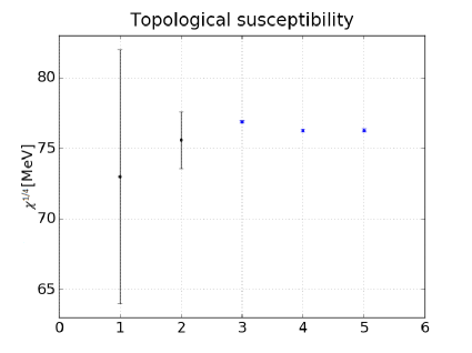
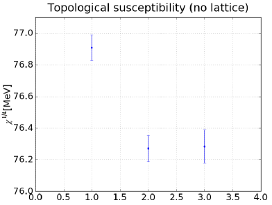
Figure 1: On the left, the two lattice results (6.111) for the topological susceptibility (in the full theory with quarks) and the three theoretical estimates for $L=3$, reported in Eqs. (• ‣ 6.1), (• ‣ 6.1), and (• ‣ 6.1)-(• ‣ 6.1), are shown (from left to right). On the right, only the three theoretical estimates are shown (in a different scale), so as to better compare them with each other.

With the help of this figure, we clearly see that the numerical value obtained using the Chiral Effective Lagrangian $\mathcal{O}(p^{2})$ (the first point in the figure on the right) is clearly detached from the ones related to the $ENL_{\sigma}$ model and to the $WDV$ (or Interpolating) model (respectively, the second and the third point in the figure on the right). Besides, these last two values are evidently compatible within the uncertainties.

Let us now move to the second cumulant. In lattice simulations, a quantity which is linked to the second cumulant is usually measured rather than the second cumulant itself, due to a simpler definition on the lattice. We report here the definition of this quantity, usually called $b_{2}$ (a more detailed description of this parameter can be found in Ref. [9]):

$$b_{2}\equiv\frac{c_{4}}{12\chi}=-\frac{\langle Q_{tot}^{4}\rangle_{\theta=0}-3\langle Q_{tot}^{2}\rangle^{2}_{\theta=0}}{12\langle Q_{tot}^{2}\rangle_{\theta=0}}.$$ (6.112)

All the lattice determinations of this parameter at $T=0$ are obtained, to date, in $SU(N_{c})$ pure-gauge frameworks, considering $N_{c}\geq 3$: it must be taken into account that our final results have been obtained in a full QCD framework. There are, in the literature, a number of results for $b_{2}$ at $N_{c}=3$, obtained using different approaches (see Ref. [9] and references therein):

$$b_{2} =-0.023(7)\quad\text{(cooling method)};$$ (6.113)

$$b_{2} =-0.024(6)\quad\text{(heating method)};$$

$$b_{2} =-0.025(9)\quad\text{(overlap method)};$$

while more recent results are:

$$\begin{split}b_{2}&=-0.026(3)\qquad\text{(see Ref. \cite[cite]{[\@@bibref{}{b2-lattice_1}{}{}]})};\\ b_{2}&=-0.0216(15)\quad\text{(see Ref. \cite[cite]{[\@@bibref{}{b2-lattice_2}{}{}]})}.\end{split}$$ (6.114)

Starting from our results for the topological susceptibility and for the second cumulant in the various cases described, we find:

• Chiral Effective Lagrangian $\mathcal{O}(p^{2})$:

  $$b_{2}^{(L=2)}= -0.026(1)$$

  $$b_{2}^{(L=3)}= -0.025(1)$$ (6.115)

• ENL_σ model:

  $$b_{2}^{(L=3)}=-0.0222(1)$$ (6.116)

• WDV model:

  $$b_{2}^{(L=3)}=-0.0222(4)$$ (6.117)

• Interpolating model:

  $$b_{2~{}(\omega_{1}=1)}^{(L=3)}=-0.0222(4)$$ (6.118)

In figure 2, these theoretical estimates for $b_{2}$ (for the full theory with $L=3$) are reported together with the above-mentioned lattice (pure-gauge) results.

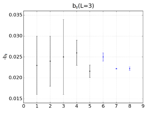
Figure 2: The five lattice (pure-gauge) results, reported in Eqs. (6.113) and (6.114), and the three theoretical estimates for the full theory with $L=3$, reported in Eqs. (• ‣ 6.3), (6.116), and (6.117)-(6.118), are shown (from left to right).

We notice that the lattice (pure-gauge) results turn out to be compatible (in almost all cases) with our theoretical estimates: this global accordance is quite impressive, considering that our results have been derived in full QCD rather than in a pure Yang-Mills theory. We also recall that, on the basis of the results obtained in Secs. 3.1, 4.1, and 5.1, the value of the ratio $b_{2}$ tends, in the infinite quark-mass limit, to the pure-gauge value $b_{2}^{(YM)}=-\frac{1}{12}\simeq-0.083$ (also obtained using a pure-gauge instanton-gas model) in the $ENL_{\sigma}$ model [see Eq. (3.55)], while it tends to the pure-gauge value $b_{2}^{(YM)}=0$ in the $WDV$ model (and in the Interpolating model with $\omega_{1}=1$) [see Eq. (4.75)]: therefore, we see that both the lattice pure-gauge data and our full-QCD theoretical estimates lie in between these two different values and (considering the errors) they disagree with both of them, even if they are considerably closer to the second one. It will be interesting to see if future more precise lattice data (including also the effects of quarks with physical masses) will confirm (or not) this curious coincidence.

References

- [1] A.A. Belavin, A.M. Polyakov, A.S. Schwartz, Y.S. Tyupkin, Phys. Lett. 59B, 85 (1975).
-
[2]
G. ’t Hooft, Phys. Rev. Lett. 37, 8 (1976);
G. ’t Hooft, Phys. Rev. D 14, 3432 (1976);
G. ’t Hooft, Phys. Rev. D. 18, 2199(E) (1978). - [3] E. Witten, Nucl. Phys. B156, 269 (1979).
- [4] G. Veneziano, Nucl. Phys. B159, 213 (1979).
- [5] S. Weinberg, The Quantum Theory of Fields, Vol.2: Modern Applications (Cambridge University Press, Cambridge, UK, 1995).
- [6] C.A. Baker, D.D. Doyle, P. Geltenbort, K. Green, M.G.D. van der Grinten, P.G. Harris, P. Iaydjiev, S.N. Ivanov, D.J.R. May, J.M. Pendlebury, J.D. Richardson, D. Shiers, K.F. Smith, et al., Phys. Rev. Lett. 97, 131801 (2006).
- [7] V. Baluni, Phys. Rev. D 19, 2227 (1979).
-
[8]
R.J. Crewther, P. Di Vecchia, G. Veneziano, E. Witten, Phys. Lett. 88B, 123 (1979);
R.J. Crewther, P. Di Vecchia, G. Veneziano, E. Witten, Phys. Lett. 91B, 487(E) (1980). - [9] E. Vicari, H. Panagopoulos, Phys. Rep. 470, 93 (2009).
- [10] F.-K. Guo et al., Phys. Rev. Lett. 115, 062001 (2015).
-
[11]
R.D. Peccei, H.R. Quinn, Phys. Rev. Lett. 38, 1440 (1977);
R.D. Peccei, H.R. Quinn, Phys. Rev. D 16, 1791 (1977). -
[12]
S. Weinberg, Phys. Rev. Lett. 40, 223 (1978);
F. Wilczek, Phys. Rev. Lett. 40, 279 (1978). - [13] S. Weinberg, Phys. Rev. Lett. 18, 188 (1967).
- [14] S. Weinberg, Physica 96A, 327 (1979).
-
[15]
J. Gasser, H. Leutwyler, Phys. Rept. 87C, 77 (1982);
J. Gasser, H. Leutwyler, Phys. Lett. 125B, 321 (1983);
J. Gasser, H. Leutwyler, Ann. Phys. 158, 142 (1984). - [16] J. Gasser, H. Leutwyler, Nucl. Phys. B250, 465 (1985).
- [17] A. Smilga, Lectures on Quantum Chromodynamics (World Scientific, Singapore, 2001).
- [18] Y. Mao, T. Chiu, Phys. Rev. D 80, 034502 (2009).
- [19] F.-K. Guo, U.-G. Meissner, Phys. Lett. B 749, 278 (2015).
- [20] G. Grilli di Cortona, E. Hardy, J.P. Vega, G. Villadoro, JHEP 01, 034 (2016).
-
[21]
M. Levy, Nuovo Cimento A 52, 23 (1967);
W.A. Bardeen, B.W. Lee, Phys. Rev. 177, 2389 (1969);
S. Gasiorowicz, D.A. Geffen, Rev. Mod. Phys. 41, 531 (1969). - [22] G. ’t Hooft, Phys. Rep. 142, 357 (1986).
- [23] G. ’t Hooft, The Physics of Instantons in the Pseudoscalar and Vector Meson Mixing, hep-th/9903189 (1999).
- [24] E. Witten, Ann. Phys. (N.Y.) 128, 363 (1980).
- [25] P. Di Vecchia, G. Veneziano, Nucl. Phys. B171, 253 (1980).
-
[26]
C. Rosenzweig, J. Schechter, C.G. Trahern, Phys. Rev. D 21, 3388 (1980);
K. Kawarabayashi, N. Ohta, Nucl. Phys. B175, 477 (1980);
P. Nath, R. Arnowitt, Phys. Rev. D 23, 473 (1981);
N. Ohta, Prog. Theor. Phys. 66, 1408 (1981);
N. Ohta, Prog. Theor. Phys. 67, 993(E) (1982). -
[27]
E. Meggiolaro, Z. Phys. C 62, 669 (1994);
E. Meggiolaro, Z. Phys. C 62, 679 (1994);
E. Meggiolaro, Z. Phys. C 64, 323 (1994). -
[28]
M. Marchi, E. Meggiolaro, Nucl. Phys. B665, 425 (2003);
E. Meggiolaro, Phys. Rev. D 69, 074017 (2004). -
[29]
E. Meggiolaro, Phys. Rev. D 83, 074007 (2011);
E. Meggiolaro, Phys. Rev. D 89, 039902(E) (2014). - [30] E. Meggiolaro, A. Mordà, Phys. Rev. D 88, 096010 (2013).
- [31] H. Leutwyler, A. Smilga, Phys. Rev. D 46, 5607 (1992).
-
[32]
R.J. Crewther, Phys. Lett. 70B (1977) 349;
R.J. Crewther, Status of the Problem, Rivista del Nuovo Cimento, 2, 63 (1979);
R.J. Crewther, Chiral Properties of Quantum Chromodynamics, in Field Theoretical Methods in Particle Physics, Kaiserslautern 1979, ed. W. Rühl, NATO Advanced Study Institutes Series, Vol. 55B (Plenum, New York, 1980), p. 529. - [33] M. Gell-Mann, M. Levy, Nuovo Cimento 16, 705 (1960).
- [34] C.G. Callan, R.F. Dashen, D.J. Gross, Phys. Rev. D 17, 2717 (1978).
- [35] P. Di Vecchia, F. Nicodemi, R. Pettorino, G. Veneziano, Nucl. Phys. B181, 318 (1981).
- [36] M. Kobayashi, T. Maskawa, Prog. Theor. Phys. 44, 1422 (1970).
- [37] T. Kunihiro, Prog. Theor. Phys. 122, 255 (2009).
- [38] A. Di Giacomo, E. Meggiolaro, Nucl. Phys. B, Proc. Suppl. 42, 478 (1995).
- [39] L. Del Debbio, L. Giusti, C. Pica, Phys. Rev. Lett. 94, 032003 (2005).
- [40] C. Patrignani et al. (Particle Data Group), Chin. Phys. C 40, 100001 (2016), and 2017 update.
- [41] C. Bonati, M. D’Elia, M. Mariti, G. Martinelli, M. Mesiti, F. Negro, F. Sanfilippo, G. Villadoro, JHEP 03, 155 (2016).
- [42] S. Borsanyi et al., Nature 539, 69 (2016).
- [43] E. Vicari, H. Panagopoulos, JHEP 11, 119 (2011).
- [44] C. Bonati, M. D’Elia, A. Scapellato, Phys. Rev. D 93, 025028 (2016).