Wideband Massive MIMO Channel Estimation via Sequential Atomic Norm Minimization

Abstract

The recently introduced atomic norm minimization (ANM) framework for parameter estimation is a promising candidate towards low-overhead channel estimation in wireless communications. However, previous works on ANM-based channel estimation evaluated performance on channels with artificially imposed channel path separability, which cannot be guaranteed in practice. In addition, direct application of the ANM framework for massive MIMO channel estimation is computationally infeasible due to the large signal dimensions. In this paper, a low-complexity ANM-based channel estimator for wideband massive MIMO is proposed, consisting of two sequential steps, the first step estimating the channel over the angle-of-arival/spatial domain and the second step over the delay/frequency domain. The mean squared error performance of the proposed estimator is analytically characterized in terms of tight lower bounds. It is shown that the proposed algorithm achieves excellent performance that is close to the best that can be achieved by any unbiased channel estimator in the regime of low to moderate number of channel paths, without any restrictions on their separability.

I Introduction

The extremely large number of signal dimensions available in massive MIMO offer significant performance benefits, however, they also come at a significant cost related to the overhead required for channel estimation [1]. Towards reducing this cost, a recent line of works explores the fundamentally sparse parametric representation of the wireless propagation channel [2] and employs concepts and algorithms from the field of compressive sensing (CS) towards estimating the channel parameters with minimal overhead [3].

One of the most recent tools in CS is that of atomic norm minimization (ANM), which deals with the estimation of superimposed harmonic signals from a minimal number of (noisy) samples [4, 5]. Rigorous performance guarantees for this task are available, based on the condition that the constituent signal frequencies are sufficiently separated [5]. Realizing that the massive MIMO scenario with single antenna transmitters and narrow band signaling fits this model, [6] proposed an ANM-based channel estimator. Significant performance gains over conventional channel estimation approaches were demonstrated, however, in a scenario where the channel paths were (artificially) imposed to be sufficiently separated in the angle-of-arrival (spatial) domain. When wideband (OFDM) massive MIMO transmissions are considered, the channel can be treated as a superposition of two-dimensional harmonic signals, for which the ANM framework has recently been applied [7, 8], again with performance guarantees under sufficient separation of the (two-dimensional) frequencies. Unfortunately, due to the large receive antenna arrays and number of subcarriers, direct application of the two-dimensional ANM algorithm is computationally infeasible. In [9], a, so-called, truncated ANM approach was proposed. However, this approach works only for a specific set of pilot subcarriers, which limits its applicability to one user estimated per OFDM symbol, and with results demonstrated only for channels with $2$ paths (thus guaranteeing with high probability sufficiently separated paths). A heuristic, low-complexity algorithm for two-dimensional ANM was independently proposed in [10, 11]. However, performance of the algorithm was only evaluated with sufficiently separable channel paths, as the algorithm fails otherwise.

In this paper, the problem of uplink wideband massive MIMO channel estimation is considered via an ANM-based approach that is both low-complexity and robust to channel paths separation. Towards this end, a two-step algorithm is proposed consisting of two sequential multiple measurement vectors (MMV) ANM problems, estimating the channel matrix, first over the angle-of-arrival/spatial and then over the delay/frequency domain. Decoupling the estimation of the domains significantly reduces complexity as well as relaxes the performance sensitivity on path separability on the angle-delay plane. A tight analytical bound for the mean-squared-error performance of the proposed algorithm is derived, which, in addition to numerical evidence, indicates that, in a setting with a small-to-moderate number of channel paths (and no artificial path separability imposed), the proposed algorithm significantly outperforms previous approaches and has a performance close to the best that can be achieved by any unbiased estimator.

Notation: Vectors (matrices) will be denoted by lower (upper) case bold letters. The set $\{0,1,\ldots,N-1\}$ will be denoted as $[N]$. $\mathbf{X}^{T}$, $\mathbf{X}^{H}$, $\text{tr}\{\mathbf{X}\}$, and $\lVert\mathbf{X}\rVert\triangleq\sqrt{\text{tr}\{\mathbf{X}^{H}\mathbf{X}\}}$ denote the transpose, Hermitian, trace, and Frobenius norm of $\mathbf{X}$, respectively. $\mathbf{X}\succeq\mathbf{0}$ means that $\mathbf{X}$ is positive semidefinite. The cardinality of a set $\mathcal{A}$ is denoted by $|\mathcal{A}|$. The complex exponential sequence of length $K$ is denoted as $\mathbf{f}_{K}(\phi)\triangleq[1,e^{-i2\pi\phi},\ldots,e^{-i2\pi\phi(K-1)}]^{T}$, $\phi\in[0,1]$.

II System Model and Channel Estimation via Atomic Norm Minimization

II-A System Model

The uplink of a single cell, wideband, massive MIMO system is considered. The user equipments (UEs) have single antennas whereas the base station (BS) is equipped with a uniform linear array (ULA) of $M\gg 1$ antennas, enumerated by the set $[M]$. Transmissions are performed via OFDM with $N\gg 1$ subcarriers, enumerated by the set $[N]$. Considering an arbitrary UE, its complex baseband channel transfer matrix $\mathbf{H}\in\mathbb{C}^{M\times N}$, whose $(m,n)$-th element corresponds to the channel gain at antenna $m\in[M]$ and subcarrier $n\in[N]$, equals (after appropriate normalizations) [11, 12]

$$\mathbf{H}=\sum_{l=0}^{L-1}c_{l}\mathbf{f}_{M}(\theta_{l})\mathbf{f}_{N}^{H}(\tau_{l}),$$ (1)

where $L\ll M,N$ is the number of channel (propagation) paths and $c_{l}\in\mathbb{C}$, $\theta_{l}\in[0,1]$, $\tau_{l}\in[0,1]$ are the gain, angle of arrival (AoA), and delay of the $l$-th channel path, respectively. No a priori assumptions on the statistics of the channel path parameters are considered, except for the technical assumption that two paths cannot have the same delay and AoA (otherwise, their superposition would be equivalent to a single path). The value of $L$ is assumed known at the BS.

Towards estimating $\mathbf{H}$ at the BS, a set $\mathcal{N}_{p}\subseteq[N]$ of $N_{p}\triangleq|\mathcal{N}_{p}|$ subcarriers is employed for transmission of pilot symbols. In addition, only the observations from a set $\mathcal{M}_{p}\subseteq[M]$ of $M_{p}\triangleq|\mathcal{M}_{p}|$ antenna elements is considered at the BS for implementation complexity reduction [13]. Although $\mathcal{N}_{p}$ and $\mathcal{M}_{p}$ can, in principle, be optimized according to some appropriate criterion, they will be both assumed in this work as randomly and uniformly selected from $[N]$ and $[M]$, respectively. This approach results in a robust design (i.e., not tied to a specific criterion and UE) and also leads to a tractable analysis. However, $N_{p}$ and $M_{p}$ are treated as design parameters, which, ideally, should be as small as possible.

Assuming, without loss of generality, that all pilot symbols are equal to $1$, the BS task is to infer $\mathbf{H}$ from the $M_{p}\times N_{p}$ space-frequency observation matrix [12]

$$\mathbf{Y}=\mathbf{S}_{\mathcal{M}_{p}}\mathbf{H}\mathbf{S}_{\mathcal{N}_{p}}^{T}+\mathbf{Z},$$ (2)

where $\mathbf{S}_{\mathcal{M}_{p}}\in\{0,1\}^{M_{p}\times M}$ , $\mathbf{S}_{\mathcal{N}_{p}}\in\{0,1\}^{N_{p}\times N}$ are downsampling matrices, extracting the rows corresponding to the sets $\mathcal{M}_{p}$, $\mathcal{N}_{p}$, respectively, and $\mathbf{Z}\in\mathbb{C}^{M_{p}\times N_{p}}$ is a noise matrix of independent, identically distributed (i.i.d.) complex Gaussian elements of zero mean and variance $\sigma^{2}$.

As $\mathbf{H}$ is a function of the path parameters $\{(c_{l},\theta_{l},\tau_{l})\}_{l\in[L]}$, its maximum likelihood (ML) estimate can be obtained from the ML estimate of the path parameters [14]. However, the non-linear dependence of $\mathbf{H}$ on $\{(\theta_{l},\tau_{l})\}_{l\in[L]}$ makes the (exact) computation of the ML estimates of the latter extremely difficult for $L\geq 2$ [15] and motivates consideration of suboptimal but lower-complexity alternatives for the estimation of $\mathbf{H}$.

II-B Channel Estimation via Atomic Norm Minimization

Towards an efficient channel estimation algorithm, it is essential to take into account the well-defined structure of $\mathbf{H}$ as specified by (1). In particular, note that $\mathbf{H}$ is a (low) rank-$L$ matrix and, also, $\mathbf{H}\in\text{span}(\mathcal{A})$, where

$$\mathcal{A}\triangleq\left\{\mathbf{f}_{M}(\theta)\mathbf{f}_{N}^{H}(\tau):(\theta,\tau)\in[0,1]^{2}\right\},$$

is an uncountable atom set. Defining the atomic norm of an arbitrary matrix $\mathbf{X}\in\mathbb{C}^{M\times N}$ with respect to (w.r.t.) a set $\mathcal{U}$ with elements (atoms) $\mathbf{U}(\chi)$, where $\chi$ is a continuous-valued index, as [16]

$$\left\|\mathbf{X}\right\|_{\mathcal{U}}\triangleq\underset{s_{k},\chi_{k}}{\text{inf}}\left\{\sum_{k}|s_{k}|\left|\mathbf{X}=\sum_{k}s_{k}\mathbf{U}(\chi_{k}),\mathbf{U}(\chi_{k})\in\mathcal{U}\right.\right\},$$ (3)

an estimate of $\mathbf{H}$ can be obtained via the atomic norm minimization (ANM) principle [4, 5], i.e.,

$$\hat{\mathbf{H}}=\underset{\mathbf{X}\in\mathbb{C}^{M\times N}}{\text{argmin}}\left\{\left\|\mathbf{X}\right\|_{\mathcal{A}}\left|\|\mathbf{Y}-\mathbf{S}_{\mathcal{M}_{p}}\mathbf{X}\mathbf{S}_{\mathcal{N}_{p}}^{T}\|\leq\|\mathbf{Z}\|\right.\right\}.$$ (4)

In practice, an estimate of $\|\mathbf{Z}\|$ is used in (4) as its exact value is not available [17]. Note that the ANM approach directly provides an estimate of $\mathbf{H},$ without explicit computation of the path parameters. However, improved performance is achieved by (a) explicitly estimating $\{(\theta_{l},\tau_{l})\}_{l\in[L]}$ from the $L$ strongest two-dimensional harmonic components of $\hat{\mathbf{H}}$ (e.g., using standard harmonic retrieval techniques as in [18]), (b) estimating the path gains $\{c_{l}\}_{l\in[L]}$ by solving a simple linear least squares problem, and (c) constructing a new, denoised channel estimate from the estimated path parameters [19].

A strong motivation for the ANM-based channel estimation is that, in the noiseless case, perfect channel recovery (i.e., $\hat{\mathbf{H}}=\mathbf{H}$) can be guaranteed with overwhelmingly high probability as long as $M_{p}$, $N_{p}$ are sufficiently large and it holds [7, 8]

$$\underset{l\neq l^{\prime}}{\text{min }}\text{max}\left\{|\theta_{l}-\theta_{l^{\prime}}|,|\tau_{l}-\tau_{l^{\prime}}|\right\}>d,$$ (5)

where $|\cdot|$ is the wraparound distance metric on the unit circle, and $d>0$ is a constant that restricts how close two channel paths can lie on the delay-AoA plane. Although the necessary and sufficient value of $d$ is not known, numerical evidence suggests that it is approximately equal to $1/\min\left\{M,N\right\}$. This recovery guarantee suggests incorporation of the ANM-based channel estimator irrespective of whether (5) holds or not, since, in any case, there is no control on the channel paths that can guarantee (5). Unfortunately, even though the ANM problem of (4) affords an equivalent semidefinite programming (SDP) formulation [7, 8], the corresponding solution has a complexity proportional to $MN$, which limits the practical feasibility of this approach to values of $M,N$ up to about $10$ [9, 10, 11], which are too small for wideband massive MIMO applications.

Towards a low-complexity alternative, a heuristic modification of the SDP formulation of the ANM problem was independently proposed in [10, 11] with a computational complexity proportional to only $M+N$. The algorithm is also able to achieve perfect recovery in the noiseless case, however, under more restrictive path separability conditions and/or number of observations $N_{p},M_{p}$. Even though this approach strikes a good balance between recovery guarantees and complexity, its main problem is that it provides decoupled estimates of the AoA and delay values. In the presence of noise, a pairing of AoA and delay values must be performed in order to obtain a denoised channel estimate, however, it is not clear how to do so optimally (a heuristic pairing procedure that only works for the noiseless with perfect channel recovery case is suggested in [11]).

III Channel Estimation via Sequential Atomic Norm Minimization

Motivated by the decoupling of estimated AoAs and delays considered in [10, 11] for complexity reduction, a new channel estimator is proposed in this section that also results in decoupled parameter estimates, however, it can achieve denoising without the need of a pairing step. The proposed algorithm is based on solving sequentially two ANM problems as follows: In the first sep, the $M\times N_{p}$ matrix $\mathbf{H}_{1}\triangleq\mathbf{H}\mathbf{S}_{\mathcal{N}_{p}}^{T}$ is estimated from $\mathbf{Y}$, by treating the $N_{p}$ columns of $\mathbf{H}_{1}$ as multiple measurement vectors (MMV) of an one-dimensional harmonic sequence over the AoA domain and, in the second step, $\mathbf{H}$ is recovered from $\mathbf{\hat{H}}_{1}$, this time treating the $M$ rows of $\mathbf{H}$ as MMV of another one-dimensional harmonic sequence over the delay domain. Informally, the proposed algorithm decouples the AoA/spatial and delay/frequency domains in two estimation problems, where only the parameters of one domain are explicitly estimated and the parameters of the other domain are subsumed into the equivalent MMV coefficients.

To be specific, note that $\mathbf{H}_{1}$ can be written as

$$\mathbf{H}_{1}=\sum_{l=0}^{L-1}c_{l}\mathbf{f}_{M}(\theta_{l})\mathbf{b}_{1,l}^{H},$$ (6)

where $\mathbf{b}_{1,l}\triangleq\mathbf{S}_{\mathcal{N}_{p}}\mathbf{f}_{N}(\tau_{l}),l\in[L]$. By ignoring the structure of $\mathbf{b}_{1,l}$ and treating it as an arbitrary vector in $\mathbb{C}^{N_{p}}$, the representation of (6) corresponds exactly to an MMV observation of a harmonic sequence with harmonics corresponding to the AoA values $\{\theta_{l}\}_{l\in[L]}$. This allows for the incorporation of recently proposed ANM-based approaches for the estimation of MMV matrices with the structure of (6) [20, 21]. In particular, considering the atom set

$$\mathcal{A}_{\text{MMV}_{1}}\triangleq\left\{\mathbf{f}_{M}(\theta)\mathbf{b}_{1}^{H},\theta\in[0,1],\mathbf{b}_{1}\in\mathbb{C}^{M_{p}},\|\mathbf{b}_{1}\|^{2}=1\right\},$$

and temporarily assuming noiseless observations, $\mathbf{H}_{1}$ can be estimated from $\mathbf{Y}$ as

$$\hat{\mathbf{H}}_{1}= \underset{\mathbf{X}\in\mathbb{C}^{M\times N_{p}}}{\text{argmin}}\left\{\left\|\mathbf{X}\right\|_{\mathcal{\mathcal{A}_{\text{MMV}}}_{1}}\left|\mathbf{S}_{\mathcal{M}_{p}}\mathbf{X}=\mathbf{Y}\right.\right\},$$ (7)

with $\left\|\mathbf{X}\right\|_{\mathcal{\mathcal{A}_{\text{MMV}}}_{1}}$ efficiently computed as $\frac{1}{2}\left(\text{tr}\left\{\mathbf{T}(\mathbf{u}_{1}^{\star})\right\}+\text{tr}\left\{\mathbf{W}_{1}^{\star}\right\}\right)$, where $\mathbf{T}(\mathbf{u}_{1}^{\star})$ denotes the Hermitian Toeplitz matrix with first row $\mathbf{u}_{1}^{\star}$ and $\mathbf{u}_{1}^{\star}$, $\mathbf{W}_{1}^{\star}$ are the (unique) solutions of the SDP [20, 21]

$$\left\{\begin{array}[]{cc}\underset{\mathbf{u}_{1}\in\mathbb{C}^{M},\mathbf{W}_{1}\in\mathbb{C}^{N_{p}\times N_{p}}}{\text{minimize }}&\frac{1}{2}\left(\text{tr}\left\{\mathbf{T}(\mathbf{u}_{1})\right\}+\text{tr}\left\{\mathbf{W}_{1}\right\}\right)\\ \text{subject to }&\left[\begin{array}[]{cc}\mathbf{T}(\mathbf{u}_{1})&\mathbf{X}\\ \mathbf{X}^{H}&\mathbf{W}_{1}\end{array}\right]\succeq\mathbf{0}\end{array}\right\}.$$ (8)

Note that the complexity of solving the SDP of (8) is proportional to $M+N_{p}$ (size of the matrix constraint). Perfect recovery of $\mathbf{H}_{1}$ can also be guaranteed for this problem with sufficiently large $N_{p}$ and separation of the AoAs $\{\theta_{l}\}_{l\in[L]}$ [21], whereas the AoAs themselves can be recovered as the $L$ harmonics of the Vandermonde decomposition (VD) of $\mathbf{T}(\mathbf{u}_{1}^{\star})$ [22].

Assuming perfect recovery of $\mathbf{H}_{1}$ and writing $\mathbf{H}$ as

$$\mathbf{H}=\sum_{l=0}^{L-1}c_{l}\mathbf{b}_{2,l}\mathbf{f}_{N}(\tau_{l})^{H},$$

with $\mathbf{b}_{2,l}\triangleq\mathbf{f}_{M}(\theta_{l}),l\in[L]$, treated as an arbitrary vector in $\mathbb{C}^{M}$, $\mathbf{H}$ can be estimated from $\hat{\mathbf{H}}_{1}=\mathbf{H}\mathbf{S}_{\mathcal{N}_{p}}^{T}$ by solving a second MMV ANM problem

$$\hat{\mathbf{H}}=\underset{\mathbf{X}\in\mathbb{C}^{M\times N}}{\text{argmin}}\left\{\left\|\mathbf{X}\right\|_{\mathcal{\mathcal{A}_{\text{MMV}}}_{2}}\left|\mathbf{X}\mathbf{S}_{\mathcal{N}_{p}}^{T}=\hat{\mathbf{H}}_{1}\right.\right\},$$ (9)

where

$$\mathcal{A}_{\text{MMV}_{2}}\!\triangleq\!\left\{\mathbf{b}_{2}\mathbf{f}_{N}^{H}(\tau),\tau\in[0,1],\mathbf{b}_{2}\in\mathbb{C}^{N},\|\mathbf{b}_{2}\|^{2}=1\right\}.$$

Similarly to the first MMV ANM problem, computation of $\left\|\mathbf{X}\right\|_{\mathcal{\mathcal{A}_{\text{MMV}}}_{2}}$ affords an equivalent SDP formulation with a complexity proportional to $M+N$, and with the delay values $\{\tau_{l}\}_{l\in[L]}$ extracted from the VD of $\mathbf{T}(\mathbf{u}_{2}^{\star})$, where $\mathbf{u}_{2}^{\star}\in\mathbb{C}^{N}$ is the optimal solution variable of the SDP formulation of (9).

When the observations are noisy, it is proposed to operate the algorithm as described, i.e., by treating $\mathbf{Y}$ as noiseless, and obtaining a denoised MMV estimate for each step of the algorithm by extracting the AoA and delay values as the $L$ strongest harmonics of the VD of $\mathbf{T}(\mathbf{u}_{1}^{\star})$ and $\mathbf{T}(\mathbf{u}_{2}^{\star})$, respectively. The proposed algorithm is summarized below.

Algorithm 1 Sequential MMV ANM Channel Estimation

0:  $\mathbf{Y}$, $L$.

1:  Obtain $\mathbf{u}_{1}^{\star}$ from the solution of (7)

2:  Compute the VD $\mathbf{T}(\mathbf{u}_{1}^{\star})\!=\!\sum_{k=0}^{M-1}d_{1,k}\mathbf{f}_{M}({\phi_{1,k}})\mathbf{f}_{M}^{H}({\phi_{1,k}})$

3:  $\{\hat{\theta}_{l}\}_{l\in[L]}$ = $\{\phi_{1,l}\}_{l\in\mathcal{L}_{1}}$, where $\mathcal{L}_{1}$ is the set of indices of the $L$ largest elements of $\{|d_{1,k}|\}_{k\in[M]}$.

4:  $\{\hat{\mathbf{x}}_{1,l}\}_{l\in[L]}\!=\!\arg\underset{\mathbf{x}_{l}\in\mathbb{C}^{N_{p}},l\in[L]}{\min}\|\mathbf{Y}\!-\!\mathbf{S}_{\mathcal{M}_{p}}\sum_{l=0}^{L-1}\mathbf{f}_{M}(\hat{\theta}_{l})\mathbf{x}_{l}^{H}\|$

5:  $\hat{\mathbf{H}}_{1}=\sum_{l=0}^{L-1}\mathbf{f}_{M}(\hat{\theta}_{l})\hat{\mathbf{x}}_{1,l}^{H}$

6:  Solve (9) and set $\hat{\mathbf{H}}=\sum_{l=0}^{L-1}\hat{\mathbf{x}}_{2,l}\mathbf{f}_{N}(\hat{\tau}_{l})^{H}$, with $\{\hat{\tau}_{l},\hat{\mathbf{x}}_{2,l}\}_{l\in[L]}$ obtained following the same procedure as for $\{\hat{\theta}_{l},\hat{\mathbf{x}}_{1,l}\}_{l\in[L]}$ starting from the VD of $\mathbf{T}(\mathbf{u}_{2}^{\star})$.

7:  return  $\hat{\mathbf{H}}$

Note that the total complexity of the proposed two-step procedure is proportional to $2M+N+N_{p}$, which is at most two times greater than the one of [10, 11]. In addition, no pairing step for the estimated AoA and delay values is required as the algorithm essentially considers the angle and delay domains independently. This is in contrast to [10, 11] where the decoupled path parameters are obtained by jointly processing the angle and delay domains.

IV Performance Bounds

Analytical characterization of the MSE performance of ANM-based estimators is in general very difficult, with the only available results being very loose upper bounds for the case of $N_{p}=N$, $M_{p}=M$ (full observations) [23]. Towards understanding the merits of the proposed ANM-based channel estimator, lower bounds for its MSE performance are pursued next, starting from a universal bound that holds for any unbiased estimator of $\mathbf{H}$ and without any assumptions/restrictions on the separability of channel paths on the AoA-delay plane, which are routinely imposed (artificially) in related previous works [6, 10, 11, 19, 20, 23].

Theorem 1.

The per-element MSE of any unbiased estimator of $\mathbf{H}$ is lower bounded as

$$\frac{1}{MN}\mathbb{E}(\|\hat{\mathbf{H}}-\mathbf{H}\|^{2})\geq\frac{2L\sigma^{2}}{M_{p}N_{p}},$$ (10)

where the expectation is over the statistics of $\mathbf{Z}$, $\mathcal{N}_{p}$, $\mathcal{M}_{p}$.

Proof:

Please see the Appendix. ∎

It is noted that for $M_{p}=M$, $N_{p}=N$, the bound of (1) coincides with the Cramer-Rao lower bound (CRLB) [24], but it is looser otherwise (numerical experiments showed that it is very close to the CRLB whenever $M_{p}N_{p}\geq L$). Theorem 1 conforms to the intuition that the (minimum) MSE is proportional to $L$ (as the number of parameters describing $\mathbf{H}$ is $3L$) and inversely proportional to $M_{p}$ and $N_{p}$. Interestingly, the dependence on $M_{p}$ and $N_{p}$ is only through their product $M_{p}N_{p}$, suggesting that, for a given MSE performance, there is flexibility in “distributing the overhead” to the frequency and spatial dimensions. In particular, for a given MSE performance, minimum pilot overhead $N_{p}$ can be achieved by utilizing all the antenna elements, i.e., $M_{p}=M$.

As the bound of (10) is universal, i.e., it holds for all (unbiased) estimators, a tighter MSE bound for the proposed two-step channel estimator is pursued next, by explicitly taking into account the treatment of the channel matrix as MMV matrices over the AoA and delay domains.

Proposition 2.

Under the assumption that the error $\hat{\mathbf{H}}_{1}-\mathbf{H}_{1}$ consists of i.i.d., zero mean, Gaussian elements, the per-element MSE of any unbiased estimator of $\mathbf{H}$ from $\hat{\mathbf{H}}_{1}$ that treats the rows of $\mathbf{H}$ as MMV, is lower bounded as

$$\frac{1}{MN}\mathbb{E}(\|\hat{\mathbf{H}}-\mathbf{\mathbf{H}}\|^{2}) \geq\frac{L^{2}\sigma^{2}(1+2N_{p})(1+2M)}{4MM_{p}N_{p}^{2}}$$ (11)

$$\approx\frac{L^{2}\sigma^{2}}{M_{p}N_{p}}\text{ (for }N,M_{p}\gg 1\text{).}$$ (12)

Proof:

Note that treating the columns $\mathbf{H}_{1}$ as MMV results in the estimation of $L(2+2N_{p})$ real-valued parameters. Following the same lines as in the proof of Theorem 1, it can be shown that the per-element MSE of the estimate $\hat{\mathbf{H}}_{1}\in\mathbb{C}^{M\times N_{p}}$ obtained by processing $\mathbf{Y}$ is lower bounded as $\frac{1}{MN_{p}}\mathbb{E}(\|\hat{\mathbf{H}}_{1}-\mathbf{\mathbf{H}}_{1}\|^{2})\geq\frac{L(1+2N_{p})\sigma^{2}}{2M_{p}N_{p}}.$ Similarly, treating the rows of $\mathbf{H}$ as MMV results in the estimation of $L(2+2M)$ real-valued parameters. The result of (11) follows by the same lines as in the proof for the MSE bound of $\hat{\mathbf{H}}_{1}$, under the assumption that $\hat{\mathbf{H}}_{1}=\mathbf{\mathbf{H}}_{1}+\mathbf{E}_{1}$, where $\mathbf{E}_{1}\in\mathbb{C}^{M\times N_{p}}$ consists of i.i.d., zero mean Gaussian elements whose variance cannot be smaller than $\frac{L(1+2N_{p})\sigma^{2}}{2M_{p}N_{p}}$. ∎

The above result suggests that the proposed channel estimator can potentially achieve an MSE that is surprisingly only about $L/2$ times greater than the universal MSE bound of (10), when $L\geq 2$. Interestingly, although Proposition 2 is obtained under assumptions on the estimation error of $\hat{\mathbf{H}}_{1}$ that do not actually hold, the MSE formula of (11) closely matches the actual MSE performance as will be demonstrated in the numerical results of the next section.

V Numerical Results

This section evaluates the MSE performance of the proposed channel estimation scheme, described in Algorithm 1, by means of Monte Carlo simulations. A system with $M=N=100$ was considered, for which computation of the ANM-based channel estimation of (4) is practically infeasible. The channel path gains were generated as i.i.d. complex Gaussian of zero mean and variance $1/L$, resulting in an average received power per subcarrier equal to $\sum_{l=0}^{L-1}\mathbb{E}(|c_{l}|^{2})=1$. Path delays and AoAs were independently generated and uniformly distributed in $[0,1/4]$ and $[0,1]$, respectively. This range of path delay values corresponds to a maximum delay spread equal to $1/4$ the OFDM symbol duration, which is a reasonable value in practical systems [25]. It is noted that no restrictions on the separation of the paths in the delay-AoA domain were imposed, unless stated otherwise. The channel variance was set to $\sigma^{2}=0.1$, for a per-subcarrier average SNR equal to $10$ dB. Targeting the smallest possible pilot overhead $N_{p}$, full antenna observations were considered, i.e., $M_{p}=M$. For any given $N_{p}$, MSE was obtained by averaging over multiple independent realizations of $\mathbf{H}$, $\mathbf{Z}$ and $\mathcal{N}_{p}$.

Figure 1 depicts the per-element MSE achieved by the proposed algorithm as a function of the normalized pilot overhead $N_{p}/N$. A sparse channel with $L=3$ paths was assumed. It can be seen that excellent MSE performance is achieved that is more than one order of magnitude smaller than the noise level with a pilot overhead around $12\%$. In addition, the MSE performance closely follows the universal bound of (10) over all range of $N_{p}$ values, being only about $3$ times greater. Note that Proposition 2 predicts an $L/2=1.5$ times greater MSE.

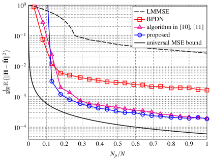
Figure 1: MSE as a function of $N_{p}/N$ ($M=N=M_{p}=100,$ $\text{SNR}=10\text{ dB}$, $L=3$).

For comparison purposes, the performance of the standard basis pursuit denoising (BPDN) algorithm [17], straightforwardly modified to serve as channel estimator for this setting, is also shown. This algorithm assumes that delays and AoAs take values over an equisampled grid of their original domains and always assumes $\|\mathbf{Z}\|=\sqrt{N_{p}M_{p}\sigma^{2}}$, which holds approximately by the law of large numbers. For this example, $256$ samples where considered for both domains discretization, as larger values resulted in high computational complexity with minimal performance improvement. It can be seen that performance of BPDN is significantly worse than the proposed algorithm performance except in the regime of very small $N_{p}$ (but of high MSE as well). Also shown is the performance of the conventional LMMSE estimator obtained by a straightforward generalization of the approach in [26]. It can be seen that LMMSE performs poorly since the second order channel statistics fail to capture the sparsity of the channel, resulting in a minimum of $25\%$ pilot overhead to even achieve an MSE equal to the noise level.

The performance of the decoupled ANM estimator of [10, 11] is also shown in Fig. 1, operating by treating $\mathbf{Y}$ as noiseless, extracting the (decoupled) AoA and delay estimates as the $L$ largest harmonics, and obtaining a denoised channel matrix estimate after coupling the AoA and delay estimates using a procedure similar to the one in [18]. As this algorithm demonstrated large sensitivity to path separability, resulting in extremely poor estimates for channel realizations with very closely spaced paths on the AoA-delay plane, its performance is shown by averaging only over channel realizations satisfying (5) with $d=1/N$. It can be seen that, even under this performance favorable path separation assumption, the algorithm of [10, 11] still performs worse than the proposed one (which effectively operates with $d=0$), over almost all range of $N_{p}$. Note that the proposed algorithm cannot resolve paths that are very closely spaced due to fundamental estimation limits [15] and inevitably results in inaccurate path parameter estimates. However, even though inaccurate, these estimates correspond to MMV atom sets over the AoA and angle domains that can accurately represent the channel when considered as MMV in these domains. This, in addition to the independent treatment of the domains that requires no coupling of parameter estimates, results in a robust algorithm performance even under channel realizations with non-resolvable paths.

Figure 2 shows the MSE of the proposed algorithm and BPDN as a function of $L$ with full observations, i.e., $N_{p}=N$, $M_{p}=M$ (results are similar or $N_{p}<N$ and/or $M_{p}<M$). It can be seen that the proposed algorithm outperforms BPDN for $L$ up to $18$, making it preferable for operations under sparse channels. The MSE bound of (12) is also shown (for $L\geq 2)$, where it can be seen that it serves as a very tight approximation of the actual performance. Note that the performance of the proposed algorithm scales as $L^{2}$, as predicted by (12), which eventually leads to the poorer performance compared to BPDN for large $L$. However, for small $L$, performance is close to the universal MSE bound of (10).

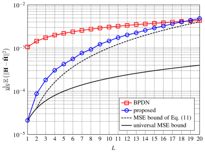
Figure 2: MSE as a function of $L$ ($M=N=N_{p}=M_{p}=100,$ $\text{SNR}=10\text{ dB}$).

VI Conclusions

A low-complexity sequential MMV ANM channel estimation algorithm was proposed for wideband massive MIMO and its performance was analytically characterized in terms of tight MSE bounds. It was demonstrated that the algorithm can provide excellent performance in the regime of low-to-moderate numbers of channel paths, without any restriction on their separability in the AoA-delay plane.

Appendix A Proof of Theorem 1

For simplicity of exposition, the real-valued one-dimensional observation model $\mathbf{y}=\mathbf{S}_{\mathcal{M}_{p}}\mathbf{h}+\mathbf{z}$ is considered first, where $\mathbf{h}=\mathbf{h}(\bm{\phi})\in\mathbb{R}^{M}$ is the vector to be estimated that depends continuously (but, otherwise, arbitrarily), on a parameter vector $\bm{\phi}\in\mathbb{R}^{L}$, $\mathbf{z}\in\mathbb{R}^{M_{p}}$ is a noise vector of i.i.d. Gaussian elements of zero mean and variance $\sigma^{2}/2$, and and $\mathbf{S}_{\mathcal{M}_{p}}$ as defined in (2) with $\mathcal{M}_{p}$ a randomly and uniformly selected subset of $[M]$ with $M_{p}$ elements. For a fixed $\mathcal{M}_{p}$, the covariance matrix of the error $\hat{\mathbf{h}}-\mathbf{h}$ for any estimate $\hat{\mathbf{h}}$ is lower bounded as [14]

$$\mathbb{E}\left(\left(\hat{\mathbf{h}}-\mathbf{h}\right)\left(\hat{\mathbf{h}}-\mathbf{h}\right)^{H}\right)\succeq\nabla_{\bm{\phi}}\left(\mathbf{h}\right)\mathbf{I}^{-1}(\bm{\phi})\nabla_{\bm{\phi}}^{T}\left(\mathbf{h}\right),$$

where the expectation is over noise statistics, $\nabla_{\bm{\phi}}\left(\mathbf{h}\right)\in\mathbb{R}^{M\times L}$ is the gradient of $\mathbf{h}$ w.r.t. to $\bm{\phi}$, and $\mathbf{I}(\bm{\theta})\in\mathbb{R}^{L\times L}$ is the Fisher information matrix for the parameter vector $\bm{\phi}$. The latter is equal to [14]

$$\mathbf{I}(\bm{\theta}) =\frac{2}{\sigma^{2}}\nabla_{\bm{\phi}}^{T}(\mathbb{E}(\mathbf{y}))\nabla_{\bm{\phi}}(\mathbb{E}(\mathbf{y}))$$

$$=\frac{2}{\sigma^{2}}\nabla_{\bm{\phi}}^{T}(\mathbf{S}_{\mathcal{M}_{p}}\mathbf{h})\nabla_{\bm{\phi}}(\mathbf{S}_{\mathcal{M}_{p}}\mathbf{h})$$

$$=\frac{2}{\sigma^{2}}\nabla_{\bm{\phi}}^{T}(\mathbf{h})\mathbf{D}_{\mathcal{M}_{p}}\nabla_{\bm{\phi}}(\mathbf{h}),$$

where $\mathbf{D}_{\mathcal{M}_{p}}\triangleq\mathbf{S}_{\mathcal{M}_{p}}^{T}\mathbf{S}_{\mathcal{M}_{p}}\in\mathbb{R}^{M\times M}$ is a diagonal matrix whose diagonal elements equal $[\mathbf{D}_{\mathcal{M}_{p}}]_{k,k}=1$, if $k\in\mathcal{M}_{p}$, and $0$, if $k\in[M]\setminus\mathcal{M}_{p}$. It follows that the per-element MSE is bounded as

$$\frac{1}{M}\mathbb{E}(\|\hat{\mathbf{h}}-\mathbf{h}\|^{2})$$ (13)

$$= \frac{1}{M}\text{tr}\left\{\mathbb{E}\left(\left(\hat{\mathbf{h}}-\mathbf{h}\right)\left(\hat{\mathbf{h}}-\mathbf{h}\right)^{H}\right)\right\}$$ (14)

$$\geq \frac{\sigma^{2}}{2M}\text{tr}\left\{\nabla_{\bm{\phi}}(\mathbf{h})\left(\nabla_{\bm{\phi}}^{T}(\mathbf{h})\mathbf{D}_{\mathcal{M}_{p}}\nabla_{\bm{\phi}}(\mathbf{h})\right)^{-1}\nabla_{\bm{\phi}}^{T}(\mathbf{h})\right\}.$$ (15)

A lower bound for the MSE can now be obtained by averaging the right-hand side of (15) with respect to the statistics of $\mathcal{M}_{p}$. This is a non-tractable task in general, therefore, looser lower bounds are pursued next.

First note by a trivial application of the Cauchy-Schawrz inequality that it holds $\sum_{k=0}^{L-1}a_{k}\geq L^{2}\left(\sum_{k=0}^{L-1}\frac{1}{a_{k}}\right)^{-1}$ for any sequence $\{a_{k}\}_{k=0}^{L-1}$ of strictly positive elements. Also note that $\nabla_{\bm{\phi}}\left(\mathbf{h}\right)\left(\nabla_{\bm{\phi}}^{T}(\mathbf{h})\mathbf{D}_{\mathcal{M}_{p}}\nabla_{\bm{\phi}}(\mathbf{h})\right)^{-1}\nabla_{\bm{\phi}}^{T}\left(\mathbf{h}\right)$ is a positive semidefinite matrix of rank $L$ and let $\{\lambda_{k}\}_{k=0}^{L-1}$ denote its positive eigenvalues. Noting that $\{\lambda_{k}\}_{k=0}^{L-1}$ are also the eigenvalues of $\left(\nabla_{\bm{\phi}}^{T}(\mathbf{h})\mathbf{D}_{\mathcal{M}_{p}}\nabla_{\bm{\phi}}(\mathbf{h})\right)^{-1}\nabla_{\bm{\phi}}^{T}\left(\mathbf{h}\right)\nabla_{\bm{\phi}}\left(\mathbf{h}\right)$ [27, Theorem 1.3.22], it follows that

$$\text{tr}\left\{\nabla_{\bm{\phi}}\left(\mathbf{h}\right)\left(\nabla_{\bm{\phi}}^{T}(\mathbf{h})\mathbf{D}_{\mathcal{M}_{p}}\nabla_{\bm{\phi}}(\mathbf{h})\right)^{-1}\nabla_{\bm{\phi}}^{T}\left(\mathbf{h}\right)\right\}$$

$$= \text{tr}\left\{\left(\nabla_{\bm{\phi}}^{T}(\mathbf{h})\mathbf{D}_{\mathcal{M}_{p}}\nabla_{\bm{\phi}}(\mathbf{h})\right)^{-1}\nabla_{\bm{\phi}}^{T}\left(\mathbf{h}\right)\nabla_{\bm{\phi}}\left(\mathbf{h}\right)\right\}$$

$$= \sum_{k=0}^{L-1}\lambda_{k}$$

$$\geq L^{2}\left(\sum_{k=0}^{L-1}\frac{1}{\lambda_{k}}\right)^{-1}$$

$$= L^{2}\left(\text{tr}\left\{\left[\left(\nabla_{\bm{\phi}}^{T}(\mathbf{h})\mathbf{D}_{\mathcal{M}_{p}}\nabla_{\bm{\phi}}(\mathbf{h})\right)^{-1}\nabla_{\bm{\phi}}^{T}\left(\mathbf{h}\right)\nabla_{\bm{\phi}}\left(\mathbf{h}\right)\right]^{-1}\right\}\right)^{-1}$$

$$= L^{2}\left(\text{tr}\left\{\mathbf{D}_{\mathcal{M}_{p}}\nabla_{\bm{\phi}}\left(\mathbf{h}\right)\left(\nabla_{\bm{\phi}}^{T}(\mathbf{h})\nabla(\mathbf{h})\right)^{-1}\nabla_{\bm{\phi}}^{T}\left(\mathbf{h}\right)\right\}\right)^{-1}.$$ (16)

It follows from (15) and (16) that the per-element MSE, averaged over $\mathcal{M}_{p}$, is bounded as

$$\frac{1}{M}\mathbb{E}(\|\hat{\mathbf{h}}-\mathbf{h}\|^{2})$$

$$\geq \frac{L^{2}\sigma^{2}}{2M}\mathbb{E}\left(\text{tr}\left\{\mathbf{D}_{\mathcal{M}_{p}}\nabla_{\bm{\phi}}\left(\mathbf{h}\right)\left(\nabla_{\bm{\phi}}^{T}(\mathbf{h})\nabla(\mathbf{h})\right)^{-1}\nabla_{\bm{\phi}}^{T}\left(\mathbf{h}\right)\right\}\right)^{-1}$$

$$\overset{(a)}{\geq} \frac{L^{2}\sigma^{2}}{2M}\left(\text{tr}\left\{\mathbb{E}\left(\mathbf{D}_{\mathcal{M}_{p}}\right)\nabla_{\bm{\phi}}\left(\mathbf{h}\right)\left(\nabla_{\bm{\phi}}^{T}(\mathbf{h})\nabla(\mathbf{h})\right)^{-1}\nabla_{\bm{\phi}}^{T}\left(\mathbf{h}\right)\right\}\right)^{-1}$$

$$\overset{(b)}{=} \frac{L^{2}\sigma^{2}}{2M}\left(\frac{M_{p}}{M}\text{tr}\left\{\nabla_{\bm{\phi}}\left(\mathbf{h}\right)\left(\nabla_{\bm{\phi}}^{T}(\mathbf{h})\nabla(\mathbf{h})\right)^{-1}\nabla_{\bm{\phi}}^{T}\left(\mathbf{h}\right)\right\}\right)^{-1}$$

$$= \frac{L\sigma^{2}}{2M_{p}}$$

where $(a)$ follows by application of Jenssen’s inequality and $(b)$ follows from $\mathbb{E}\left(\mathbf{D}_{\mathcal{M}_{p}}\right)=\frac{M_{p}}{M}\mathbf{I}$, where $\mathbf{I}$ is the $M\times M$ identity matrix, which holds by construction of $\mathcal{M}_{p}$. A straightforward but tedious extension of this proof to the complex valued observation model of (2), noting that $\mathbf{H}$ depends on $4L$ real-valued parameters ($4$ parameters for each path: AoA, delay, gain modulus and angle) leads to the result.

References

- [1] T. L. Marzetta, “Noncooperative cellular wireless with unlimited numbers of base station antennas,” IEEE Trans. Wireless Commun., vol. 9, no. 11, pp. 3590–3600, Nov. 2010.
- [2] A. M. Sayeed, “Deconstructing multi-antenna channels,” IEEE Trans. Signal Process., vol. 50, no. 10, pp. 2563–2579, Oct. 2002.
- [3] C. R. Berger, Z. Wang, J. Huang, and S. Zhou, “Application of compressive sensing to sparse channel estimation,” IEEE Commun. Mag., vol. 48, no. 11, pp. 164–174, Nov. 2010.
- [4] E. J. Candès and C. Fernandez-Granda. Towards a mathematical theory of super-resolution. Communications on Pure and Applied Mathematics, 67(6):906–956, 2014.
- [5] G. Tang, B. Bhaskar, P. Shah, and B. Recht, “Compressed sensing off the grid,” IEEE Trans. Inf. Theory, vol. 59, no. 11, pp. 7465–7490, Nov 2013.
- [6] P. Zhang, L. Gan, S. Sun, and C. Ling, “Atomic norm denoising-based channel estimation for massive multiuser mimo systems,” in IEEE Intl. Conf. on Communications (ICC), Jun. 2015, pp. 4564–4569.
- [7] Y. Chi and Y. Chen, “Compressive two-dimensional harmonic retrieval via atomic norm minimization,” IEEE Trans. Signal Process., vol. 63, no. 4, pp. 1030–1042, Apr. 2015.
- [8] Z. Yang, L. Xie, and P. Stoica, “Vandermonde decomposition of multilevel Toeplitz matrices with application to multidimensional super-resolution”, IEEE Trans. Inf. Theory, vol. 62, no. 6, pp. 3685–3701, Jun. 2016.
- [9] Y. Wang, P. Xu, and Z. Tian, “Efficient channel estimation for massive MIMO systems via truncated two-dimensional atomic norm minimization,” in IEEE Intl. Conf. on Communications (ICC), May 2017.
- [10] J.-F. Cai, W. Xu, and Y. Yang, “Large scale 2D spectral compressed sensing in continuous domain,” in IEEE Intl. Conf. on Acoustics, Speech and Signal Processing (ICASSP), Mar. 2017.
- [11] Z. Tian, Z. Zhang, and Y. Wang, “Low-complexity optimization for two-dimensional direction-of-arrival estimation via decoupled atomic norm minimization,”in IEEE Intl. Conf. on Acoustics, Speech and Signal Processing (ICASSP), Mar. 2017.
- [12] Z. Chen and C. Yang, “Pilot decontamination in wideband massive MIMO systems by exploiting channel sparsity,” IEEE Trans. Wireless Commun., vol. 15, no. 7, pp. 5087–5100, Jul. 2016.
- [13] S. Haghighatshoar and G. Caire, “Massive mimo channel subspace estimation from low-dimensional projections,” IEEE Trans. Signal Process., vol. 65, no. 2, pp. 303–318, Jan. 2017.
- [14] S. M. Kay, Fundamentals of Statistical Signal Processing, Vol. 1: Estimation Theory. Prentice Hall, 1993.
- [15] P. Stoica and R. Moses, Spectral Analysis of Signals. New Jersey: Prentice Hall, 2005.
- [16] V. Chandrasekaran, B. Recht, P. A. Parrilo, and A. S. Willsky, “The convex geometry of linear inverse problems,” Foundations of Computational Mathematics, vol. 12, no. 6, pp. 805–849, 2012.
- [17] S. Foucart and H. Rauhut, A Mathematical Introduction to Compressive Sensing. Birkhäuser, 2013.
- [18] Y. Hua, “Estimating two-dimensional frequencies by matrix enhancement and matrix pencil,” IEEE Trans. Signal Process., vol. 40, no. 9, pp. 2267–2280, 1992.
- [19] B. N. Bhaskar, G. Tang, and B. Recht, “Atomic norm denoising with applications to line spectral estimation,” IEEE Trans. Signal Process., vol. 61, no. 23, pp. 5987–5999, Dec. 2013.
- [20] Y. Chi, “Joint sparsity recovery for spectral compressed sensing,” in IEEE Intl. Conf. on Acoustics, Speech and Signal Processing (ICASSP), May 2014.
- [21] Z. Yang and L. Xie, “Exact joint sparse frequency recovery via optimization methods,” IEEE Trans. Signal Process., vol. 64, no. 19, pp. 5145–5157, Oct. 2016.
- [22] Z. Yang, J. Li, P. Stoica, and L. Xie, “Sparse methods for direction-of-arrival estimation,” 2016, [Online]. Available: https://arxiv.org/abs/1609.09596
- [23] Y. Li and Y. Chi, “Off-the-grid line spectrum denoising and estimation with multiple measurement vectors,” IEEE Trans. Signal Process., vol. 64, no. 5, pp. 1257–1269, Mar. 2016.
- [24] L. Le Magoarou and S. Paquelet, “Parametric channel estimation for massive MIMO,” in IEEE Statistical Signal Processing Workshop (SSP), 2018.
- [25] S. Ahmadi, LTE-Advanced: A Practical Systems Approach to Understanding the 3GPP LTE Releases 10 and 11 Radio Access Technologies. New York, NY, USA: Academic, 2014.
- [26] O. Edfors, M. Sandell, J. J. van de Beek, S. K. Wilson, and P. O. Borjesson, “OFDM channel estimation by singular value decomposition,” IEEE Trans. Commun., vol. 46, no. 7, pp. 931–939, Jul. 1998.
- [27] R. A. Horn and C. R. Johnson, Matrix analysis. Cambridge university press, 2012.