Microlocal analysis of forced waves

Abstract.

We use radial estimates for pseudodifferential operators to describe long time evolution of solutions to $iu_{t}-Pu=f$ where $P$ is a self-adjoint 0th order pseudodifferential operator satisfying hyperbolic dynamical assumptions and where $f$ is smooth. This is motivated by recent results of Colin de Verdière and Saint-Raymond [CS18] concerning a microlocal model of internal waves in stratified fluids.

1. Introduction

Colin de Verdière and Saint-Raymond [CS18] recently found an interesting connection between modeling of internal waves in stratified fluids and spectral theory of zeroth order pseudodifferential operators on compact manifolds. In other problems of fluid mechanics relevance of such operators has been known for a long time, for instance in the work of Ralston [Ra73]. We refer to [CS18] for pointers to current physics literature on internal waves and for numerical and experimental illustrations.

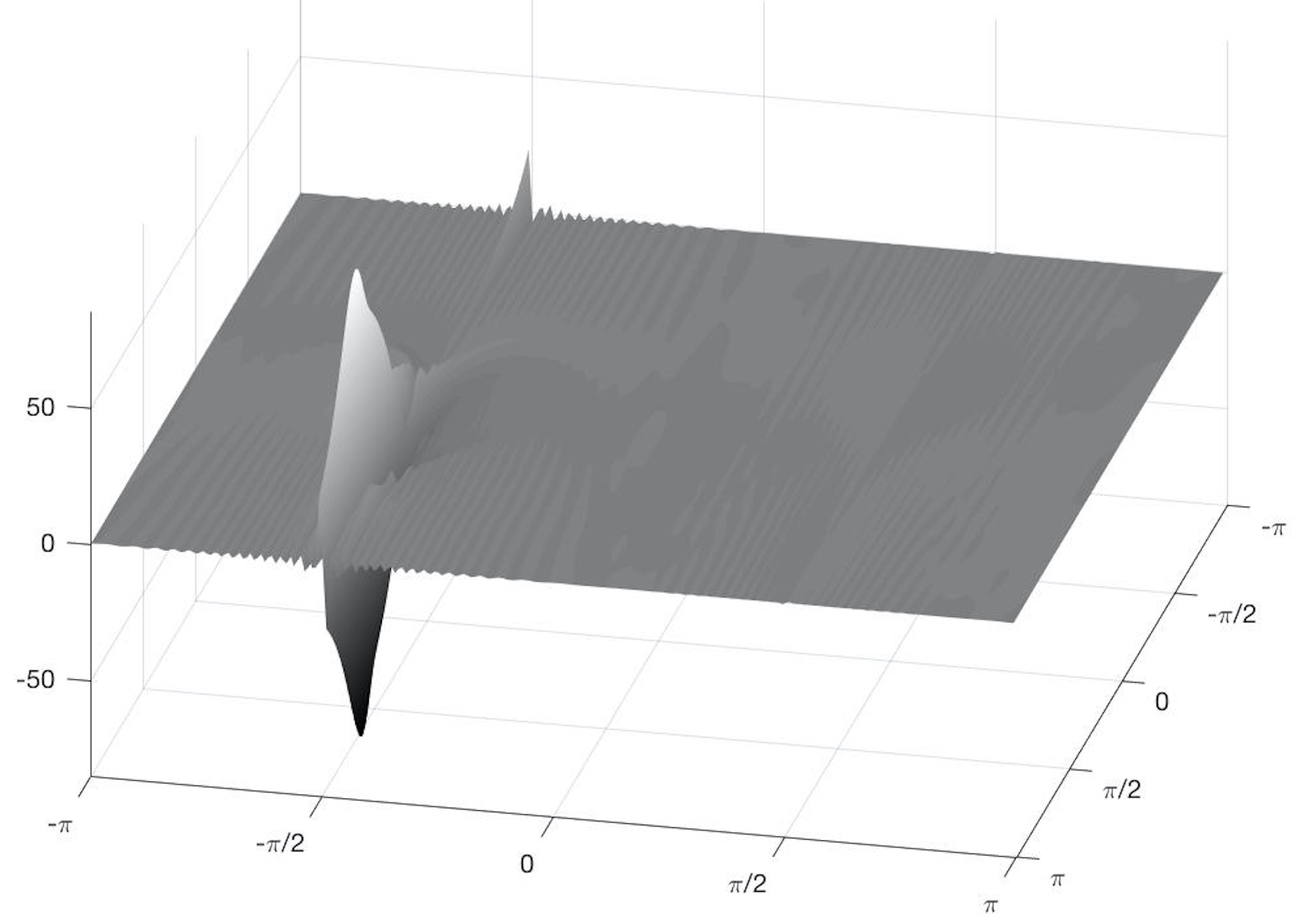
Figure 1. On the left: the plot of the real part of $u(50)$ for $P=\langle D\rangle^{-1}D_{x_{2}}+2\cos x_{1}$ on $\mathbb{T}^{2}$ and $f$ given by a smooth bump function centered at $(-\pi/2,0)$. We see the singularity formation on the line $x_{1}=-\pi/2$. On the right: $\Sigma:=\kappa(p^{-1}(0))\subset\partial\overline{T}^{*}\mathbb{T}^{2}$. The attracting Lagrangian, $\Lambda^{+}_{0}$, comes from the highlighted circles. See §1.3 for a discussion of the examples shown in the figures.

The purpose of this note is to show how the main result of [CS18] (see also [CdV18]) follows from the now standard radial estimates for pseudodifferential operators. In particular, we avoid the use of Mourre theory, normal forms and Fourier integral operators and do not assume that the subprincipal symbols vanish. We also relax some geometric assumptions. The conclusions are formulated in terms of Lagrangian regularity in the sense of Hörmander [HöIII, §25.1]. We illustrate the results with numerical examples. There are many possibilities for refinements but we restrict ourselves to applying off-the-shelf results at this stage.

Radial estimates were introduced by Melrose [Me94] for the study of asymptotically Euclidean scattering and have been developed further in various settings. We only mention some of the more relevant ones: scattering by zeroth order potentials (very close in spirit to the problems considered in [CS18]) by Hassell–Melrose–Vasy [HMV04], asymptotically hyperbolic scattering by Vasy [Va13] (see also [DyZw16, Chapter 5] and [Zw16]) and by Datchev–Dyatlov [DaDy13], in general relativity by Vasy [Va13], Dyatlov [Dy12] and Hintz–Vasy [HiVa16], and in hyperbolic dynamics by Dyatlov–Zworski [DyZw16]. Particularly useful here is the work of Haber–Vasy [HaVa15] which generalized some of the results of [HMV04]. A very general version of radial estimates is presented “textbook style” in [DyZw, §E.4].

1.1. The main result

Motivated by internal waves in linearized fluids the authors of [CS18] considered long time behaviour of solutions to

$$\begin{gathered}(i\partial_{t}-P)u(t)=f,\ \ u(0)=0,\ \ f\in{C^{\infty}}(M),\\ P\in\Psi^{0}(M),\ \ P=P^{*}\end{gathered}$$ (1.1)

where $M$ is a closed surface and $P$ satisfies dynamical assumptions presented in §1.2. By changing $P$ to $P-\omega_{0}$ we can change $f$ to the more physically relevant oscillatory forcing term, $e^{-i\omega_{0}t}f$.

Since the solution $u(t)$ is given by

$$u(t)=-i\int_{0}^{t}e^{-isP}f\,ds=P^{-1}(e^{-itP}-1)f,$$ (1.2)

(where the operator $P^{-1}(e^{-itP}-1)$ is well defined for all $t$ using the spectral theorem), the properties of the spectrum of $P$ play a crucial role in the description of the long time behaviour of $u(t)$. Referring to §1.2 for the precise assumptions we state

Theorem. Suppose that the operator $P$ satisfies assumptions (1.5), (1.8) below and that $0\notin\operatorname{Spec}_{\rm{pp}}(P)$. Then, for any $f\in C^{\infty}(M)$, the solution to (1.1) satisfies

$$\begin{gathered}u(t)=u_{\infty}+b(t)+\epsilon(t),\ \ \|b(t)\|_{L^{2}}\leq C,\ \ \|\epsilon(t)\|_{H^{-\frac{1}{2}-}}\to 0,\ \ t\to\infty,\end{gathered}$$ (1.3)

where (denoting by $H^{-\frac{1}{2}-}$ the intersection of the spaces $H^{-\frac{1}{2}-\varepsilon}$ over $\varepsilon>0$)

$$u_{\infty}\in I^{0}(M;\Lambda^{+}_{0})\subset H^{-\frac{1}{2}-}(M)$$ (1.4)

and $I^{0}(M;\Lambda^{+}_{0})$ is the space of Lagrangian distributions of order $0$ (see §4.1) associated to the attracting Lagrangian $\Lambda^{+}_{0}$ defined in (1.9).

The proof gives other results obtained in [CS18]. In particular, we see that in the neighbourhood of $0$ the spectrum of $P$ is absolutely continuous except for finitely many eigenvalues with smooth eigenfunctions – see §3.2.

In the case of general Morse–Smale flows (allowing for fixed points), Colin de Verdière [CdV18, Theorem 4.3] used a hybrid of Mourre estimates (in particular their finer version given by Jensen–Mourre–Perry [JMP84]) and of the radial estimates [DyZw, §E.4] to obtain a version of (1.3) with an estimate on $\operatorname{WF}(u_{\infty})$. At this stage the purely microlocal approach of this paper would only give $\|\epsilon(t)\|_{H^{-\frac{3}{2}-}}\to 0$.

1.2. Assumptions on $P$

We assume that $M$ is a compact surface without boundary and $P\in\Psi^{0}(M)$ is a 0th order pseudodifferential operator with principal symbol $p\in S^{0}(T^{*}M\setminus 0;\mathbb{R})$ which is homogeneous (of order 0) and has $0$ as a regular value. We also assume that for some smooth density, $dm(x)$, on $M$, $P$ is self-adjoint:

$$\begin{gathered}P\in\Psi^{0}(M),\ \ P=P^{*}\text{ on $L^{2}(M,dm(x))$},\\ p:=\sigma(P),\ \ p(x,t\xi)=p(x,\xi),\ t>0,\ \ dp|_{p^{-1}(0)}\neq 0.\end{gathered}$$ (1.5)

The homogeneity assumption on $p$ can be removed as the results of [DyZw, §E.4] and [DyZw17] we use do not require it. That would however complicate the statement of the dynamical assumptions.

We use the notation of [DyZw, §E.1.3], denoting by $\overline{T}^{*}M$ the fiber-radially compactified co-tangent bundle. Define the quotient map for the ${\mathbb{R}}^{+}$ action, $(x,\xi)\mapsto(x,t\xi)$, $t>0$,

$$\kappa:\overline{T}^{*}M\setminus 0\longrightarrow\partial\overline{T}^{*}M.$$ (1.6)

Denote by $|\xi|$ the norm of a covector $\xi\in T_{x}^{*}M$ with respect to some fixed Riemannian metric on $M$. The rescaled Hamiltonian vector field $|\xi|H_{p}$ commutes with the $\mathbb{R}^{+}$ action and

$$X:=\kappa_{*}(|\xi|H_{p})\quad\text{is tangent to}\quad\Sigma:=\kappa(p^{-1}(0)).$$ (1.7)

Note that $\Sigma$ is an orientable surface since it is defined by the equation $p=0$ in the orientable 3-manifold $\partial\overline{T}^{*}M$.

We now recall the dynamical assumption made by Colin de Verdière and Saint-Raymond [CS18]:

The flow of $$X \Sigma$$ on is a Morse–Smale flow with no fixed points. (1.8)

For the reader’s convenience we recall the definition of Morse–Smale flows generated by $X$ on a surface $\Sigma$ (see [NiZh99, Definition 5.1.1]):

1. $X$ has a finite number of fixed points all of which are hyperbolic;

2. $X$ has a finite number of hyperbolic limit cycles;

3. there are no separatrix connections between saddle fixed points;

4. every trajectory different from (1) and (2) has unique trajectories (1) or (2) as its $\alpha$, $\omega$-limit sets.

As stressed in [CS18], Morse–Smale flows enjoy stability and genericity properties – see [NiZh99, Theorem 5.1.1]. At this stage, following [CS18], me make the strong assumption that there are no fixed points. By the Poincaré–Hopf Theorem that forces $\Sigma$ to be a union of tori.

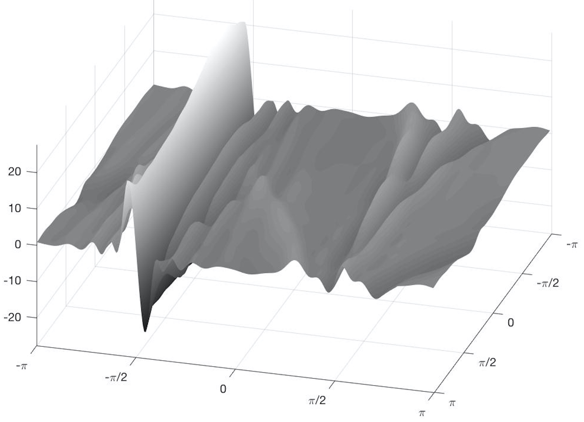
Figure 2. On the left: the plot of the real part of $u(50)$ for $P$ given by (1.11) and $f$ given by a smooth bump function centered at $(-\pi/2,0)$. We see the singularity formation on the line $x_{1}=-\pi/2$ and the slower formation of singularity at $x_{1}=\pi/2$. On the right: $\Sigma:=\kappa(p^{-1}(0))$. The attracting Lagrangian $\Lambda^{+}_{0}$ comes from the highlighted circles.

Under the assumption (1.8), the flow of $X$ on $\Sigma$ has an attractor $L^{+}_{0}$, which is a union of closed attracting curves. We define the following conic Lagrangian submanifold of $T^{*}M\setminus 0$ (see [HöIII, §21.2] and Lemma 2.1):

$$\Lambda^{+}_{0}:=\kappa^{-1}(L^{+}_{0}).$$ (1.9)

1.3. Examples

We illustrate the result with two simple examples on $M:=\mathbb{T}^{2}=\mathbb{S}^{1}\times\mathbb{S}^{1}$ where $\mathbb{S}^{1}=\mathbb{R}/(2\pi\mathbb{Z})$. Denote $D:={1\over i}\partial$. Consider first

$$\begin{gathered}P:=\langle D\rangle^{-1}D_{x_{2}}-2\cos x_{1},\ \ p=|\xi|^{-1}\xi_{2}-2\cos x_{1},\\ |\xi|H_{p}=-{\xi_{1}\xi_{2}\over|\xi|^{2}}\partial_{x_{1}}+{\xi_{1}^{2}\over|\xi|^{2}}\partial_{x_{2}}-2(\sin x_{1})|\xi|\partial_{\xi_{1}},\\ \Lambda^{+}_{0}=\{(\pm\pi/2,x_{2};\xi_{1},0):x_{2}\in\mathbb{S}^{1},\ \pm\xi_{1}<0\}.\end{gathered}$$ (1.10)

In this case $\kappa(p^{-1}(0))$ (with $\kappa$ given in (1.6)) is a union of two tori which do not cover $\mathbb{T}^{2}$ (and thus does not satisfy the assumptions of [CS18] but is covered by the treatment here, and in [CdV18]). See Figure 1 for the plot of $\operatorname{Re}u(t)$, $t=50$ and for a schematic visualization of $\Sigma=\kappa(p^{-1}(0))$.

Our result applies also to the closely related operator

$$\begin{gathered}P:=\langle D\rangle^{-1}D_{x_{2}}-\tfrac{1}{2}\cos x_{1},\quad p=|\xi|^{-1}\xi_{2}-\tfrac{1}{2}\cos x_{1},\\ |\xi|H_{p}=-{\xi_{1}\xi_{2}\over|\xi|^{2}}\partial_{x_{1}}+{\xi_{1}^{2}\over|\xi|^{2}}\partial_{x_{2}}-\tfrac{1}{2}{\sin x_{1}}|\xi|\partial_{\xi_{1}}.\end{gathered}$$ (1.11)

The attracting Lagrangians are the same but the energy surface $\kappa(p^{-1}(0))$ consists of two tori covering $\mathbb{T}^{2}$ (and hence satisfying the assumptions of [CS18]) – see Figure 2.

2. Geometric structure of attracting Lagrangians

In this section we prove geometric properties of the attracting and repulsive Lagrangians for the flow $e^{t|\xi|H_{p}}$ where $p$ satisfies (1.8).

2.1. Sink and source structure

Let $\Sigma(\omega):=\kappa(p^{-1}(\omega))$. If $\delta>0$ is sufficiently small then stability of Morse–Smale flows (and the stability of non-vanishing of $X$) shows that (1.8) is satisfied for $\Sigma(\omega)$, $|\omega|\leq 2\delta$. Let $L^{\pm}_{\omega}\subset\Sigma(\omega)$ be the attractive ($+$) and repulsive ($-$) hyperbolic cycles for the flow of $X$ on $\Sigma(\omega)$. We first establish dynamical properties needed for the application of radial estimates in §3:

Lemma 2.1.

$L^{+}_{\omega}$ is a radial sink and $L^{-}_{\omega}$ a radial source for the Hamiltonian flow of $|\xi|(p-\omega)=|\xi|\sigma(P-\omega)$ in the sense of [DyZw, Definition E.50]. The conic submanifolds

$$\Lambda^{\pm}_{\omega}:=\kappa^{-1}(L^{\pm}_{\omega})\subset T^{*}M\setminus 0$$

are Lagrangian.

Remark. It is not true that $L^{\pm}_{\omega}$ are radial sinks/sources for the Hamiltonian flow of $p-\omega$ since [DyZw, Definition E.50] requires convergence of all nearby Hamiltonian trajectories, not just those on the characteristic set $p^{-1}(\omega)$. See Remark 3 following [DyZw, Definition E.50] for details. The singular behavior of $|\xi|$ at $\xi=0$ is irrelevant here since we are considering a neighbourhood of the fiber infinity.

Proof.

We consider the case of $L^{+}_{\omega}$ as that of $L^{-}_{\omega}$ is similar. To simplify the formulas below we put $\omega:=0$. To see that $\Lambda^{+}_{0}$ is a Lagrangian submanifold we note that $H_{p}$ and $\xi\partial_{\xi}$ are tangent to $\Lambda^{+}_{0}$ and independent (since $X$ does not vanish on $L^{+}_{0}$). Denoting the symplectic form by $\sigma$, we have $\sigma(H_{p},\xi\partial_{\xi})=-dp(\xi\partial_{\xi})=0$, that is $\sigma$ vanishes on the tangent space to $\Lambda^{+}_{0}$.

We next show that $L^{+}_{0}$ is a radial sink. For simplicity assume that it consists of a single attractive closed trajectory of $X$ of period $T>0$, in particular $e^{TX}=I$ on $L^{+}_{0}$. Define the vector field

$$Y:=H_{|\xi|p}$$

which is homogeneous of order 0 on $T^{*}M\setminus 0$ and thus extends smoothly to the fiber-radial compactification $\overline{T}^{*}M\setminus 0$, see [DyZw, Proposition E.5]. We have $Y=X$ on $\partial\overline{T}^{*}M\cap p^{-1}(0)$, thus $L^{+}_{0}\subset\partial\overline{T}^{*}M$ is a closed trajectory of $Y$ of period $T$.

Fix arbitrary $(x_{0},\xi_{0})\in L^{+}_{0}$ and define the linearized Poincaré map $\mathcal{P}$ induced by $de^{TY}(x_{0},\xi_{0})$ on the quotient space $T_{(x_{0},\xi_{0})}(\overline{T}^{*}M)/\mathbb{R}Y_{(x_{0},\xi_{0})}$. The adjoint map $\mathcal{P}^{*}$ acts on covectors in $T^{*}_{(x_{0},\xi_{0})}(\overline{T}^{*}M)$ which annihilate $Y_{(x_{0},\xi_{0})}$. To prove that $L^{+}_{0}$ is a radial sink it suffices to show that the spectral radius of $\mathcal{P}$ is strictly less than 1.

Put $\rho:=|\xi|^{-1}$ which is a boundary defining function on $\overline{T}^{*}M$, then $\Sigma=\partial\overline{T}^{*}M\cap p^{-1}(0)$ is given by $\{p=0,\ \rho=0\}$. Since $Y=X$ on $\Sigma$ and $L^{+}_{0}$ is an attractive cycle for $X$ on $\Sigma$, we have

$$\mathcal{P}|_{\ker(dp)\cap\ker(d\rho)}=c_{1}\quad\text{for some }c_{1}\in\mathbb{R},\ |c_{1}|<1.$$

Since $Y$ is tangent to $\partial\overline{T}^{*}M=\rho^{-1}(0)$, we have $Y\rho=f_{2}\rho$ for some $f_{2}\in C^{\infty}(\overline{T}^{*}M\setminus 0;\mathbb{R})$. Recalling that $Y=H_{|\xi|p}$ we compute $Yp=pH_{|\xi|}p=-pH_{p}(\rho^{-1})=f_{2}p$. Denoting $c_{2}:=f_{2}(x_{0},\xi_{0})$ we then have

$$\mathcal{P}^{*}(dp(x_{0},\xi_{0}))=c_{2}dp(x_{0},\xi_{0}),\quad\mathcal{P}^{*}(d\rho(x_{0},\xi_{0}))=c_{2}d\rho(x_{0},\xi_{0}).$$

Thus $\mathcal{P}$ has eigenvalues $c_{1},c_{2},c_{2}$. On the other hand, $e^{TY}$ preserves the symplectic density $|\sigma\wedge\sigma|$ which has the form $\rho^{-3}d\operatorname{vol}$ for some density $d\operatorname{vol}$ on $\overline{T}^{*}M$ which is smooth up to the boundary. Taking the limit of this statement at $(x_{0},\xi_{0})$ we obtain $\det\mathcal{P}=\det de^{TY}(x_{0},\xi_{0})=c_{2}^{3}$. It follows that $c_{1}=c_{2}$ and thus $\mathcal{P}$ has spectral radius $|c_{1}|<1$ as needed. ∎

For future use we define the conic hypersurfaces in $T^{*}M\setminus 0$

$$\Lambda^{\pm}:=\bigcup_{|\omega|<2\delta}\Lambda^{\pm}_{\omega}.$$ (2.1)

2.2. Geometry of Lagrangian families

We next establish some facts about families of Lagrangian submanifolds which do not need the dynamical assumptions (1.8). Instead we assume that:

• $p:T^{*}M\setminus 0\to\mathbb{R}$ is homogeneous of order 0;

• $\Lambda\subset T^{*}M\setminus 0$ is a conic hypersurface;

• $dp|_{T\Lambda}\neq 0$ everywhere;

• the Hamiltonian vector field $H_{p}$ is tangent to $\Lambda$.

Under these assumptions, the sets

$$\Lambda_{\omega}:=\Lambda\cap p^{-1}(\omega)$$

are two-dimensional conic submanifolds of $T^{*}M\setminus 0$. Moreover, similarly to Lemma 2.1, each $\Lambda_{\omega}$ is Lagrangian. Indeed, if $G$ is a (local) defining function of $\Lambda$, namely $G|_{\Lambda}=0$ and $dG|_{\Lambda}\neq 0$, then $H_{p}$ being tangent to $\Lambda$ implies

$$\{p,G\}=0\quad\text{on}\quad\Lambda.$$ (2.2)

Thus $H_{p},H_{G}$ form a tangent frame on $\Lambda_{\omega}$ and $\sigma(H_{p},H_{G})=0$ on $\Lambda$, where $\sigma$ denotes the symplectic form.

Since $\xi\partial_{\xi}$ is tangent to each $\Lambda_{\omega}$, for any choice of local defining function $G$ of $\Lambda$ we can write

$$\xi\partial_{\xi}=\Phi H_{p}+\Theta H_{G}\quad\text{on}\quad\Lambda$$ (2.3)

for some functions $\Phi,\Theta$ on $\Lambda$. Since the one-dimensional subbundle $\mathbb{R}H_{G}\subset T\Lambda$ is invariantly defined we see that $\Phi\in C^{\infty}(\Lambda;\mathbb{R})$ does not depend on the choice of $G$.

The function $\Phi$ is homogeneous of order 1. Indeed, we can choose $G$ to be homogeneous of order 1 which implies that $[\xi\partial_{\xi},H_{G}]=0$; we also have $[\xi\partial_{\xi},H_{p}]=-H_{p}$. By taking the commutator of both sides of (2.3) with $\xi\partial_{\xi}$ we see that $\xi\partial_{\xi}\Phi=\Phi$. Similarly we see that $\Theta$ is homogeneous of order 0.

On the other hand, taking the commutators of both sides of (2.3) with $H_{p}$ and $H_{G}$ and using the following consequence of (2.2),

$$[H_{p},H_{G}]=H_{\{p,G\}}\in\mathbb{R}H_{G}\quad\text{on}\quad\Lambda,$$

we get the following identities:

$$H_{p}\Phi\equiv 1,\quad H_{G}\Phi\equiv 0\quad\text{on}\quad\Lambda.$$ (2.4)

The function $\Phi$ is related to the $\omega$-derivative of a generating function of $\Lambda_{\omega}$ (see (4.3)):

Lemma 2.2.

Assume that $\Lambda_{\omega}$ is locally given (in some coordinate system on $M$) by

$$\Lambda_{\omega}=\{(x,\xi)\colon x=\partial_{\xi}F(\omega,\xi),\ \xi\in\Gamma_{0}\},$$ (2.5)

where $\xi\mapsto F(\omega,\xi)$ is a family of homogeneous functions of order 1 and $\Gamma_{0}\subset{\mathbb{R}}^{2}\setminus 0$ is a cone. Then we have

$$\partial_{\omega}F(\omega,\xi)=-\Phi(\partial_{\xi}F(\omega,\xi),\xi).$$ (2.6)

Proof.

Let $G$ be a (local) defining function of $\Lambda$. Taking the $\partial_{\xi}$-component of (2.3) at a point $\zeta:=(\partial_{\xi}F(\omega,\xi),\xi)\in\Lambda$ we have

$$\xi=-\Phi(\zeta)\partial_{x}p(\zeta)-\Theta(\zeta)\partial_{x}G(\zeta).$$ (2.7)

On the other hand, differentiating in $\omega$ the identities

$$p(\partial_{\xi}F(\omega,\xi),\xi)=\omega,\quad G(\partial_{\xi}F(\omega,\xi),\xi)=0$$

we get

$$\langle\partial_{x}p(\zeta),\partial_{\xi}\partial_{\omega}F(\omega,\xi)\rangle=1,\quad\langle\partial_{x}G(\zeta),\partial_{\xi}\partial_{\omega}F(\omega,\xi)\rangle=0.$$ (2.8)

Combining (2.7) and (2.8) we arrive at

$$\langle\xi,\partial_{\xi}\partial_{\omega}F(\omega,\xi)\rangle=-\Phi(\zeta)=-\Phi(\partial_{\xi}F(\omega,\xi),\xi)$$

which implies (2.6) since the function $\xi\mapsto\partial_{\omega}F(\omega,\xi)$ is homogeneous of order 1. ∎

Now we specialize to the Lagrangian families used in this paper. We start with a sign condition on $\Phi$ which will be used in §5:

Lemma 2.3.

Suppose that for $\Lambda=\Lambda^{+}$ or $\Lambda=\Lambda^{-}$, with $\Lambda^{\pm}$ given in (2.1) we define $\Phi^{\pm}$ using (2.3). Then for some constant $c>0$

$$\pm\Phi^{\pm}(x,\xi)\geq c|\xi|\quad\text{on}\quad\Lambda^{\pm}.$$ (2.9)

Proof.

We consider the case of $\Phi^{+}$ as the case of $\Phi^{-}$ is handled by replacing $p$ with $-p$. Recall from Lemma 2.1 that each $L^{+}_{\omega}=\kappa(\Lambda^{+}\cap p^{-1}(\omega))$ is a radial sink for the flow $e^{t|\xi|H_{p}}$. Take $(x,\xi)\in\Lambda^{+}$ with $|\xi|$ large. Then (with $S^{*}M$ denoting the cosphere bundle with respect to any fixed metric on $M$)

$$e^{-tH_{p}}(x,\xi)\in S^{*}M\quad\text{for some}\quad t>0,\quad t\sim|\xi|.$$ (2.10)

Recall from (2.4) that $H_{p}\Phi^{+}=1$ on $\Lambda^{+}$. Thus

$$\Phi^{+}(x,\xi)=\Phi^{+}(e^{-tH_{p}}(x,\xi))+t\geq{c}|\xi|-C.$$

It follows that $\Phi^{+}(x,\xi)\geq c|\xi|$ for large $|\xi|$; since $\Phi^{+}$ is homogeneous of order 1, this inequality then holds on the entire $\Lambda^{+}$. ∎

We next construct adapted global defining functions of $\Lambda^{\pm}$ used in §4.2:

Lemma 2.4.

Let $\Lambda^{\pm}$ be defined in (2.1). Then there exist $G_{\pm}\in C^{\infty}(T^{*}M\setminus 0;\mathbb{R})$ such that:

1. $G_{\pm}$ are homogeneous of order 1;

2. $G_{\pm}|_{\Lambda^{\pm}}=0$ and $dG_{\pm}|_{\Lambda^{\pm}}\neq 0$;

3. $H_{p}G_{\pm}=a_{\pm}G_{\pm}$ in a neighborhood of $\Lambda^{\pm}$, where $a_{\pm}\in C^{\infty}(T^{*}M\setminus 0;\mathbb{R})$ are homogeneous of order $-1$ and $a_{\pm}|_{\Lambda^{\pm}}=0$.

Proof.

We construct $G_{+}$, with $G_{-}$ constructed similarly. Fix some function $\widetilde{G}_{+}$ which satisfies conditions (1) and (2) of the present lemma. It exists since $\Lambda^{+}$ is conic and orientable (each of its connected components is diffeomorphic to $[-\delta,\delta]\times\mathbb{S}^{1}\times\mathbb{R}^{+}$). Let $\Theta_{+}$ be defined in (2.3):

$$\xi\partial_{\xi}=\Phi_{+}H_{p}+\Theta_{+}H_{\widetilde{G}_{+}}\quad\text{on}\quad\Lambda^{+}.$$ (2.11)

Commuting both sides of (2.3) with $\xi\partial_{\xi}$ we see that $\Theta_{+}$ is homogeneous of order 0. Moreover $\Theta_{+}$ does not vanish on $\Lambda^{+}$ since $H_{p}$ is not radial (since the flow of $X$ in (1.7) has no fixed points). Choose $G_{+}$ satisfying conditions (1) and (2) and such that

$$G_{+}=\Theta_{+}\widetilde{G}_{+}\quad\text{near }\Lambda^{+}.$$

Then (2.11) gives

$$\xi\partial_{\xi}=\Phi_{+}H_{p}+H_{G_{+}}\quad\text{on}\quad\Lambda^{+}.$$ (2.12)

We have $H_{p}G_{+}|_{\Lambda^{+}}=0$ (since $H_{p}$ is tangent to $\Lambda^{+}$), therefore $H_{p}G_{+}=a_{+}G_{+}$ near $\Lambda^{+}$ for some function $a_{+}$. Commuting both sides of (2.12) with $H_{p}$ and using that $H_{p}\Phi_{+}\equiv 1$ on $\Lambda^{+}$ from (2.4) we have

$$H_{p}=[H_{p},\xi\partial_{\xi}]=H_{p}+[H_{p},H_{G_{+}}]=H_{p}+H_{\{p,G_{+}\}}=H_{p}+a_{+}H_{G_{+}}\quad\text{on}\quad\Lambda^{+}.$$

Since $H_{G_{+}}$ does not vanish on $\Lambda^{+}$, this gives $a_{+}|_{\Lambda^{+}}=0$ as needed. ∎

One application of Lemma 2.4 is the existence of an $H_{p}$-invariant density on $\Lambda^{\pm}$:

Lemma 2.5.

There exist densities $\nu^{\pm}_{\omega}$ on $\Lambda^{\pm}_{\omega}$, $\omega\in[-\delta,\delta]$, such that:

• $\nu^{\pm}_{\omega}$ are homogeneous of order 1, that is $\mathcal{L}_{\xi\partial_{\xi}}\nu^{\pm}_{\omega}=\nu^{\pm}_{\omega}$;

• $\nu^{\pm}_{\omega}$ are invariant under $H_{p}$, that is $\mathcal{L}_{H_{p}}\nu^{\pm}_{\omega}=0$.

Proof.

In the notation of Lemma 2.4 define $\nu^{\pm}_{\omega}$ by $|\sigma\wedge\sigma|=|dp\wedge dG_{\pm}|\times\nu^{\pm}_{\omega}$ where $\sigma$ is the symplectic form. The properties of $\nu^{\pm}_{\omega}$ follow from the identities

$$\mathcal{L}_{\xi\partial_{\xi}}\sigma=\sigma,\quad\mathcal{L}_{\xi\partial_{\xi}}dp=0,\quad\mathcal{L}_{\xi\partial_{\xi}}dG_{\pm}=dG_{\pm},\quad\mathcal{L}_{H_{p}}\sigma=0$$

and the following statement which holds on $\Lambda^{\pm}$:

$$\hskip 115.63243pt\mathcal{L}_{H_{p}}(dp\wedge dG_{\pm})=dp\wedge d(a_{\pm}G_{\pm})=0.\hskip 115.63243pt\qed$$

3. Resolvent estimates

Here we recall the radial estimates as presented in [DyZw, §E.4] specializing to the setting of §1.2. We use the notation of [DyZw, Appendix E] and we write $\|u\|_{s}:=\|u\|_{H^{s}(M)}$.

Since we are not in the semiclassical setting of [DyZw, §E.4] we will only use the usual notion of the wave front set: for $u\in\mathscr{D}^{\prime}(M)$, $\operatorname{WF}(u)\subset T^{*}M\setminus 0$ – see [DyZw, Exercise E.16]. Similarly, for $A\in\Psi^{k}(M)$ we denote by $\operatorname{ell}(A)\subset T^{*}M\setminus 0$ its (nonsemiclassical) elliptic set. Both sets are conic.

3.1. Radial estimates uniformly up to the real axis

Since $L^{-}_{\omega}$ is a radial source we can apply [DyZw, Theorem E.52] (with $h:=1$) to the operator

$$\widetilde{P}_{\epsilon}:=\widetilde{P}-i\epsilon\langle D\rangle\in\Psi^{1}(M),\quad\widetilde{P}:=\langle D\rangle^{1/2}(P-\omega)\langle D\rangle^{1/2},\quad{0\leq\epsilon\ll 1}.$$

Here, since $\widetilde{P}$ is self-adjoint, the threshold regularity condition [DyZw, (E.4.39)] is satisfied for $\widetilde{P}$ with any $s>0$. Strictly speaking one has to modify the proof of [DyZw, Theorem E.52] to include the antiselfadjoint part $-i\epsilon\langle D\rangle$ which has a favorable sign but is of the same differential order as $\widetilde{P}$. (In [DyZw] it was assumed that the principal symbol of $P$ is real-valued near $L^{-}_{\omega}$.) More precisely, we put $\mathbf{P}:=\widetilde{P}$ and $f:=\widetilde{P}_{\epsilon}u$ (instead of $f:=\widetilde{P}u$) in [DyZw, Theorem E.52]. Since $\widetilde{P}_{\epsilon}$ satisfies the sign condition for propagation of singularities [DyZw, Theorem E.47], it suffices to check that the positive commutator estimate [DyZw, Lemma E.49] holds. For that we write

$$\operatorname{Im}\langle f,G^{*}Gu\rangle_{L^{2}}=\operatorname{Im}\langle\widetilde{P}u,G^{*}Gu\rangle_{L^{2}}-\epsilon\operatorname{Re}\big{\langle}\langle D\rangle u,G^{*}Gu\big{\rangle}_{L^{2}}.$$ (3.1)

Here $G\in\Psi^{s}(M)$ is the quantization of an escape function used in the proof of [DyZw, Lemma E.49]; recall that we put $h:=1$. We now estimate the additional term in (3.1):

$$-\operatorname{Re}\big{\langle}\langle D\rangle u,G^{*}Gu\big{\rangle}_{L^{2}} =-\|\langle D\rangle^{1/2}Gu\|_{L^{2}}^{2}+\langle\operatorname{Re}(G^{*}[\langle D\rangle,G])u,u\rangle_{L^{2}}$$

$$\leq C\|B_{1}u\|_{s-1/2}^{2}+C\|u\|_{H^{-N}}^{2}$$

where $B_{1}$ satisfies the properties in the statement of [DyZw, Lemma E.49] and in the last line we used that $G^{*}[\langle D\rangle,G]\in\Psi^{2s}(M)$ has purely imaginary principal symbol and thus $\operatorname{Re}(G^{*}[\langle D\rangle,G])\in\Psi^{2s-1}(M)$. The rest of the proof of [DyZw, Lemma E.49] applies without changes. See also [DyGu16, Lemma 3.7].

Applying the radial estimate in [DyZw, Theorem E.52] for the operator $\widetilde{P}_{\epsilon}=\langle D\rangle^{1/2}(P-\omega-i\epsilon)\langle D\rangle^{1/2}$ to $\langle D\rangle^{-1/2}u$ we see that for every $\widetilde{B}_{-}\in\Psi^{0}(M)$, $\Lambda^{-}\subset\operatorname{ell}(\widetilde{B}_{-})$ there exists $A_{-}\in\Psi^{0}(M)$, $\Lambda^{-}\subset\operatorname{ell}(A_{-})$, such that

$$\begin{gathered}\|A_{-}u\|_{s}\leq C\|\widetilde{B}_{-}(P-\omega-i\epsilon)u\|_{s+1}+C\|u\|_{-N},\\ u\in C^{\infty}(M),\quad s>-\tfrac{1}{2},\quad|\omega|\leq\delta,\quad\epsilon\geq 0,\end{gathered}$$ (3.2)

where $C$ does not depend on $\epsilon,\omega$ and $N$ can be chosen arbitrarily large. The supports of $A_{-}$, $\widetilde{B}_{-}$ are shown on Figure 3.

The inequality (3.2) can be extended to a larger class of distributions (as opposed to $u\in C^{\infty}(M)$): it suffices that $\widetilde{B}_{-}(P-\omega-i\epsilon)u\in H^{s+1}(M)$ and that $A_{-}u\in H^{s^{\prime}}(M)$ for some $s^{\prime}>-\frac{1}{2}$. See Remark 5 after [DyZw, Theorem E.52] or [DyZw16, Proposition 2.6], [Va13, Proposition 2.3].

Figure 3. An illustration of the supports of the operators appearing in (3.2) (left: radial sources) and (3.3) (right: radial sinks). The horizontal line on the top denotes $\partial\overline{T}^{*}M$, the arrows denote flow lines of $|\xi|H_{p}$.

Similarly we have estimates near radial sinks [DyZw, Theorem E.54] for $L^{+}_{\omega}$. Namely, for every $\widetilde{B}_{+}\in\Psi^{0}(M)$, $\Lambda^{+}\subset\operatorname{ell}(\widetilde{B}_{+})$, there exist $A_{+},B_{+}\in\Psi^{0}(M)$, such that $\Lambda^{+}\subset{\rm{ell}}(A_{+})$, $\operatorname{WF}(B_{+})\cap\Lambda^{+}=\emptyset$, and

$$\begin{gathered}\|A_{+}u\|_{s}\leq C\|\widetilde{B}_{+}(P-\omega-i\epsilon)u\|_{s+1}+C\|B_{+}u\|_{s}+C\|u\|_{-N},\\ u\in C^{\infty}(M),\quad s<-\tfrac{1}{2},\quad|\omega|\leq\delta,\quad\epsilon\geq 0,\end{gathered}$$ (3.3)

where $C$ does not depend on $\epsilon,\omega$ and $N$ can be chosen arbitrarily large. The inequality is also valid for distributions $u$ such that $\widetilde{B}_{+}(P-\omega-i\epsilon)u\in H^{s+1}(M)$ and $B_{+}u\in H^{s}(M)$ and it then provides (unconditionally) $A_{+}u\in H^{s}(M)$ – see Remark 2 after [DyZw, Theorem E.54] or [DyZw16, Proposition 2.7], [Va13, Proposition 2.4].

Away from radial points we have the now standard propagation results of Duistermaat–Hörmander [DyZw, Theorem E.47]: if $A,B,\widetilde{B}\in\Psi^{0}(M)$ and for each $(x,\xi)\in\operatorname{WF}(A)$ there exists $T\geq 0$ such that

$$e^{-T|\xi|H_{p}}(x,\xi)\in\operatorname{ell}(B),\ \ e^{-t|\xi|H_{p}}(x,\xi)\in\operatorname{ell}(\widetilde{B}),\ 0\leq t\leq T,$$

then

$$\begin{gathered}\|Au\|_{s}\leq C\|\widetilde{B}(P-\omega-i\epsilon)u\|_{s+1}+C\|Bu\|_{s}+C\|u\|_{-N},\\ u\in C^{\infty}(M),\quad s\in{\mathbb{R}},\quad|\omega|\leq\delta,\quad\epsilon\geq 0,\end{gathered}$$ (3.4)

with $C$ independent of $\epsilon,\omega$. We also have the elliptic estimate [DyZw, Theorem E.33]: (3.4) holds with $B=0$ if $\operatorname{WF}(A)\cap p^{-1}([-\delta,\delta])=\emptyset$ and $\operatorname{WF}(A)\subset\operatorname{ell}(\widetilde{B})$.

Let us now consider

$$u_{\epsilon}=u_{\epsilon}(\omega):=(P-\omega-i\epsilon)^{-1}f,\ \ f\in C^{\infty}(M),\quad|\omega|\leq\delta,\quad\epsilon>0.$$

For any fixed $\epsilon>0$, $P-\omega-i\epsilon\in\Psi^{0}(M)$ is an elliptic operator (its principal symbol equals $p-\omega-i\epsilon$ and $p$ is real-valued), thus by elliptic regularity $u_{\epsilon}\in C^{\infty}(M)$. Combining (3.2), (3.3) and (3.4) we see that for any $\beta>0$

$$\|u_{\epsilon}\|_{-\frac{1}{2}-\beta}\leq C\|f\|_{\frac{1}{2}+\beta}+C\|u_{\epsilon}\|_{-N},$$ (3.5)

and that

$$\|Au_{\epsilon}\|_{s}\leq C\|f\|_{s+1}+C\|u_{\epsilon}\|_{-N},\ \ \operatorname{WF}(A)\cap\Lambda^{+}=\emptyset,\ \ s>-\tfrac{1}{2}.$$ (3.6)

Here the constant $C$ depends on $\beta,s$ but does not depend on $\epsilon,\omega$. Indeed, by our dynamical assumption (1.8) every trajectory $e^{t|\xi|H_{p}}(x,\xi)$ with $(x,\xi)\in p^{-1}([-\delta,\delta])\setminus\Lambda^{+}$ converges to $\Lambda^{-}$ as $t\to-\infty$ (see Figure 4). Applying (3.4) with $B:=A_{-}$ and using (3.2) we get (3.6). Putting $A:=B_{+}$ in (3.6) and using (3.3) we get (3.5).

Figure 4. A schematic representation of the flow $e^{t|\xi|H_{p}}$ on the fiber infinity $\partial\overline{T}^{*}M$ intersected with the energy surface $p^{-1}(\omega)$, with the regularity thresholds for the estimates (3.2) and (3.3).

In particular, we obtain a regularity statement for the limits of the family $(u_{\epsilon})$:

$$\exists\,\epsilon_{j}\to 0,\ u\in\mathscr{D}^{\prime}(M),\ u_{\epsilon_{j}}\xrightarrow{\mathscr{D}^{\prime}(M)}u\quad\Longrightarrow\quad u\in H^{-\frac{1}{2}-}(M),\ \ \operatorname{WF}(u)\subset\Lambda^{+}.$$ (3.7)

Note also that every $u$ in (3.7) solves the equation $(P-\omega)u=f$.

3.2. Regularity of eigenfunctions

Motivated by (3.7) we have the following regularity statement. The proof is an immediate modification of the proof of [DyZw17, Lemma 2.3]: replace $P$ there by $A^{-1}(P-\omega)A^{-1}$ where $A\in\Psi^{-\frac{1}{2}}(M)$ is elliptic, self-adjoint on $L^{2}(M,dm(x))$ (same density with respect to which $P$ is self-adjoint) and invertible. We record this as

Lemma 3.1.

Suppose that $P$ satisfies (1.5) and (1.8). Then for $\omega$ sufficiently small and for $u\in\mathscr{D}^{\prime}(M)$

$$(P-\omega)u\in C^{\infty},\quad\operatorname{WF}(u)\subset\Lambda^{+},\quad\operatorname{Im}\langle(P-\omega)u,u\rangle\geq 0,\quad|\omega|\leq\delta$$

implies that $u\in C^{\infty}(M)$.

In particular this shows that if $(P-\omega)u=0$ and $\operatorname{WF}(u)\subset\Lambda^{+}$ then $u\in L^{2}$, that is $\omega$ lies in the point spectrum $\operatorname{Spec}_{\rm{pp}}(P)$. Radial estimates then show that the number of such $\omega$’s is finite in a neighbourhood of $0$:

Lemma 3.2.

Under the assumptions (1.5) and (1.8), with $\delta$ sufficiently small,

$$\begin{gathered}|\operatorname{Spec}_{\rm{pp}}(P)\cap[-\delta,\delta]|<\infty;\\ (P-\omega)u=0,\ u\in L^{2}(M),\ |\omega|\leq\delta\quad\Longrightarrow\quad u\in C^{\infty}(M).\end{gathered}$$ (3.8)

Proof.

If $u\in L^{2}(M)$ then the threshold assumption in (3.2) is satisfied for $P-\omega$ near $\Lambda^{-}$ and for $-(P-\omega)$ near $\Lambda^{+}$. Using the remark about regularity after (3.2), as well as (3.4) away from sinks and sources, we conclude that

$$\|u\|_{s}\leq C\|u\|_{-N}$$ (3.9)

for any $s$ and $N$. That implies that $u\in C^{\infty}(M)$. Now, suppose that there exists an infinite set of $L^{2}$ eigenfunctions with eigenvalues in $[-\delta,\delta]$:

$$(P-\omega_{j})u_{j}=0,\ \ \ \langle u_{k},u_{j}\rangle_{L^{2}(M)}=\delta_{kj},\ \ \ |\omega_{j}|\leq\delta.$$

Since $u_{j}\rightharpoonup 0$, weakly in $L^{2}$, $u_{j}\to 0$ strongly in $H^{-1}$. But this contradicts (3.9) applied with $s=0$ and $N=1$. ∎

From now on we make the assumption that $P$ has no eigenvalues in $[-\delta,\delta]$:

$$\operatorname{Spec}_{\rm{pp}}(P)\cap[-\delta,\delta]=\emptyset.$$ (3.10)

By Lemma 3.2 we see that (3.10) holds for $\delta$ small enough as long as $0\notin\operatorname{Spec}_{\rm{pp}}(P)$.

3.3. Limiting absorption principle

Using results of §§3.1,3.2 we obtain a version of the limiting absorption principle sufficient for proving (1.3). Radial estimates can also easily give existence of $(P-\omega-i0)^{-1}:H^{\frac{1}{2}+}(M)\to H^{-\frac{1}{2}-}(M)$ but we restrict ourselves to the simpler version and follow Melrose [Me94, §14]. The only modification lies in replacing scattering asymptotics by the regularity result given in Lemma 3.1.

Lemma 3.3.

Suppose that $P$ satisfies (1.5), (1.8), and (3.10). Then for $|\omega|\leq\delta$ and $f\in C^{\infty}(M)$, the limit

$$(P-\omega-i\epsilon)^{-1}f\xrightarrow{H^{-\frac{1}{2}-}(M)}(P-\omega-i0)^{-1}f,\quad\epsilon\to 0+$$

exists. This limit is the unique solution to the equation

$$(P-\omega)u=f,\quad\operatorname{WF}(u)\subset\Lambda^{+},$$ (3.11)

and the map $\omega\mapsto(P-\omega-i0)^{-1}f\in H^{-\frac{1}{2}-}(M)$ is continuous in $\omega\in[-\delta,\delta]$.

Remark. Replacing $P$ with $-P$ we see that there is also a limit

$$(P-\omega+i\epsilon)^{-1}f\xrightarrow{H^{-\frac{1}{2}-}(M)}(P-\omega+i0)^{-1}f,\quad\epsilon\to 0+$$

which satisfies (3.11) with $\Lambda^{+}$ replaced by $\Lambda^{-}$.

Proof.

We first note that Lemma 3.1 and the spectral assumption (3.10) imply that (3.11) has no more than one solution. By (3.7), if a (distributional) limit $(P-\omega-i\epsilon_{j})^{-1}f$, $\epsilon_{j}\to 0$, exists then it solves (3.11).

To show that the limit exists put $u_{\epsilon}:=(P-\omega-i\epsilon)^{-1}f$ and suppose first that $\|u_{\epsilon}\|_{-\frac{1}{2}-\alpha}$ is not bounded as $\epsilon\to 0+$ for some $\alpha>0$. Hence there exists $\epsilon_{j}\to 0+$ such that $\|u_{\epsilon_{j}}\|_{-\frac{1}{2}-\alpha}\to\infty$. Putting $v_{j}:=u_{\epsilon_{j}}/\|u_{\epsilon_{j}}\|_{-\frac{1}{2}-\alpha}$ we obtain

$$(P-\omega-i\epsilon_{j})v_{j}=f_{j},\ \ \|v_{j}\|_{{-\frac{1}{2}-\alpha}}=1,\ \ f_{j}\xrightarrow{C^{\infty}(M)}0.$$ (3.12)

Applying (3.5) with $N=\frac{1}{2}+\alpha$ we see that $v_{j}$ is bounded in $H^{-\frac{1}{2}-\beta}(M)$ for any $\beta>0$. Since $H^{-\frac{1}{2}-\beta}(M)\hookrightarrow H^{-\frac{1}{2}-\alpha}(M)$, $\beta<\alpha$ is compact we can assume, by passing to a subsequence, that $v_{j}\to v$ in $H^{-\frac{1}{2}-\alpha}(M)$. Then $(P-\omega)v=0$ and the same reasoning that led to (3.7) shows that $\operatorname{WF}(v)\subset\Lambda^{+}$. Thus $v$ solves (3.11) with $f\equiv 0$, implying that $v\equiv 0$. This gives a contradiction with the normalization $\|v_{j}\|_{-\frac{1}{2}-\alpha}=1$.

We conclude that $u_{\epsilon}$ is bounded in $H^{-\frac{1}{2}-\alpha}(M)$ for all $\alpha>0$. But then similarly to the previous paragraph $(u_{\epsilon})_{\epsilon\to 0}$ is precompact in $H^{-\frac{1}{2}-\alpha}(M)$ for all $\alpha>0$. Since every limit point has to be the (unique) solution to (3.11), we see that $u_{\epsilon}$ converges as $\epsilon\to 0+$ in $H^{-\frac{1}{2}-\alpha}(M)$ to that solution.

As for continuity in $\omega$, we note that the above proof gives the stronger statement

$$(P-\omega_{j}-i\epsilon_{j})^{-1}f\xrightarrow{H^{-\frac{1}{2}-}(M)}(P-\omega-i0)^{-1}f$$ (3.13)

for all $\epsilon_{j}\to 0+$, $\omega_{j}\to\omega$, and $|\omega_{j}|\leq\delta$. ∎

In §4.2 we will need the following upgraded version of Lemma 3.3:

Lemma 3.4.

Suppose that $P$ satisfies (1.5), (1.8), and (3.10). Let $s<-\frac{1}{2}$ and $g\in H^{s+1}(M)$, $\operatorname{WF}(g)\subset\Lambda^{+}$, where $\Lambda^{+}$ is defined by (2.1). Then for $|\omega|\leq\delta$ the limit

$$(P-\omega-i\epsilon)^{-1}g\xrightarrow{H^{s-}(M)}(P-\omega-i0)^{-1}g,\quad\epsilon\to 0+$$ (3.14)

exists, and $\operatorname{WF}((P-\omega-i0)^{-1}g)\subset\Lambda^{+}$. In particular, for $k\geq 1$ and $f\in C^{\infty}(M)$ the limit

$$(P-\omega-i\epsilon)^{-k}f\xrightarrow{H^{-k+\frac{1}{2}-}(M)}(P-\omega-i0)^{-k}f,\quad\epsilon\to 0+,$$ (3.15)

exists. Finally, $(P-\omega-i0)^{-1}f\in C^{k}_{\omega}([-\delta,\delta];H^{-k-\frac{1}{2}-}(M))$ with $\partial_{\omega}^{k}(P-\omega-i0)^{-1}f=k!(P-\omega-i0)^{-k-1}f$.

Proof.

We follow closely the proof of Lemma 3.3 and put $u_{\epsilon}:=(P-\omega-i\epsilon)^{-1}g$. Since $P-\omega-i\epsilon$ is elliptic for every $\epsilon>0$, we have $u_{\epsilon}\in H^{s+1}(M)$ and $\operatorname{WF}(u_{\epsilon})\subset\operatorname{WF}(g)\subset\Lambda^{+}$, so it remains to establish uniformity as $\epsilon\to 0+$. We use the following version of (3.6) (which follows from the same proof): for every $A\in\Psi^{0}(M)$ with $\operatorname{WF}(A)\cap\Lambda^{+}=\emptyset$ there exists $\widetilde{B}\in\Psi^{0}(M)$ with $\operatorname{WF}(\widetilde{B})\cap\Lambda^{+}=\emptyset$ such that

$$\|Au_{\epsilon}\|_{s^{\prime}}\leq C\|\widetilde{B}g\|_{s^{\prime}+1}+C\|u_{\epsilon}\|_{-N},\quad s^{\prime}>-\textstyle{1\over 2}$$ (3.16)

where the constant $C$ does not depend on $\omega,\epsilon$. We also have the following version of (3.5): there exists $B^{\prime}\in\Psi^{0}(M)$ with $\operatorname{WF}(B^{\prime})\cap\Lambda^{+}=\emptyset$ such that

$$\|u_{\epsilon}\|_{s}\leq C\|g\|_{s+1}+C\|B^{\prime}g\|_{1}+C\|u_{\epsilon}\|_{-N},\quad s<-\textstyle{1\over 2}.$$ (3.17)

Here the norms $\|\widetilde{B}g\|_{s^{\prime}+1}$ and $\|B^{\prime}g\|_{1}$ are finite since $\operatorname{WF}(g)\subset\Lambda^{+}$. From (3.16) and (3.17) we get regularity for limit points of $u_{\epsilon_{j}}$ similarly to (3.7):

$$\exists\,\epsilon_{j}\to 0+,\ u\in\mathscr{D}^{\prime}(M),\ u_{\epsilon_{j}}\xrightarrow{\mathscr{D}^{\prime}(M)}u\quad\Longrightarrow\quad u\in H^{s}(M),\ \ \operatorname{WF}(u)\subset\Lambda^{+}.$$

The existence of the limit (3.14) follows as in the proof of Lemma 3.3, replacing $-{1\over 2}$ by $s$ in Sobolev space orders; here $u=(P-\omega-i0)^{-1}g$ is the unique solution to

$$(P-\omega)u=g,\quad\operatorname{WF}(u)\subset\Lambda^{+}.$$

Iterating this argument, we get existence of the limit (3.15) and continuous dependence of $(P-\omega-i0)^{-k}f\in H^{-k+{1\over 2}-}$ on $\omega\in[-\delta,\delta]$ similarly to (3.13), with $u=(P-\omega-i0)^{-k}f$ being the unique solution to

$$(P-\omega)^{k}u=f,\quad\operatorname{WF}(u)\subset\Lambda^{+}.$$

It remains to show differentiability in $\omega$. For simplicity we assume that $\omega=0$ and show that for $f\in C^{\infty}(M)$,

$$\partial_{\omega}\big{[}(P-\omega-i0)^{-1}f\big{]}\big{|}_{\omega=0}=(P-\omega-i0)^{-2}f\quad\text{in}\quad H^{-\frac{3}{2}-}.$$ (3.18)

The case of higher derivatives is handled by iteration. To show (3.18) we denote $u_{\epsilon}(\omega):=(P-\omega-i\epsilon)^{-1}f$ and write for $\omega\neq 0$, with limits in $H^{-\frac{3}{2}-}$

$${u_{0}(\omega)-u_{0}(0)\over\omega} =\lim_{\epsilon\to 0+}{u_{\epsilon}(\omega)-u_{\epsilon}(0)\over\omega}=\lim_{\epsilon\to 0+}(P-\omega-i\epsilon)^{-1}(P-i\epsilon)^{-1}f$$ (3.19)

$$=(P-\omega-i0)^{-1}(P-i0)^{-1}f.$$

To show the last equality above we first note that the family $(P-\omega-i\epsilon)^{-1}(P-i\epsilon)^{-1}f$ is precompact in $H^{-{3\over 2}-\alpha}(M)$ for any $\alpha>0$ as follows from iterating (3.17). By (3.16) every limit point $u$ of this family as $\epsilon\to 0+$ satisfies $P(P-\omega)u=f$, $\operatorname{WF}(u)\subset\Lambda$ and thus equals $(P-\omega-i0)^{-1}(P-i0)^{-1}f$. Finally, letting $\omega\to 0$ in (3.19) we get (3.18). ∎

4. Lagrangian structure of the resolvent

In this section we describe the Lagrangian structure of the resolvent refining the results of Haber–Vasy [HaVa15] in our special case. To start, we briefly review basic theory of Lagrangian distributions following [HöIV, §25.1].

4.1. Lagrangian distributions

Let $M$ be a compact surface and $\Lambda_{0}\subset T^{*}M\setminus 0$ a conic Lagrangian submanifold without boundary. Denote by $I^{s}(M;\Lambda_{0})\subset\mathcal{D}^{\prime}(M)$ the space of Lagrangian distributions of order $s$ on $M$ associated to $\Lambda_{0}$. They have the following properties:

1. $I^{s}(M;\Lambda_{0})\subset H^{-{1\over 2}-s-}(M)$;

2. for all $u\in I^{s}(M;\Lambda_{0})$ we have $\operatorname{WF}(u)\subset\Lambda_{0}$;

3. if $\Lambda_{1}\subset\Lambda_{0}$ is an open conic subset and $u\in I^{s}(M;\Lambda_{0})$, then $u\in I^{s}(M;\Lambda_{1})$ if and only if $\operatorname{WF}(u)\subset\Lambda_{1}$;

4. for all $A\in\Psi^{k}(M)$ and $u\in I^{s}(M;\Lambda_{0})$ we have $Au\in I^{s+k}(M;\Lambda_{0})$;

5. if additionally $\sigma(A)|_{\Lambda_{0}}=0$, then $Au\in I^{s+k-1}(M;\Lambda_{0})$.

Denote

$$I^{s+}(M;\Lambda_{0}):=\bigcap_{s^{\prime}>s}I^{s^{\prime}}(M;\Lambda_{0}).$$

A simple example on a torus (in the notation of §1.3) is given by

$$u(x):=(x_{1}-\tfrac{\pi}{2}-i0)^{-1}\varphi(x),\ \ \varphi\in C^{\infty}_{\rm{c}}(B(0,1)),\ \ u\in I^{0}(\mathbb{T}^{2};\Lambda_{0}^{+})\subset H^{-\frac{1}{2}-}(\mathbb{T}^{2}),$$ (4.1)

where $\Lambda_{0}^{+}$ is given in (1.10).

To define Lagrangian distributions we use Melrose’s iterative characterization [HöIV, Definition 25.1.1]: $u\in\mathcal{D}^{\prime}(M)$ lies in $I^{s+}(M;\Lambda_{0})$ if and only if $\operatorname{WF}(u)\subset\Lambda_{0}$ and

$$A_{1}\dots A_{\ell}\,u\in H^{-{1\over 2}-s-}(M)\quad\text{for any}\quad A_{1},\dots,A_{\ell}\in\Psi^{1}(M),\ \sigma(A_{j})|_{\Lambda_{0}}=0.$$ (4.2)

Note that [HöIV] uses Besov spaces ${}^{\infty}H^{s}$, however this does not make a difference in (4.2) since $H^{s}\subset{}^{\infty}H^{s}\subset H^{s^{\prime}}$ for all $s^{\prime}<s$, see [HöIII, Proposition B.1.2].

We also need oscillatory integral representations for Lagrangian distributions. Assume that in some local coordinate system on $M$, $\Lambda_{0}$ is given by

$$\Lambda_{0}=\{(x,\xi)\colon x=\partial_{\xi}F(\xi),\ \xi\in\Gamma_{0}\}$$ (4.3)

where $\Gamma_{0}\subset\mathbb{R}^{2}\setminus 0$ is an open cone and $F:\Gamma_{0}\to\mathbb{R}$ is homogeneous of order 1. (Every Lagrangian can be locally written in this form after a change of base, $x$, variables – see [HöIII, Theorem 21.2.16]. Using a pseudodifferential partition of unity we can write every Lagrangian distribution as a sum of expressions of the form (4.4).) Then $u\in I^{s}(M;\Lambda_{0})$ if and only if $u$ can be written (modulo a $C^{\infty}$ function) as

$$u(x)=\int_{\Gamma_{0}}e^{i(\langle x,\xi\rangle-F(\xi))}a(\xi)\,d\xi$$ (4.4)

where $a(\xi)\in C^{\infty}(\mathbb{R}^{2})$ is a symbol of order $s-{1\over 2}$, namely

$$|\partial^{\alpha}_{\xi}a(\xi)|\leq C_{\alpha}\langle\xi\rangle^{s-{1\over 2}-|\alpha|},\quad\xi\in\mathbb{R}^{2}$$ (4.5)

and $a$ is supported in a closed cone contained in $\Gamma_{0}$. See [HöIV, Proposition 25.1.3]. An equivalent way of stating (4.4) is in terms of the Fourier transform $\hat{u}$: $e^{iF(\xi)}\hat{u}(\xi)$ is a symbol, that is, satisfies estimates (4.5).

We finally review properties of the principal symbol of a Lagrangian distribution, used in the proof of Lemma 4.5 below, referring the reader to [HöIV, Chapter 25] for details. The principal symbol of a Lagrangian distribution, $u$, with values in half-densities, $u\in I^{s}(M,\Lambda;\Omega^{\frac{1}{2}}_{M})$, is the equivalence class

$$\sigma(u)\in S^{s+{1\over 2}}(\Lambda;\mathcal{M}_{\Lambda}\otimes\Omega_{\Lambda}^{1\over 2})/S^{s-{1\over 2}}(\Lambda;\mathcal{M}_{\Lambda}\otimes\Omega_{\Lambda}^{1\over 2}),$$

see [HöIV, Theorem 25.1.9], where

• $\Omega_{\Lambda}^{1\over 2}$ is the line bundle of half-densities on $\Lambda$;

• $\mathcal{M}_{\Lambda}$ is the Maslov line bundle; it has a finite number of prescribed local frames with ratios of any two prescribed frames given by a constant of absolute value one. Consequently it has a canonical inner product and does not enter into the calculations below;

• $S^{k}(\Lambda;\mathcal{M}_{\Lambda}\otimes\Omega_{\Lambda}^{1\over 2})$ is the space of sections in $C^{\infty}(\Lambda;\mathcal{M}_{\Lambda}\otimes\Omega_{\Lambda}^{1\over 2})$ which are symbols of order $k$, defined using the dilation operator $(x,\xi)\mapsto(x,\lambda\xi)$, $\lambda>0$, see the discussion on [HöIV, page 13]. In the parametrization (4.4) we have $\sigma(u|dx|^{\frac{1}{2}})=(2\pi)^{-\frac{1}{2}}a(\xi)|d\xi|^{\frac{1}{2}}$. The factor $|d\xi|^{\frac{1}{2}}$ accounts for the difference in the order of the symbol.

If $P\in\Psi^{\ell}(M;\Omega_{M}^{\frac{1}{2}})$ satisfies $\sigma(P)|_{\Lambda}=0$ and $u\in I^{s}(M,\Lambda;\Omega_{M}^{\frac{1}{2}})$ then

$$Pu\in I^{s+\ell-1}(M,\Lambda;\Omega_{M}^{\frac{1}{2}}),\quad\sigma(Pu)=\tfrac{1}{i}L\sigma(u)$$ (4.6)

where $L$ is a first order differential operator on $C^{\infty}(\Lambda;\mathcal{M}_{\Lambda}\otimes\Omega_{\Lambda}^{1\over 2})$ with principal part $H_{p}$. The equation (4.6) is the transport equation for $P$ (the eikonal equation corresponds to $\sigma(P)|_{\Lambda}=0$) – see [HöIV, Theorem 25.2.4]. If $P$ is self-adjoint, then its subprincipal symbol is real-valued by [HöIII, Theorem 18.1.34] and thus by [HöIV, (25.2.12)]

$$L^{*}=-L\quad\text{on }L^{2}(\Lambda;\mathcal{M}_{\Lambda}\otimes\Omega_{\Lambda}^{\frac{1}{2}}).$$ (4.7)

4.2. Lagrangian regularity

We now establish Lagrangian regularity for elements in the range of the operators $(P-\omega\mp i0)^{-1}$ constructed in §3.3:

Lemma 4.1.

Suppose that $P$ satisfies (1.5), (1.8), and (3.10). Let $f\in C^{\infty}(M)$ and

$$u^{\pm}(\omega):=(P-\omega\mp i0)^{-1}f\in H^{-{1\over 2}-}(M),\quad|\omega|\leq\delta.$$

Then $u^{\pm}(\omega)\in I^{0}(M;\Lambda^{\pm}_{\omega})$. Moreover, the symbols of $u^{\pm}(\omega)$ depend smoothly on $\omega$:

$$u^{\pm}(\omega)\in C^{\infty}_{\omega}\big{(}[-\delta,\delta];I^{0}(M;\Lambda^{\pm}_{\omega})\big{)},$$ (4.8)

where the precise meaning of (4.8) is explained in Lemma 4.4 below ((4.25) and Remark 2).

Remark. Lemma 4.1 is similar to the results of Haber and Vasy [HaVa15, Theorem 1.7, Theorem 6.3]. There are two differences: [HaVa15] makes the assumption that the Hamiltonian field $H_{p}$ is radial on $\Lambda^{\pm}_{\omega}$ (which is not true in our case) and it also does not prove smooth dependence of the symbols of $u^{\pm}(\omega)$ on $\omega$. Because of these we give a self-contained proof of Lemma 4.1 below, noting that the argument is simpler in our situation.

We focus on the case of $u^{+}(\omega)$, with regularity of $u^{-}(\omega)$ proved by replacing $P,\,\omega$ with $-P,\,-\omega$, respectively. By Lemma 3.4 we have for every $k\geq 0$

$$u^{+}(\omega)\in C^{k}_{\omega}([-\delta,\delta];H^{-k-{1\over 2}-}(M)),\quad\operatorname{WF}(\partial^{k}_{\omega}u^{+}(\omega))\subset\Lambda^{+}$$ (4.9)

where the wavefront set statement is uniform in $\omega$.

To upgrade (4.9) to Lagrangian regularity, we use the criterion (4.2), applying first order operators $W$ and $D_{\omega}-Q$ to $u^{+}(\omega)$ (see Lemma 4.3 below). Here,

$$W,Q\in\Psi^{1}(M),\quad\sigma(W)=G_{+},\quad\sigma(Q)|_{\Lambda^{+}}=\Phi_{+}$$ (4.10)

where $G_{+}$ is the defining function of $\Lambda^{+}$ constructed in Lemma 2.4 and $\Phi_{+}$ is defined in (2.3). The operator $D_{\omega}-Q$, where $D_{\omega}:={1\over i}\partial_{\omega}$, is used to establish smoothness in $\omega$.

Our proof uses the following corollary of (3.3):

$$\begin{gathered}\text{if}\quad Z\in\Psi^{-1}(M),\quad\sigma(Z)|_{\Lambda^{+}}=0,\quad s<-\textstyle{1\over 2}\quad\text{then}\\ v\in\mathcal{D}^{\prime}(M),\quad\operatorname{WF}(v)\subset\Lambda^{+},\quad(P+Z-\omega)v\in H^{s+1}\quad\Longrightarrow\quad v\in H^{s}.\end{gathered}$$ (4.11)

The addition of $Z$ does not change the validity of (3.3) since it is a subprincipal term whose symbol vanishes on $\Lambda^{+}$, see [DyZw, Theorem E.54].

We also use the following identity valid for any operators $A,B$ on $\mathcal{D}^{\prime}(M)$:

$$B^{m}A=\sum_{j=0}^{m}\binom{m}{j}(\operatorname{ad}^{j}_{B}A)B^{m-j},\ \ \ \ \operatorname{ad}_{B}A:=[B,A],\quad{\operatorname{ad}^{0}_{B}A:=A}.$$ (4.12)

The first step of the proof is to establish regularity with respect to powers of $W$:

Lemma 4.2.

Assume that $v\in\mathcal{D}^{\prime}(M)$ satisfies for some $\ell\geq 0$ and $s<-{1\over 2}$

$$\operatorname{WF}(v)\subset\Lambda^{+},\quad W^{j}(P-\omega)v\in H^{s+1}\quad\text{for}\quad j=0,\dots,\ell.$$ (4.13)

Then $W^{\ell}v\in H^{s}$, where $W$ is defined in (4.10).

Proof.

We argue by induction on $\ell$. For $\ell=0$ the lemma follows immediately from (4.11). We thus assume that $\ell>0$ and the lemma is true for all smaller values of $\ell$, in particular $W^{k}v\in H^{s}$ for $0\leq k\leq\ell-1$. Using (4.12) we write

$$W^{\ell}(P-\omega)=(P-\omega)W^{\ell}+\sum_{j=1}^{\ell}\binom{\ell}{j}(\operatorname{ad}^{j}_{W}P)W^{\ell-j}.$$ (4.14)

We recall from Lemma 2.4 that near $\Lambda^{+}$ we have $H_{G_{+}}p=-a_{+}G_{+}$ where $a_{+}$ is homogeneous of order $-1$ and $a_{+}|_{\Lambda^{+}}=0$. Therefore for $j\geq 1$ we have $H_{G_{+}}^{j}p=-(H_{G_{+}}^{j-1}a_{+})G_{+}$ near $\Lambda^{+}$. Motivated by this we take

$$B_{j}\in\Psi^{-1}(M),\quad\sigma(B_{j})=(-1)^{j-1}i^{j}H_{G_{+}}^{j-1}a_{+},\quad 1\leq j\leq\ell.$$

Then, for $1\leq j\leq\ell$

$$\operatorname{ad}^{j}_{W}P=B_{j}W+R_{j},\quad R_{j}\in\Psi^{-1}\quad\text{microlocally near }\Lambda^{+}.$$ (4.15)

Combining (4.14) and (4.15) we get

$$(P-\omega)W^{\ell}=W^{\ell}(P-\omega)-\sum_{j=1}^{\ell}\binom{\ell}{j}(B_{j}W^{\ell+1-j}+R_{j}W^{\ell-j}).$$ (4.16)

Applying both sides of (4.16) to $v$ and using that $W^{k}v\in H^{s}$ for $0\leq k\leq\ell-1$ and that $W^{\ell}(P-\omega)v\in H^{s+1}$ we get

$$(P+\ell B_{1}-\omega)W^{\ell}v\in H^{s+1}.$$

Since $\sigma(B_{1})=ia_{+}$ vanishes on $\Lambda^{+}$, we apply (4.11) to conclude that $W^{\ell}v\in H^{s}$ as needed. ∎

Since $(P-\omega)u^{+}(\omega)=f\in C^{\infty}(M)$, Lemma 4.2 implies that

$$W^{\ell}u^{+}(\omega)\in H^{-{1\over 2}-}(M)\quad\text{for all}\quad\ell\geq 0.$$ (4.17)

This can be generalized as follows:

$$A_{1}\dots A_{\ell}u^{+}(\omega)\in H^{-{1\over 2}-}(M)\quad\text{for all}\quad A_{1},\dots,A_{\ell}\in\Psi^{1}(M),\ \sigma(A_{j})|_{\Lambda^{+}}=0.$$ (4.18)

To see (4.18), we argue by induction on $\ell$. We have $\sigma(A_{j})=\tilde{a}_{j}G_{+}$ near $\operatorname{WF}(u^{+}(\omega))\subset\Lambda^{+}$ for some $\tilde{a}_{j}$ which is homogeneous of order 0. Taking $\widetilde{A}_{j}\in\Psi^{0}(M)$ with $\sigma(\widetilde{A}_{j})=\tilde{a}_{j}$ we have

$$A_{j}=\widetilde{A}_{j}W+\widetilde{R}_{j}\quad\text{where}\quad\widetilde{R}_{j}\in\Psi^{0}(M)\quad\text{microlocally near}\quad\operatorname{WF}(u^{+}(\omega)).$$

Then we can write $A_{1}\dots A_{\ell}u^{+}(\omega)$ as the sum of two kinds of terms (plus a $C^{\infty}$ remainder):

• the term $\widetilde{A}_{1}\dots\widetilde{A}_{\ell}W^{\ell}u^{+}(\omega)$, which lies in $H^{-{1\over 2}-}(M)$ by (4.17), and

• terms of the form $A^{\prime}_{1}\dots A^{\prime}_{m}u^{+}(\omega)$ where $0\leq m\leq\ell-1$, $A^{\prime}_{j}\in\Psi^{1}(M)$, and $\sigma(A^{\prime}_{j})|_{\Lambda^{+}}=0$, which lie in $H^{-{1\over 2}-}(M)$ by the inductive hypothesis.

From (4.18) we can deduce (similarly to the proof of Lemma 4.4 below) that $u^{+}(\omega)\in I^{0+}(M;\Lambda^{+}_{\omega})$ for each $\omega\in[-\delta,\delta]$. To obtain the smooth dependence of the symbol of $u^{+}(\omega)$ on $\omega$ we generalize (4.17) by additionally applying powers of $D_{\omega}-Q$:

Lemma 4.3.

For all integers $\ell,m\geq 0$ we have

$$W^{\ell}(D_{\omega}-Q)^{m}u^{+}(\omega)\in H^{-{1\over 2}-}(M),\quad|\omega|\leq\delta,$$ (4.19)

and the corresponding norms are bounded uniformly in $\omega$.

Proof.

We argue by induction on $m$, with the case $m=0$ following from (4.17). Put

$$u_{j}(\omega):=(D_{\omega}-Q)^{j}u^{+}(\omega)\in\mathcal{D}^{\prime}(M),\quad 0\leq j\leq m.$$

By (4.9) we have $\operatorname{WF}(u_{j}(\omega))\subset\Lambda^{+}$ for all $j$. Moreover, by the inductive hypothesis

$$W^{\ell}u_{j}(\omega)\in H^{-{1\over 2}-}(M)\quad\text{for all}\quad\ell,\ 0\leq j\leq m-1.$$ (4.20)

Put

$$Y:=[P-\omega,D_{\omega}-Q]=-i-[P,Q]\in\Psi^{0}(M)$$

and note that since $\sigma(Q)|_{\Lambda^{+}}=\Phi_{+}$ and $H_{p}\Phi_{+}\equiv 1$ on $\Lambda^{+}$ by (2.4),

$$\sigma(Y)|_{\Lambda^{+}}=0.$$ (4.21)

Moreover, by (2.4) we have $H_{G_{+}}\Phi_{+}\equiv 0$ on $\Lambda^{+}$, thus the Hamiltonian vector field $H_{\Phi_{+}}$ is tangent to $\Lambda^{+}$. This implies that

$$\sigma(\operatorname{ad}_{Q}^{j}Y)=(-i)^{j}H_{\Phi_{+}}^{j}\sigma(Y)\equiv 0\quad\text{on}\quad\Lambda^{+}\quad\text{for all}\quad j\geq 0.$$ (4.22)

Applying (4.12) with $A:=P-\omega$ and $B:=D_{\omega}-Q$ to $u^{+}(\omega)$ we get

$$(P-\omega)u_{m}(\omega)=(D_{\omega}-Q)^{m}f+\sum_{j=1}^{m}(-1)^{j-1}\binom{m}{j}(\operatorname{ad}_{Q}^{j-1}Y)u_{m-j}(\omega).$$ (4.23)

Since $f\in C^{\infty}$ does not depend on $\omega$, we have $(D_{\omega}-Q)^{m}f\in C^{\infty}$. Next, by the inductive hypothesis (4.20) we have $W^{\ell}u_{m-j}(\omega)\in H^{-{1\over 2}-}$ for all $\ell\geq 0$ and $1\leq j\leq m$. Arguing similarly to (4.18) and using (4.22) we see that $W^{\ell}(\operatorname{ad}_{Q}^{j-1}Y)u_{m-j}(\omega)\in H^{{1\over 2}-}$ as well (here $\operatorname{ad}_{Q}^{j-1}Y\in\Psi^{0}(M)$ which explains the stronger regularity). Thus (4.23) implies

$$W^{\ell}(P-\omega)u_{m}(\omega)\in H^{{1\over 2}-}(M)\quad\text{for all}\quad\ell\geq 0.$$

Now Lemma 4.2 gives $W^{\ell}u_{m}(\omega)\in H^{-{1\over 2}-}$ for all $\ell\geq 0$ as needed.

Finally, uniformity of (4.19) in $\omega$ follows immediately from the proof since the estimates (4.9) and (3.3) that we used are uniform in $\omega$. ∎

We now deduce from Lemma 4.3 that $u^{+}(\omega)$ has microlocal oscillatory integral representations (4.4) with symbols depending smoothly on $\omega$. This shows the weaker version of (4.8) with $I^{0}$ replaced by $I^{0+}$.

Lemma 4.4.

Assume that $\mathcal{U}\subset T^{*}M\setminus 0$ is an open conic set such that $\Lambda^{+}_{\omega}\cap\mathcal{U}$ are given in the form (2.5) in some local coordinate system on $M$:

$$\Lambda^{+}_{\omega}\cap\mathcal{U}=\{(x,\xi)\colon x=\partial_{\xi}F(\omega,\xi),\ \xi\in\Gamma_{0}\},\quad|\omega|\leq\delta$$ (4.24)

where $\xi\mapsto F(\omega,\xi)$ is homogeneous of order 1 and $\Gamma_{0}\subset\mathbb{R}^{2}\setminus 0$ is an open cone. Let $A\in\Psi^{0}(M)$, $\operatorname{WF}(A)\subset\mathcal{U}$. Then,

$$Au^{+}(\omega,x)=\int_{\Gamma_{0}}e^{i(\langle x,\xi\rangle-F(\omega,\xi))}a(\omega,\xi)\,d\xi+C^{\infty}_{\omega,x},\quad|\omega|\leq\delta$$ (4.25)

where $a(\omega,\xi)$ is a smooth in $\omega$ family of symbols of order $-{1\over 2}+$ in $\xi$ supported in a closed cone inside $\Gamma_{0}$, see (4.5).

Remarks. 1. The statement (4.25) means that $u^{+}(\omega)$ can be represented as (4.4), microlocally in every closed cone contained in $\mathcal{U}$.

2. When (4.25) holds for every choice of parametrization (4.24) we write

$$u^{+}(\omega)\in C^{\infty}_{\omega}\big{(}[-\delta,\delta];I^{0+}(M;\Lambda^{+}_{\omega})\big{)},$$

with the analogous notation in the case of $u^{-}(\omega)$. That explains the statement of Lemma 4.1.

Proof.

Since $(P-\omega)u^{+}(\omega)=f\in C^{\infty}(M)$, it follows from Lemma 4.3 that for all $m,\ell,r\geq 0$

$$(D_{\omega}-Q)^{m}W^{\ell}(P-\omega)^{r}u^{+}(\omega)\in H^{-{1\over 2}-}(M)$$

This can be generalized as follows:

$$(D_{\omega}-Q(\omega))^{m}A_{1}(\omega)\dots A_{\ell}(\omega)u^{+}(\omega)\in H^{-{1\over 2}-}(M)$$ (4.26)

for all $m$ and all $A_{1}(\omega),\dots,A_{\ell}(\omega),Q(\omega)\in\Psi^{1}(M)$ depending smoothly on $\omega\in[-\delta,\delta]$ and such that $\sigma(A_{j}(\omega))|_{\Lambda^{+}_{\omega}}=0$, $\sigma(Q(\omega))|_{\Lambda^{+}_{\omega}}=\Phi_{+}$. The proof is similar to the proof of (4.18), using the decomposition

$$\begin{gathered}A_{j}(\omega)=A^{\prime}_{j}(\omega)W+A^{\prime\prime}_{j}(\omega)(P-\omega)+R_{j}(\omega)\\ \text{where}\quad R_{j}(\omega)\in\Psi^{0}\quad\text{microlocally near}\quad\operatorname{WF}(u^{+}(\omega))\end{gathered}$$

for some $A^{\prime}_{j}(\omega),A^{\prime\prime}_{j}(\omega)\in\Psi^{0}(M)$ depending smoothly on $\omega\in[-\delta,\delta]$.

Since $\operatorname{WF}(A\partial^{k}_{\omega}u^{+}(\omega))\subset\Lambda^{+}\cap p^{-1}([-\delta,\delta])\cap\mathcal{U}$ for all $k$, by the Fourier inversion formula we can write $Au^{+}(\omega)$ in the form (4.25) for some $a(\omega,\xi)$ which is smooth in $\omega,\xi$ and supported in $\xi\in\Gamma_{1}$ where $\Gamma_{1}\subset\Gamma_{0}$ is some closed cone. It remains to show the following growth bounds as $\xi\to\infty$: for every $\varepsilon>0$

$$\langle\xi\rangle^{-{1\over 2}+|\alpha|-\varepsilon}\partial^{m}_{\omega}\partial^{\alpha}_{\xi}a(\omega,\xi)\in L^{\infty}_{\omega}([-\delta,\delta];L^{2}_{\xi}(\mathbb{R}^{2})).$$ (4.27)

(From (4.27) one can get $L^{\infty}_{\xi}$ bounds using Sobolev embedding as in the proof of [HöIV, Proposition 25.1.3].)

Denote by $\mathcal{I}(a)$ the integral on the right-hand side of (4.25). By Lemma 2.2 we have $\partial_{\omega}F(\omega,\xi)=-\Phi_{+}(\partial_{\xi}F(\omega,\xi),\xi)$, therefore we may take $Q(\omega):=-\partial_{\omega}F(\omega,D_{x})$ to be a Fourier multiplier. The operators

$$A_{jk}(\omega):=D_{x_{k}}\big{(}(\partial_{\xi_{j}}F)(\omega,D_{x})-x_{j}\big{)},\quad j,k\in\{1,2\},$$

lie in $\Psi^{1}$ and satisfy $\sigma(A_{jk}(\omega))|_{\Lambda^{+}_{\omega}}=0$. We have

$$(D_{\omega}-Q(\omega))\mathcal{I}(a)=\mathcal{I}(D_{\omega}a),\quad A_{jk}(\omega)\mathcal{I}(a)=\mathcal{I}(\xi_{k}D_{\xi_{j}}a).$$

Also, if $\mathcal{I}(a)\in H^{-{1\over 2}-}$ uniformly in $\omega$, then $\langle\xi\rangle^{-{1\over 2}-\varepsilon}a(\omega,\xi)\in L^{\infty}_{\omega}([-\delta,\delta];L^{2}_{\xi}(\mathbb{R}^{2}))$. Applying (4.26) with the operators $D_{\omega}-Q(\omega)$ and $A_{jk}(\omega)$ we get (4.27), finishing the proof. ∎

We finally show the stronger statement of Lemma 4.1 (with $I^{0}$ instead of $I^{0+}$) using the transport equation satisfied by the principal symbol:

Lemma 4.5.

We have

$$u^{+}(\omega)\in C^{\infty}_{\omega}\big{(}[-\delta,\delta];I^{0}(M;\Lambda_{\omega}^{+})\big{)},$$

that is (4.25) holds where $a(\omega,\xi)$ is a symbol of order $-{1\over 2}$ in $\xi$.

Proof.

In our setting $P\in\Psi^{0}(M)$ is self-adjoint with respect to a smooth density on $M$ – see (1.5). Using that density to trivialize the half-density bundle we obtain a self-adjoint operator $P\in\Psi^{0}(M;\Omega^{1\over 2}_{M})$.

Let $a^{+}\in S^{{1\over 2}+}(\Lambda^{+}_{\omega};\mathcal{M}_{\Lambda^{+}_{\omega}}\otimes\Omega_{\Lambda^{+}_{\omega}}^{1\over 2})$ be a representative of $\sigma(u^{+}(\omega))$. Using the transport equation (4.6) and $(P-\omega)u^{+}(\omega)=f\in C^{\infty}(M)$, we have

$$b^{+}:=La^{+}\in S^{-{3\over 2}+}(\Lambda^{+}_{\omega};\mathcal{M}_{\Lambda^{+}_{\omega}}\otimes\Omega_{\Lambda^{+}_{\omega}}^{1\over 2}),$$ (4.28)

where $L$ is a first-order differential operator on $C^{\infty}(\Lambda^{+}_{\omega};\mathcal{M}_{\Lambda^{+}_{\omega}}\otimes\Omega_{\Lambda^{+}_{\omega}}^{1\over 2})$ with principal part given by $H_{p}$ and $L^{*}=-L$ by (4.7).

We trivialize $\Omega^{1\over 2}_{\Lambda^{+}_{\omega}}$ using the density $\nu^{+}_{\omega}$ constructed in Lemma 2.5 and write

$$a^{+}=\tilde{a}^{+}\sqrt{\nu^{+}_{\omega}},\quad b^{+}=\tilde{b}^{+}\sqrt{\nu^{+}_{\omega}}.$$

where $\tilde{a}^{+}\in S^{0+}(\Lambda^{+}_{\omega};\mathcal{M}_{\Lambda^{+}_{\omega}})$, $\tilde{b}^{+}\in S^{-2+}(\Lambda^{+}_{\omega};\mathcal{M}_{\Lambda^{+}_{\omega}})$. By (4.28) we have

$$(H_{p}+V)\tilde{a}^{+}=\tilde{b}^{+}$$ (4.29)

where $H_{p}$ naturally acts on sections of the locally constant bundle $\mathcal{M}_{\Lambda^{+}_{\omega}}$ and $V\in C^{\infty}(\Lambda^{+}_{\omega})$ is homogeneous of order $-1$. Moreover, since $L^{*}=-L$ we have

$$\operatorname{Re}V=\tfrac{1}{2}(\mathcal{L}_{H_{p}}\nu^{+}_{\omega})/\nu^{+}_{\omega}=0$$

using Lemma 2.5.

By (4.29) for all $(x,\xi)\in\Lambda^{+}_{\omega}$ and $t\geq 0$ we have

$$\tilde{a}^{+}(x,\xi)={\big{(}}e^{-t(H_{p}+V)}\tilde{a}^{+}{\big{)}}(x,\xi)+\int_{0}^{t}{\big{(}}e^{-s(H_{p}+V)}\tilde{b}^{+}{\big{)}}(x,\xi)\,ds.$$ (4.30)

Since $\operatorname{Re}V=0$ we have $|e^{-t(H_{p}+V)}\tilde{a}^{+}(x,\xi)|=|\tilde{a}^{+}(e^{-tH_{p}}(x,\xi))|$ and same is true for $\tilde{b}^{+}$.

Take $(x,\xi)\in\Lambda^{+}_{\omega}$ with $|\xi|$ large. As in (2.10) choose $t\geq 0$, $t\sim|\xi|$, such that $e^{-tH_{p}}(x,\xi)\in S^{*}M$; we next apply (4.30). The first term on the right-hand side is bounded uniformly as $\xi\to\infty$. Same is true for the second term since the function under the integral is $\mathcal{O}((t-s)^{-2+})$. It follows that $\tilde{a}^{+}(x,\xi)$ is bounded as $\xi\to\infty$.

Since $[\xi\partial_{\xi},H_{p}+V]=-H_{p}-V$, we have for all $j$

$$(H_{p}+V)(\xi\partial_{\xi})^{j}\tilde{a}^{+}=(\xi\partial_{\xi}+1)^{j}\tilde{b}^{+}\in S^{-2+}(\Lambda^{+}_{\omega};\mathcal{M}_{\Lambda^{+}_{\omega}}).$$ (4.31)

It follows that $(H_{p}+V)^{\ell}(\xi\partial_{\xi})^{j}\tilde{a}^{+}=\mathcal{O}(\langle\xi\rangle^{-\ell})$ for all $j,\ell$: the case $\ell=0$ follows from (4.30) applied to (4.31) and the case $\ell\geq 1$ follows directly from (4.31). Since $\xi\partial_{\xi}$ and $H_{p}$ form a frame on $\Lambda^{+}_{\omega}$, we have $\tilde{a}^{+}\in S^{0}(\Lambda^{+}_{\omega};\mathcal{M}_{\Lambda^{+}_{\omega}})$ which implies that $u^{+}_{\omega}\in I^{0}(M;\Lambda^{+}_{\omega})$. ∎

Remark. It is instructive to consider the transport equation (4.29) in the microlocal model used in [CS18]: near a model sink $\Lambda^{+}_{\omega}=\{(-\omega,x_{2};\xi_{1},0):\xi_{1}>0\}\subset T^{*}({\mathbb{R}}_{x_{1}}\times\mathbb{S}^{1}_{x_{2}})\subset 0$ (see the global examples in §1.3) we consider $p(x,\xi):=\xi_{1}^{-1}\xi_{2}-x_{1}$. We are then solving $(p(x,D)-\omega)u^{+}(\omega)\equiv 0$ microlocally near $\Lambda^{+}_{\omega}$ (see [DyZw, Definition E.29]) and for that we expand the symbol on $u^{+}_{\omega}$ into Fourier modes in $x_{2}$,

$$u^{+}_{\omega}(x)=\frac{1}{2\pi}\int_{\mathbb{R}}\sum_{n\in{\mathbb{Z}}}\hat{a}_{\omega}^{+}(n,\xi_{1})e^{i(x_{1}+\omega)\xi_{1}}e^{inx_{2}}\,d\xi_{1},\ \ a_{\omega}^{+}=\sum_{n\in{\mathbb{Z}}}\hat{a}_{\omega}^{+}(n,\xi_{1})e^{inx_{2}}|d\xi_{1}dx_{2}|^{\frac{1}{2}}.$$

The Fourier coefficients should satisfy $(\xi_{1}^{-1}n+D_{\xi_{1}})\tilde{a}_{\omega}^{+}(n,\xi_{1})=0$ for $\xi_{1}>1$ and $\tilde{a}_{+}^{\omega}(n,\xi_{1})=0$ for $\xi_{1}<-1$. Hence the symbol is given by

$$a_{\omega}^{+}=\tilde{a}^{+}(\omega)|dx_{2}d\xi_{1}|^{1\over 2},\quad\tilde{a}^{+}(x_{2},\xi_{1})=\sum_{n\in{\mathbb{Z}}}\xi_{1}^{-in}a_{n}(\omega)e^{inx_{2}},\quad a_{n}(\omega)=\mathcal{O}(\langle n\rangle^{-\infty}).$$

Hence, the symbol is very “non-classical” in the sense that it does not have an expansion in powers of $\xi_{1}$. In the general case an analogous conclusion follows from the structure of (4.29).

5. An asymptotic result

We now place ourselves in the setting of Lemma 4.1 and assume that $u(\omega)\in C^{\infty}_{\omega}([-\delta,\delta];I^{0}(M;\Lambda_{\omega}))$ in the sense described in Lemma 4.5, where $\Lambda_{\omega}=\Lambda^{+}_{\omega}$ or $\Lambda_{\omega}=\Lambda^{-}_{\omega}$. We are interested in the asymptotic behaviour as $t\to\infty$ of

$$I(t):=\int_{0}^{t}\int_{\mathbb{R}}e^{-is\omega}\varphi(\omega)u(\omega)\,d\omega ds\in\mathcal{D}^{\prime}(M),\ \ \varphi\in C^{\infty}_{\mathrm{c}}((-\delta,\delta)).$$ (5.1)

We have the following local asymptotic result.

Lemma 5.1.

Suppose that $u(\omega)\in\mathcal{D}^{\prime}({\mathbb{R}}^{2})$ is given by

$$\begin{gathered}u(\omega)=u(\omega,x)=\frac{1}{(2\pi)^{2}}\int_{\Gamma_{0}}e^{i(\langle x,\xi\rangle-F(\omega,\xi))}a(\omega,\xi)\,d\xi,\end{gathered}$$ (5.2)

where $\Gamma_{0}$, $F$, and $a$ satisfy the general conditions in (4.25). Suppose also that

$$\varepsilon\partial_{\omega}F(\omega,\xi)<0,\quad\varepsilon=\pm,\quad\xi\in\Gamma_{0},\quad|\omega|\leq\delta.$$ (5.3)

Then as $t\to\infty$,

$$\begin{gathered}I(t)=u_{\infty}+b(t)+v(t),\ \ \|{b}(t)\|_{H^{\frac{1}{2}-}}\leq C,\ \ v(t)\to 0\text{ in $H^{-\frac{1}{2}-}({\mathbb{R}}^{2})$},\\ u_{\infty}=\left\{\begin{array}[]{ll}2\pi\varphi(0)u(0),&\varepsilon=+;\\ \ \ \ \ \ 0,&\varepsilon=-.\end{array}\right.\end{gathered}$$ (5.4)

Proof.

We start by remarking that we can assume that the amplitude $a$ is supported away from $\xi=0$. The remaining contribution can be absorbed into $b(t)$: if $a=a(\omega,\xi)=0$ for $|\xi|>C$ then

$$\begin{split}\widehat{w}(t,\xi)&:=\int_{0}^{t}\int_{\mathbb{R}}e^{-is\omega}e^{-iF(\omega,\xi)}a(\omega,\xi)\varphi(\omega)d\omega ds\\ &=\int_{0}^{t}\int_{\mathbb{R}}\left[(1+s^{2})^{-1}(1+D_{\omega}^{2})e^{-is\omega}\right]e^{-iF(\omega,\xi)}a(\omega,\xi)\varphi(\omega)d\omega ds,\end{split}$$

which by integration by parts in $\omega$ is bounded in $t$ and compactly supported in $\xi$.

Since $u(\omega,x)$ has nice structure on the Fourier transform side it is natural to consider the Fourier transform of $x\mapsto I(t)(x)$, $J(t,\xi):=\mathcal{F}_{x\to\xi}{I(t)}$, where

$$J(t,\xi)=\frac{1}{h}\int_{0}^{ht}\int_{\mathbb{R}}e^{-\frac{i}{h}(F(\omega,\eta)+r\omega)}a(\omega,\eta/h)\varphi(\omega)\,d\omega dr,\quad\xi=\frac{\eta}{h},\ \ \eta\in\mathbb{S}^{1}.$$ (5.5)

From the assumptions on $a$ we have $J(t,\xi)=0$ unless $\eta\in\Gamma_{1}$, where $\Gamma_{1}\subset\Gamma_{0}$ is a closed cone. The phase in $J(t)$ is stationary when

$$\omega=0,\ \ r=r(\eta):=-\partial_{\omega}F(0,\eta).$$ (5.6)

From (5.3), $\partial_{\omega}F(\omega,\eta)\neq 0$ and this means that for some $\gamma>0$,

$$|r+\partial_{\omega}F(\omega,\eta)|>c\langle r\rangle,\ \ \eta\in\mathbb{S}^{1}\cap\Gamma_{1},\ \ |\omega|\leq\delta,\ \ |r|\notin(\gamma,1/\gamma).$$ (5.7)

Let $\chi\in C^{\infty}_{\mathrm{c}}((\gamma/2,2/\gamma);[0,1])$ be equal to $1$ on $(\gamma,1/\gamma)$. Using integration by parts based on

$${h^{N}}\left(-(r+\partial_{\omega}F(\omega,\eta))^{-1}D_{\omega}\right)^{N}e^{-\frac{i}{h}(F(\omega,\eta)+r\omega)}=e^{-\frac{i}{h}(F(\omega,\eta)+r\omega)},$$

and (5.7) we see that, by taking $N\geq 2$,

$$\begin{split}&\frac{1}{h}\int_{0}^{ht}\int_{\mathbb{R}}(1-\chi(r))e^{-\frac{i}{h}(F(\omega,\eta)+r\omega)}a(\omega,\eta/h)\varphi(\omega)\,d\omega dr=\mathcal{O}(h^{N-1}),\end{split}$$

uniformly in $t\geq 0$. Hence, for all $N$

$$\begin{gathered}J(t)=\widetilde{J}(t)+\mathcal{F}_{x\mapsto\xi}u_{0}(t),\ \ \sup_{t\geq 0}\|u_{0}(t)\|_{H^{N}}\leq C_{N},\\ \widetilde{J}(t,\xi):=\frac{1}{h}\int_{0}^{ht}\int_{\mathbb{R}}\chi(r)e^{-\frac{i}{h}(F(\omega,\eta)+r\omega)}a(\omega,\eta/h)\varphi(\omega)\,d\omega dr,\quad\xi=\frac{\eta}{h},\ \eta\in\mathbb{S}^{1}.\end{gathered}$$

When $ht\geq 2/\gamma$, we have $\widetilde{J}(t,\xi)=\widetilde{J}(\infty,\xi)$ due to the support property of $\chi$. In particular this implies that $\widetilde{J}(t,\xi)\to\widetilde{J}(\infty,\xi)$ as $t\to\infty$ pointwise in $\xi$. We apply the standard method of stationary phase to $\widetilde{J}(\infty)$ noting that

$$-\partial^{2}_{\omega,r}(F(\omega,\eta)+r\omega)=\begin{bmatrix}-\partial_{\omega}^{2}F&-1\\ -1&0\end{bmatrix},\ \ \ \operatorname{sgn}\partial^{2}_{\omega,r}(F(\omega,\eta)-r\omega)=0.$$

Therefore

$$\widetilde{J}(\infty,\xi)=\left\{\begin{array}[]{ll}2\pi a(0,\xi)\varphi(0)e^{-iF(0,\xi)}+\mathcal{O}(\langle\xi\rangle^{-\frac{3}{2}+}),&\partial_{\omega}F(0,\xi)<0,\\ \ \ \ \ \ \ \ \ \ \ \ \ \mathcal{O}(\langle\xi\rangle^{-\infty}),&\partial_{\omega}F(0,\xi)>0.\end{array}\right.$$ (5.8)

Hence to obtain (5.4) all we need to show is that $\widetilde{J}(t,\xi)=\mathcal{O}(\langle\xi\rangle^{-\frac{1}{2}+})$ uniformly in $t$ as then by dominated convergence,

$$\begin{split}\langle\xi\rangle^{-\frac{1}{2}-}\widetilde{J}(t)&\xrightarrow{L^{2}({\mathbb{R}}^{2},d\xi)}\langle\xi\rangle^{-\frac{1}{2}-}\widetilde{J}(\infty),\ \ \ t\to+\infty,\end{split}$$

that is,

$$\widetilde{I}(t):=\mathcal{F}^{-1}_{\xi\to x}\widetilde{J}(t)\xrightarrow{H^{-\frac{1}{2}-}({\mathbb{R}}^{2})}\mathcal{F}^{-1}_{\xi\to x}\widetilde{J}_{\infty}(t),\ \ \ t\to+\infty.$$

Here the $\mathcal{O}(\langle\xi\rangle^{-\frac{3}{2}+})$ remainder in (5.8) can be put into $b(t)$ in (5.4).

The uniform boundedness of $\widetilde{J}(t,\xi)$ follows from the following simple lemma:

Lemma 5.2.

Suppose that $A=A(s,\omega)\in C^{\infty}_{\mathrm{c}}({\mathbb{R}}^{2})$ and $G\in{C^{\infty}}({\mathbb{R}};{\mathbb{R}})$. Then as $h\to 0$

$$L(h):=\int_{0}^{\infty}\int_{\mathbb{R}}e^{\frac{i}{h}(G(\omega)+s\omega)}A(s,\omega)\,d\omega ds=\mathcal{O}(h\log(1/h)).$$ (5.9)

Proof.

We define

$$B(\sigma,\omega):=\int_{0}^{\infty}e^{is\sigma}A(s,\omega)\,ds,\ \ B(\sigma,\omega)=i\sigma^{-1}{A(0,\omega)}+\mathcal{O}(\sigma^{-2}),\ \ |\sigma|\to\infty.$$

Hence,

$$\begin{split}L(h)&=\int_{\mathbb{R}}e^{\frac{i}{h}G(\omega)}B\left(\frac{\omega}{h},\omega\right)d\omega=h\int_{\mathbb{R}}e^{\frac{i}{h}G(hw)}B(w,hw)\,dw\\ &=\mathcal{O}(h)\int_{|w|\leq C/h}\,\frac{dw}{1+|w|}=\mathcal{O}(h\log(1/h)),\end{split}$$

proving (5.9). (In fact we see that the estimate is sharp: if we take $G\equiv 0$ and $A$ which is odd in $\omega$ one does have logarithmic growth.) ∎

To use the lemma to show the bound $\widetilde{J}(t,\xi)=\mathcal{O}(\langle\xi\rangle^{-\frac{1}{2}+})$, uniformly in $t\geq 0$, it suffices to consider the case $ht\leq 2/\gamma$, since otherwise $\widetilde{J}(t,\xi)=\widetilde{J}(\infty,\xi)$. As before, we write $\xi=\eta/h$ where $\eta\in\mathbb{S}^{1}$. Then

$$\widetilde{J}(t,\xi)=\frac{1}{h}\int_{0}^{\infty}\int_{\mathbb{R}}e^{\frac{i}{h}(s\omega-ht\omega-F(\omega,\eta))}\chi(ht-s)a(\omega,\eta/h)\varphi(\omega)\,d\omega ds.$$

We now apply Lemma 5.2 with $A(s,\omega):=h^{\alpha-\frac{1}{2}}\chi(ht-s)a(\omega,\eta/h)\varphi(\omega)$, $\alpha>0$ (and arbitrary) and $G(\omega)=-ht\omega-F(\omega,\eta)$ to obtain, $\widetilde{J}(t)=\mathcal{O}(h^{\frac{1}{2}-\alpha}\log(1/h))=\mathcal{O}(\langle\xi\rangle^{-\frac{1}{2}+2\alpha})$ which concludes the proof. ∎

6. Proof of the Main Theorem

In the approach of [CS18] the decomposition of $u(t)$ is obtained using (1.2) and proving that for $\varphi$ supported in a neighbourhood of $0$,

$$P^{-1}(e^{-itP}-1)\varphi(P)f\xrightarrow{H^{-\frac{1}{2}-}(M)}-(P-i0)^{-1}\varphi(P)f,\quad t\longrightarrow\infty,$$ (6.1)

which makes formal sense if we think in terms of distributions. The rigorous argument requires finer aspects of Mourre theory developed by Jensen–Mourre–Perry [JMP84].

Here we take a more geometric approach and use Lemma 3.3 and 4.1 to study the behaviour of $u(t)$. Fix $\delta>0$ small enough so that the results of §2.1, as well as (3.10), hold. Fix $\varphi\in C^{\infty}_{\rm{c}}((-\delta,\delta))$ such that $\varphi=1$ near 0. By (1.2), the spectral theorem, and Stone’s formula (see for instance [DyZw, Theorem B.8]) we have

$$u(t) =-i\int_{0}^{t}e^{-isP}\varphi(P)f\,ds+P^{-1}(e^{-itP}-1)(1-\varphi(P))f$$ (6.2)

$$=\frac{1}{2\pi}\int_{0}^{t}\int_{\mathbb{R}}e^{-is\omega}\varphi(\omega)(u^{-}(\omega)-u^{+}(\omega))\,d\omega ds+b_{1}(t),$$

where $\|b_{1}(t)\|_{L^{2}}\leq C$ for all $t\geq 0$ and $u^{\pm}(\omega):=(P-\omega\mp i0)^{-1}f\in H^{-1/2-}(M)$ are defined in Lemma 3.3.

By Lemma 4.1 we have $u^{\pm}(\omega)\in C^{\infty}_{\omega}([-\delta,\delta];I^{0}(M;\Lambda^{\pm}_{\omega}))$. The main result (1.3), (1.4) then follows from Lemma 5.1. Here we use a pseudodifferential partition of unity to write $u^{\pm}(\omega)$ as a finite sum of oscillatory integrals (5.2) and the geometric condition (5.3) follows from Lemmas 2.2 and 2.3. We obtain $u_{\infty}=-u^{+}(0)$ which is consistent with (6.1).

Acknowledgements. This note is a result of a “groupe de travail” on [CS18] conducted in Berkeley in February and March of 2018. We would like to thank the participants of that seminar and in particular Thibault de Poyferré for explaining the fluid mechanical motivation to us. Thanks go also to András Vasy for a helpful discussion of results of [HaVa15]. We are also grateful to Michał Wrochna for pointing out to us a mistake in Lemma 2.1 – see the remark following that lemma – and to the anonymous referee for many suggestions to improve the manuscript. This research was conducted during the period SD served as a Clay Research Fellow and MZ was supported by the National Science Foundation grant DMS-1500852 and by a Simons Fellowship.

References

- [CdV18] Yves Colin de Verdière, Spectral theory of pseudo-differential operators of degree 0 and application to forced linear waves, preprint, arXiv:1804.03367.
- [CS18] Yves Colin de Verdière and Laure Saint-Raymond, Attractors for two dimensional waves with homogeneous Hamiltonians of degree 0, to appear in Comm. Pure Appl. Math., arXiv:1801.05582.
- [DaDy13] Kiril Datchev and Semyon Dyatlov, Fractal Weyl laws for asymptotically hyperbolic manifolds, Geom. Funct. Anal. 23(2013), 1145–1206.
- [Dy12] Semyon Dyatlov, Asymptotic distribution of quasi-normal modes for Kerr–de Sitter black holes, Ann. Henri Poincaré 13(2012), 1101–1166.
- [DyGu16] Semyon Dyatlov and Colin Guillarmou, Pollicott–Ruelle resonances for open systems, Ann. Inst. Henri Poincaré (A), 17(2016), 3089–3146.
- [DyZw16] Semyon Dyatlov and Maciej Zworski, Dynamical zeta functions for Anosov flows via microlocal analysis, Ann. Sci. Ec. Norm. Supér. 49(2016), 543–577.
- [DyZw17] Semyon Dyatlov and Maciej Zworski, Ruelle zeta function at zero for surfaces, Inv. Math. 210(2017), 211–229.
- [DyZw] Semyon Dyatlov and Maciej Zworski, Mathematical theory of scattering resonances, book in preparation; http://math.mit.edu/~dyatlov/res/
- [HaVa15] Nick Haber and András Vasy, Propagation of singularities around a Lagrangian submanifold of radial points, Bull. Soc. Math. France 143(2015), 679–726.
- [HMV04] Andrew Hassell, Richard Melrose, and András Vasy, Spectral and scattering theory for symbolic potentials of order zero, Adv. Math. 181(2004), 1–87.
- [HiVa16] Peter Hintz and András Vasy, The global non-linear stability of the Kerr-de Sitter family of black holes, to appear in Acta Math., arXiv:1606.04014.
- [HöIII] Lars Hörmander, The Analysis of Linear Partial Differential Operators III. Pseudo-Differential Operators, Springer Verlag, 1985.
- [HöIV] Lars Hörmander, The Analysis of Linear Partial Differential Operators IV. Pseudo-Differential Operators, Springer Verlag, 1985.
- [JMP84] Arne Jensen, Éric Mourre, and Peter Perry, Multiple commutator estimates and resolvent smoothness in quantum scattering theory, Ann. Inst. H. Poincaré Phys. Théor. 41(1984), 207–225.
- [Me94] Richard B. Melrose, Spectral and scattering theory for the Laplacian on asymptotically Euclidian spaces, in Spectral and scattering theory (M. Ikawa, ed.), Marcel Dekker, 1994
- [NiZh99] Igor Nikolaev and Evgeny Zhuzhoma, Flows on 2-dimensional Manifolds. An Overview, Springer, 1999.
- [Ra73] James Ralston, On stationary modes in inviscid rotating fluid, J. Math. Anal. Appl. 44(1973), 366–383.
- [Va13] András Vasy, Microlocal analysis of asymptotically hyperbolic and Kerr–de Sitter spaces, with an appendix by Semyon Dyatlov, Invent. Math. 194(2013), 381–513.
- [Zw16] Maciej Zworski, Resonances for asymptotically hyperbolic manifolds: Vasy’s method revisited, J. Spectr. Theory. 6(2016), 1087–1114.