Lacunarity Exponents

Abstract

Many physical processes result in very uneven, apparently random, distributions of matter, characterized by fluctuations of the local density over orders of magnitude. The density of matter in the sparsest regions can have a power-law distribution, with an exponent that we term the lacunarity exponent. We discuss a mechanism which explains the wide occurrence of these power laws, and give analytical expressions for the exponent in some simple models.

Particulate matter can form highly inhomogeneous distributions, in which the density of particles can exhibit very large fluctuations, in many physical contexts. Examples include the distributions of galaxies in the universe Jon+05 , the distributions of stars within galaxies Elm+01 , the distribution of debris floating on fluids Yu+91 ; Som+93 such as the surface of the ocean Coz+14 , the distribution of human populations Che11 and the distribution of small inertial particles, such as water droplets in clouds, in a turbulent flow Sha02 . Many of these distributions are fractal Man82 ; Fal90 , and can be characterised by a power law, with an exponent related to one or more fractal dimensions. In particular, the density correlation function has a power-law decay, which can be related to what is known in dynamical systems theory as the correlation dimension, $D_{2}$ Gra+83 ; Ott02 .

Fractal dimensions are characterisations of the densest regions of the distribution: the definition of the dimension involves looking at the distribution of material inside a small ball of radius $\varepsilon$, and considering a limit as $\varepsilon\to 0$ Man82 ; Fal90 . It can be equally valuable to understand the sparse regions of the distribution, but these have received relatively little attention in the literature. The prevalence of these low-density regions is clearly illustrated by figure  1, which shows the distribution of particle position, determined from a two-dimensional, compressible flow model of transport on the surface of the ocean (the equations of motion are discussed later: see equation (16) below). There are large variations of particle density $\rho$, on length scales which are large compared to the correlation length $\xi$ of the model. The numerically determined probability density function (PDF) of the particle density for this model, $P(\rho)$ is shown in figure 2. The plot of the distribution uses double-logarithmic scales, and there appear to be two linear asymptotes, indicating that the distribution approaches power-law forms, both at high and at low density, with two different exponents. We denote by $\alpha$ the exponent corresponding to low densities:

$$P(\rho)\sim\rho^{-\alpha}~{}~{}{\rm as}~{}~{}\rho\to 0$$ (1)

The exponent that characterizes the high density regions is denoted as $\beta$.

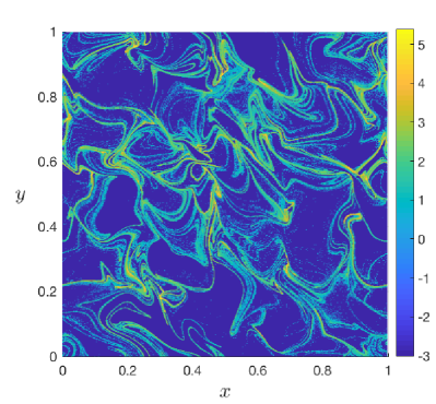
Figure 1: (Color online.) Distribution of particle positions in a two-dimensional random flow, mimicking the motion of debris on a sea surface. The density is inhomogeneous on length scales much larger than the correlation length $\xi$ of the equations of motion ($\xi=0.05$ in this illustration). The colour bar indicating density is in decimal log scale.

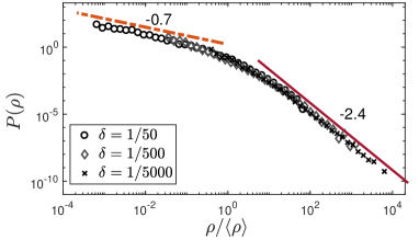
Figure 2: PDF of the particle density for the model illustrated in figure 1. There were $10^{7}$ particles, and the densities were evaluated using square regions of size $\delta$, much smaller than the correlation length $\xi=0.05$, and normalised by their mean value $\langle\rho\rangle$. The two asymptotes correspond to power laws with exponent $\alpha\approx 0.7$ (low densities) and $\beta\approx 2.4$ (high densities).

The existence of a power-law at high densities is not very surprising, because it is consistent with the notion that chaotic dynamical systems can have fractal invariant measures Ott02 ; Gra+83 . The occurrence of a power-law distribution at low densities, as documented in figure 2, is a distinct phenomenon which deserves to be understood. In this paper we describe a general approach to understanding the sparse regions of the phase space of a broad class of complex dynamical systems. We show that there is a general mechanism explaining why the sparse regions can have a power-law distribution of density, and discuss examples where the exponent $\alpha$ of the low-density distribution, which we term the lacunarity exponent, can be estimated. In support of our claim that the effect is widely observable, we note that evidence which supports equation (1) has previously been presented in numerical and experimental studies of a few different systems with quite disparate equations of motion (the examples that we know about, Bec+07 ; Lar+09 ; Pra+17 ; Kaw+17 , are discussed below).

The term ‘lacunarity’ was introduced as a notion for characterising fractal sets by Mandelbrot Man82 , and various approaches to defining lacunarity have been explored Gef+83 ; Plo+96 , measuring the spatial inhomogeneity of a set (which need not be a fractal). Our definition of the lacunarity exponent characterises a very strong type of inhomogeneity, which we claim is a robust and widely observable phenomenon.

In order to explain the existence of the lacunarity exponent we consider the simplest model for which we have observed its existence. This is the correlated random walk, defined by

$$x_{n+1}=x_{n}+f_{n}(x_{n})$$ (2)

where the $f_{n}(x)$ are random, smooth functions, with $\langle f_{n}(x)\rangle=0$ and a correlation function of the form

$$\langle f_{n}(x)f_{n^{\prime}}(x^{\prime})\rangle=\delta_{nn^{\prime}}\epsilon^{2}\xi^{2}\exp\left(-\frac{(x-x^{\prime})^{2}}{2\xi^{2}}\right)\ ,$$ (3)

where $\xi$ is the correlation length. This one-dimensional model is chaotic (that is, has a positive Lyapunov exponent) when $\epsilon$ exceeds a critical value $\epsilon_{\rm c}\approx 1.553$ Wil+03 . In figure 3 we plot the PDF of the density of final points for this model after $N=100$ iterations, obtained by iterating a very dense distribution of initial points. The density $\rho$ in our numerical studies of this model is defined empirically, using the number of trajectories ${\cal N}$ in a randomly chosen interval of length $\delta$, by writing $\rho={\cal N}/\delta$. The PDF of the density, $P(\rho)$, was determined by dividing the range of $x$ into bins of length $\delta$ (for the two-dimensional system illustrated in figures 1 and 2 we divided the coordinate space into squares of side $\delta$, and defined $\rho={\cal N}/\delta^{2}$). The plot of the distribution shows that there are also two power-law asymptotes for this model, which are compared with theoretical predictions for the exponents $\alpha$ and $\beta$ which will be described below. We find that the exponents of both power laws approach limits as the number of iterations $N$ increases and as the size of the interval $\delta$ decreases, provided that the number of trajectories is sufficiently large (i.e. ${\cal N}\gg 1$). Figure 3 contains data for four different values of $\delta$. We used a periodic realisation of the random functions $f_{n}(x)$, with period $L=5$, and with correlation length $\xi=0.5$. The total number of trajectories was $5\times 10^{4}$, initially uniformly scattered over $[0,L]$. The exponents change continuously as the parameters of the model are varied.

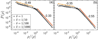
Figure 3: PDF of the density for the correlated random walk map, equations (1) and (2), for two different values of $\epsilon$, namely $\epsilon=1.5\epsilon_{c}$ (a) and $\epsilon=1.9\epsilon_{c}$ (b), which are expressed as multiples of the critical value $\epsilon_{\rm c}$ where the Lyapunov exponent vanishes. The PDF of the density exhibits a power-law, with different exponents, in both the low- and high-density limits. The dashed line and solid line correspond to the theoretical predictions given by Eq. (7) and Eq. (10), respectively.

Now we present arguments supporting the existence of these power-laws. For clarity, we start by considering the simplest case, which is a chaotic map in one dimension, such as that described by equations (2) and (3). If $\rho_{N}(x)$ is the density of particles after $N$ iterations, the density at $x$ after $N+1$ iterations is

$$\rho_{N+1}(x)=\sum_{j=1}^{K}\left|\frac{\partial x_{N+1}}{\partial x_{N}}\right|^{-1}_{x_{j}}\rho_{N}(x_{j})$$ (4)

where the $x_{j}$ are the $K$ pre-images of $x$ at iteration $N$.

Because of the un-predictability of chaotic motion, we apply probabilistic methods. If there is only one pre-image, the value of $\rho$ is simply multiplied by $|\partial x^{\prime}/\partial x|^{-1}$, which we treat as if it is a random factor. If there are multiple pre-images, the sum components are likely to be very different in magnitude, so that the density will be dominated by the largest term PPW18 . Because of the multiplicative nature of the density mapping, the different branches can have dramatic differences in magnitude, so that approximating the sum by its largest term is a valid approximation when considering the limit of very high densities. The statistical treatment of the map from $\rho_{N}$ to $\rho_{N+1}$ simplifies in both the low- and high-density limits, leading to a power-law for the probability density $P(\rho)$. We consider these in turn.

We formulate our argument for maps which have Markovian properties. First we assume that the density at $x$ is very small. At the next iteration, where $x$ is mapped to $x^{\prime}$, there may be other trajectories which reach $x^{\prime}$. In general, the number $K$ of pre-images of $x^{\prime}$ may be regarded as a random number, with a probability $P_{K}$ (note that $K$ is an odd number for continuous maps).

Consider how very small values of the density $\rho(x)$ are realised. Because the map is assumed to be chaotic, the values of factors by which the density is changed at each iteration, namely $|\partial x^{\prime}/\partial x|^{-1}$, are expected to be typically less than unity, implying that the density will decrease upon iteration of the map. This tendency to produce smaller densities is frustrated by the possibility of the map folding the pre-image space. In the limit as $\rho\to 0$, the occurrence of a typical folding event will increase the density to a typical value. Very small values of the density are, therefore, the result of trajectories which repeatedly escape folding. Because of the Markovian nature of a map such as equations (2) and (3), the probability of surviving for $m$ iterations without a folding event is $P_{1}^{m}$. In $m$ iterations without folding, the density changes by a factor $F_{m}$ which satisfies

$$\langle\ln F_{m}\rangle=m\bigg{\langle}\ln\biggl{|}\frac{\partial x^{\prime}}{\partial x}\bigg{|}^{-1}\biggr{\rangle}_{1}$$ (5)

where $\langle X\rangle_{1}$ is an average over trajectories which have only one pre-image. The distribution of the logarithm of the density, $X=\ln\rho$, therefore satisfies

$$P(X)\sim\exp\left(\frac{\ln\,P_{1}}{\langle\ln|\partial x^{\prime}/\partial x|^{-1}\rangle_{1}}X\right)\ .$$ (6)

This implies that there is a power-law distribution of $\rho$ of the form (1) at small values, with lacunarity exponent

$$\alpha=1-\frac{\ln\,P_{1}}{\langle\ln|\partial x^{\prime}/\partial x|^{-1}\rangle_{1}}\ .$$ (7)

In general it is extremely hard to make a theoretical calculation of either the numerator or the denominator in the expression for $\alpha$, equation (7), because of the difficulty of incorporating the condition that there is no folding into the averaging procedure, but later we shall describe a simplified version of the model contained in (2) and (3) which does allow us to give an exact expression for the exponent $\alpha$. The reasoning leading to the prediction of a power-law distribution for small values of $\rho$ is, however, very robust. We only used the assumption that there is a finite probability for a trajectory to have just one pre-image.

In the case where the density $\rho(x)$ greatly exceeds the typical value of the density, the contributions to $\rho(x^{\prime})$ from other pre-images are almost certainly negligible, so that the transformed density is $\rho^{\prime}(x^{\prime})=\rho(x)/F$, where $F=|\partial x^{\prime}/\partial x|$. The factor $F$ may be treated as a random variable with probability density $\pi(F)$. After $N$ iterations the density $\rho$ varies extremely rapidly as a function of the coordinate $x$. Let $Q_{N}(\rho)$ be the probability that the density at a given point is less than $\rho$ after $N\gg 1$ iterations. At the next iteration, the cumulative probability depends upon the statistics of the sensitivity factor $F(x)=|\partial x_{N+1}/\partial x_{N}|$: regions of density $\rho$ become regions of density $\rho^{\prime}=\rho/F$, and intervals of length ${\rm d}x$ become intervals of length ${\rm d}x^{\prime}=F{\rm d}x$. Because $\rho(x)$ fluctuates very rapidly as a function of $x$, a small region of length $\delta x$ has a range of different values of $\rho$, with cumulative weight $Q_{N}(\rho)\delta x$. At the next iteration, the image of this interval has width $\delta x^{\prime}=F\delta x$, with cumulative weight $\delta x^{\prime}Q_{N}(F\rho)$. Integrating over the distribution of $F$, the cumulative probability of $\rho$ is therefore iterated as follows:

$$Q_{N+1}(\rho)=\int_{0}^{\infty}{\rm d}F\ \pi(F)\,F\,Q_{N}(F\rho)\ .$$ (8)

Seeking a steady-state solution for the PDF of the density of the form $P(\rho)=\frac{{\rm d}Q}{{\rm d}\rho}\sim\rho^{-\beta}$ we find that

$$1=\int_{0}^{\infty}{\rm d}F\ \pi(F)\,F^{2-\beta}$$ (9)

which is an implicit equation for the high-density exponent, $\beta$.

The existence of a power-law distribution of density in the high density limit can be related to the fractal properties of the attractor. One characterisation of the fractal properties is achieved by considering the expectation value $\langle{\cal N}(\varepsilon)\rangle$ of the number of trajectories within an interval of length $\varepsilon$ centred on a randomly chosen test trajectory: $\langle{\cal N}\rangle\sim\varepsilon^{D_{2}}$, where $D_{2}$ is termed the correlation dimension Gra+83 . In Wil+12 , it was shown that $D_{2}$ satisfies a relation closely related to (9), implying that

$$\beta=D_{2}+2\ .$$ (10)

Our discussions have assumed that the empirical density, defined by writing $\rho={\cal N}/\delta$ for finite $\delta$, is compatible with the density defined mathematically by taking $\delta\to 0$. This is not guaranteed, because as the number of iterations of the map increases, the sensitivity of the final position $x_{N}$ to the initial coordinate increases exponentially with the number of iterations, $N$. This implies that, unless $N$ is small, the empirically determined density is given by an average of the value of $\rho(x)$ which fluctuates very rapidly over an interval. The mean number of trajectories in a randomly chosen interval of length $\varepsilon$ has the scaling $\langle{\cal N}\rangle\sim\varepsilon^{D_{1}}$, where $D_{1}$ is termed the information dimension. If the distribution of $P(\rho)$ has a finite mean value, we expect that the number of trajectories in an interval is proportional to the length of that interval, implying that $D_{1}=1$. The mean value is finite if $\beta>2$. Equation (10) implies that this condition is satisfied whenever $D_{2}>0$. This holds whenever the motion is chaotic (that is, the map has positive Lyapunov exponent Wil+12 ).

In the general case the equation for the exponent $\alpha$, (7), is not susceptible to further analysis and must be solved numerically. We describe one special case of the map (2) where an explicit expression for $\alpha$ has been obtained. Consider the map

$$x_{n+1}=x_{n}+F(x-\phi_{n})$$ (11)

where $F(x)=F(x+1)$ is a periodic function, and where $\phi_{n}$ is a random number which is uniformly distributed on $[0,1]$. We consider the case where $F(x)$ is piecewise linear:

$$F(x)=\left\{\begin{array}[]{cc}gx&0\leq x\leq\frac{1}{2}\cr g(1-x)&\frac{1}{2}\leq x\leq 1\end{array}\right.$$ (12)

(where $g>0$), so that the function $F$ is continuous and piecewise linear, with gradients $\pm g$. For this model, the forward map (11) has gradients with magnitude $1+g$ or $1-g$, both with with probability $\frac{1}{2}$. The Lyapunov exponent of the model is

$$\lambda=\frac{1}{2}\left[\ln|g+1|+\ln|g-1|\right]$$ (13)

so that the model is chaotic ($\lambda>0$) when $g>\sqrt{2}$.

Now consider how to compute the exponents $\alpha$ and $\beta$ which characterise the low- and high-density limits of the PDF of $\rho$. When $g>1$, a point may have multiple pre-images. When $g<3$, any point has either a single pre-images, with probability $P_{1}$, or else three pre-images, with probability $P_{3}=\frac{(g-1)}{2}$. For this model, points which have just one pre-image all have the same expansion factor, namely $g+1$, so that the low-density exponent is

$$\alpha=1+\frac{\ln(1-P_{3})}{\ln(g+1)}=1+\frac{\ln[(3-g)/2]}{\ln(g+1)}\ .$$ (14)

Equation (9) determining the high-density exponent, $\beta=D_{2}+2$, becomes

$$(g+1)^{(2-\beta)}+(1-g)^{(2-\beta)}=2,$$ (15)

which is an implicit equation that must be solved numerically. Comparing equations (14) and (15), it is clear that there is no simple relationship between the exponents $\alpha$ and $\beta$.

We tested our predictions numerically. Figure 3 shows a comparison between the numerically computed density PDF and the values of the exponents obtained from (7) and (10). For $\epsilon/\epsilon_{\rm c}=1.5$, these equations predict $\alpha=0.49$ and $\beta=2.33$ respectively, whereas for $\epsilon/\epsilon_{\rm c}=1.9$, they predict $\alpha=0.35$ and $\beta=2.55$, in very good agreement with the data in figure 3. Figure 4 shows the numerically determined PDF of the piecewise linear model, comparing the exponents with (14) and the solution of (15). We can see there is clear evidence for a power-law at both high and low densities, confirming the existence of the lacunarity exponent, in agreement with the theory.

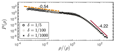
Figure 4: PDF of the density for the piecewise linear correlated random walk map, Eqs. (11) and (12), with $g=\frac{7}{4}$, where (14) and (15) give $\alpha=0.54$ (dashed line) and $\beta=4.22$ (solid line), respectively.

We mentioned in the introduction that power-law distributions of small densities had been observed in a variety of other contexts. Bec et al. Bec+07 showed that the density of inertial particles in simulations of three-dimensional turbulence has a lower-law at low densities. Larkin et al. Lar+09 have exhibited a density distribution for particles advected on the surface of a turbulent flow in a water tank. The density distribution shows two power-laws, at high and low densities. Kawagoe et al. Kaw+17 discuss the distribution of weights for a model of random ‘trails’. The distribution is asymptotic to a power-law in the limit where the weight of a trail approaches zero, and the effect is quite distinct from the growth of voids observed close to the directed percolation transition Hub+95 . Finally, the present authors previously reported Pra+17 data quite closely related to figure 3, showing high- and low-density power laws for a one-dimensional model of inertial particles. These observations concern models for the distribution of particles with quite different equations of motion, in different numbers of space dimensions. With the exception of Kaw+17 , which uses an exact solution for a specific model, these papers do not offer a clear explanation for the power-law density distribution. This begs the question as to whether there is a common mechanism which implies power-law behaviour.

The argument that we presented for the existence of the lacunarity exponent in the one-dimensional case is readily extended to a wide range of chaotic and random dynamical systems. There are two essential elements to the argument, embodied in equations (5) and (6) respectively, which can be generalised. Firstly, there must be a finite fraction of trajectories for which the volume of the pre-image of a small neighbourhood contracts exponentially as we go backwards in time. Secondly, there must be a mechanism which ensures that the pre-images do not continue to contract indefinitely, so that the sequence of contractions is broken. If the probability that this mechanism does not occur decreases exponentially as we go backwards in time, then the argument supporting equation (7) implies that $P(\rho)$ has a power-law distribution as $\rho\to 0$. In the case of the one-dimensional map, the mechanism for breaking the series of pre-image contractions is the existence of multiple pre-images.

These arguments apply directly to most of the previously reported examples, Bec+07 ; Lar+09 ; Kaw+17 ; Pra+17 . The exponential reduction of density for a single trajectory as a function of the number of iterations is a feature of all these systems: in most cases it is a result of the exponential separation of nearby trajectories, but in Kaw+17 it is the result of trajectories randomly splitting, reducing the weight in each daughter trajectory. In all of the examples in Bec+07 ; Lar+09 ; Kaw+17 ; Pra+17 except Lar+09 , the different trajectories can have multiple pre-images, and the probability of avoiding trajectories crossing or combining may be assumed to decrease exponentially as a function of time. The system considered by Larkin et al. Lar+09 involving particles floating on the surface of a liquid which is undergoing a turbulent or complex flow, is different: the equation of motion is $\dot{\mbox{\boldmath$x$}}=\mbox{\boldmath$u$}(\mbox{\boldmath$x$},t)$, with a random velocity field $\mbox{\boldmath$u$}(\mbox{\boldmath$x$},t)$. This system has a unique time-reversed motion. In this case a different mechanism for breaking the contraction of the pre-images may play a role. The pre-images of a small disc can expand in one direction, while their area contracts. The exponential contraction of the pre-image area breaks down when stretching makes its extent too large, so the linear approximation becomes inappropriate. In our numerical illustration of a two-dimensional flow, figures 1 and 2, we used a simplified model

$${\mbox{\boldmath$x$}}(t+\Delta t)={\mbox{\boldmath$x$}}(t)+\mbox{\boldmath$u$}(\mbox{\boldmath$x$},t)\Delta t\ .$$ (16)

The velocity field was constructed by writing $\mbox{\boldmath$u$}=\mbox{\boldmath$\nabla$}\wedge\mbox{\boldmath$\psi$}+\eta\mbox{\boldmath$\nabla$}\phi$ where $\phi$ and $\psi$ have the same isotropic, homogeneous statistics and are independent of each other, and where $\eta$ is a parameter which controls the compressibility. In the simulations we used $\eta=0.5$ and a large value of $\Delta t$ ($\Delta t=0.5$) to ensure that the forward and time-reversed flows have different statistical properties.

In summary, we have argued that dynamical processes can produce regions of extremely sparse trajectories, characterised by a power-law distribution of density, parametrised by the lacunarity exponent, $\alpha$. This property of having a power-law distribution of small densities is complementary to the power-law distribution of high-density regions, which is associated with a fractal dimension. We have described a robust mechanism explaining the existence of this power law, and shown how the exponent can be computed for one-dimensional systems. The existence of a lacunarity exponent is consistent with existing observations on a variety of dynamical systems, and it may prove to be a widely observable and quantifiable property.

Acknowledgements. The authors are grateful to the Kavli Institute for Theoretical Physics for support, where this research was supported in part by the National Science Foundation under Grant No. PHY11-25915.

Author email addresses:

marc.pradas@open.ac.uk

alain.pumir@ens-lyon.fr

greg.huber@czbiohub.org

m.wilkinson@open.ac.uk

References

- (1) B. T. J. Jones, V. J. Martinez, E. Saar and V. Trimble, Rev. Mod. Phys., 76, 1211-66, (2005).
- (2) B. J. Elmegreen and D. M. Elmegreen, Astrophys. J., 121, 1507-11, (2001).
- (3) L. Yu, Q. Chen and E. Ott, Phys. Rev. Lett., 53, 102, (1991).
- (4) J. C. Sommerer and E. Ott, Science, 259, 335-39, (1993).
- (5) A. Cózara, F. Echevarríaa, J. I. Gonz lez-Gordilloa, X. Irigoienb, B. Úbedaa, S. Hernández-Leónd, . T. Palmae, Sandra Navarrof, J. Garc a de Lomasa, A. Ruizg, M. L. Fernández de Puellesh, and C. M. Duartei, PNAS, 111, 10239-44, (2014).
- (6) Y. Chen, PLoS One, 6, e24791, (2011).
- (7) R. A. Shaw, Ann. Rev. Fluid Mech., 35, 183-227, (2003).
- (8) B. B. Mandelbrot, The Fractal Geometry of Nature, Freeman, San Francisco, (1982).
- (9) K. Falconer, Fractal Geometry: mathematical foundations and applications, Wiley, New York, (1990).
- (10) E. Ott, Chaos in Dynamical Systems, 2nd edition, Cambridge: University Press, (2002).
- (11) P. Grassberger and I. Procaccia, Physica D, 9, 189-208, (1983).
- (12) J. Bec, L. Biferale, M. Cencini, A. Lanotte, S. Musacchio, and F. Toschi, Phys. Rev. Lett., 98, 084502, (2007).
- (13) J. Larkin, M. M. Bandi, A. Pumir and W. I. Goldburg, Phys. Rev. E, 80, 066301 ,(2009).
- (14) K. Kawagoe, G. Huber, M. Pradas, M. Wilkinson, A. Pumir, E. Ben-Naim, Phys. Rev. E, 96, 012142, (2017).
- (15) M. Pradas, A. Pumir, G. Huber and M. Wilkinson, Phys. A: Math. Theor., 50, 275101, (2017).
- (16) Y. Gefen, Y. Meir, B. B. Mandelbrot and A. Aharony, Phys. Rev. Lett., 50, 145-8, (1983).
- (17) R. E. Plotnick, R. H. Gardner, W. W. Hargrove, K. Prestegaard and M. Perlmutter, Phys. Rev. E, 53, 5461-8, (1996).
- (18) M. Wilkinson and B. Mehlig, Phys. Rev. E, 68, 040101, (2003).
- (19) M. Pradas, A. Pumir and M. Wilkinson, J. Phys A: Math. Theor., 51, 155002, (2018).
- (20) M. Wilkinson, B. Mehlig, K. Gustavsson and E. Werner, Eur. Phys. J. B, 85, 18, (2012).
- (21) G. Huber, M. H. Jensen and K. Sneppen, Phys. Rev. E, 52, R2133-6, (1995).