Integrated Tempering Enhanced Sampling Method as the Infinite Switching Limit of Simulated Tempering

Abstract

Fast and accurate sampling method is in high demand, in order to bridge the large gaps between molecular dynamic simulations and experimental observations. Recently, integrated tempering enhanced sampling method (ITS) has been proposed and successfully applied to various biophysical examples, significantly accelerating conformational sampling. The mathematical validation for its effectiveness has not been elucidated yet. Here we show that the integrated tempering enhanced sampling method can be viewed as a reformulation of the infinite switching limit of simulated tempering method over a mixed potential. Moreover, we demonstrate that the efficiency of simulated tempering molecular dynamics (STMD) improves as the frequency of switching between the temperatures is increased, based on the large deviation principle of empirical distributions. Our theory provides the theoretical justification of the advantage of ITS. Finally, we illustrate the utility of the infinite switching simulated tempering method through several numerical examples.

I Introduction

Molecular dynamics simulation is a powerful method for investigating microscopic biochemical systems. However, when the system contains barriers due to energy or entropy, direct molecular dynamics simulation will lead to a very high computational cost. Therefore, people turn to use the enhanced sampling method, sacrificing the real dynamic information in order to capture the desired Gibbs distribution. Until now, sampling methods have already been successfully applied in multiple disciplines including statistical physics, chemical physics, Bayesian statistics, machine learning, and related areas.

The efficiency of the sampling approach highly depends on the convergence rate to the thermodynamic equilibrium. Tempering schemes, such as simulated tempering molecular dynamics (STMD) Marinari and Parisi (1992); Kerler and Rehberg (1994) and replica exchange molecular dynamics (REMD) Hansmann (1997); Sugita and Okamoto (1999); Earl and Deem (2005), were developed and are among the most popular methods to overcome the metastability and to enhance the convergence to equilibrium, thanks to their effectiveness and simplicity to use. The basic idea of both is to use one or more artificial high temperatures to accelerate exploration of the conformational space, while using the physical temperature to sample the desired physical observable. The interaction between different temperatures is designed so to guarantee the unbiasedness of the estimation. These two methods are quite comparable to each other. STMD gives a higher rate of delivering the system between different temperature states as well a higher rate of traversing the energy space Zhang and Ma (2008), but requires the estimation of partition function first.

Another tempering algorithm named “integrated tempering enhanced sampling” (ITS), which was recently introduced by Gao Gao (2008), uses a temperature-biased effective potential energy to run the MD simulation and has been successfully applied to various biochemical examples Yang et al. (2009, 2015). Noting that ITS also uses auxiliary temperatures to accelerate the convergence, it is desirable to compare it with previous methods, and find out why it performs better in many cases, which has not been studied theoretically to the best of our knowledge.

As one of the main results in this paper, we discover that the integrated tempering enhance sampling method is in fact a reformulated version of the infinite switching limit of STMD, that is, the limit of the simulated tempering when the attempt switching frequency goes to infinity. Moreover, we show that as the switching rate in STMD increases, the empirical measure converges faster towards stationary distribution, using the large deviation principle; and thus the sampling efficiency of STMD increases as the switching frequency increases. Combining the two theoretical findings, we justify the efficiency of ITS over conventional STMD. Finally, we compare the infinite switching STMD against the normal STMD with two numerical examples: an artificial high dimensional system and a more realistic Lennard-Jones example Dellago et al. (1999) with 16 atoms. The numerical results validate our theoretical findings.

Our study of the switching rate of the STMD is closely related to the recent progress in understanding the swapping frequency of tempering schemes, started with replica exchange methods. For REMD, it has been discovered through numerical examples that the sampling efficiency increases when the frequency of swapping of temperatures is pushed up to infinity Sindhikara et al. (2008); but directly increasing the swapping rate to reach this limit is computationally infeasible, as many swaps are needed per MD step. A breakthrough was made in Plattner et al. (2011); Dupuis et al. (2012) which proposed an explicit way to reach this limit and also proved that indeed the sampling efficiency increases in such limit. A natural reformulation of infinite swapping REMD was later proposed in Lu and Vanden-Eijnden (2013) which leads to an easy implementation as a simple patch to conventional molecular dynamics. For multiple temperatures, an efficient implementation based on ideas of multiscale integrator was also proposed for infinite swapping REMD Yu et al. (2016); Lu and Vanden-Eijnden (2017), which leads to practical applications in sampling configurational space of large biomolecules. We note that increasing the switching rate in the simulated tempering has been mentioned in Lu and Vanden-Eijnden (2017) and Martinsson et al. under a general framework of viewing tempering schemes as MD process augmented by jumping processes, without much details in particular the connection with ITS.

In the remaining article, we will first recall the simulated tempering molecular dynamics as a stochastic process in Sec. II. We will justify using a large switching frequency via large deviation principle for the empirical distribution in Sec. III with detailed derivation given in the Appendix. Infinite switching limit of STMD and its reformulation are derived and generalized in Sec. IV and V. The identification of ITS and infinite switching STMD is given and discussed in Sec. VI, followed by numerical examples in Sec. VII. Some conclusive remarks are given in Sec. VIII.

II Simulated tempering molecular dynamics

We begin by recalling the simulated tempering molecular dynamics. For the sake of simplicity we will first discuss the algorithm for system governed by overdamped Langevin equations (i.e., when inertia can be neglected). More general dynamics will be discussed in Sec. V. Consider

$$\dot{\bm{x}}=\bm{f}(\bm{x})+\sqrt{2\beta^{-1}}\,\bm{\eta},$$ (1)

where $\bm{x}\in\mathbb{R}^{3n}$ denotes the configuration of the system with $n$ particles, $\bm{f}(\bm{x})=-\nabla V(\bm{x})$ is the force associated with the potential $V(\bm{x})$, $\beta=1/k_{B}T$ is the inverse temperature, and $\bm{\eta}$ is a $3n$-dimensional white-noise with independent components. We choose a unit system so that the friction coefficient becomes one for notational simplicity. Eq. (1) is consistent with the Boltzmann equilibrium probability density

$$\rho_{\beta}(\bm{x})=Z_{\beta}^{-1}e^{-\beta V(\bm{x})},$$ (2)

where the normalization constant $Z_{\beta}=\int_{\mathbb{R}^{3n}}e^{-\beta V(\bm{x})}d\bm{x}$ is the partition function.

Assuming we only take two temperatures in simulated tempering (the generalization to more temperatures will be considered in Sec. V), we replace (1) by

$$\dot{\bm{x}}=\bm{f}(\bm{x})+\sqrt{2\beta^{-1}(t)}\,\bm{\eta},$$ (3)

where the inverse temperature $\beta(t)$ now attempts switches between the physical and the artificial temperatures with frequency $\nu$, and the attempted switch from $\beta_{1}$ to $\beta_{2}$ are accepted with probability

$$g_{\beta_{1}\beta_{2}}(\bm{x})=\min\left(\frac{n_{2}\,e^{-\beta_{2}V(\bm{x})}}{n_{1}\,e^{-\beta_{1}V(\bm{x})}},1\right),$$ (4)

where $n_{1}$ and $n_{2}$ are some weighting parameters that will be further discussed below.

Note that in the simulated tempering overdamped dynamics, both the configuration $\bm{x}$ and the inverse temperature $\beta$ are dynamical variables: $\bm{x}$ follows (3), $\beta$ follows a jump process and the two dynamics are coupled. To understand the dynamics, it is useful to consider its infinitesimal generator, given by (we use $\beta^{\prime}$ to denote the temperature other than $\beta$, namely $\beta^{\prime}=\beta_{2}$ if $\beta=\beta_{1}$ and vice versa)

$$(\mathcal{L}^{\nu}u)(\bm{x},\beta)=-\nabla V(\bm{x})\cdot\nabla_{\bm{x}}u(\bm{x},\beta)+\beta^{-1}\Delta_{\bm{x}}u(\bm{x},\beta)\\ -\nu g_{\beta,\beta^{\prime}}(\bm{x})u(\bm{x},\beta)+\nu g_{\beta^{\prime},\beta}(\bm{x})u(\bm{x},\beta^{\prime})$$ (5)

for a smooth function $u:\mathbb{R}^{3n}\times\{\beta_{1},\beta_{2}\}\to\mathbb{R}$. This means that the evolution of a physical observable $u$ under the dynamics is given by

$$\mathbb{E}\bigl{(}u(\bm{x}(t+\delta t),\beta(t+\delta t))\mid\bm{x}(t),\beta(t)\bigr{)}=u(\bm{x}(t),\beta(t))\\ +\delta t(\mathcal{L}^{\nu}u)(\bm{x}(t),\beta(t))+o(\delta t),$$ (6)

or equivalently, the density $\rho$ of $(\bm{x},\beta)$ evolves under the adjoint operator:

$$\partial_{t}\rho(t,\bm{x},\beta) =\bigl{(}\mathcal{L}^{\nu}\bigr{)}^{\dagger}\rho(t,\bm{x},\beta)$$ (7)

$$=\Delta V(\bm{x})\cdot\rho(t,\bm{x},\beta)+\nabla V(\bm{x})\cdot\nabla_{\bm{x}}\rho(t,\bm{x},\beta)$$

$$\qquad+\beta^{-1}\Delta_{\bm{x}}\rho(t,\bm{x},\beta)-\nu g_{\beta,\beta^{\prime}}\rho(t,\bm{x},\beta)$$

$$\qquad+\nu g_{\beta^{\prime},\beta}\rho(t,\bm{x},\beta^{\prime}).$$

For the infinitesimal generator, the first two terms on the right hand side of (5) correspond to the overdamped dynamics (3) while the last two terms correspond to the jump process of $\beta$, $-\nu g_{\beta,\beta^{\prime}}(\bm{x})$ being the rate of switching from temperature $\beta$ to $\beta^{\prime}$, and $\nu g_{\beta^{\prime},\beta}(\bm{x})$ is the rate of switching to $\beta$ from the other temperature $\beta^{\prime}$ (attempt switching frequency adjusted by the acceptance rate).

It is straightforward to check the equilibrium distribution of the coupled dynamics of $(\bm{x},\beta)$, as the stationary solution of (7) is given by

$${\varrho}(\bm{x},\beta)=\frac{n_{1}e^{-\beta_{1}V(\bm{x})}\delta_{\beta,\beta_{1}}+n_{2}e^{-\beta_{2}V(\bm{x})}\delta_{\beta,\beta_{2}}}{n_{1}Z_{\beta_{1}}+n_{2}Z_{\beta_{2}}},$$ (8)

where $\delta_{\beta,\beta_{1}}$ denotes the Kronecker delta: $\delta_{\beta,\beta_{1}}=1$ if and only if $\beta=\beta_{1}$. This is nothing but a weighted average of Boltzmann densities at temperatures $\beta_{1}$ and $\beta_{2}$, with weight $n_{1}Z_{\beta_{1}}$ and $n_{2}Z_{\beta_{2}}$ respectively. On each fixed temperature, the distribution is generated by the ordinary molecular dynamics and thus follows Boltzmann distribution; meanwhile, at each fixed configuration, the proportion of the two temperatures is given by

$$\omega_{j}(\bm{x})=\frac{n_{j}e^{-\beta_{j}V(\bm{x})}}{n_{1}e^{-\beta_{1}V(\bm{x})}+n_{2}e^{-\beta_{2}V(\bm{x})}},\quad j=1,2$$ (9)

as determined by the acceptance probability (4). Therefore, (3) together with the jumping process of $\beta$ samples the $\varrho(\bm{x},\beta)$ as the equilibrium distribution.

Summing $\varrho(\bm{x},\beta)$ over $\beta$ then gives the marginal equilibrium density for the configuration position alone

$$\varrho(\bm{x})=\varrho(\bm{x},\beta_{1})+\varrho(\bm{x},\beta_{2})　=　\frac{n_{1}e^{-\beta_{1}V(\bm{x})}+n_{2}e^{-\beta_{2}V(\bm{x})}}{n_{1}Z_{\beta_{1}}+n_{2}Z_{\beta_{2}}},$$ (10)

which is a weighted average of the Boltzmann densities at the two temperatures $\beta_{1}$ and $\beta_{2}$. As a result the ensemble average at the physical temperature ($\beta_{1}$) of any observable $A(\bm{x})$ can be estimated from

$$\langle A\rangle_{\beta_{1}} \equiv\int_{\mathbb{R}^{3n}}A(\bm{x})\rho_{\beta_{1}}(\bm{x})\,\mathrm{d}\bm{x}$$ (11)

$$=\frac{n_{1}Z_{\beta_{1}}+n_{2}Z_{\beta_{2}}}{n_{1}Z_{\beta_{1}}}\int_{\mathbb{R}^{3n}}A(\bm{x})\,\omega_{1}(\bm{x})\varrho(\bm{x})\,\mathrm{d}\bm{x}$$

$$=\biggl{(}\int_{\mathbb{R}^{3n}}\omega_{1}(\bm{x})\varrho(\bm{x})\,\mathrm{d}\bm{x}\biggr{)}^{-1}\int_{\mathbb{R}^{3n}}A(\bm{x})\,\omega_{1}(\bm{x})\varrho(\bm{x})\,\mathrm{d}\bm{x}$$

$$\approx\dfrac{\displaystyle\lim_{T\to\infty}\frac{1}{T}\int_{0}^{T}A(\bm{x}(t))\,\omega_{1}(\bm{x}(t))\,\mathrm{d}t}{\displaystyle\lim_{T\to\infty}\frac{1}{T}\int_{0}^{T}\omega_{1}(\bm{x})\,\mathrm{d}t}\,,$$

where we have used that the ensemble average equals to the time average thanks to ergodicity. Note that in principle we shall use two independent realization to estimate the numerator and denominator on the right hand side of (11) to get an unbiased estimator, while in practice the bias is well-controlled and the variance of the estimator usually dominates the error.

Note that the above holds for arbitrary positive weighting factors $n_{1}$ and $n_{2}$; while the sampling efficiency of the method depends on the choice. The conventional wisdom in simulated tempering method is to choose $n_{1}$ and $n_{2}$ according to the partition function:

$$n_{1}=Z_{\beta_{1}}^{-1}\qquad\text{and}\qquad n_{2}=Z_{\beta_{2}}^{-1}.$$ (12)

With this choice, we have

$$\varrho(\bm{x},\beta)=\frac{1}{2}\rho_{\beta_{1}}(\bm{x})\delta_{\beta,\beta_{1}}+\frac{1}{2}\rho_{\beta_{2}}(\bm{x})\delta_{\beta,\beta_{2}}$$ (13)

and thus the sampler spends equal amount time at the two temperatures. It is also possible to choose different $n_{i}$ to emphasize one of the temperatures. Of course, the partition functions $Z_{\beta_{i}}$ are not known a priori, and hence the usual approach is to start with some initial guess of the weighting factors and then adaptively adjust them on-the-fly using an iterative method, see e.g., Park and Pande (2007); Gao (2008); Tan (2017); Martinsson et al. . In what follows, we will mainly focus on the choice of the switching frequency $\nu$, and thus for the simplicity of discussion, we will assume that $n_{i}$ are fixed during the sampling process and only make some remarks about adjusting $n_{i}$ afterwards.

III Large deviation principle for empirical measure

As we have discussed above, for any choice of the switching frequency $\nu$, the trajectory $(\bm{x}^{\nu},\beta^{\nu})$ (we put superscript $\nu$ to emphasize the $\nu$ dependence) of the simulated tempering overdamped dynamics can be used to sample the equilibrium distribution (8). In particular, the empirical distribution of the trajectory, defined blow,

$$\lambda_{T}^{\nu}\equiv\frac{1}{T}\int_{B}^{B+T}\delta_{(\bm{x}^{\nu}(t),\beta^{\nu}(t))}\,\mathrm{d}t$$ (14)

will converge to the equilibrium distribution $\varrho$ as $T\to\infty$. Note here $\delta_{(\bm{x},\beta)}$ denotes the Dirac delta function, that is the point mass function at $(\bm{x},\beta)$, and $B$ is any fixed burn-in time (which for simplicity will be taken as $B=0$ in the numerical experiments).

To discuss the choice of $\nu$, it is important then to quantify the speed of convergence of the empirical distribution (14) to the equilibrium: A better $\nu$ will correspond to faster convergence and thus less simulation length of the trajectory. To quantify this convergence for STMD, the theoretical tool we will use is the large deviation principle for the empirical measure of stochastic processes. We will discuss the idea and conclusion of the large deviation principle below, while defer the rigorous definition and derivation to the Appendix.

When $T$ becomes large, the empirical distribution is expected to be very close to the equilibrium. The large deviation principle quantifies the probability that the empirical distribution is still far away from the equilibrium: more specifically, let the probability of the empirical distribution being equal to $\mu$ is on the order of $O(e^{-I^{\nu}(\mu)T})$, with a rate functional, specific form given below, $I^{\nu}(\mu)\geq 0$, and only vanish when $\mu$ is the equilibrium distribution $\varrho$. This in particular tells us that as $T\to\infty$, the likelihood that empirical distribution is deviated away from the equilibrium is exponentially small, for which the functional $I^{\nu}$ quantifies the rate of the exponential decay. Hence a larger rate function indicates faster rate of convergence.

To specify the rate functional, let $\mu$ be a probability measure on $\mathbb{R}^{3n}\times\{\beta_{1},\beta_{2}\}$ with smooth density and define $\theta(\bm{x},\beta):=[d\mu/d\varrho](\bm{x},\beta)$, the ratio of the probability density of $\mu$ and the equilibrium distribution. For the simulated tempering process with switching frequency $\nu$, the large deviation rate function for the empirical measure converging to the stationary one is given by

$$I^{\nu}(\mu)=J_{0}(\mu)+\nu J_{1}(\mu),$$ (15)

where

$$J_{0}(\mu) =\sum_{\beta}\int\dfrac{1}{4\theta(\bm{x},\beta)^{2}}\left[\beta^{-1}|\nabla_{x}\theta(\bm{x},\beta)|^{2}\right]\mu(\,\mathrm{d}\bm{x},\beta);$$ (16)

$$J_{1}(\mu) =\tfrac{1}{2}\sum_{\beta}\int g_{\beta\beta^{\prime}}(\bm{x})\biggl{[}1-\sqrt{\dfrac{\theta(\bm{x},\beta^{\prime})}{\theta(\bm{x},\beta)}}\biggr{]}^{2}\mu(\,\mathrm{d}\bm{x},\beta).$$ (17)

Note that $J_{1}$ is non-negative and hence the large deviation rate functional is a pointwise monotonic function in $\nu$. Thus, we conclude from that a larger swapping rate $\nu$ corresponds to a faster convergence of the empirical distribution to equilibrium.

IV Infinite switching limit

As shown in the last section, the higher the switching rate $\nu$ is, the faster the convergence of the empirical distribution, and thus the sampling of the simulated tempering overdamped dynamics. On the other hand however, a large $\nu$ value requires one to make many swapping attempts, which slows down the actual simulation. To resolve this problem, the key is that the limit when $\nu\to\infty$ can be taken explicitly. This observation is first made for replica exchange dynamics in Dupuis et al. (2012). As for simulated tempering, when the switching frequency between the temperatures $\nu\to\infty$, the dynamics (3) converges to the following

$$\dot{\bm{x}}=\bm{f}(\bm{x})+\sqrt{2(\beta_{1}^{-1}\omega_{1}(\bm{x})+\beta_{2}^{-1}\omega_{2}(\bm{x}))}\bm{\eta}$$ (18)

where the effective temperature $T(\bm{x})=\beta_{1}^{-1}\omega_{1}(\bm{x})+\beta_{2}^{-1}\omega_{2}(\bm{x})$ is a weighted average of $T_{1}=\beta_{1}^{-1}$ and $T_{2}=\beta_{2}^{-1}$, where the weight as a function of $\bm{x}$ is given by (9). Intuitively, this can be understood as with fixed configuration $\bm{x}$ the proportion of time the trajectory spends at temperature $\beta_{j}$ is given by $\omega_{j}(\bm{x})$, and thus the effective temperature is given by a weighted average of the two temperatures.

The Fokker-Planck equation for the probability density of $\bm{x}(t)$ corresponding to (18) can be written as

$$\partial_{t}\rho(t)=\operatorname{div}\bigl{(}\mathbb{B}(\rho(t)\operatorname{grad}U+k_{B}T_{1}\operatorname{grad}\rho(t))\bigr{)},$$ (19)

where we have defined the effective potential

$$U(\bm{x})=-\beta_{1}^{-1}\ln\varrho(\bm{x})$$ (20)

and the mobility

$$\mathbb{B}(\bm{x})=\omega_{1}(\bm{x})+\beta_{1}^{-1}\beta_{2}\omega_{2}(\bm{x}).$$ (21)

It is easy to check that the stationary solution of (19) is $\exp\bigl{(}-\beta_{1}U(\bm{x}))$, which is just $\varrho(\bm{x})$ by definition of $U$.

Note that this point of view also leads to a further simplification of (18), in the spirit of Lu and Vanden-Eijnden Lu and Vanden-Eijnden (2013). We may replace $\mathbb{B}$ in the Fokker-Planck equation (19) by a constant function, which, for convenience, we will simply take to be the identity. This substitution does not affect the stationary distribution, and hence preserves the sampling property, but it changes the overdamped Langevin dynamics associated to the Fokker-Planck equation. It is easy to see that this new dynamics is given by

$$\dot{\bm{x}}=\bigl{(}\omega_{1}(\bm{x})+\beta_{2}\beta_{1}^{-1}\omega_{2}(\bm{x})\bigr{)}\bm{f}(\bm{x})+\sqrt{2\beta_{1}^{-1}}\bm{\eta}.$$ (22)

Compare with (18), the noise term is additive in (22), and it still samples the desired stationary distribution $\varrho$. Note that (22) is very similar to the original overdamped Langevin dynamics (1). The only change is a scaling factor in front of the forcing term, which involves the auxiliary (inverse) temperature $\beta_{2}$ and also the weights $\omega_{j}$, $j=1,2$. Note that in practice (22) can be implemented as an easy patch of existing codes for molecular dynamics.

V Generalizations

First, the idea in the previous section can be extended naturally to more than two temperatures. For which, the dynamics in the infinite switching limit is given by

$$\dot{\bm{x}}=\hbox{$\beta_{1}^{-1}\sum_{k}(\beta_{k}\omega_{k}(\bm{x}))\bm{f}(\bm{x})+\sqrt{2\beta_{1}^{-1}}\bm{\eta}$},$$ (23)

where we define the weight here as

$$\omega_{k}(\bm{x})=\frac{n_{k}e^{-\beta_{k}V(\bm{x})}}{\sum_{j}n_{j}e^{-\beta_{j}V(\bm{x})}},\quad k=1,\cdots,N,$$ (24)

if $N$ is the number of temperatures used. Similarly, the dynamics (23) can be viewed as the overdamped dynamics with the effective potential given by (20) where the corresponding marginal equilibrium density becomes

$$\varrho(\bm{x})　=　\frac{\sum_{j}n_{j}e^{-\beta_{j}V(\bm{x})}}{\sum_{j}n_{j}Z_{\beta_{j}}},$$ (25)

as we have

$$\nabla_{\bm{x}}U(\bm{x}) =-\beta_{1}^{-1}\frac{\nabla_{\bm{x}}\sum_{k}n_{j}e^{-\beta_{j}V(\bm{x})}}{\sum_{k}n_{j}e^{-\beta_{j}V(\bm{x})}}$$ (26)

$$=\beta_{1}^{-1}\frac{\sum_{k}\beta_{k}n_{j}e^{-\beta_{j}V(\bm{x})}\nabla V(\bm{x})}{\sum_{k}n_{j}e^{-\beta_{j}V(\bm{x})}}$$

$$=\beta_{1}^{-1}\sum_{k}\beta_{k}\omega_{k}(\bm{x})\bm{f}(\bm{x}).$$

Thus the gradient of the effective potential $U(\bm{x})$ is exactly the forcing term in (23).

The infinite switching simulated tempering can be also generalized to (underdamped) Langevin equation, rather than the overdamped Langevin dynamics (1); other thermostats can be also used. Recall the Langevin equation

$$\begin{cases}\dot{\bm{x}}=m^{-1}\bm{p},\\[5.69054pt] \dot{\bm{p}}=\bm{f}(\bm{x})-\gamma\bm{p}+\sqrt{2\gamma m\beta^{-1}}\bm{\eta},\end{cases}$$ (27)

where $m$ denotes the mass and $\gamma$ the friction coefficient, in which case the generalization of (22) reads

$$\begin{cases}\dot{\bm{x}}=m^{-1}\bm{p},\\[5.69054pt] \dot{\bm{p}}=\beta_{1}^{-1}\sum_{k}(\beta_{k}\omega_{k}(\bm{x}))\bm{f}(\bm{x})\\[4.2679pt] \qquad\qquad-\gamma\bm{p}+\sqrt{2\gamma m\beta^{-1}}\bm{\eta}.\end{cases}$$ (28)

The structure of the equation is rather similar to the overdamped case (22), the only modification compared to (27) is the scaling factor in front of the forcing term that amounts to a weighted average of the inverse temperatures.

VI Connection with integrated tempering enhanced sampling

The infinite switching limit of the simulated tempering sampling scheme is very closely related to the integrated tempering enhanced sampling (ITS) algorithm originally proposed in Gao (2008). The ITS algorithm introduces a temperature biased effective potential energy as

$$V_{\text{eff}}(\bm{x})=-\beta_{1}^{-1}\text{ln}\left(\sum_{k}n_{\beta_{k}}e^{-\beta_{k}V(\bm{x})}\right)$$ (29)

and run molecular dynamics simulation on the surface. Here $n_{\beta_{k}}$ is chosen to be some weighting factor for the temperature $\beta_{k}$. Note that this is identically the same as we have in (20) with the marginal equilibrium $\varrho(\bm{x})$ given by (25), despite a constant difference which does not matter in sense of potential energy.

As a conclusion, the ITS algorithm can be viewed as the infinite switching limit of the simulated tempering algorithm. As we discussed in Section III, the sampling efficiency of the simulated tempering method increases as $\nu\to\infty$. Thus as a corollary, the ITS algorithm is more efficient in sampling compared with the simulated tempering algorithm at a finite switching rate. This will be further demonstrated in our numerical examples in the next section.

VII Numerical examples

VII.1 Simple high dimensional example

We first consider a system in $D$ dimension moving on the following potential with $\bm{x}=(x_{0},\cdots,x_{D-1})$

$$V(\bm{x})=(1-x_{0}^{2})^{2}-\dfrac{1}{4}x_{0}+\sum_{j=1}^{D-1}\dfrac{1}{2}\lambda_{j}x_{j}^{2}$$ (30)

where$\lambda_{1},\lambda_{2},\cdots,\lambda_{D-1}$ are parameters controlling the stiffness of the harmonic potential in the $x_{0},x_{1},\cdots,x_{D-1}$ directions. We take the low (physical) temperature $\beta_{0}=25$ and five artificial temperatures $\beta_{k}=25\times 2^{-k},k=1,2,3,4,5$. For each $\beta_{k}$, its weighting parameter $n_{k}$ are set to be inverse of the corresponding partition function, i.e. $Z_{\beta_{k}}^{-1}$, which could vary when number of dimensions changes. When simulating with STMD, we use

$$\dot{\bm{x}}=\beta_{1}^{-1}\beta(t)\bm{f}(\bm{x})+\sqrt{2\beta_{1}^{-1}}\bm{\eta}.$$ (31)

so that its infinite swapping limit coincides with (23) (rather than a multi-temperature version of (18) for the original overdamped dynamics (3)). At finite switching rate, we just consider the switching attempts of $\beta(t)$ from some $\beta_{k}$ to its adjacent $\beta_{k-1}$ (if $k>0$), or $\beta_{k+1}$ (if $k<5$). And in each attempt to switch, we shall first decide whether to switch up or down with equal probability, if $0<k<5$. The total simulation time is $T_{tot}=2.5\times 10^{6}$ with time step $dt=0.025$, which means the total number of steps is $N_{tot}=10^{8}$. As mentioned previously, we will take no burn-in period when estimating the average of physical observable.

To compare the algorithms, we calculate the asymptotic variance of the observable $V(\bm{x})$ using a batch estimation

$$AV=\text{Var}\;\biggl{\{}\sum_{t=(j-1)*WS+1}^{j*WS}V(\bm{x}(t)),\;j=1,\ldots,\frac{N_{\text{tot}}}{WS}\biggr{\}},$$ (32)

where $AV$ stands for asymptotic variance, $WS$ stands for window size of the batch. The results are shown in Fig. 1 and Fig. 2 for $D=1$ and $D=10$ respectively. We observe that for the finite switching rate, STMD at frequency $\nu=1$ has a lower asymptotic variance compared to $\nu=0.1$, and moreover the infinite swapping limit has a even lower asymptotic variance. We also observe that for this example, the simulated tempering with $\nu=1$ is already quite close to the infinite switching limit.

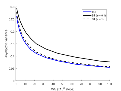
Figure 1: Asymptotic variance of $V(\bm{x})$ as in (30) ($D=1$, thus a double well potential) for simulated tempering algorithms at different switching frequency and the infinite switching limit.

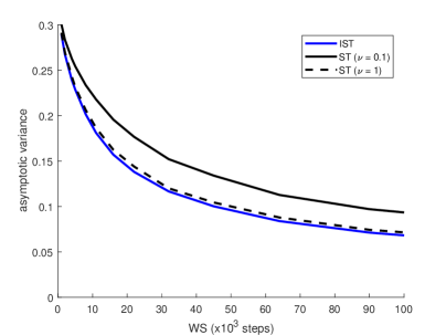
Figure 2: Asymptotic variance of $V(\bm{x})$ as in (30) ($D=10$) for simulated tempering algorithms at different switching frequency and the infinite switching limit.

VII.2 Dimer in solvent example

Now, to test the performance of our algorithm on a more realistic example, we apply (28) for a dimer in solvent model as considered in Dellago et al. (1999). This system consists of $N$ two-dimensional particles in a periodic box with side length $l$. All particles have the same mass $m$, and they interact with each other with the Weeks-Chandler-Anderson potential defined as

$$V_{\text{WCA}}(r)=4\epsilon\left((\sigma/r)^{12}-(\sigma/r)^{6}\right)+\epsilon,$$ (33)

if $r\leq r_{\text{WCA}}=2^{1/6}\sigma$, and $V_{\text{WCA}}(r)=0$ otherwise, except for a pair of particles which interact via a double well potential

$$V_{dW}(r)=h\left(1-\dfrac{(r-r_{\text{WCA}}-\omega)^{2}}{\omega^{2}}\right)^{2}.$$ (34)

We take $N=16$, $l=4.4$, $\sigma=1$, $h=1$, $\omega=0.5$, and $\epsilon=1$ in the simulation. The physical temperature is $T_{0}=0.2$, and one artificial temperatures $T_{1}=1.0$. The total simulation time is set to be $T_{tot}=1.0\times 10^{5}$ with time step $dt=0.001$, which means the total number of steps is $N_{tot}=10^{8}$. The quantity of interest is the free energy associated with the distance of the pair of particles interacting via the double well potential.

In this numerical example, we would still choose the weighting parameter to be inverse partition function, which is however not explicitly known or easily obtained a priori in this case. Therefore, we use the following method to get approximation of these partition functions, similar to that of Gao (2008), and then use the estimates in the weighting factors $n_{k}$. First, a set of initial guess $Z_{k}^{(0)}$ is chosen and used to run the dynamics simulation. Then from a relatively short trajectory, we can add up the corresponding weight to get the ‘proportion’ of each temperature by normalizing their summation to one. Since this proportion would go to $1/2$ if the guess is accurate and the trajectory is infinitely long, we can adjust our guess accordingly. More specifically, if the proportions are $w_{k},\ k=0,1$, the weighting factor will be updated as

$$Z_{k}^{\text{new}}=\begin{cases}Z_{k}^{\text{old}}\times 2w_{k},&\text{if }2w_{k}\in I;\\ Z_{k}^{\text{old}}\times\sqrt{2w_{k}},&\text{otherwise.}\end{cases}$$ (35)

where $I$ is a small neighborhood around $1$ to take into account of the fluctuation due to the short simulation trajectory when estimating $w_{k}$. We iteratively update the partition function estimate $\{Z_{k}^{(l)}\},\,l=1,2,\cdots$ until the proportions $w_{k}$ are satisfactorily close to $1/2$. Here we take $I=[0.35,1.5]$, initial guess $(Z_{0}^{(0)},Z_{1}^{(0)})=(1,10^{8})$ and number of iterations $l_{\max}=10$ with trajectory length $10^{7}$ steps each.

The performance of STMD with various switching rate is shown Fig. 3. It can be seen that the performance of STMD is better when switching rate increases from $0.25$ to $25$; and the asymptotic variance converges to that of the IST as $\nu\to\infty$. This provides strong numerical validation of our theoretical results.

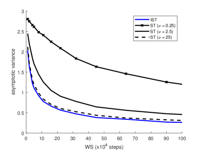
Figure 3: Asymptotic variance of the potential energy $V(\bm{x})$ for the WCA example for simulated tempering algorithms at different switching frequency and the infinite switching limit.

VIII Conclusion

We justify that the sampling efficiency of the simulated tempering method increases with the switching rate of the temperature, using both the theoretical analysis based on large deviation of empirical distribution and also numerical tests on two examples. This motivates taking the infinite switching limit of the simulated tempering dynamics, which recovers the integrated tempering enhanced sampling method under a natural reformulation. The limiting dynamics can be implemented as a patch to standard molecular dynamics by adding a scaling factor to the force term based on a weighted average of all temperatures involved. This leads to a practical scheme with higher sampling efficiency than standard simulated tempering.

Appendix A Derivation of the large deviation rate functional $I^{\nu}(\mu)$

To introduce formally the large deviation principle, let us introduce some definitions. Let $S$ be a Polish space and $\mathcal{P}(S)$ the space of probability measures on $S$, equiped with the topology of weak convergence. Under this weak topology, $\mathcal{P}(S)$ itself is a Polish space. Note that the empirical measure $\lambda_{T}^{\nu}$ is a $\mathcal{P}(S)$-valued random variable.

The large deviation principle for empirical distribution can be stated as follows Donsker and Varadhan (1975); Deuschel and Stroock (1989); Dembo and Zeitouni (2010): A sequence of random probability measures $\{\gamma_{T}\}$ is said to satisfy a large deviation principle with rate function $I:\mathcal{P}(S)\to[0,\infty]$, if for all open sets $O\subset\mathcal{P}(S)$

$$\liminf_{T\to\infty}\frac{1}{T}\log\mathbb{P}(\gamma_{T}\in O)\geq-\inf_{\mu\in O}I(\mu),$$ (36)

for all closed sets $C\subset\mathcal{P}(S)$

$$\liminf_{T\to\infty}\frac{1}{T}\log\mathbb{P}(\gamma_{T}\in C)\leq-\inf_{\mu\in C}I(\mu),$$ (37)

and for all $M<\infty$, $\{\mu:I(\mu)\leq M\}$ is compact in $\mathcal{P}(S)$. In particular, once we obtain the rate functional, (36) and (37) quantifies how unlikely the empirical distribution is far from the equilibrium when $T$ is large, which was used in this work to justify the infinite switching limit.

To find the rate functional $I^{\nu}$ for the simulate tempering overdamped dynamics with switching rate $\nu$, we divide the infinitesimal generator into two parts

$$(\mathcal{L}^{\nu}u)(\bm{x},\beta)=(\mathcal{L}^{\nu}_{\mathrm{diff}}u+\nu\mathcal{L}^{\nu}_{\mathrm{jump}}u)(\bm{x},\beta)\\$$ (38)

where

$$\begin{cases}\mathcal{L}^{\nu}_{\mathrm{diff}}=-\nabla_{\bm{x}}V(\bm{x})\cdot\nabla_{\bm{x}}+\beta^{-1}\nabla_{\bm{x}}\cdot\nabla_{\bm{x}},\\ \mathcal{L}^{\nu}_{\mathrm{jump}}=-g_{\beta,\beta^{\prime}}(\bm{x})+g_{\beta^{\prime},\beta}(\bm{x}).\end{cases}$$ (39)

The rate functional thus has an additive structure (15) with the rate functional $J_{0}$ and $J_{1}$ correspond to $\mathcal{L}^{\nu}_{\mathrm{diff}}$ and $\mathcal{L}^{\nu}_{\mathrm{jump}}$, respectively.

To get an explicit formula of the rate functionals, we first consider $J_{0}$. Let $f(\bm{x},\beta)=\sqrt{\theta(\bm{x},\beta)}$, then following Donsker and Varadan Donsker and Varadhan (1975), we have

$$J_{0}(\mu) =\sum_{\beta}\int f(\mathcal{L}_{\mathrm{diff}}^{\nu}f)\,\varrho(\,\mathrm{d}\bm{x},\beta)$$ (40)

$$= -\sum_{\beta}\int\biggl{[}-(\nabla_{\bm{x}}V(\bm{x})\cdot\nabla_{\bm{x}}f)f$$

$$\qquad\qquad\qquad+(\beta^{-1}\nabla_{\bm{x}}\cdot\nabla_{\bm{x}}f)f\biggr{]}\varrho(\,\mathrm{d}\bm{x},\beta)$$

$$= -\sum_{\beta}\frac{1}{2}Z_{\beta}^{-1}\left\{\int-(\nabla_{\bm{x}}V(\bm{x})\cdot\nabla_{\bm{x}}f)fe^{-\beta V(\bm{x})}\,\mathrm{d}\bm{x}\right.$$

$$\qquad\qquad\qquad+\left.\beta^{-1}\int(\nabla_{\bm{x}}\cdot\nabla_{\bm{x}}f)fe^{-\beta V(\bm{x})}\,\mathrm{d}\bm{x}\right\}$$

$$= -\sum_{\beta}\frac{1}{2}Z_{\beta}^{-1}\left\{\int-(\nabla_{\bm{x}}V(\bm{x})\cdot\nabla_{\bm{x}}f)fe^{-\beta V(\bm{x})}\,\mathrm{d}\bm{x}\right.$$

$$\qquad\qquad\qquad-\left.\beta^{-1}\int\nabla_{\bm{x}}f\cdot\nabla_{\bm{x}}(fe^{-\beta V(\bm{x})})\,\mathrm{d}\bm{x}\right\}$$

$$= -\sum_{\beta}\frac{1}{2}Z_{\beta}^{-1}\left\{-\beta^{-1}\int\lvert\nabla_{\bm{x}}f\rvert^{2}e^{-\beta V(\bm{x})}\,\mathrm{d}\bm{x}\right\}$$

$$= \sum_{\beta}\int\frac{1}{2}\beta^{-1}\lvert\nabla_{\bm{x}}\sqrt{\theta(\bm{x},\beta)}\rvert^{2}\rho_{\beta}(\,\mathrm{d}\bm{x})$$

$$= \sum_{\beta}\int\dfrac{1}{8\theta(\bm{x},\beta)}\left[\beta^{-1}|\nabla_{x}\theta(\bm{x},\beta)|^{2}\right]\rho_{\beta}(\,\mathrm{d}\bm{x}).$$

Next we consider the rate functional $J_{1}$ corresponding to the jump process of the temperature with generator $\mathcal{L}_{\mathrm{jump}}^{\nu}$. From the definition of $\theta(\bm{x},\beta)$, we have

$$\theta(\bm{x},\beta)=\dfrac{2\mu(\bm{x},\beta)}{\rho_{\beta}(\bm{x})},$$ (41)

and therefore

$$\dfrac{\mu(\bm{x},\beta^{\prime})}{\mu(\bm{x},\beta)} =\dfrac{\theta(\bm{x},\beta^{\prime})}{\theta(\bm{x},\beta)}\cdot\dfrac{\rho_{\beta^{\prime}}(\bm{x})}{\rho_{\beta}(\bm{x})}$$ (42)

$$=\dfrac{\theta(\bm{x},\beta^{\prime})}{\theta(\bm{x},\beta)}\cdot\dfrac{g_{\beta,\beta^{\prime}}(\bm{x})}{g_{\beta^{\prime},\beta}(\bm{x})}.$$

Combined with the Cauchy-Schwartz inequality, we obtain that for any choice of non-negative $u(\bm{x},\beta)$

$$\int\bigg{(}g_{\beta^{\prime},\beta}(\bm{x})\dfrac{u(\bm{x},\beta^{\prime})}{u(\bm{x},\beta)}\mu(\,\mathrm{d}\bm{x},\beta)$$ (43)

$$\qquad+g_{\beta,\beta^{\prime}}(\bm{x})\dfrac{u(\bm{x},\beta)}{u(\bm{x},\beta^{\prime})}\mu(\,\mathrm{d}\bm{x},\beta^{\prime})\bigg{)}$$

$$\geq\int 2\sqrt{g_{\beta^{\prime},\beta}(\bm{x})g_{\beta,\beta^{\prime}}(\bm{x})\dfrac{\mu(\bm{x},\beta^{\prime})}{\mu(\bm{x},\beta)}}\mu(\,\mathrm{d}\bm{x},\beta)$$

$$=\int 2g_{\beta,\beta^{\prime}}(\bm{x})\sqrt{\dfrac{\theta(\bm{x},\beta^{\prime})}{\theta(\bm{x},\beta)}}\mu(\,\mathrm{d}\bm{x},\beta),$$

where the equality is attained if and only if for each $\bm{x}\in\mathbb{R}^{3n}$ and each $\beta$ it holds

$$\dfrac{u(\bm{x},\beta^{\prime})}{u(\bm{x},\beta^{\prime})}\propto\dfrac{g_{\beta,\beta^{\prime}}(\bm{x})\mu(\bm{x},\beta^{\prime})}{g_{\beta^{\prime},\beta}(\bm{x})\mu(\bm{x},\beta)}=\dfrac{\rho_{\beta^{\prime}}(\bm{x})\mu(\bm{x},\beta^{\prime})}{\rho_{\beta}(\bm{x})\mu(\bm{x},\beta)}.$$ (44)

In particular, this gives the choice of $u(\bm{x},\beta)$ to make equality holds in (43).

Using the variational characterization of the large deviation rate functional as in Donsker and Varadhan (1975), we have

$$J_{1}(\mu) =-\inf_{u\geq 0}\sum_{\beta}\int\left(\dfrac{\mathcal{L}^{\nu}_{\mathrm{jump}}u}{u}\right)(\bm{x},\beta)\,\mu(\,\mathrm{d}\bm{x},\beta)$$ (45)

$$= -\inf_{u\geq 0}\sum_{\beta}\int\biggl{[}-g_{\beta,\beta^{\prime}}(\bm{x})$$

$$\qquad\qquad\qquad+g_{\beta^{\prime},\beta}(\bm{x})\dfrac{u(\bm{x},\beta^{\prime})}{u(\bm{x},\beta)}\biggr{]}\mu(\,\mathrm{d}\bm{x},\beta)$$

$$= \frac{1}{2}\sum_{\beta}\int\left[g_{\beta,\beta^{\prime}}(x)\mu(\,\mathrm{d}\bm{x},\beta)+g_{\beta^{\prime},\beta}(\bm{x})\mu(\,\mathrm{d}\bm{x},\beta^{\prime})\right]$$

$$-\frac{1}{2}\inf_{u\geq 0}\sum_{\beta}\int\bigg{[}g_{\beta^{\prime},\beta}(\bm{x})\dfrac{u(\bm{x},\beta^{\prime})}{u(\bm{x},\beta)}\mu(\,\mathrm{d}\bm{x},\beta)$$

$$\qquad\qquad+g_{\beta,\beta^{\prime}}(\bm{x})\dfrac{u(\bm{x},\beta)}{u(\bm{x},\beta^{\prime})}\mu(\,\mathrm{d}\bm{x},\beta^{\prime})\bigg{]}$$

$$\overset{\eqref{eq:lemma1J1}}{=} \frac{1}{2}\sum_{\beta}\int g_{\beta,\beta^{\prime}}(x)\left[1+\dfrac{\theta(\bm{x},\beta^{\prime})}{\theta(\bm{x},\beta)}\right]\mu(\,\mathrm{d}\bm{x},\beta)$$

$$-\frac{1}{2}\sum_{\beta}\int 2g_{\beta,\beta^{\prime}}(\bm{x})\sqrt{\dfrac{\theta(\bm{x},\beta^{\prime})}{\theta(\bm{x},\beta)}}\mu(\,\mathrm{d}\bm{x},\beta)$$

$$= \frac{1}{2}\sum_{\beta}\int g_{\beta\beta^{\prime}}(\bm{x})\left[1-\sqrt{\dfrac{\theta(\bm{x},\beta^{\prime})}{\theta(\bm{x},\beta)}}\right]^{2}\mu(\,\mathrm{d}\bm{x},\beta).$$

Therefore, we arrive at the explicit formula for the large deviation rate functionals. We remark that a rigorous proof of the rate functional derived from the above calculation can be found in Dupuis and Liu (2015).

References

- Marinari and Parisi (1992) E. Marinari and G. Parisi, EPL (Europhysics Letters) 19, 451 (1992).
- Kerler and Rehberg (1994) W. Kerler and P. Rehberg, Physical Review E 50, 4220 (1994).
- Hansmann (1997) U. H. Hansmann, Chemical Physics Letters 281, 140 (1997).
- Sugita and Okamoto (1999) Y. Sugita and Y. Okamoto, Chemical physics letters 314, 141 (1999).
- Earl and Deem (2005) D. J. Earl and M. W. Deem, Physical Chemistry Chemical Physics 7, 3910 (2005).
- Zhang and Ma (2008) C. Zhang and J. Ma, The Journal of chemical physics 129, 134112 (2008).
- Gao (2008) Y. Q. Gao, The Journal of chemical physics 128, 064105 (2008).
- Yang et al. (2009) L. Yang, Q. Shao, and Y. Q. Gao, J. Chem. Phys. 130, 124111 (2009).
- Yang et al. (2015) L. Yang, C. W. Liu, Q. Shao, J. Zhang, and Y. Q. Gao, Acc. Chem. Res. 48, 947 (2015).
- Dellago et al. (1999) C. Dellago, P. G. Bolhuis, and D. Chandler, The Journal of chemical physics 110, 6617 (1999).
- Sindhikara et al. (2008) D. Sindhikara, Y. Meng, and A. E. Roitberg, The Journal of chemical physics 128, 01B609 (2008).
- Plattner et al. (2011) N. Plattner, J. D. Doll, P. Dupuis, H. Wang, Y. Liu, and J. E. Gubernatis, J. Chem. Phys. 135, 134111 (2011).
- Dupuis et al. (2012) P. Dupuis, Y. Liu, N. Plattner, and J. D. Doll, Multiscale Modeling & Simulation 10, 986 (2012).
- Lu and Vanden-Eijnden (2013) J. Lu and E. Vanden-Eijnden, The Journal of chemical physics 138, 084105 (2013).
- Yu et al. (2016) T.-Q. Yu, J. Lu, C. F. Abrams, and E. Vanden-Eijnden, Proceedings of the National Academy of Sciences (2016).
- Lu and Vanden-Eijnden (2017) J. Lu and E. Vanden-Eijnden, “Methodological and computational aspects of parallel tempering methods in the infinite swapping limit,” (2017), preprint arXiv:1712.06947.
- (17) A. Martinsson, J. Lu, B. Leimkuhler, and E. Vanden-Eijnden, In preparation.
- Park and Pande (2007) S. Park and V. S. Pande, Phys. Rev. B 76, 016703 (2007).
- Tan (2017) Z. Tan, J. Comput. Graph. Stat. 26, 54 (2017).
- Donsker and Varadhan (1975) M. D. Donsker and S. Varadhan, Comm. Pure Appl. Math. 28, 1 (1975).
- Deuschel and Stroock (1989) J. D. Deuschel and D. W. Stroock, Large deviation, Pure and Applied Mathematics, Vol. 137 (Academic Press, New York, 1989).
- Dembo and Zeitouni (2010) A. Dembo and O. Zeitouni, Large Deviation Techniques and Applications (Springer, 2010).
- Dupuis and Liu (2015) P. Dupuis and Y. Liu, Ann. Probab. 43, 1121 (2015).