Mass Modeling of Frontier Fields Cluster MACS J1149.5+2223
Using Strong and Weak Lensing

Abstract

We present a gravitational lensing model of MACS J1149.5+2223 using ultra-deep Hubble Frontier Fields imaging data and spectroscopic redshifts from HST grism and VLT/MUSE spectroscopic data. We create total mass maps using 38 multiple images (13 sources) and 608 weak lensing galaxies, as well as 100 multiple images of 31 star-forming regions in the galaxy that hosts Supernova Refsdal. We find good agreement with a range of recent models within the HST field of view. We present a map of the ratio of projected stellar mass to total mass ($f_{\star}$), and find that the stellar mass fraction for this cluster peaks on the primary BCG. Averaging within a radius of 0.3 Mpc, we obtain a value of $\langle f_{\star}\rangle=0.012^{+0.004}_{-0.003}$, consistent with other recent results for this ratio in cluster environments, though with a large global error (up to $\delta f_{\star}=0.005$) primarily due to the choice of an IMF. We compare values of $f_{\star}$ and measures of star formation efficiency for this cluster to other Hubble Frontier Fields clusters studied in the literature, finding that MACS1149 has a higher stellar mass fraction than these other clusters, but a star formation efficiency typical of massive clusters.

1. Introduction

Galaxy cluster mass models are among the most useful applications of the theory of gravitational lensing to early-universe cosmology. Especially at redshifts near $z\sim 0.5$, massive galaxy clusters have wide areas of large magnification power, and thus have significant implications for observing faint, high-redshift background objects (Bradač et al., 2014; Mohammed et al., 2016, and references therein). Magnification modeling is needed to constrain the faint end of the $z=6-8$ rest-frame UV (Ishigaki et al., 2017; Livermore et al., 2017; Bouwens et al., 2016; Robertson et al., 2015, and references therein) luminosity functions. At lower redshifts ($z=0.7-2.3$), galaxy evolution studies have used gravitational lensing to spatially resolve galaxy kinematic properties and chemical abundances (Mason et al., 2016; Wang et al., 2015; Vulcani et al., 2016; Leethochawalit et al., 2016; Jones et al., 2015; Christensen et al., 2012; Richard et al., 2011; Jones et al., 2010; Stark et al., 2008, and references therein).

Recent analyses have determined that, in extreme cases, differences in magnification models can be responsible for systematic uncertainties up to several orders of magnitude for lensed sources as faint as $-12$ mag (Bouwens et al., 2016). Uncertainties in magnification have significant implications on estimates of the faint end of the luminosity function (Bouwens et al., 2016), underlining the necessity of producing magnification maps using a variety of independent techniques to quantify the effects of model systematics (Priewe et al., 2017). The majority of cluster magnification maps use parametric modeling techniques (i.e, techniques that assume an underlying relationship between dark and luminous matter), which typically share the same class of systematic biases. Thus, it is critical to produce additional magnification maps using free-form techniques (Mohammed et al., 2016).

In addition to their value in producing magnification maps, galaxy cluster mass models yield insight into a number of dark matter properties, including the key assumption that light traces mass (LTM). The role of dark matter in cluster physics is still poorly understood, and is thus a large source of systematic error in simulations of cluster physics (Dubois et al., 2013; Laporte & White, 2015; Martizzi et al., 2014; Mohammed et al., 2016). Current theoretical models underpinning cluster simulation studies, such as the cluster subhalo mass function (Natarajan et al., 2017; Mohammed et al., 2016; Atek et al., 2015, and references therein), depend on the validity of the assumption of LTM. Without testing this claim, it is also impossible to investigate alternative theories that challenge $\Lambda$CDM, such as dark matter self-interaction (Markevitch et al., 2004; Clowe et al., 2006). Thus, mass models that avoid LTM assumptions are critical for improving the theoretical models underlying cluster simulations.

Additionally, the distribution of cluster baryonic matter can reveal whether cluster baryons are representative of universal baryonic material (e.g., Gonzalez et al., 2013; Nagai et al., 2007; Simionescu et al., 2011, and references therein), and may provide explanation for how efficiently stellar material is formed in clusters by comparing the stellar material in clusters to the cluster gas mass (Gonzalez et al., 2013; Behroozi et al., 2013; Kravtsov et al., 2014, among others) and total baryon fraction (Gonzalez et al., 2013; Lin et al., 2003; Budzynski et al., 2014). Investigations of star formation efficiency have implications for simulations of galaxy evolution (Gonzalez et al., 2013, and references therein) in cluster contexts, particularly of the role of radiative cooling and/or stellar feedback in heating the ICM and altering its metallicity (Dolag et al., 2009; Ettori et al., 2006; Kravtsov et al., 2005; De Lucia et al., 2004; Valdarnini, 2003).

One way to address these questions of cluster composition is to compare the distribution of the ratio of stellar mass to total mass within galaxy clusters. (Bahcall et al., 1995; Bahcall & Kulier, 2014, and references therein). Several authors have calculated this ratio for many clusters and over a range of distance scales (e.g. Bahcall & Kulier, 2014; Gonzalez et al., 2013; Wang et al., 2015; Hoag et al., 2016; Jauzac et al., 2012, 2016). Bahcall & Kulier (2014) have found that on scales larger than a few kpc, the ratio of stellar mass to total mass is roughly constant, suggesting that stellar mass traces total mass when averaged over large apertures. Galaxy cluster mass models are critical to producing these results (Mohammed et al., 2016; Wang et al., 2015; Hoag et al., 2016).

The galaxy cluster MACS1149.5+2223 ($z=0.544$, MACS1149 hereafter) has been extensively studied due to its complex merging properties and potential as a lensing cluster. It was first identified as part of the MAssive Cluster Survey (MACS: Ebeling et al., 2001), and has been subsequently observed in the optical band by the Cluster Lensing And Supernova survey with Hubble (CLASH: Postman et al., 2012) and the Hubble Frontier Fields initiative (HFF: Lotz et al., 2016; Coe et al., 2015), as well as by observations in other wavelengths. As a result, the mass distribution of MACS1149 has been modelled with a variety of lens-modeling techniques (Smith et al., 2009; Zitrin & Broadhurst, 2009; Zitrin et al., 2011; Richard et al., 2014; Coe et al., 2015; Johnson et al., 2014; Rau et al., 2014; Mohammed et al., 2016), which give broadly similar cluster mass distributions.

The discovery of Supernova Refsdal ($z_{s}=1.49$, Kelly et al., 2015, 2016) in the center of MACS1149 is of particular interest to the modeling community, as it demonstrated the possibility of using clusters as lenses to magnify multiply-imaged background supernovae. While lensed supernovae had previously been predicted (Refsdal, 1964) and observed (Rodney et al., 2015a), the time delay between SN Refsdal’s multiple images provided a valuable opportunity to test the accuracy of mass models (Treu et al., 2016; Johnson & Sharon, 2016; Jauzac et al., 2016; Diego et al., 2016; Grillo et al., 2016) in the center of the cluster, and the predicted magnifications of these images can be compared to observed flux ratios to provide a tight constraint on the model near the BCG.

In this paper, we present a strong and weak gravitational lensing model of MACS1149 using HFF data by modeling the cluster with our Strong and Weak Lensing United (SWUnited) method (Bradač et al., 2009, 2005). Unlike the majority of lens modeling methods previously used to study MACS1149, SWUnited does not explicitly fit the parameters of an underlying dark matter distribution that traces stellar light. Indeed, this is the only mass map of MACS1149 to date that is produced with both HFF data and a non-parametric (gridded) modeling approach. We compare our results to recent models of strongly lensed systems in MACS1149 presented by Johnson & Sharon (2016); Diego et al. (2016); Grillo et al. (2016); Jauzac et al. (2016); Oguri (2015); Kawamata et al. (2016); Treu et al. (2016).

We also present a map of the stellar mass to total mass ratio, the first of its kind to be produced for MACS1149. Since MACS1149 is a massive and dynamically complex cluster, it is interesting to consider how well its stellar material traces its dark matter. We discuss the distribution of this value across the cluster, and its implications for estimates of star formation efficiency.

The paper proceeds as follows: in section 2, we describe in detail the data used for spectroscopic and photometric redshift identification, as well as for weak lensing. Section 3 discusses the process of modeling MACS1149 using the SWUnited method and presents modeling results; a stellar mass to total mass ratio map is presented in section 4. Finally, section 5 concludes these results.

Throughout the paper, we adopt a cosmology with $\Omega_{m}=0.3$, $\Omega_{\Lambda}=0.7$, and $h=0.7$. We give all magnitudes in the AB system (Oke, 1974).

2. Data and Image Identification

To constrain our mass model, we use imaging data to identify strongly-lensed multiple images and weakly-lensed background galaxies, and to estimate their redshifts. We use spectroscopic data to more accurately estimate multiple image redshifts (Treu et al., 2015), since lens models tend to substantially improve with more spectroscopic data (Rodney et al., 2015a, b).

2.1. HST and VLT Spectroscopic Data

Original spectroscopy for MACS1149 was obtained from the Grism Lens-Amplified Survey from Space (GLASS: Schmidt, 2014; Treu et al., 2015)^,, which was initiated to study highly-magnified high-redshift objects. The GLASS collaboration obtained 14 HST orbits per cluster, with the WFC3-IR G102 (10 orbits) and G141 (4 orbits) grisms (field of view $123\times 136\farcs$). Each observation was taken at two position angles $90^{\circ}\pm 10^{\circ}$ apart to improve deblending and spectrum extraction. The extraction apertures were $0\farcs 6\times 100\AA$ (5 spatial by 3 spectral native pixels). The average spectral resolution was $R\sim 130$ for the G141 grism, and $R\sim 210$ for the G102 grism. Overall, the spectra covered a continuous wavelength range of $0.81-1.69\mu$m. Direct image exposures were taken in the F105W and F140W bands to ensure image alignment and calibration (Treu et al., 2015). Deep HST G141 data were taken as part of the Supernova Refsdal follow-up campaign (HST-GO-14041; PI Kelly Kelly et al., 2016), adding another 30 orbits of G141 spectra.

In addition to the HST spectroscopy, spectroscopic data were taken with VLT/Multi Unit Spectroscopic Explorer (MUSE, Bacon et al., 2010); these observations were designed to measure multiple image redshifts and to observe SN Refsdal (Karman et al., 2016; Kelly et al., 2016; Grillo et al., 2016; Rodney et al., 2015a). Observations were taken in the wavelength range $480-930$ nm, with a total integration time of 4.8 hours. The field of view was $1\times 1\farcm$, with an average spectral resolution of $R\sim 3000$. Most spectroscopic redshifts of multiply-imaged objects in this work were obtained from the VLT/MUSE data due to its sensitivity and wavelength coverage being more favorable than those of GLASS for the sources in question. Further details of these observations and analyses are discussed in Grillo et al. (2016); Kelly et al. (2016).

2.2. HST and Spitzer Imaging Data

As part of the HFF initiative (HST-GO 13504, PI J. Lotz), MACS1149 was observed in seven filters: three ACS/optical filters (F435W, F606W, F814W) and four WFC3/IR filters (F105W, F125W, F140W, F160W). These data were taken between November 2014 and June 2015 (141 orbits), and were supplemented by additional WFC3/NIR data from the SN Refsdal follow-up campaign (20 orbits, PI Rodney HST-GO 13790, PI Kelly HST-GO 14041). We use both epochs of the public release data products from the HFF team, yielding a $5\sigma$ point source sensitivity of $\sim 29$mag per band. Further supplementary data were obtained from the CLASH program (20 orbits, Postman et al., 2012), and were primarily used to construct our photometric catalog.

We use deep Spitzer/Infrared Array Camera (IRAC) images in combination with the HST images to improve stellar mass and photometric redshift measurements of cluster members and background galaxies. The final Spitzer/IRAC imaging mosaic, made available by P. Capak, includes data taken by the IRAC Lensing Survey (PI: Egami), Spitzer UltRa Faint SUrvey Program (SURFSUP: Bradač et al., 2014; Ryan et al., 2014; Huang et al., 2016), and the Spitzer Frontier Fields program (Capak et al., in prep). The mosaic is comprised of ten dithered $5\farcm 2\times 5\farcm 2$ images, with a total field of view of $20\farcm 6\times 29\farcm 6$ ($7.9\times 11.3$ Mpc). The combined exposure time reaches $\sim$50 hours in each of channel 1 ($3.6\mu$m) and channel 2 ($4.5\mu$m). The images reach a $5\sigma$ limiting magnitude of $\sim$26.5 mag (channel 1) and $\sim$26.0 (channel 2) for a point source outside the cluster core, sensitive enough to probe the bulk of cluster member stellar mass.

2.3. Photometry

The majority of the background sources do not have spectroscopic redshifts, so their redshifts are estimated using photometric measurements from HST images. We follow the procedure by Huang et al. (2016) to measure broadband flux densities. In short, we first convolve all images blueward of F160W with PSF smoothing kernels to match the PSF width in F160W. We do this by using the psfmatch task in IRAF to compute the PSF kernels on individual point sources in the cluster field. We measured the FWHM of the PSF in F160W and found that it is around $0\farcs 18-0\farcs 2$. We also compared the curves of growth using point sources across different filters and found that after convolving with PSF-matching kernels, the curves of growth generally agree with that in F160W to within $15\%$. We then measure broadband flux densities using SExtractor (Bertin & Arnouts, 1996) in dual-image mode, with the F160W image as the detection image. The total flux density of each source is measured within an elliptical Kron aperture with $k=2.5$ (Kron, 1980, called MAG_AUTO in SExtractor), and the colors are calculated using the flux densities measured within isophotal apertures (called MAG_ISO in SExtractor).

Photometric redshift of each source is estimated using the colors in HST and Spitzer filters. We use the photometric redshift code EAZY (Brammer et al., 2008) which employs a template-fitting approach using a set of templates that are optimized for redshift estimation. The code produces probability distribution functions for the redshifts of each source; we take the peak of this distribution as our photometric redshift estimate and use the distribution to derive our confidence intervals. In our redshift fitting process, we do not employ a redshift prior, and a comparison with known spectroscopic redshifts shows that the photometric redshifts are consistent with spectroscopic redshifts within error bars.

2.4. Weak Lensing Catalog

We generate a weak lensing catalog based on a 26.9ks deep stack of ACS F606W imaging using the pipeline described in Schrabback et al. (2018a). This pipeline utilizes the Erben et al. (2001) implementation of the KSB+ algorithm (Kaiser et al., 1995b; Luppino & Kaiser, 1997; Hoekstra et al., 1998) for galaxy shape measurements as detailed in Schrabback et al. (2007). It additionally employs the pixel-level correction for charge-transfer inefficiency from Massey et al. (2014), as well as a correction for noise-related shape measurement biases and a principal component model for the temporally and spatially varying ACS point-spread function (Schrabback et al., 2010). Schrabback et al. (2018b) and Hernández-Martín et al. (in prep) have extended earlier simulation-based tests of the employed shape measurement pipeline to the non-weak shear regime of clusters (for $|g|\leq 0.4$), confirming that residual multiplicative shear estimation biases are small ($|m|\lesssim 5\%$). For the source selection and redshift estimation we follow Hoag et al. (2016), cross-matching objects in our weak lensing catalog with those in our photometric catalog produced from CLASH data.

2.5. Strong Lensing Catalog

We use strong lensing images to constrain our mass model. In this work, we use the grading system of the Treu et al. (2016) modeling collaboration (Wang et al., 2015; Hoag et al., 2016; Treu et al., 2016), identifying multiple images as being part of the same system using color, morphology, and spectral emission features. Each potential multiple image system was inspected by five independent teams of the HFF collaboration and identified as gold (very likely to be images from the same system) or silver (likely to be images from the same system) based on image colors and morphologies. Any systems not classified as gold or silver are not likely to be multiple images, and they are not used in this model.

A total of 23 images (8 systems) are spectroscopically confirmed by Treu et al. (2016), and are listed in Table 1. In system 13, the images have somewhat different spectroscopic redshifts despite being consistent morphologically with each other. The spectra were obtained from HST grism observations with a $68\%$ confidence interval of $\pm 50\AA$, which corresponds to a $\delta_{z}\approx 0.01$. One image has a spectroscopic redshift of $z=1.25\pm 0.01$ and the other two have redshifts of $z=1.23\pm 0.01$, so for this system the average of the individual spectroscopic redshifts was used as the system redshift. Because of the strong morphological consistency and correct parity of the system, it is considered to be a true system. A second system (system 5) had only one of its images spectroscopically confirmed; the other images are considered to share the same redshift based on their colors and morphologies.

We supplement the spectroscopically-confirmed multiple images with 15 images (5 systems) identified photometrically as strong multiple image candidates. An example of a photometric redshift P($z$) for a strongly-lensed system is shown in Figure 1. For multiple images not confirmed by spectroscopy, the model presented in this work includes only systems with at least two images that have coinciding peaks (i.e., peaks are within each other’s 68% confidence intervals) in redshift probability density functions, P($z$), and whose most likely photometric redshifts are greater than the cluster redshift. Redshift estimates used in the mass model are listed in Table 1. Some of the multiple images are blended with foreground sources; thus, their redshifts cannot be reliably estimated and we remove their incorrect P($z$) from our strong lensing redshift estimates.

In addition to using these multiple images of sources in independent redshift planes, we further constrain the model using 100 images of 31 unique star-forming regions present in the highly-resolved spiral galaxy that hosts SN Refsdal (Table 2, Treu et al., 2016). Several images of this galaxy appear near the cluster center, and the number and quality of these associated multiple images provides a powerful constraint to the mass model in these central regions. All of the images of the star-forming regions in the SN Refsdal host galaxy were included in several models (Diego et al., 2016; Kawamata et al., 2016; Sharon & Johnson, 2015; Grillo et al., 2016), and most were included by Grillo et al. (2016), Zitrin et al. (in prep) as well.

Of the 138 images (44 systems) used in the model, 123 images (39 systems) have spectroscopically measured redshift and only 15 images (5 systems) are identified photometrically, so we are confident in the robustness of our strong lensing catalog.

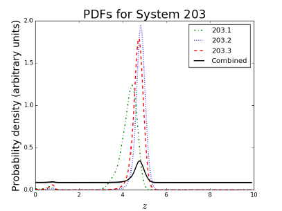
Figure 1.— Example of a normalized redshift probability density function, P($z$) for multiple images in a photometric system. The bold black line shows combined redshift probability density functions for multiple images in photometric systems, as obtained by our Bayesian combination procedure.

Table 1Multiply Imaged Systems

ID	$\alpha$	$\delta$	Spec-$z$	Peak	System	Magnification	Category
	(J2000)	(J2000)		P($z$)	Redshift
1.1	177.39700	22.39600	1.488	$\cdots$	1.488	$12\pm 1$	Gold
1.2	177.39942	22.39743	1.488	$\cdots$	$\cdots$	$7.3\pm 0.5$	Gold
1.3	177.40342	22.40243	1.488	$1.5^{+0.1}_{-0.3}$	$\cdots$	$3.90\pm 0.04$	Gold
1.5	177.39986	22.39713	$\cdots$	$\cdots$	$\cdots$	$13\pm 2$	Silver
2.1	177.40242	22.38975	1.891	$2.3^{+0.2}_{-0.1}$	1.891	$4.9_{-0.2}^{+0.1}$	Gold
2.2	177.40604	22.39247	1.891	$\cdots$	$\cdots$	$35_{-1}^{+23}$	Gold
2.3	177.40658	22.39288	1.891	$2.4\pm 0.1$	$\cdots$	$13\pm 2$	Gold
3.1	177.39075	22.39984	3.129	$3.2\pm 0.1$	3.129	$16\pm 1$	Gold
3.2	177.39271	22.40308	3.129	$\cdots$	$\cdots$	$13_{-1}^{+2}$	Gold
3.3	177.40129	22.40718	3.129	$3.4\pm 0.1$	$\cdots$	$6.0\pm 0.1$	Gold
4.1	177.39300	22.39682	2.949	$\cdots$	2.949	$12.5_{-0.4}^{+0.5}$	Gold
4.2	177.39438	22.40073	2.949	$\cdots$	$\cdots$	$8.8\pm 0.2$	Gold
4.3	177.40417	22.40612	2.949	$2.6^{+0.1}_{-0.2}$	$\cdots$	$4.3_{-0.2}^{+0.1}$	Gold
5.1	177.39975	22.39306	2.80	$\cdots$	2.80	$26_{-10}^{+7}$	Gold
5.2	177.40108	22.39382	$\cdots$	$2.6\pm 0.1$	$\cdots$	$9_{-1}^{+6}$	Gold
5.3	177.40792	22.40355	$\cdots$	$2.8\pm 0.1$	$\cdots$	$5.0_{-0.4}^{+1.0}$	Silver
6.1	177.39971	22.39254	$\cdots$	$\cdots$	$2.65_{-1.81}^{+3.75}$	$10_{-4}^{+6}$	Gold
6.2	177.40183	22.39385	$\cdots$	$2.6^{+0.1}_{-2.3}$	$\cdots$	$7.0_{-0.5}^{+1.1}$	Gold
6.3	177.40804	22.40250	$\cdots$	$\cdots$	$\cdots$	$5.5_{-0.1}^{+0.2}$	Silver
7.1	177.39896	22.39133	$\cdots$	$2.6\pm 0.1$	$2.56_{-1.69}^{+3.84}$	$6.3_{-0.8}^{+18.0}$	Gold
7.2	177.40342	22.39426	$\cdots$	$2.7^{+0.1}_{-0.2}$	$\cdots$	$5.2\pm 0.2$	Gold
7.3	177.40758	22.40124	$\cdots$	$2.3^{+0.1}_{-0.2}$	$\cdots$	$4.4_{-0.6}^{+0.2}$	Gold
13.1	177.40371	22.39778	1.23	$1.3\pm 0.1$	1.24	$12.1_{-0.9}^{+0.7}$	Gold
13.2	177.40283	22.39665	1.25	$\cdots$	$\cdots$	$11.5_{-0.3}^{+0.4}$	Gold
13.3	177.40004	22.39385	1.23	$0.8^{+0.2}_{-0.1}$	$\cdots$	$5.1_{-0.5}^{+0.3}$	Gold
14.1	177.39167	22.40348	3.703	$3.4^{+0.2}_{-0.1}$	3.703	$17_{-1}^{+2}$	Gold
14.2	177.39083	22.40264	3.703	$3.4\pm 0.1$	$\cdots$	$43_{-5}^{+7}$	Gold
110.1	177.40014	22.39016	3.214	$3.2^{+0.1}_{-0.2}$	3.214	$6.4_{-1.0}^{+0.3}$	Gold
110.2	177.40402	22.39289	3.214	$\cdots$		$5.4_{-0.5}^{+0.2}$	Gold
26.1	177.41035	22.38874	$\cdots$	$3.3\pm 0.1$	$3.29_{-2.40}^{+3.06}$	$38_{-21}^{+37}$	Silver
26.2	177.40922	22.38769	$\cdots$	$3.1^{+0.1}_{-0.2}$	$\cdots$	$74_{-72}^{+172}$	Silver
26.3	177.40623	22.38536	$\cdots$	$3.4\pm 0.1$	$\cdots$	$5.8_{-0.3}^{+0.4}$	Silver
203.1	177.40995	22.38724	$\cdots$	$4.4^{+0.2}_{-0.5}$	$4.70_{-3.73}^{+1.37}$	$49_{-2}^{+50}$	Silver
203.2	177.40657	22.38451	$\cdots$	$4.8\pm 0.2$	$\cdots$	$5.3_{-0.3}^{+0.2}$	Silver
203.3	177.41123	22.38846	$\cdots$	$4.8^{+0.2}_{-0.3}$	$\cdots$	$15_{-3}^{+5}$	Silver
204.1	177.40961	22.38666	$\cdots$	$6.1^{+2.0}_{-4.1}$	$6.47_{-5.35}^{+0.18}$	$8_{-2}^{+5}$	Silver
204.2	177.40668	22.38432	$\cdots$	$6.2^{+0.2}_{-4.8}$	$\cdots$	$5.5\pm 0.4$	Silver
204.3	177.41208	22.38905	$\cdots$	$6.8\pm 0.3$	$\cdots$	$13\pm 1$	Silver

Note. — All multiple images used in the gravitational mass model, with magnifications produced by the model, excluding the multiple images associated with SN Refsdal and its host galaxy (see 2). System 5 had only one spectroscopically-confirmed image; in the model, the entire system is assumed to be at this redshift. System 13 had two slightly different spectroscopic redshifts; the average of the redshifts was used in the modeling. For original identification references, see Treu et al. (2015). Spectroscopic redshifts are obtained using data obtained from the GLASS program and the Refsdal Follow-up Campaign. Photometric redshifts (Peak P($z$)) are for individual images rather than combined system redshifts. Combined system redshifts for photometric systems are determined by combining the individual P($z$) using a Bayesian combination procedure; the peak value for the resultant combined P($z$) is considered to be the system redshift. In the System Redshift column we have also included effective $1\sigma$ uncertainties for photometric systems. These uncertainties are the lower and upper bound values which yield $34\%$ on each side of the median combined P($z$) when integrating under the P($z$) curve. The uncertainties are much larger than typical photometric redshift uncertainties, given that we account for the possibility of catastrophic errors by combining the individual system P($z$) curves with a uniform PDF.

Table 2Multiple Images of Star-Forming Knots in the SN Refsdal Host Galaxy

ID	$\alpha$ (J2000)	$\delta$ (J2000)	Magnification
1.1.1	177.39702	22.39600	$12\pm 1$
1.1.2	177.39942	22.39743	$7.3\pm 0.5$
1.1.3	177.40341	22.40244	$3.90\pm 0.04$
1.1.5	177.39986	22.39713	$12\pm 2$
1.2.1	177.39661	22.39630	$12.8\pm 0.7$
1.2.2	177.39899	22.39786	$23_{-8}^{+16}$
1.2.3	177.40303	22.40268	$3.96_{-0.04}^{+0.02}$
1.2.4	177.39777	22.39878	$12.0_{-0.6}^{+1.1}$
1.2.6	177.39867	22.39824	$2.8_{-0.2}^{+0.3}$
1.3.1	177.39687	22.39621	$13.1_{-0.9}^{+0.6}$
1.3.2	177.39917	22.39760	$13_{-1}^{+2}$
1.3.3	177.40328	22.40259	$3.89\pm 0.03$
1.4.1	177.39702	22.39621	$13_{-1}^{+2}$
1.4.2	177.39923	22.39748	$12_{-1}^{+2}$
1.4.3	177.40339	22.40255	$3.88\pm 0.04$
1.5.1	177.39726	22.39620	$13\pm 1$
1.5.2	177.39933	22.39730	$12_{-1}^{+2}$
1.5.3	177.40356	22.40252	$3.83_{-0.07}^{+0.04}$
1.6.1	177.39737	22.39616	$15\pm 1$
1.6.2	177.39945	22.39723	$8.8_{-0.7}^{+0.9}$
1.6.3	177.40360	22.40248	$3.83_{-0.07}^{+0.04}$
1.7.1	177.39757	22.39611	$18\pm 2$
1.7.2	177.39974	22.39693	$12\pm 2$
1.7.3	177.40370	22.40240	$3.84_{-0.08}^{+0.04}$
1.8.1	177.39795	22.39601	$27_{-3}^{+5}$
1.8.2	177.39981	22.39675	$9.4\pm 0.5$
1.8.3	177.40380	22.40231	$3.74_{-0.10}^{+0.05}$
1.9.1	177.39803	22.39593	$27_{-3}^{+5}$
1.9.2	177.39973	22.39698	$12\pm 2$
1.9.3	177.40377	22.40225	$3.88_{-0.08}^{+0.06}$
1.10.1	177.39809	22.39585	$46_{-12}^{+18}$
1.10.2	177.39997	22.39670	$6.7_{-0.4}^{+0.5}$
1.10.3	177.40380	22.40218	$3.88_{-0.08}^{+0.06}$
1.11.2	177.40010	22.39666	$4.6_{-0.4}^{+0.5}$
1.11.3	177.40377	22.40204	$3.94_{-0.07}^{+0.04}$
1.12.1	177.39716	22.39521	$7.9_{-0.5}^{+0.6}$
1.12.2	177.40032	22.39692	$6.1_{-0.3}^{+0.4}$
1.12.3	177.40360	22.40187	$4.07_{-0.05}^{+0.04}$
1.13.1	177.39697	22.39663	$17.7_{-1.1}^{+0.8}$
1.13.2	177.39882	22.39771	$67_{-206}^{+140}$
1.13.3	177.40329	22.40282	$3.90_{-0.05}^{+0.03}$
1.13.4	177.39791	22.39843	$22_{-3}^{+7}$
1.14.1	177.39712	22.39672	$20_{-2}^{+1}$
1.14.2	177.39878	22.39763	$27_{-7}^{+12}$
1.14.3	177.40338	22.40287	$3.63_{-0.08}^{+0.02}$
1.14.4	177.39810	22.39825	$48_{-22}^{+114}$
1.15.1	177.39717	22.39650	$20\pm 2$
1.15.2	177.39894	22.39751	$25_{-5}^{+8}$
1.15.3	177.40344	22.40275	$3.81_{-0.05}^{+0.03}$
1.16.1	177.39745	22.39640	$19\pm 2$
1.16.2	177.39915	22.39722	$15\pm 1$
1.16.3	177.40360	22.40265	$3.67_{-0.10}^{+0.02}$
1.17.1	177.39815	22.39634	$26_{-6}^{+7}$
1.17.2	177.39927	22.39683	$22_{-2}^{+3}$
1.17.3	177.40384	22.40256	$3.67_{-0.10}^{+0.04}$
1.18.1	177.39850	22.39610	$105_{-44}^{+102}$
1.18.2	177.39947	22.39659	$14\pm 1$
1.18.3	177.40394	22.40240	$3.68_{-0.12}^{+0.05}$
1.19.1	177.39689	22.39576	$10.2\pm 0.6$
1.19.2	177.39954	22.39748	$5.6_{-0.4}^{+0.3}$
1.19.3	177.40337	22.40229	$4.1\pm 0.2$
1.19.5	177.39997	22.39710	$16_{-7}^{+33}$
1.20.1	177.39708	22.39572	$9.2\pm 0.6$
1.20.2	177.39963	22.39736	$6.2_{-0.4}^{+0.7}$
1.20.3	177.40353	22.40223	$3.92_{-0.08}^{+0.03}$
1.20.5	177.40000	22.39698	$14_{-7}^{+26}$
1.21.1	177.39694	22.39540	$8.0_{-0.7}^{+0.8}$
1.21.3	177.40341	22.40200	$4.12_{-0.02}^{+0.03}$
1.21.5	177.40018	22.39704	$25_{-49}^{+50}$
1.22.1	177.39677	22.39548	$8.6_{-0.8}^{+0.6}$
1.22.2	177.39968	22.39749	$5.6_{-0.4}^{+0.3}$
1.22.3	177.40328	22.40209	$4.17_{-0.04}^{+0.06}$
1.22.5	177.40008	22.39713	$44_{-105}^{+76}$
1.23.1	177.39672	22.39538	$7.8_{-0.5}^{+0.7}$
1.23.2	177.39977	22.39749	$5.3\pm 0.3$
1.23.3	177.40324	22.40201	$4.17_{-0.04}^{+0.06}$
1.23.5	177.40013	22.39720	$44_{-105}^{+76}$
1.24.1	177.39650	22.39558	$8.8_{-0.9}^{+0.6}$
1.24.2	177.39953	22.39775	$6.5_{-0.3}^{+0.7}$
1.24.3	177.40301	22.40220	$4.19_{-0.03}^{+0.04}$
1.25.1	177.39657	22.39593	$10.9_{-0.8}^{+0.7}$
1.25.3	177.40304	22.40245	$4.00\pm 0.03$
1.26.1	177.39633	22.39601	$8.8_{-0.8}^{+0.7}$
1.26.3	177.40283	22.40260	$4.10_{-0.03}^{+0.02}$
1.27.1	177.39831	22.39628	$138_{-478}^{+335}$
1.27.2	177.39933	22.39672	$20\pm 2$
1.28.1	177.39860	22.39616	$104_{-44}^{+102}$
1.28.2	177.39942	22.39655	$18_{-1}^{+2}$
1.29.1	177.39858	22.39586	$19_{-2}^{+3}$
1.29.2	177.39976	22.39649	$12.6_{-0.5}^{+0.7}$
1.30.1	177.39817	22.39546	$30_{-5}^{+13}$
1.30.2	177.39801	22.39523	$24_{-3}^{+4}$
1.30.3	177.39730	22.39536	$8.7_{-1.0}^{+0.7}$
1.30.4	177.39788	22.39572	$41_{-12}^{+17}$
S1	177.39823	22.39563	$30_{-4}^{+6}$
S2	177.39772	22.39578	$22\pm 3$
S3	177.39737	22.39553	$11\pm 1$
S4	177.39781	22.39518	$15\pm 2$
SX	177.40024	22.39681	$6.30_{-0.4}^{+0.5}$
SY	177.4038	22.40214	$3.88_{-0.08}^{+0.06}$

Note. — All star-forming knots in the host galaxy of SN Refsdal ($z_{s}=1.49$), as well as all images of the supernova, with magnifications produced by the model. Objects S1-S4, SX, and SY are images of SN Refsdal; they are also used as model inputs. For original identification references, see Treu et al. (2015). Magnification uncertainties allowing for negative values indicate that crossing the critical curve lies in the 68% confidence interval of magnification values.

3. Mass Modeling

3.1. Summary of the Modeling Procedure

In order to model the mass distribution of MACS1149, we use the Strong and Weak Lensing United (SWUnited) code developed by Bradač et al. (2009, 2005), which has previously been used to model other HFF clusters (Hoag et al., 2016; Wang et al., 2015). This software extends weak lensing reconstruction to critical regions, thus using information from both strongly-lensed multiple images and a catalog of weakly-lensed background galaxies to break the mass-sheet degeneracy. It also makes no explicit assumption that light traces the underlying dark matter distribution, which is ideal for comparing the distributions of stellar and dark matter components.

After beginning with an initial mass model, the procedure minimizes a penalty function, $\chi^{2}$, which takes into account multiple image positions ($\chi^{2}_{SL}$), weak lensing galaxy ellipticities ($\chi^{2}_{WL}$), and a regularization term ($R$) that promotes solutions with few unphysical small-scale fluctuations:

$$\chi^{2}(\psi_{k})=\chi^{2}_{SL}(\psi_{k})+\chi^{2}_{WL}(\psi_{k})+\eta R(\psi_{k}),$$ (1)

where $\eta$ is the regularization parameter (we used a value of $\eta$=0.75, though the exact choice of $\eta$ is somewhat arbitrary). With each iteration, the procedure minimizes the penalty function for a trial solution and then increases the number of grid points. Thus, each trial solution produced is more detailed than the previous solution, until the code converges on a solution that has errors consistent with the errors of the original constraints. Further details, including discussion of how the penalty function is defined and minimized, are given by Bradač et al. (2005).

The mass map has a non-uniform resolution because in regions with high signal-to-noise ratio (i.e., regions which are well-constrained with multiple images), we increase the resolution by dividing the model’s effective pixel scale by 2 with each iteration; we call this process refinement. We implement five levels of refinement: the lowest level for low model $S/N$ (does not divide pixels and maintains an effective pixel scale of $4\farcs 8$; applied in regions of the map with no multiple images constraining the model, such as the outskirts), the highest level for high $S/N$ (divides each pixel into $16\times 16$ pixels for an effective pixel scale of $0\farcs 3$; applied in regions with excellent constraints such as the regions in which star-forming regions of the SN Refsdal host galaxy are located), and three levels in between to help avoid artifacts from sudden change in effective resolution. Regions with multiple images not associated with the host galaxy of SN Refsdal are refined to the third-highest level. Intermediate levels are also used around areas of high mass density, such as the two large galaxies to the southwest of the BCG and the association of galaxies to the northeast of the BCG, to improve the model’s flexibility in these regions.

3.2. Modeling Inputs

For spectroscopically-confirmed multiple images the spectroscopic redshift is used as a constraint to the model. For the multiple images without spectroscopic redshifts, we use photometric redshifts. Photometric redshifts have larger uncertainties, and they do not always agree exactly within the same system of multiple images. To determine one input redshift to our model for each multiply-imaged system, we combine the P($z$)’s within the system using the hierarchical Bayesian method described in Wang et al. (2015). We use the peak redshift of the combined P($z$) as the input redshift to the model.

Reconstruction was performed on the HST ACS field of view ($202\farcs\times 202\farcs$). We assume a $0\farcs 5$ positional uncertainty for strongly-lensed images when computing the $\chi^{2}$. All redshifts are listed in Tables 1 and 2.

3.3. Modeling Results

A map of the convergence for source redshift $z_{s}=9$ is shown in Figure 2. There are two predominant peaks in the convergence map — one near the BCG, and a smaller peak to the northwest that coincides with an overdensity of cluster galaxies. To the southeast of the BCG there is a small peak corresponding to a large cluster member. We find $83.4\%^{+0.2}_{-0.3}$ of the image plane area modeled contains magnification values between $\mu=1$ and $\mu=4$, with magnifications reaching $\mu=10-20$ a few arcseconds from the critical curves (Figure 3), and a median absolute magnification of $1.88\pm 0.01$ over the field of view of the Hubble Wide Field Camera 3 (WFC3).

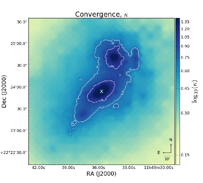
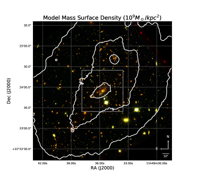
Figure 2.— Top: Convergence ($\kappa$) map for $z_{s}=9$ over the HST ACS field of view ($202\times 202\farcs$). The convergence reveals an elliptical total mass distribution with two major peaks, one occurring at the BCG and one occurring at a group of galaxies to the northwest of the BCG. The differences in effective resolution across regions are evident in this image — regions toward the outskirts of the modeling region are more pixellated than those near the BCG, as discussed in section 3.2. Note that this image employs a logarithmic stretch, and colorbar values show $\mathrm{log}_{10}(\kappa$). Contours shown correspond to $\kappa=5$ and $\kappa=10$. The cluster BCG is labelled with a white x. Bottom: Mass surface density contours for our mass model over the HST ACS field of view. Contours correspond to mass surface density values of 0.5, 1.0, and 2.0 $\times 10^{9}M_{\odot}/\textrm{kpc}^{2}$.

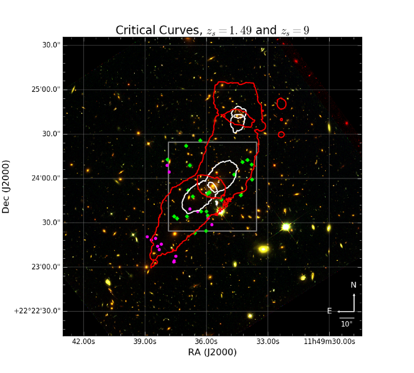
Figure 3.— Critical curves for redshifts $z_{s}=1.49$ (white), the redshift of SN Refsdal, and $z_{s}=9$ (red), over the HST ACS field of view ($202\times 202\farcs$). Multiple image locations are shown; green points are spectroscopically-confirmed images and magenta points correspond to images with photometric redshifts only. The multiple images are listed in Table 1. A zoomed-in image comparing this model’s critical curves at $z_{s}=1.49$ to other modelers’ critical curves is shown in Figure 4; its spatial extent is given by the gray box.

In our model, we use all gold images and most silver images, differing from those teams who created gold-only models (Grillo et al., 2016; Kawamata et al., 2016; Sharon & Johnson, 2015, Zitrin et al, in prep) or models that used all gold and silver images (Diego et al., 2016; Kawamata et al., 2016; Sharon & Johnson, 2015, note two teams created a model for each set of multiple images). We also reconstruct our mass model on an adaptive grid using weak lensing as input, which prominently differs from all modeling techniques discussed in Treu et al. (2016). Despite these distinctive inputs and modeling procedure, our model’s critical curves closely match those of the other groups in the Treu et al. (2016) collaboration (Figure 4, reflecting the strength of the constraints available to model this cluster.

We note that the constraints to the model in the central regions of the cluster are strong, but there are few constraints in the northwest region, the location of the object MACS1149-JD (Zheng et al., 2012). An analysis of this object, including our model’s estimates for its magnification, will be presented in a forthcoming paper (Hoag et al. 2017, in prep).

The overall root-mean-square (RMS) offset for the images, including both strongly-lensed background galaxy images and star-forming regions of the host galaxy for SN Refsdal, is $1^{\prime\prime}$, competitive with other models for the cluster (Treu et al., 2016). While it would be possible for our methodology to yield an RMS of $0^{\prime\prime}$, we tune the regularization parameter $\eta$ to prevent this outcome so as to avoid overfitting to noise.

At redshift $z_{s}=1.49$ (the redshift of SN Refsdal) we are able to closely reproduce the positions of the knots of the spiral host galaxy of SN Refsdal, although unlike parametric models, the effective resolution of our model ($0\farcs 3$/pixel) is too low to resolve the mass of the host galaxy in sufficient detail. Thus, we are unable to accurately determine the critical curves around the galaxy-scale lensing of SN Refsdal (images S1, S2, S3, and S4, see Table 2), or to make reliable predictions of the time delay between SN Refsdal images. Despite these limitations related to our effective resolution that prohibit us from making estimates based on fine-scale details of the cluster model, we have confidence in the large-scale shape of the model (Figure 4).

As a response to an STScI call to model the HFF clusters before and after the arrival of HFF data, this code was previously used to model MACS1149 using CLASH data. We compare our current (v3) model with the previous (v1) model using CLASH data. Note that some groups presented models in between the two official calls, which they denoted as v2; we did not create a v2 model. In the previous model, we used only 38 multiple images (14 systems), two of which (systems 8 and 12) have since been proven with spectroscopy to be spurious identifications. With updated imaging and spectroscopic data, the current version of the lensing model (v3) is substantially different from the previous model, much more similar to the other models (Figure 4) produced with the same post-HFF data. All maps of convergence, shear, and magnification, from this modeling team and other teams, are included in the Mikulski Archive for Space Telescopes (MAST, see footnote 7).

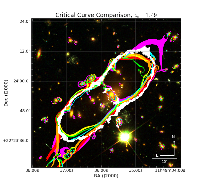
Figure 4.— A comparison of our critical curves at $z_{s}=1.49$ (white) with those of Diego et al. (2016, magenta), Grillo et al. (2016, red), Kawamata et al. (2016, orange, all images model), Jauzac et al. (2016, yellow), Sharon & Johnson (2015, cyan, gold-only model), and Zitrin et al. (in prep, green). The general shape of these modelers’ critical curves is in close agreement with those produced by our model. The critical curves shown are created by filling in regions of high magnification; the thickness of the curves depends on each model’s resolution. The field of view for this image is $60\farcs\times 60\farcs$, and is indicated by the gray square in Figure 3.

To determine the error in our model associated with photometric redshift uncertainty or incorrect system labels, we resample from the photometric redshift probability density functions $P_{i}(z_{\rm{Bayes}})$ produced by EAZY. We allow resampled photometric redshifts to have values $z_{\rm{phot}}<z_{\rm{cluster}}$, to account for the possibility of catastrophic errors. Although system redshift estimates may vary during this resampling, images belonging to a single system are always modeled as having a single redshift. After resampling the photometric systems, we run the modeling code again, and find that varying redshift estimates for photometric systems in the model produces errors within the range we have quoted.

We also determine the uncertainty associated with choice of weak lensing galaxies and SN Refsdal host galaxy star-forming regions using a bootstrap-resampling procedure that randomly weights the weak lensing and Refsdal system inputs. After this bootstrapping, we remodel the cluster with the bootstrapped values, and find that errors associated with our catalogs for weak lensing and SN Refsdal host galaxy star-forming regions are subdominant to the error associated with photometric redshifts. Nevertheless, we propagate all of these sources of error into the final errors for all lensed quantities. Additionally, we did vary the initial model, and found the results converge within error bars given by bootstrap estimates.

We assume any error in spectroscopic redshifts is small in comparison to modeling uncertainties, and we do not fully account for all possible sources of systematic error, such as choice of initial mass model, choice of refinement grid, spectroscopic redshift error, choice of regularization parameter, or spectroscopic image identification error.

4. Stellar Mass to Total Mass Ratio

4.1. Details of the Stellar Mass Density Map

We estimate the stellar mass density of MACS1149 with measurements of the approximate rest-frame K-band flux from the cluster members and a mass-to-light ratio, in the same manner as Hoag et al. (2016). We summarize this procedure in the following section.

We determine cluster membership using the catalog produced by Morishita et al. (2017a). We use 123 spectroscopic cluster members obtained from the public catalog of Ebeling et al. (2014), and 530 cluster members chosen using the photometric redshifts with informative prior presented by Morishita et al. (2017a), for a total of 591 cluster galaxies. Cluster member galaxies must obey the selection criterion $\delta z\equiv|z-z_{cls}|/(1+z_{cls})<\delta z_{cut}$, where $z_{cls}$ is the redshift of the cluster and $z$ is the redshift of each object. The cutoff redshift range $\delta z_{cut}=0.0084$ for those galaxies chosen from the Ebeling et al. (2014) spectroscopic catalog, and $\delta z_{cut}=0.0219$ for galaxies chosen by photometric redshift. (The average photo-z error is $\sigma_{z}=0.0073$, so this is a $3\sigma$ cutoff value.) Our catalog, which primarily consists of photometrically-determined cluster members, is much larger than the primarily spectroscopically-determined cluster catalog of Grillo et al. (2016), ensuring that we incorporate all cluster light into our estimates for stellar mass surface density, down to a completeness limit of $\textrm{log}M_{\star}/M_{\odot}=7.8$. An unsmoothed light map of the catalog is shown in Figure 5.

To measure the flux from the cluster members, a mask is created to eliminate all light in Spitzer/IRAC channel 1 that is not associated with a cluster member, and then we convolve with a one-pixel Gaussian kernel to smooth over the mask boundary. This rest-frame luminosity map is converted into a stellar mass surface density map using the mass-to-light ratio determined by Bell et al. (2003) using their ”diet-Salpeter” initial mass function (IMF). We use the mass-to-light ratio $M_{\star}/L=(0.83\pm 0.26)M_{\odot}/L_{\odot}$, which corresponds to the $10<$ log$(M_{\star}h^{2})<10.5$ stellar mass bin of the analysis by Bell et al. (2003). Note that given the substantial differences in $M_{\star}/L$ ratio between IMFs, our choosing an IMF introduces the largest source of systematic uncertainty, as large as $\delta f_{\star}=0.005$. While this uncertainty is large, we note that this approach to choosing the IMF is standard in SED fitting (Bell et al., 2003; Ilbert et al., 2010, 2013; Muzzin et al., 2013; Tomczak et al., 2014, 2017). It is also possible the IMF may differ across galaxies in the cluster. While we do not account for this source of error, we note that the massive, early-type galaxies in the cluster center are more likely to exhibit an IMF closer to Salpeter (Auger et al., 2010). As a result, we anticipate that the central peak in the stellar mass density map would be enhanced if we were to model dominant galaxies with a heavier IMF.

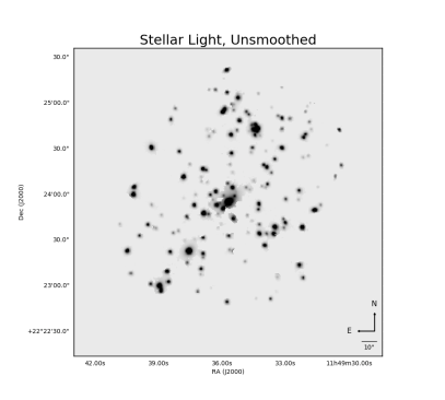
Figure 5.— Unsmoothed light map of the cluster members used in the creation of the $f_{\star}$ map. We use a cluster membership procedure based on astrometric matching and redshift cuts to create a cluster member catalog of 591 cluster galaxies. This light map is subsequently smoothed and compared to the mass model map to produce a map of the stellar to total mass ratio ($f_{\star}$, Figure 6)

Further, we adopt conservatively-large error bars on this mass-to-light ratio, using the spread of the $M_{\star}/L$ distribution as our statistical uncertainty on the $M_{\star}/L$ ratio rather than using the width of the most likely mean $M_{\star}/L$ bin (Bell et al., 2003). This choice accounts for possible correlation between the $M_{\star}/L$ ratios of galaxies in a single cluster, for a fixed IMF. Typically, when finding an average parameter value in a binned distribution of parameter means, it is appropriate to choose the width of the bin as the value for the statistical uncertainty. However, if the $M_{\star}/L$ ratios of galaxies in MACS1149 cluster were correlated, this approach would be insufficient to capture the uncertainty of the estimate, since galaxy $M_{\star}/L$ ratios could deviate from the mean in a related fashion. Thus, we must account for the spread of all possible $M_{\star}/L$ ratios to make a conservative estimate on the $M_{\star}/L$ ratios for these galaxies. In doing so, we incorporate a $\sim 30\%$ statistical uncertainty on our $M_{\star}/L$ ratio into our estimates, an uncertainty which dominates the statistical error in the stellar mass density model. This $\sim 30\%$ uncertainty accounts for possible variation of $M_{\star}/L$ of individual cluster members; this error is in addition to the systematic error associated with the choice of IMF.

To account for the additional stellar mass associated with the intracluster light (ICL), we increase the stellar mass surface densities across the map using the $8^{+12}_{-4}$% ICL mass estimate for MACS1149 by Morishita et al. (2017b). We propagate the errors in the ICL through to the final stellar mass surface density map. However, the effect of the ICL is still subdominant to both the statistical error on the $M_{\star}/L$ ratio and the systematic error associated with choosing an IMF in determining the uncertainty of the stellar mass surface density map. We do not account for possible radial gradients in the ICL. Morishita et al. (2017b) have noted that the ICL in MACS1149 is centrally concentrated with a shallow slope to $R<200$ kpc from the cluster center. Thus, we expect any radial gradients in the ICL to enhance the central peak in the stellar mass density map.

We also acknowledge that our procedure for choosing cluster members introduces the possibility of impurities in the catalog construction. However, we do not expect a spatial variation in these impurities, and thus anticipate that they would not effect our overall conclusions beyond a small bias factor in the stellar to total mass ratio.

To determine statistical errors in the maps, we resample from a Gaussian distribution for $M_{\star}/L$ with mean and standard deviation given by the distribution in Bell et al. (2003). We then use a resampling procedure to find the variation in the total mass surface density maps, and multiply the stellar mass surface density maps with an ICL resampled from the distribution from Morishita et al. (2017b) to yield a set of final error maps.

4.2. Details of the $f_{\star}$ Map

In our modeling approach, we do not directly assume that stellar light traces dark matter mass. The total mass distribution derived using our model is not strictly coupled to the stellar mass distribution. Therefore, it is informative to compare the spatial distribution of the ratio of stellar mass to total mass, $f_{\star}$. We further define the average ratio of the stellar mass to the total mass in an aperture as $\langle f_{\star}\rangle$.

To produce a projected $f_{\star}$ map, we match the mass resolution of the stellar mass density map with that of our model-constructed total mass density map, which has non-uniform mass resolution due to our method of refinement. To match the stellar mass density resolution to that of the total mass density map, we create five stellar mass surface density maps of different resolutions by convolving with five different Gaussian kernels of width corresponding to each of our five different levels of refinement. We use the best-fit kernel width of $0\farcm 74$ for the level of lowest refinement, as empirically determined by Hoag et al. (2016). The map corresponding to the second-lowest level of refinement is convolved with a Gaussian kernel with half the width of the kernel for the lowest level of refinement, and each subsequent level is convolved with a kernel smaller by a factor of two than the previous level of refinement. We then add the maps, weighting the pixels of each map by their locations on the refinement grid.

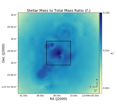
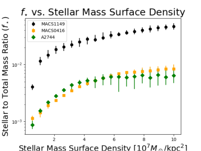
Figure 6.— Top: Spatial distribution of projected stellar mass to total mass ratio ($f_{\star}$). The center of the cluster has a value approaching $f_{\star}=5\%$, and the $f_{\star}$ value decreases with increasing distance from the mass concentrations in the cluster. Note that this image employs a logarithmic stretch, and colorbar values show $\mathrm{log}_{10}(f_{\star}$). The spatial extent of Figure 4 is given by the black box. Bottom: Stellar mass to total mass ratio within our field of view ($\langle f_{\star}\rangle$) vs. stellar mass surface density (in units of $10^{7}M_{\odot}/\rm{kpc}^{2}$), for the clusters MACS1149 (black circles), MACS0416 (orange squares, Hoag et al., 2016) and A2744 (green diamonds, Wang et al., 2015). Given the complexity of these clusters’ substructures and ambiguities in precisely defining the cluster center, this depiction of $\langle f_{\star}\rangle$ across varying physical scales is more reliable than a plot of $\langle f_{\star}\rangle$ vs. aperture size. Almost uniformly, in regions with higher stellar mass surface density there is a higher stellar mass fraction, particularly near the cluster core. MACS0416 and A2744 in general have much lower values of $\langle f_{\star}\rangle$ at these stellar mass surface densities. Note that these values are plotted logarithmically.

The final $f_{\star}$ map is created by taking the ratio of the resolution-corrected stellar mass surface density map to the total mass surface density map created by our model; this map is shown in Figure 6. To obtain the errors in $f_{\star}$, we resample the total mass surface density maps from our model, and create stellar mass surface density error maps by resampling from distributions of $M_{\star}/L$ ratios and ICL mass fractions. We use these to determine all errors in quantities derived from these maps.

We find $\langle f_{\star}\rangle=0.012^{+0.004}_{-0.003}$ when we average over a circular aperture, centered on the BCG, with a radius of 0.3 Mpc. If we use a Chabrier or Salpeter IMF, our $\langle f_{\star}\rangle$ values are $0.016^{+0.006}_{-0.005}$ (for a Salpeter IMF) or $0.010\pm 0.003$ (for a Chabrier IMF). We compare this value with other values for $\langle f_{\star}\rangle$ recently obtained in the literature. Using the same SWUnited modeling package to determine the total mass distribution, Hoag et al. (2016) produced maps for the cluster MACS 0416.1-2403 ($z=0.397$, MACS0416 hereafter); using these maps and our updated stellar mass map smoothing procedure, we find $\langle f_{\star}\rangle=0.005\pm 0.001$ in a circle of radius 0.3 Mpc. Similarly, using the SWUnited maps of Abell 2744 ($z=0.308$, A2744 hereafter) created by Wang et al. (2015), in a radius of 0.3 Mpc we find a value of $\langle f_{\star}\rangle=0.003\pm 0.001$. While these values are different than the original published values for $\langle f_{\star}\rangle$ due to our improved treatment of the stellar mass maps, they are still consistent with the original values within error bars. Notably, the model of MACS1149 predicts twice as much total mass as the models for MACS0416 or A2744, while all the clusters have comparable stellar mass estimates.

In another study of MACS0416, Jauzac et al. (2016) obtain a value of $\langle f_{\star}\rangle=0.0315\pm 0.0057$, using a smaller field of view and a Salpeter IMF rather than the diet-Salpeter IMF used in this work. If we re-calculate our value of $\langle f_{\star}\rangle$ for MACS1149 using a Salpeter IMF and the field of view used in Jauzac et al. (2016), we obtain an average stellar to total mass ratio of $0.044^{+0.015}_{-0.012}$, consistent with the value obtained by Jauzac et al. (2016) for a different, but similarly complex, cluster.

We also compare the distribution of stellar mass fraction across the cluster. We find that $f_{\star}$ peaks toward the center of the cluster. This suggests that the stellar mass surface density of MACS1149 peaks more sharply near the cluster center than the total surface mass density, i.e., that the stellar mass comprises a larger fraction of the total mass in the cluster center than on its outskirts. This effect would be enhanced with use of a heavier IMF, radial gradients in IMFs due to heavier masses in the central, dominant galaxies (Auger et al., 2010), and radial gradients in the ICL that concentrate in the center of the cluster (Morishita et al., 2017b). The value of $f_{\star}$ near the BCG is also very sensitive the procedure used for smoothing the stellar mass map (see Figure 9, Hoag et al., 2016). Outside the center of the cluster, we find the mass-rich northwest association of galaxies, which demonstrates a strong dark matter component in the convergence map (Figure 2), has a much lower $f_{\star}$ value than the other dark matter peaks, though the uncertainty of the total mass model in this region is much higher than in other regions due to relative lack of multiple images.

In addition to the inherent differences between clusters and possible projection effects, we have better model constraints near the cluster center for MACS1149 than were available for the analyses of A2744 and MACS0416 (Wang et al., 2015; Hoag et al., 2016). Hoag et al. (2016) demonstrated large systematic errors in $f_{\star}$ associated with smoothing. The original Wang et al. (2015) analysis did not undertake any smoothing of the stellar mass surface density map, and the Hoag et al. (2016) analysis had few multiple images near the cluster center, leading to large uncertainties in the smoothing in the center. In this work, because of the presence of SN Refsdal and its highly-resolved spiral host galaxy near the center of the cluster, we have a much higher resolution in this region. Thus, our analysis improves the smoothing methods developed by Hoag et al. (2016); Wang et al. (2015), and we consider our conclusions about $f_{\star}$ to be more robust, particularly in the center of the cluster.

In a study of baryon mass fractions in high-mass structures, Gonzalez et al. (2013) measured $f_{\star}$ for twelve dynamically relaxed galaxy clusters chosen from the X-ray sample of Gonzalez et al. (2007), with redshifts $z<0.3$. For clusters more massive than $2\times 10^{14}M_{\odot}$, within an aperture of $r_{500}$, they find a typical value of $\langle f_{\star}\rangle$ below 2%, consistent with our results.

Gonzalez et al. (2013) also discuss the stellar mass fraction relative to the cosmic baryon fraction value ($\frac{\Omega_{b}}{\Omega_{m}}$) and the ratio of stellar mass to gas mass ($\frac{f_{\star}}{f_{g}}$). Since most cluster baryon mass is comprised of intracluster gas, these values may be used to understand a cluster’s integrated star formation efficiency. Gonzalez et al. (2013) find that for clusters with total mass $\sim 10^{15}M_{\odot}$, the value of $\frac{f_{\star}}{f_{g}}\approx 0.1$ out to a radius of $r_{500}$. Using the value of $r_{500}$ and gas mass estimate of MACS1149 found by Mantz et al. (2010) and the mass-to-light ratio assumed in Gonzalez et al. (2013), we model the stellar mass out to $r_{500}$ ($1.53\pm 0.08\rm{Mpc}$, $4.00\pm 0.21\farcm$) by assuming a Gaussian distribution of stellar mass surface density over large scales, centered on the peak stellar mass surface density. We find a stellar mass fraction of $\sim 2\%$, and a value of $\frac{f_{\star}}{f_{g}}\approx 0.16$. These values are broadly consistent with the results of Gonzalez et al. (2013). We also calculate a cluster baryon fraction value of $\frac{\Omega_{b}}{\Omega_{m}}\approx 13\%$, and compare to the Planck value of $\frac{\Omega_{b}}{\Omega_{m}}=15.6\pm 3.6\%$. (Planck Collaboration, 2016)

Our results are also consistent with those of Ascaso et al. (2014), who used a method that does not rely on lensing and a Chabrier IMF to establish $f_{\star}=0.00426$ at $z=0.1$ and $f_{\star}=0.00398$ at $z=1$, for $R<R_{\rm{vir}}$. This suggests that the integrated star formation efficiency for MACS1149 is within the typical range for massive clusters, and within the uncertainties is consistent with a relaxed cluster with a typical star formation history integrated from $z_{\rm{formation}}$.

5. Conclusions

The galaxy cluster MACS1149 is a complex merging cluster with a multiply lensed spiral galaxy hosting a supernova. We use 38 independent multiple images of background galaxies corresponding to 13 total systems, and an additional 100 images corresponding to 31 star-forming regions in the SN Refsdal host galaxy. Using these constraints and an adaptive grid reconstruction method that combines strong and weak lensing, we produce a mass model of this cluster, which yields critical curves with a general shape that closely agrees with those of other current cluster lens models of MACS1149.

We present a stellar mass surface density map using Spitzer/IRAC data, and compare this map to the total mass density obtained from our lens model to obtain a map of the projected stellar mass to total mass ratio, $f_{\star}$. We find that for MACS1149, stellar mass tends to be more concentrated toward the cluster BCG, compared to the distribution of total mass (stellar + gas + dark matter). We obtain a mean stellar mass fraction $\langle f_{\star}\rangle=0.012^{+0.004}_{-0.003}$ within 0.3 Mpc of the BCG, which is somewhat higher than the average stellar mass fraction of two other HFF clusters studied (MACS0416 and A2744), but broadly consistent with other estimates of this ratio. Discrepancies between the values of $f_{\star}$ between clusters can be explained by differences in smoothing techniques used, as well as by the natural variation between clusters. Moreover, this stellar mass fraction is consistent with the range of integrated star formation efficiency values for massive clusters of $z<1$.

Additionally, both the mass model and the $f_{\star}$ map provide valuable clues for the ongoing discussions of how stellar light traces mass. We find that, in general, the stellar light in MACS1149 traces its mass, with a substantial dark matter peak near the cluster BCG. While a single cluster cannot on its own speak to these larger theoretical questions, the results observed for MACS1149 can be combined with those of other clusters to yield insight into the LTM assumption, and the various theories that rest upon it.

References

- Ascaso et al. (2014) Ascaso, B., Lemaux, B. C., Lubin, L. M., et al. 2014, MNRAS, 442, 589
- Atek et al. (2014) Atek, H., Richard, J., Kneib, J.-P., et al. 2014, ApJ, 786, 60
- Atek et al. (2015) Atek, H., Richard, J., Kneib, J.-P., et al. 2015, ApJ, 800, 18
- Auger et al. (2010) Auger, M. W., Treu, T., Gavazzi, R., et al. 2018, ArXiv e-prints, 1007.2409
- Bacon et al. (2010) Bacon, R., Accardo, M., Adjali, L., et al. 2010, The MUSE Second-Generation VLT Instrument, Proc. SPIE, 7735, 773508
- Bahcall et al. (1995) Bahcall, N. A., Lubin, L. M., & Dorman, V., 1995, ApJ, 447, L81
- Bahcall & Kulier (2014) Bahcall, N. A. & Kulier, A., 2014, MNRAS, 439, 2505
- Behroozi et al. (2013) Behroozi, P. S., Wechsler, R. H., & Conroy, C., 2013, ApJ, 770, 57
- Bell et al. (2003) Bell, E. F., McIntosh, D. H., Katz, N., et al. 2003, ApJS, 149, 289
- Bertin & Arnouts (1996) Bertin, E. & Arnouts, S., 1996, A&AS, 117, 393
- Bouwens et al. (2014) Bouwens, R. J., Bradley, L., Zitrin, A., et al. 2014, ApJ, 795, 126
- Bouwens et al. (2016) Bouwens, R. J., Oesch, P. A., Illingworth, G. D., et al. 2016, ApJ, 843, 129
- Bradač et al. (2005) Bradač, M., Schneider, P., Lombardi, M., Erben, T. 2005, A&A, 437, 39
- Bradač et al. (2009) Bradač, M., Treu, T., Applegate, D., et al. 2009, ApJ, 706, 1201
- Bradač et al. (2014) Bradač, M., Ryan, R., Casertano, S., et al. 2014, ApJ, 785, 108
- Bradley et al. (2014) Bradley, L. D., Zitrin, A., Coe, D., et al. 2014, ApJ, 792, 76
- Brammer et al. (2008) Brammer, G. B., van Dokkum, P. G., & Coppi, P. 2008, ApJ, 686, 1503
- Kelly et al. (2016) Kelly, P. L., Brammer, G., Selsing, J., et al. 2016, ApJ, 831, 205
- Budzynski et al. (2014) Budzynski, J. M., Koposov, S. E., McCarthy, I. G., et al. 2014, MNRAS, 437, 1362
- Chabrier (2003) Chabrier, G., 2003, PASP, 115, 763
- Christensen et al. (2012) Christensen, L., Laursen, P., Richard, J., et al. 2012, MNRAS, 427, 1973
- Clowe et al. (2006) Clowe, D. Bradač, M., Gonzalez, A. H., et al. 2006, ApJ, 648, L109
- Coe et al. (2013) Coe, D., Zitrin, A., Carrasco, M., et al. 2013, ApJ, 762, 32
- Coe et al. (2015) Coe, D., Bradley, L., & Zitrin, A., 2015, ApJ, 800, 84
- Dahlen et al. (2013) Dahlen, T., Mobasher, B., Faber, S. M., et al. 2013, ApJ, 775, 93
- De Lucia et al. (2004) De Lucia, G., Kauffmann, G., & White, S. D. M., 2004, MNRAS, 349, 1101
- Diego et al. (2016) Diego, J. M., Broadhurst, T., Chen, C., et al. 2016, MNRAS, 456, 356
- Dolag et al. (2009) Dolag, K., Borgani, S., Murante, G., et al. 2009, MNRAS, 399, 497
- Dubois et al. (2013) Dubois, Y., Pichon, C., Devriendt, J., et al. 2013, MNRAS, 428, 2885
- Ebeling et al. (2001) Ebeling, H., Edge, A. C., & Henry, J. P., 2001, ApJ, 553, 668
- Ebeling et al. (2014) Ebeling, H., Ma, C. J., & Barrett, E., 2014, ApJS, 211, 21
- Erben et al. (2001) Erben, T., Van Waerbeke, L., Bertin, E., et al. 2001, A&A, 366, 717
- Ettori et al. (2006) Ettori, S., Dolag, K., Borgani, S., et al. 2006, MNRAS, 365, 102
- Gonzalez et al. (2007) Gonzalez, A. H., Zaritsky, D., & Zabludoff, A. I., 2007, ApJ, 666, 147
- Gonzalez et al. (2013) Gonzalez, A. H., Sivanandam, S., Zabludoff, A. I., et al. 2013, ApJ, 778, 14
- Grillo et al. (2016) Grillo, C., Karman, W., Suyu, S. H., et al. 2016, ApJ, 822, 78
- Guo et al. (2013) Guo, Y., Ferguson, H. C., Giavalisco, M., et al. 2013, ApJS, 207, 24
- Hoag et al. (2016) Hoag, A., Huang, K., Treu, T., et al. 2016, ApJ, 831, 182
- Hoekstra et al. (1998) Hoekstra, H., Franx, M., Kuijken, K., et al. 1998, ApJ, 504, 636
- Huang et al. (2016) Huang, K.-H., Bradač, M., Lemaux, B. C., et al. 2016b, ApJ, 817, 11
- Ilbert et al. (2010) Ilbert, O., Salvato, M., Le Floc’h, E., et al. 2010, ApJ, 709, 644
- Ilbert et al. (2013) Ilbert, O., McCracken, H. J., Le Fevre, O., et al. 2013, A&A, 556, A55
- Ishigaki et al. (2017) Ishigaki, M., Kawamata, R., Ouchi, M., et al. 2017, ArXiv e-prints, 1702.04867
- Jauzac et al. (2012) Jauzac, M., Jullo, E., Kneib, J. P., et al. 2012, MNRAS, 426, 3369
- Jauzac et al. (2016) Jauzac, M., Richard, J., Limousin, M., et al. 2016, MNRAS, 457, 2029
- Johnson et al. (2014) Johnson, T. L., Sharon, K., Bayliss, M. B., et al 2014, ApJ, 797, 48J
- Johnson & Sharon (2016) Johnson, T. L. & Sharon, K. 2016, ArXiv e-prints, 1608.08713
- Jones et al. (2010) Jones, T. A., Swinbank, A. M., Ellis, R. S., et al. 2010, MNRAS, 404, 1247
- Jones et al. (2015) Jones, T. A., Wang, X., Schmidt, K. B., et al. 2015, AJ, 149, 3
- Kaiser et al. (1995b) Kaiser, N., Squires, G., & Broadhurst, T., 1995, ApJ, 449, 460
- Karman et al. (2016) Karman, W., Grillo, C., Balestra, I., et al. 2016, A&A, 585, A27
- Kawamata et al. (2016) Kawamata, R., Oguri, M., Ishigaki, M., et al. 2016, ApJ, 819, 114
- Kelly et al. (2015) Kelly, P. L., Rodney, S. A., Treu, T., et al. 2015, Science, 347, 6226, 1123
- Kelly et al. (2016) Kelly, P. L., Rodney, S. A., Treu, T., et al. 2016, ApJ, 819, L8
- Koester et al. (2007a) Koester, B. P., McKay, T. A., Annis, J., et al. 2007, ApJ, 660, 221
- Koester et al. (2007b) Koester, B. P., McKay, T. A., Annis, J., et al. 2007, ApJ, 660, 239
- Kravtsov et al. (2005) Kravtsov, A., Nagai, D., & Vikhlinin, A. A., 2005, ApJ, 625, 588
- Kravtsov et al. (2014) Kravtsov, A., Vikhlinin, A., & Meshscheryakov, A., 2014, ArXiv e-prints, 1401.7329
- Kron (1980) Kron, R. G., 1980, ApJS, 43, 305
- Laporte & White (2015) Laporte, C. F. P. & White, S. D. M. 2015, MNRAS, 451, 1177
- Leethochawalit et al. (2016) Leethochawalit, N., Jones, T. A., Ellis, R. S., et al. 2016, ApJ, 820, 84
- Lemaux et al. (2012) Lemaux, B. C., Gal, R. R., Lubin, L. M., et al. 2012, ApJ, 745, 106
- Lin et al. (2003) Lin, Y. T., Mohr, J. J., & Stanford, S. A., 2003, ApJ, 591, 749
- Livermore et al. (2017) Livermore, R. C., Finkelstein, S. L., & Lotz, J. M., 2017, ApJ, 835, 113
- Lotz et al. (2016) Lotz, J. M., Koekemoer, A., Coe, D., et al. 2016, ArXiv e-prints, 1605.06567
- Luppino & Kaiser (1997) Luppino, G. A. & Kaiser, N., 1997, ApJ, 475, 20
- Mantz et al. (2010) Mantz, A., Allen, S. W., Ebeling, H., et al. 2010, MNRAS, 406, 1773
- Markevitch et al. (2004) Markevitch, M., Gonzalez, A. H., Clowe, D., et al. 2004, ApJ, 606, 819
- Martizzi et al. (2014) Martizzi, D., Jimmy, Teyssier, R., et al. 2014, MNRAS, 443, 1500
- Mason et al. (2016) Mason, C. A., Treu, T., Fontana, A., et al. 2016, ArXiv e-prints, 1610.03075
- Massey et al. (2014) Massey, R., Schrabback, T., Cordes, O., et al. 2014, MNRAS, 439, 887
- Merlin et al. (2015) Merlin, E., Fontana, A., Ferguson, H. C., et al. 2015, A&A, 582, A15
- Mohammed et al. (2016) Mohammed, I., Saha, P., Williams, L. L. R., et al. 2016, MNRAS, 459, 1698
- Morishita et al. (2017a) Morishita, T., Abramson, L. E., Treu, T., et al. 2017, ApJ, 835, 254
- Morishita et al. (2017b) Morishita, T., Abramson, L. E., Treu, T., et al. 2017, ApJ, 846, 139
- Muzzin et al. (2013) Muzzin, A., Marchesini, D., Stefanon, M., et al. 2013, ApJ, 777, 18
- Nagai et al. (2007) Nagai, D., Vikhlinin, A., & Kravtsov, A. V., ApJ, 655, 98
- Natarajan et al. (2017) Natarajan, P., Chadayammuri, U., Jauzac, M., et al. 2017, ArXiv e-prints, 1702.04348
- Oguri (2015) Oguri, M., 2015, MNRAS, 449, L86
- Oke (1974) Oke, J. B. 1974, ApJS, 27, 21
- Planck Collaboration (2016) Planck Collaboration, Ade, P. A. R., Aghanim, N., et al. 2016, A&A, 594, A13
- Postman et al. (2012) Postman, M., Coe, D., Benítez, N., et al. 2012, ApJS, 199, 25
- Press (1997) Press, W. H., 1997, Unsolved Problems in Astrophysics, ed. J N. Bahcall & J. P. Ostriker, 49-60
- Priewe et al. (2017) Priewe, J., Williams, L. L. R., Liesenborgs, J., et al. 2017, MNRAS, 465, 1030
- Rau et al. (2014) Rau, S., Vegetti, S., & White, S. D. M., 2014, MNRAS, 443, 957
- Refsdal (1964) Refsdal, S., 1964, MNRAS, 128, 307
- Richard et al. (2011) Richard, J., Jones, T., Ellis, R., et al. 2011, MNRAS, 413, 643
- Richard et al. (2014) Richard, J., Jauzac, M., Limousin, M., et al. 2014, MNRAS, 444, 268
- Robertson et al. (2013) Robertson, B. E., Furlanetto, S. R., Schneider, E., et al. 2013, ApJ, 768, 71
- Robertson et al. (2015) Robertson, B. E., Ellis, R. S., Furlanetto, S. R., et al. 2015, ApJ, 802, L19
- Rodney et al. (2015a) Rodney, S. A., Patel, B., Scolnic, D., et al. 2015, ApJ, 811, 70
- Rodney et al. (2015b) Rodney, S. A., Strolger, L.-G., Kelly, P. L., et al. 2015, ApJ, 820, 50
- Ryan et al. (2014) Ryan, R. E. Jr., Gonzalez, A. H., Lemaux, B. C., et al. 2014, ApJ, 786, L4
- Salpeter (1955) Salpeter, E. E., 1955, ApJ, 121, 161
- Schmidt (2014) Schmidt, K. B., Treu, T., Brammer, G. B., et al. 2014, ApJ, 782, L36
- Schrabback et al. (2007) Schrabback, T., Erben, T., Simon, P., et al. 2007, A&A, 468, 823
- Schrabback et al. (2010) Schrabback, T., Hartlap, J., Joachimi, B., et al. 2010, A&A, 516, A63
- Schrabback et al. (2018a) Schrabback, T., Applegate, D., Dietrich, J. P., et al. 2018, MNRAS, 474, 2635
- Schrabback et al. (2018b) Schrabback, T., Schirmer, M., van der Burg, R. F. J., et al. 2018, ArXiv e-prints, 1711.00475
- Simionescu et al. (2011) Simionescu, A., Allen, S. W., Mantz, A., et al. 2011, Science, 331, 1576
- Sharon & Johnson (2015) Sharon, K. & Johnson, T. L., 2015, ApJ, 800, L26
- Smith et al. (2009) Smith, G. P., Ebeling, H., Limousin, M., et al. 2009, ApJ, 707, L163
- Stark et al. (2008) Stark, D. P., Swinbank, A. M., Ellis, R. S., et al. 2008, Nature, 455, 775
- Tomczak et al. (2014) Tomczak, A. R., Quadri, R. F., Tran, K.-V. H., et al. 2014, ApJ, 783, 85
- Tomczak et al. (2017) Tomczak, A. R., Lemaux, B. C., Lubin, L. M., et al. 2017, MNRAS, 472, 3512
- Treu et al. (2015) Treu, T., Schmidt, K. B., Brammer, G. B., et al. 2015, ApJ, 812, 114
- Treu et al. (2016) Treu, T., Brammer, G., Diego, J.M., et al. 2016, ApJ, 817, 60
- Valdarnini (2003) Valdarnini, R., 2003, MNRAS, 339, 1117
- Vulcani et al. (2016) Vulcani, B., Treu, T., Schmidt, K. B., et al. 2016, ApJ, 833, 178
- Wang et al. (2015) Wang, X., Hoag, A., Huang, K.-H., et al. 2015, ApJ, 811, 29
- Zheng et al. (2012) Zheng, W., Postman, M., Zitrin, A., et al. 2012, Nature, 489, 406
- Zitrin & Broadhurst (2009) Zitrin, A. & Broadhurst, T., 2009, ApJ, 703, L132
- Zitrin et al. (2011) Zitrin, A., Broadhurst, T., Barkana, R., et al. 2011, MNRAS, 410, 1939