Excessive Backlog Probabilities of Two Parallel Queues

Abstract

Let $X$ be the constrained random walk on ${\mathbb{Z}}_{+}^{2}$ with increments $(1,0)$, $(-1,0)$, $(0,1)$ and $(0,-1)$; $X$ represents, at arrivals and service completions, the lengths of two queues (or two stacks in computer science applications) working in parallel whose service and interarrival times are exponentially distributed with arrival rates $\lambda_{i}$ and service rates $\mu_{i}$, $i=1,2$; we assume $\lambda_{i}<\mu_{i}$, $i=1,2$, i.e., $X$ is assumed stable. Without loss of generality we assume $\rho_{1}=\lambda_{1}/\mu_{1}\geq\rho_{2}=\lambda_{2}/\mu_{2}$. Let $\tau_{n}$ be the first time $X$ hits the line $\partial A_{n}=\{x\in{\mathbb{Z}}^{2}:x(1)+x(2)=n\}$, i.e., when the sum of the components of $X$ equals $n$ for the first time. Let $Y$ be the same random walk as $X$ but only constrained on $\{y\in{\mathbb{Z}}^{2}:y(2)=0\}$ and its jump probabilities for the first component reversed. Let $\partial B=\{y\in{\mathbb{Z}}^{2}:y(1)=y(2)\}$ and let $\tau$ be the first time $Y$ hits $\partial B$. The probability $p_{n}=P_{x}(\tau_{n}<\tau_{0})$ is a key performance measure of the queueing system (or the two stacks) represented by $X$ (if the queues/stacks share a common buffer, then $p_{n}$ is the probability that this buffer overflows during the system’s first busy cycle). Stability of the process implies that $p_{n}$ decays exponentially in $n$ when the process starts off the exit boundary $\partial A_{n}.$ We show that, for $x_{n}=\lfloor nx\rfloor$, $x\in{\mathbb{R}}_{+}^{2}$, $x(1)+x(2)\leq 1$, $x(1)>0$, $P_{(n-x_{n}(1),x_{n}(2))}(\tau<\infty)$ approximates $P_{x_{n}}(\tau_{n}<\tau_{0})$ with exponentially vanishing relative error. Let $r=(\lambda_{1}+\lambda_{2})/(\mu_{1}+\mu_{2})$; for $r^{2}<\rho_{2}$ and $\rho_{1}\neq\rho_{2}$, we construct a class of harmonic functions from single and conjugate points on a related characteristic surface for $Y$ with which the probability $P_{y}(\tau<\infty)$ can be approximated with bounded relative error. For $r^{2}=\rho_{1}\rho_{2}$, we obtain the exact formula $P_{y}(\tau<\infty)=r^{y(1)-y(2)}+\frac{r(1-r)}{r-\rho_{2}}\left(\rho_{1}^{y(1)}-r^{y(1)-y(2)}\rho_{1}^{y(2)}\right).$

Keywords: approximation of probabilities of rare events, exit probabilities, constrained random walks, queueing systems, large deviations

1 Introduction

This work concerns the random walk $X$ with independent and identically distributed increments $\{I_{1},I_{2},I_{3},...\}$, constrained to remain in ${\mathbb{Z}}_{+}^{2}$:

$$X_{0} =x\in{\mathbb{Z}}_{+}^{2},~{}~{}~{}X_{k+1}\doteq X_{k}+\pi(X_{k},I_{k}),k=1,2,3,...$$

$$\pi(x,v) \doteq\begin{cases}v,&\text{ if }x+v\in{\mathbb{Z}}^{2}_{+},\\ 0,&\text{otherwise,}\end{cases}$$

$$I_{k}\in\{(1,0),(-1,0),(0,1),(0,-1)\},P(I_{k}=(1,0))=\lambda_{1},$$

$$P(I_{k}=(0,1))=\lambda_{2},P(I_{k}=(-1,0))=\mu_{1},P(I_{k}=(0,-1))=\mu_{2}.$$

The dynamics of $X$ are depicted in Figure 1.

Figure 1:    Dynamics of $X$

We denote the constraining boundaries by $\partial_{i}\doteq\{x\in{\mathbb{Z}}^{2}:x(i)=0\}$, $i=1,2$. A well known interpretation for $X$ is as the embedded random walk of two parallel queues with Poisson arrivals and independent and exponentially distributed service times. This random walk appears in computer science as a model of two stacks running together [42, 68, 32, 48]. Define the region

$$A_{n}=\left\{x\in{\mathbb{Z}}_{+}^{2}:x(1)+x(2)\leq n\right\}$$ (1)

and its boundary

$$\partial A_{n}=\left\{x\in{\mathbb{Z}}_{+}^{2}:x(1)+x(2)=n\right\}.$$ (2)

Let $\tau_{n}$ be the first time $X$ hits $\partial A_{n}$:

$$\tau_{n}\doteq\inf\{k:X_{k}\in\partial A_{n}\}.$$ (3)

When $X$ is stable, i.e., when $\lambda_{i}<\mu_{i}$, a well known performance measure associated with $X$ is the probability $p_{n}\doteq P_{x}(\tau_{n}<\tau_{0})$; if the queues share a common buffer, then $p_{n}$ is the probability that this buffer overflows during the system’s first busy cycle. The stability assumption implies that $p_{n}$ decays exponentially in $n$, when the walk starts away from the exit boundary $\partial A_{n}$. Hence $\{\tau_{n}<\tau_{0}\}$ is a rare event for $n$ large. There is no closed form formula for $p_{n}$ in terms of the parameters of the problem; the approximation of probabilities of the type $p_{n}$ and of related probabilities and expectations for constrained processes has been a challenge for many years and there is a wide literature on this subject using techniques including large deviations analysis and rare event simulation, see, [1, 2, 3, 5, 4, 6, 7, 8, 10, 9, 12, 13, 15, 16, 17, 18, 20, 21, 22, 23, 29, 25, 32, 34, 33, 35, 36, 19, 38, 37, 39, 41, 40, 58, 27, 43, 44, 45, 46, 47, 48, 49, 50, 51, 52, 53, 54, 26, 67, 14, 55, 56, 57, 59, 11, 60, 63, 64, 68, 30].

The goal of the present work is to prove, for the constrained random walk $X$ defined above, that the approximation approach used in [65, 66] gives approximations of $p_{n}$ with exponentially decaying relative error when the initial position $x$ of the random walk is off the boundary $\partial_{1}.$ The work [66, Section 6] reviews many of the works cited above and points out the relations between the approach of the current paper and [65, 66] and the range of methods and approaches used in these works.

The approximation technique and the proof method are reviewed below (see subsection 1.1). Although the main approach of the present work is parallel to that of [65, 66], new challenges and ideas appear in the treatment of the present case; there are also differences in the assumptions made and the results obtained. These are reviewed in Section 8.

First, several definitions; the utilization rates of the nodes are:

$$\rho_{i}=\frac{\lambda_{i}}{\mu_{i}},i=1,2.$$

We assume that $X$ is stable, i.e.,

$$\rho_{1},\rho_{2}<1.$$

The following quantity plays a central role in our analysis:

$$r=\frac{\lambda_{1}+\lambda_{2}}{\mu_{1}+\mu_{2}}.$$

Without loss of generality we can assume

$$\rho_{2}\leq r\leq\rho_{1}$$ (4)

(if this doesn’t hold, rename the nodes). We will make two further technical assumptions:

$$\rho_{1}\neq\rho_{2},\frac{r^{2}}{\rho_{2}}<1.$$ (5)

The first of these is needed in the construction of the $Y$-harmonic functions in Section 2, see (15). The second is useful both in the computation of $P_{y}(\tau<\infty)$ (see the proof of Proposition 7.2) and in the limit analysis (see the proof of Proposition 3.3). We further comment on these assumptions in the Conclusion (Section 9).

Define the linear transformation

$${\mathcal{I}}\doteq\left(\begin{matrix}-1&0\\ 0&1\end{matrix}\right)$$

and the affine transformation

$$T_{n}=ne_{1}+{\mathcal{I}}$$

where $(e_{1},e_{2})$ is the standard basis for ${\mathbb{R}}^{2}.$ Furthermore, define the constraining map

$$\pi_{1}(x,y)=\begin{cases}y,&\text{ if }x+y\in{\mathbb{Z}}\times{\mathbb{Z}}_{+},\\ 0,&\text{otherwise.}\end{cases}$$

Define $Y$ to be a constrained random walk on ${\mathbb{Z}}\times{\mathbb{Z}}_{+}$ with increments

$$J_{k}\doteq{\mathcal{I}}I_{k}:$$ (6)

$$Y_{k+1}=Y_{k}+\pi_{1}(Y_{k},J_{k}).$$

$Y$ has the same increments as $X$, but the probabilities of the increments $e_{1}$ and $-e_{1}$ are reversed. Define

$$\partial B\subset{\mathbb{Z}}\times{\mathbb{Z}}_{+},\partial B\doteq\left\{y:y(1)=y(2)\right\},$$

and the hitting time $\tau\doteq\inf\left\{k:Y_{k}\in\partial B\right\}.$

1.1 Summary of our analysis

[65, Proposition 3.1] asserts, in a more general framework than the model given above, that for any $y\in{\mathbb{Z}}_{+}^{2}$, $y(1)>y(2)$, $P_{T_{n}(y)}(\tau_{n}<\tau_{0})\rightarrow P_{y}(\tau<\infty)$. The approximation idea connecting these two probabilities is shown in Figure 2: by applying $T_{n}$, we move the origin of the coordinate system to $(n,0)$ and take limits, which leads to the limit problem of computing $P_{y}(\tau<\infty)$ where the limit $Y$ process is the same process as $X$ (observed from the point $(n,0)$) but not constrained on $\partial_{1}.$

Figure 2:    Transformations and the limit problem

A more interesting convergence analysis is when the initial point is given in $x$ coordinates. A convergence analysis from this point of view has only been performed so far for the constrained random walk with increments $(1,0)$, $(-1,1)$ and $(0,-1)$ (representing two tandem queues) in [65, 66]. The goal of the present work is to extend this analysis to the simple random walk $X$. Our main result is the following theorem:

Theorem (Theorem 6.1).

For any $x\in{\mathbb{R}}_{+}^{2}$, $x(1)+x(2)<1$, $x(1)>0$, there exists $C_{7}>0$ and $N>0$ such that

$$\frac{|P_{x_{n}}(\tau_{n}<\tau_{0})-P_{T_{n}(x_{n})}(\tau<\infty)|}{P_{x_{n}}(\tau_{n}<\tau_{0})}<e^{-C_{7}n}$$

for $n>N$, where $x_{n}=\lfloor xn\rfloor$.

Thus, as $n$ increases $P_{T_{n}(x_{n})}(\tau<\infty)$ approximates $P_{x_{n}}(\tau_{n}<\tau_{0})$ very well (with exponentially decaying relative error in $n$) if $x(1)>0.$ In the tandem case there is a simple explicit formula for $P_{y}(\tau<\infty)$. In the parallel walk case a simple explicit formula exists under the additional condition

$$\rho_{1}\rho_{2}=r^{2}.$$ (7)

The formula for $P_{y}(\tau<\infty)$ under this condition is

$$P_{y}(\tau<\infty)=r^{y(1)-y(2)}+\frac{(1-r)r}{r-\rho_{2}}\left(\rho_{1}^{y(1)}-r^{y(1)-y(2)}\rho_{1}^{y(2)}\right).$$ (8)

This is derived in Proposition 7.2 and is based on the class of $Y$-harmonic functions constructed in Section 2 from single and conjugate points on a characteristic surface associated with $Y$. A generalization of (58) can be used to find upper and lower bounds for $P_{y}(\tau<\infty)$ when (7) doesn’t hold, see Propositions 7.3 and 7.6. Subsection 7.1 illustrates how one can use these results to construct finer approximations of $P_{y}(\tau<\infty)$ with diminishing relative error using superposition of $Y$-harmonic functions defined by single and conjugate points on the characteristic surface.

Define the stopping times

$$\sigma_{1}=\inf\{k:X_{k}\in\partial_{1}\},~{}~{}~{}\bar{\sigma}_{1}=\inf\{k:T_{n}(Y_{k})\in\partial_{1}\}.$$ (9)

If we set the initial position of $Y$ to $Y_{0}=T_{n}(X_{0})$, we have

$$\{\tau_{n}<\tau_{0}\}\cap\{\tau_{n}<\sigma_{1}\wedge\tau_{0}\}=\{\tau<\infty\}\cap\{\tau<\bar{\sigma}_{1}<\infty\}.$$

The main argument in the proof of Theorem 6.1 is this: most of the probability of the events $\{\tau_{n}<\tau_{0}\}$ and $\{\tau<\infty\}$ come from the events $\{\tau_{n}<\sigma_{1}\wedge\tau_{0}\}$ and $\{\tau<\bar{\sigma}_{1}<\infty\}$ respectively, if the initial position $X_{0}$ of $X$ is away from $\partial_{1}.$ The full implementation of this argument will require the following steps:

1. Construction of $Y$-harmonic functions, $Y-z$ harmonic functions and bounds on ${\mathbb{E}}_{y}[z^{\tau}1_{\{\tau<\infty\}}]$ for $z>1$ (Sections 2 and 3),

2. Large deviations (LD) analysis of $P_{x_{n}}(\tau_{n}<\tau_{0})$ (Section 4),

3. LD analysis of $P_{x_{n}}(\sigma_{1}<\tau_{n}<\tau_{0})$ (Section 5),

4. LD analysis of $P_{x_{n}}(\bar{\sigma}_{1}<\tau<\infty)$ (Subsection 5.1).

These steps are put together in Section 6. Section 7 treats the problem of computing $P_{y}(\tau<\infty)$ from the $Y$-harmonic functions of Section 2. Section 8 points out the parallels and differences between the analysis of the constrained walk $X$ treated in the present work and the tandem walk treated in [65, 66]. We comment on future work in the conclusion (Section 9).

2 Harmonic functions of $Y$

A function $h$ on ${\mathbb{Z}}\times{\mathbb{Z}}_{+}$ is said to be $Y$-harmonic if

$${\mathbb{E}}_{y}[h(Y_{1})]=h(y),y\in{\mathbb{Z}}\times{\mathbb{Z}}_{+}.$$

Following [65], introduce the the interior characteristic polynomial of $Y$:

$${\bm{p}}(\beta,\alpha)\doteq\lambda_{1}\frac{1}{\beta}+\mu_{1}\beta+\lambda_{2}\frac{\alpha}{\beta}+\mu_{2}\frac{\beta}{\alpha}.$$

and characteristic polynomial of $Y$ on $\partial_{1}$:

$${\bm{p}}_{1}(\beta,\alpha)\doteq\lambda_{1}\frac{1}{\beta}+\mu_{1}\beta+\lambda_{2}\frac{\alpha}{\beta}+\mu_{2}$$

As in [65], we will construct $Y$-harmonic functions from solutions of ${\bm{p}}=1$; the set of all solutions of this equation defines the characteristic surface

$${\mathcal{H}}\doteq\{(\beta,\alpha)\in{\mathbb{C}}^{2}:{\bm{p}}(\beta,\alpha)=1\},$$

define, similarly, the characteristic surface for $\partial_{1}$:

$${\mathcal{H}}_{1}\doteq\{(\beta,\alpha)\in{\mathbb{C}}^{2}:{\bm{p}}_{1}(\beta,\alpha)=1\},$$

Multiplying both sides of ${\bm{p}}=1$ by $\alpha$ transforms it to the quadratic equation

$$\alpha\left(\lambda_{1}\frac{1}{\beta}+\mu_{1}\beta-1\right)+\lambda_{2}\frac{\alpha^{2}}{\beta}+\mu_{2}\beta=0,$$ (10)

Define

$$\boldsymbol{\alpha}(\beta,\alpha)\doteq\frac{1}{\alpha}\frac{\beta^{2}}{\rho_{2}};$$ (11)

if for a fixed $\beta$, $\alpha_{1}$ and $\alpha_{2}$ are distinct roots of (10), they will satisfy

$$\alpha_{2}=\boldsymbol{\alpha}(\beta,\alpha_{1})$$

by simple algebra; we will call the points $(\beta,\alpha_{1})\in{\mathcal{H}}$ and $(\beta,\alpha_{2})\in{\mathcal{H}}$ arising from such roots conjugate. Following [65] we refer to the function $\boldsymbol{\alpha}$ as the conjugator. An example of two conjugate points are shown in Figure 3.

Figure 3: The real section of the characteristic surface ${\mathcal{H}}$ for $\lambda_{1}=0.15$, $\lambda_{2}=0.2$, $\mu_{1}=0.25$, $\mu_{2}=0.4$; the end points of the dashed line are an example of a pair of conjugate points $(\beta,\alpha_{1})$ and $(\beta,\alpha_{2})$; Each such pair defines a $Y$-harmonic function, see Proposition 2.2

For any point $(\beta,\alpha)\in{\mathcal{H}}$ define the following ${\mathbb{C}}$-valued function on ${\mathbb{Z}}^{2}$:

$$z\mapsto[(\beta,\alpha),z],z\in{\mathbb{Z}}^{2},$$

$$[(\beta,\alpha),z]\doteq\beta^{z(1)-z(2)}\alpha^{z(2)}.$$

Lemma 1.

$[(\beta,\alpha),\cdot]$ is $Y$-harmonic on ${\mathbb{Z}}\times{\mathbb{Z}}_{+}-\partial_{2}$ when $(\beta,\alpha)\in{\mathcal{H}}$. In addition $x\mapsto[(\beta,\alpha),T_{n}(x)]$, $x\in{\mathbb{Z}}^{2}_{+}$, is $X$-harmonic on ${\mathbb{Z}}_{+}^{2}-\partial_{1}\cup\partial_{2}.$

Proof.

As in [65], the first claim follows from the definitions involved:

$${\mathbb{E}}_{z}[(\beta,\alpha),Z_{1}]=\beta^{z_{1}-z_{2}}\alpha^{z_{2}}{\bm{p}}(\beta,\alpha)=[(\beta,\alpha),z].$$

and the second claim follows from the first and the fact that $J_{k}={\mathcal{I}}I_{k}$ (see (6)). ∎

Define

$$C(\beta,\alpha)\doteq\left(1-\frac{\beta}{\alpha}\right),(\beta,\alpha)\in{\mathbb{C}}^{2},\alpha\neq 0.$$

Proceeding parallel to [65], one can define the following class of $Y$-harmonic functions from the functions $[(\beta,\alpha),\cdot]$:

Proposition 2.1.

Suppose $(\beta,\alpha)\in{\mathcal{H}}\cap{\mathcal{H}}_{1}$. Then $[(\beta,\alpha),\cdot]$ is $Y$-harmonic.

Proof.

Lemma 1 says that for $(\beta,\alpha)\in{\mathcal{H}}$, $[(\beta,\alpha),\cdot]$ is $Y$-harmonic on ${\mathbb{Z}}\times{\mathbb{Z}}_{+}-\partial_{2}.$ An argument parallel to the one given in the proof of Lemma 1 shows that $[(\beta,\alpha),\cdot]$ is $Y$-harmonic on $\partial_{2}$ when $(\beta,\alpha)\in{\mathcal{H}}_{1}.$ These two facts imply the statement of the proposition. ∎

The next proposition gives us another class of $Y$-harmonic functions constructed from conjugate points on ${\mathcal{H}}$, it is a special case of [65, Proposition 4.9]:

Proposition 2.2.

Suppose $(\beta,\alpha_{1})\neq(\beta,\alpha_{2})$, are conjugate points on ${\mathcal{H}}$. Then

$$h_{\beta}\doteq C(\beta,\alpha_{2})[(\beta,\alpha_{1}),\cdot]-C(\beta,\alpha_{1})[(\beta,\alpha_{2}),\cdot]$$

is $Y$-harmonic.

For sake of completeness and easy reference, let us reproduce the argument given in the proof of [65, Proposition 4.9]:

Proof.

That $h_{\beta}$ is $Y$-harmonic on ${\mathbb{Z}}\times{\mathbb{Z}}_{+}-\partial_{2}$ follows from Lemma 3. For $y\in\partial_{2}$ a direct computation gives:

$${\mathbb{E}}_{y}[[(\beta,\alpha_{i}),y+\pi_{1}(y,J_{1})]]-[(\beta,\alpha_{i}),y]=\mu_{2}C(\beta,\alpha_{i})\beta^{y(1)}.$$

It follows that

$${\mathbb{E}}_{y}[h_{\beta}(y+\pi_{1}(y,J_{1})]-h_{\beta}(y)=\mu_{2}C(\beta,\alpha_{1})C(\beta,\alpha_{2})(\beta^{y(1)}-\beta^{y(1)})=0,$$

i.e., $h_{\beta}$ is $Y$-harmonic on $\partial_{2}$ as well. ∎

The intersection of ${\mathcal{H}}$ and ${\mathcal{H}}_{1}$ consists of the points $(0,0)$, $(1,1)$ and $(\rho_{1},\rho_{1})$. The last of these gives us our first nontrivial loglinear $Y$-harmonic function:

Lemma 2.

$[(\rho_{1},\rho_{1}),\cdot]$ is $Y$-harmonic.

The proof follows from Proposition 2.1 and the fact that $(\rho_{1},\rho_{1})\in{\mathcal{H}}\cap{\mathcal{H}}_{1}.$

Fixing $\beta\in{\mathbb{C}}$ and solving (10) gives us the two conjugate points corresponding to $\beta$. It is also natural to start the computation from a fixed $\alpha$ and find its $\beta$ and its conjugate. For this, one rewrites ${\bm{p}}=1$, now as a polynomial in $\beta$:

$$\left(\mu_{1}+\frac{\mu_{2}}{\alpha}\right)\beta^{2}-\beta+\lambda_{1}+\lambda_{2}\alpha=0.$$ (12)

For $\alpha$ fixed, the roots of (12) are

$$\beta_{1}(\alpha)=\frac{1-\sqrt{\Delta(\alpha)}}{2\left(\frac{\mu_{2}}{\alpha}+\mu_{1}\right)},~{}~{}\beta_{2}(\alpha)=\frac{1+\sqrt{\Delta(\alpha)}}{2\left(\frac{\mu_{2}}{\alpha}+\mu_{1}\right)},$$ (13)

where

$$\Delta(\alpha)=1-4\left(\frac{\mu_{2}}{\alpha}+\mu_{1}\right)(\lambda_{1}+\lambda_{2}\alpha),$$

and for $z\in{\mathbb{C}}$, $\sqrt{z}$ is the square root of $z$ satisfying $\Re({\sqrt{z}})\geq 0.$

The function $y\mapsto P_{y}(\tau<\infty)$ takes the value $1$ on $\partial B$; therefore, of special significance to us is the solution of (12) with $\alpha=1$. The roots (13) for $\alpha=1$ are

$$\beta_{1}=r,\beta_{2}=1.$$

That $r\leq\rho_{1}<1$ implies $C(r,1)=(1-r)\neq 0$. The assumption $\rho_{1}\neq\rho_{2}$ implies

$$C(r,\bm{\alpha}(r,1))=1-\rho_{2}/r\neq 0.$$

Therefore, by Proposition 2.2, the root $\beta_{1}=r$ above defines the $Y$-harmonic function

$$h_{r} =C(r,\bm{\alpha}(r,1))[(r,1),\cdot]-C(r,1)[(r,\bm{\alpha}(r,1)),\cdot],$$

$$=(1-\rho_{2}/r)[(r,1),\cdot]-(1-r)[(r,r^{2}/\rho_{2}),\cdot].$$

For this function to be useful in our analysis, we need $r^{2}/\rho_{2}<1$ (see Proposition 7.1), therefore, we assume:

$$\frac{r^{2}}{\rho_{2}}<1.$$ (14)

Finally, the following scalar multiple of $h_{r}$ is frequently used in the calculations, therefore, we will denote it in bold thus:

$${\bm{h}}_{r}=\frac{1}{1-\rho_{2}/r}h_{r}=[(r,1),\cdot]-\frac{1-r}{1-\rho_{2}/r}[(r,r^{2}/\rho_{2}),\cdot];$$ (15)

the assumption $\rho_{1}\neq\rho_{2}$ ensures that the denominator $1-\rho_{2}/r$ is nonzero.

3 Laplace transform of $\tau$

To bound approximation errors we will have to argue that we can truncate time without losing much probability. For this, it will be useful to know that there exists $z>1$ such that

$${\mathbb{E}}_{y}\left[z^{\tau}1_{\{\tau<\infty\}}\right]<\infty.$$ (16)

In [65, 28], bounds similar to this are obtained using large deviations arguments, which are based on the ergodicity of the underlying chain. In [61], again a similar bound is obtained invoking the geometric ergodicity of the underlying process. The process underlying (16) is not stationary. For this reason, these arguments do not immediately generalize to the analysis of (16). To prove the existence of $z>1$ such that (16) holds, we will extend the characteristic surface an additional dimension to include a new parameter; points on the generalized surface will correspond to discounted (in our case we are in fact interested in inflated costs) expected cost functions of the process $Y$, i.e., points on this surface will give us functions of the form

$${\mathbb{E}}_{y}\left[z^{\tau}g(\tau)1_{\{\tau<\infty\}}\right].$$

We will use these functions to find our desired $z$.

3.1 $1/z$-level characteristic surfaces and $Y$-$z$-harmonic functions

The development in this subsection is parallel to Section 2 with an additional variable $z\in{\mathbb{C}}$. A function $h$ on ${\mathbb{Z}}\times{\mathbb{Z}}_{+}$ is said to be $Y-z$-harmonic if

$$z{\mathbb{E}}_{y}[h(Y_{1})]=h(y),y\in{\mathbb{Z}}\times{\mathbb{Z}}_{+}.$$

As before, let ${\bm{p}}$ denote the characteristic polynomial of $Y$; the set of all solutions of the equation $z{\bm{p}}=1$ defines the $1/z$-level characteristic surface

$${\mathcal{H}}^{z}\doteq\{(\beta,\alpha)\in{\mathbb{C}}^{2}:z{\bm{p}}(\beta,\alpha)=1\}$$

Similarly, define

$${\mathcal{H}}^{z}_{1}\doteq\{(\beta,\alpha)\in{\mathbb{C}}^{2}:z{\bm{p}}_{1}(\beta,\alpha)=1\},$$

the $1/z$-level characteristic surface on $\partial_{1}.$ These surfaces reduce to the ordinary characteristic surfaces when $z=1$.

Multiplying both sides of $z{\bm{p}}=1$ by $\frac{\alpha}{z}$ transforms it to the quadratic (in $\alpha$) equation

$$\alpha\left(\lambda_{1}\frac{1}{\beta}+\mu_{1}\beta-\frac{1}{z}\right)+\alpha^{2}\frac{\lambda_{2}}{\beta}+\mu_{2}\beta=0,$$

whose discriminant is

$$\Delta_{z}(\beta)\doteq\left(\lambda_{1}\frac{1}{\beta}+\mu_{1}\beta-\frac{1}{z}\right)^{2}-4\lambda_{2}\mu_{2}.$$

Let $\bm{\alpha}$ be the conjugator defined in (11). If $(\beta,\alpha_{1})\in{\mathcal{H}}_{z}$ and $\alpha\neq 0$ then $(\beta,\alpha_{2},z)\in{\mathcal{H}}_{z}$ for $\alpha_{2}=\boldsymbol{\alpha}(\beta,\alpha_{1})$; if $\Delta_{z}(\beta)\neq 0$ $(\beta,\alpha_{1})$ and $(\beta,\alpha_{2})$ will be distinct points on ${\mathcal{H}}_{z}$ and we will call them conjugate.

Lemma 3.

$[(\beta,\alpha),\cdot]$ is $Y-z$ harmonic on ${\mathbb{Z}}\times{\mathbb{Z}}_{+}-\partial_{2}$ when $(\beta,\alpha)\in{\mathcal{H}}_{z}$. In addition $x\mapsto[(\beta,\alpha),T_{n}(x)]$, $x\in{\mathbb{Z}}^{2}_{+}$, is $X-z$-harmonic on ${\mathbb{Z}}_{+}^{2}-\partial_{1}\cup\partial_{2}.$

The proof is parallel to that of Lemma 1 and follows from the definitions.

Define

$$C_{z}(\beta,\alpha)\doteq z\left(1-\frac{\beta}{\alpha}\right),(\beta,\alpha)\in{\mathbb{C}}^{2},\alpha\neq 0.$$

Parallel to Section 2, the above definitions give us the following class of $Y-z$-harmonic functions;

Proposition 3.1.

Suppose $(\beta,\alpha)\in{\mathcal{H}}^{z}\cap{\mathcal{H}}_{1}^{z}$. Then $[(\beta,\alpha),\cdot]$ is $Y-z$-harmonic.

Proposition 3.2.

Suppose $(\beta,\alpha_{1})\neq(\beta,\alpha_{2})$, are conjugate points on ${\mathcal{H}}^{z}.$ Then

$$h_{z,\beta}\doteq C_{z}(\beta,\alpha_{2})[(\beta,\alpha_{1}),\cdot]-C_{z}(\beta,\alpha_{1})[(\beta,\alpha_{2}),\cdot]$$ (17)

is $Y-z$-harmonic.

The proofs are the same as those of the corresponding Propositions 2.1 and 2.2 of the previous section.

3.2 Existence of the Laplace transform of $\tau$

We next use the $Y-z$ harmonic functions constructed in Propositions 3.1 and 3.2 to get our existence result.

Proposition 3.3.

There exist $z_{0}>1$ and $C_{1}$ such that

$${\mathbb{E}}_{y}[z_{0}^{\tau}1_{\{\tau<\infty\}}]<C_{1}$$ (18)

for all $y\in{\mathbb{Z}}\times{\mathbb{Z}}_{+},y(1)\geq y(2).$

Proof.

Let us first prove the following: if we can find, for some $z_{0}>1$ and $C_{1}>0$, a $Y$-$z_{0}$ harmonic function $h$ satisfying $h(y)\geq 1$ on $\partial B$ and $C_{1}>h\geq 0$ on $B$ we are done. The reason is as follows: that $h$ is $Y-z_{0}$-harmonic and the option sampling theorem imply that $h(Y_{\tau\wedge n})z_{0}^{\tau\wedge n}$ is a martingale. It follows that

$$h(y) ={\mathbb{E}}_{y}[h(Y_{\tau\wedge n})z_{0}^{\tau\wedge n}]$$

for $$y\in B. \{\tau\leq n\} \{\tau>n\}$$ Decompose the last expectation to and :

$$h(y) ={\mathbb{E}}_{y}[h(Y_{\tau})z_{0}^{\tau}1_{\{\tau\leq n\}}]+{\mathbb{E}}_{y}[h(Y_{n})z_{0}^{n}1_{\{\tau>n\}}]]$$

That $$h\geq 0 B$$ on implies

$$h(y) \geq{\mathbb{E}}_{y}[h(Y_{\tau\wedge n})z_{0}^{\tau}1_{\{\tau\leq n\}}]$$

Now $$\lim_{n\rightarrow\infty}h(Y_{\tau})z_{0}^{\tau}1_{\{\tau\leq n\}}=h(Y_{\tau})z_{0}^{\tau}1_{\{\tau<\infty\}}.$$ This and Fatou’s lemma imply

$$h(y) \geq{\mathbb{E}}_{y}[h(Y_{\tau})z_{0}^{\tau}1_{\{\tau<\infty\}}]$$

Finally, $h\geq 1$ on $\partial B$ and $h\leq C_{1}$ give (18).

To get our desired $h$ we start from the points $(r,1)$ and $(\rho_{1},\rho_{1})$ on ${\mathcal{H}}$. The first point gives us the root $(1,r)$ of the equation

$$z{\bm{p}}(\beta,1)=1.$$

That

$$\frac{\partial z{\bm{p}}(\beta,\alpha)}{\partial\beta}|_{(1,r,1)}=(\lambda_{1}+\lambda_{2})\frac{r-1}{r^{2}}\neq 0$$

and the implicit function theorem give us a differentiable function $\bm{\beta}_{1}$ on an open interval $I_{1}$ around $z=1$ that satisfies

$$z{\bm{p}}(\bm{\beta}_{1}(z),1)=1,z\in I_{1},{\bm{\beta}}_{1}(1)=r.$$

The conjugate of $({\bm{\beta}}_{1},1)$ on ${\mathcal{H}}^{z}$ is $({\bm{\beta}}_{1},{\bm{\alpha}}({\bm{\beta}}_{1},1))$ (whenever possible, we will omit the $z$ variable and simply write $\bm{\beta}_{1}$; similarly, we will write $\bm{\alpha}$ for ${\bm{\alpha}}({\bm{\beta}}_{1},1))$. These points give us the $Y-z$-harmonic function

$${\bm{h}}_{z}=[(\bm{\beta}_{1},1),\cdot]-\frac{1-\bm{\beta}_{1}}{1-\rho_{2}/\bm{\beta}_{1}}[(\bm{\beta}_{1},\bm{\alpha}),\cdot],$$

where we used $C(\bm{\beta}_{1},1)/C(\bm{\beta}_{1},\bm{\alpha})=\frac{1-\bm{\beta}_{1}}{1-\rho_{2}/\bm{\beta}_{1}}.$ That $\bm{\alpha}(\bm{\beta}_{1}(1),1)=0<r^{2}/\rho_{2}<1$ (Assumption 14)implies that $0<\bm{\alpha}(\bm{\beta}_{1}(z),1)<1$ if we choose $z>1$ close enough to $1$. $\bm{h}_{z}$ will almost serve as our $h$, except that it does take negative values on a small section of $B$. To get a positive function we will add to $\bm{h}_{z}$ a constant multiple of the $Y-z$-harmonic function defined by a point on ${\mathcal{H}}^{z}\cap{\mathcal{H}}_{2}^{z}$ that is the continuation of $(\rho_{1},\rho_{1})$ on ${\mathcal{H}}.$ This point is $(\bm{\beta}_{2}(z),\bm{\beta}_{2}(z))$ where $\bm{\beta}_{2}(z)$ is the root of the the equation

$$\left(\frac{\lambda_{1}}{\beta}+\mu_{1}\beta+\lambda_{2}+\mu_{2}\right)=\frac{1}{z};$$

satisfying $\bm{\beta}_{2}(1)=\rho_{1}.$ The implicit function theorem (or direct calculation) shows that $\bm{\beta}_{2}$ is smooth in an open interval $I_{2}$ containing $1.$ Now $(\bm{\beta}_{2},\bm{\beta}_{2})\in{\mathcal{H}}^{z}\cap{\mathcal{H}}_{2}^{z}$ and Proposition 3.1 imply that $[(\bm{\beta}_{2},\bm{\beta}_{2}),\cdot]\geq 0$ is a $Y-z$ harmonic function. Now define

$$h^{\prime}\doteq\bm{h}_{z}+C_{0}[(\bm{\beta}_{2},\bm{\beta}_{2}),\cdot].$$

By its definition $h^{\prime}$ is $Y-z$ harmonic. We would like to choose $C_{0}$ large enough so that $h^{\prime}$ is bounded below by $1$ on $\partial B$ and is nonnegative on $B.$ By our assumption (4), $\bm{\beta}_{1}(1)=r<\bm{\beta}_{2}(1)=\rho_{1}$; therefore, for $z>1$ close enough to $1$, we will still have $\bm{\beta}_{1}(z)<\bm{\beta}_{2}(z)$; let us assume that $I_{1}$ and $I_{2}$ are tight enough that this holds. By definition,

$$h^{\prime}(y)=\bm{\beta}_{1}^{y(1)-y(2)}\left(1-\frac{1-\bm{\beta}_{1}}{1-\rho_{2}/\bm{\beta}_{1}}\bm{\alpha}^{y(2)}\right)+C_{0}\bm{\beta}_{2}^{y(1)-y(2)}\bm{\beta}_{2}^{y(2)}.$$

$\bm{\beta}_{2}>\bm{\beta}_{1}$ implies that $h^{\prime}$ takes its most negative value for $y(1)=y(2)$, i.e., on $\partial B$ and if we can choose $C_{0}>0$ so that $h$ is nonnegative on $\partial B$, it will be so on all of $B$. On $\partial B$, $h^{\prime}$ reduces to

$$1-\frac{1-\bm{\beta}_{1}}{1-\rho_{2}/\bm{\beta}_{1}}\bm{\alpha}^{y(2)}+C_{0}\bm{\beta}_{2}^{y(2)}.$$

If $\bm{\alpha}\leq\bm{\beta}_{2}$, then setting $C_{0}=\frac{1-\bm{\beta}_{1}}{1-\rho_{2}/\bm{\beta}_{1}}$ would imply $h^{\prime}\geq 1$ on $\partial B$; $\bm{\alpha},\bm{\beta}_{1},\bm{\beta}_{2}\in(0,1)$ imply

$$h^{\prime}\leq 1+C_{0};$$

then, $h^{\prime}$ can serve as our desired $Y-z$ harmonic function $h$ with $C_{1}=1+C_{0}.$

Now let us consider the case $\bm{\alpha}>{\bm{\beta}}_{2}$ :ordinary calculus implies that if we choose $C_{0}$ large enough we can make the minimum $m_{0}<0$ over $y(2)>0$ of

$$-\frac{1-\bm{\beta}_{1}}{1-\rho_{2}/\bm{\beta}_{1}}\bm{\alpha}^{y(2)}+C_{0}\bm{\beta}_{2}^{y(2)}$$

arbitrarily close to $0$; then choosing $h=\frac{1}{1+m_{0}}h^{\prime}$ gives us a $Y-z$ harmonic function that satisfies $h\geq 1$ on $\partial B$, $h\geq 0$ on $B$ and $h\leq C_{1}$ on $B$ where $C_{1}=\frac{1}{1+m_{0}}(1+C_{0}).$ ∎

We now use (18) to derive an upper bound on the probability that $\tau$ is finite but too large:

Proposition 3.4.

For any $\delta>0$, there exists $C_{2}>0$ such that

$$P_{y}(nC_{2}<\tau<\infty)\leq e^{-\delta n}$$ (19)

for any $y\in{\mathbb{Z}}\times{\mathbb{Z}}_{+}$, $y(1)>y(2)$ and $n>1$.

Proof.

Let $z_{0}>1$ and $C_{1}$ be as in (18). For any $A>0$, Chebyshev’s inequality gives

$$P_{y}(nC_{2}<\tau<\infty) =P_{y}(z_{0}^{nC_{2}}<z_{0}^{\tau}<\infty)$$

$$\leq{\mathbb{E}}_{y}[z_{0}^{\tau}<\infty]z_{0}^{-nC_{2}}$$

$$\leq e^{-n(C_{2}\log(z_{0})-\log(C_{1})/n)}.$$

Choosing $C_{2}=(\delta+\log(C_{1}))/\log(z_{0})$ gives (19). ∎

4 LD limit for $P_{x}(\tau_{n}<\tau_{0})$

Define

$$V(x)\doteq\log\rho_{1}(x(1)-1)\wedge\log(r)(x(1)+x(2)-1)\wedge\log\rho_{2}(x(2)-1).$$

Assumption (4) implies

$$-\log(\rho_{2})(1-x(2))\geq-\log(r)(1-(x(1)+x(2)))$$

and therefore

$$V(x)=\log(r)(x(1)+x(2)-1)\wedge\log\rho_{1}(x(1)-1).$$ (20)

The level curves of $V$ for for $\lambda_{1}=0.2$, $\lambda_{2}=0.1$, $\mu_{1}=0.3$, $\mu_{2}=0.4$ are shown in Figure 4.

Figure 4: Level curves of $V$ for $\lambda_{1}=0.2$, $\lambda_{2}=0.1$, $\mu_{1}=0.3$, $\mu_{2}=0.4$

The goal of this section is to prove

Theorem 4.1.

$V$ is the LD limit of $P_{x}(\tau_{n}<\tau_{0})$, i.e.,

$$\lim-\frac{1}{n}\log P_{\lfloor nx\rfloor}(\tau_{n}<\tau_{0})=V(x).$$ (21)

for $x(1)+x(2)<1$, $x\in{\mathbb{R}}_{+}^{2}.$

Proof.

Propositions 4.1 and 4.3 state

$$\liminf-\frac{1}{n}\log P_{\lfloor nx\rfloor}(\tau_{n}<\tau_{0})\geq V(x).$$ (22)

and

$$\limsup-\frac{1}{n}\log P_{\lfloor nx\rfloor}(\tau_{n}<\tau_{0})\leq V(x).$$ (23)

These imply (21). ∎

Next two subsections prove (22) and (23). To prove the first, we will proceed parallel to [62, 28, 65] and construct a sequence of supermartingales $M^{n}$ starting from a subsolution of a limit Hamilton Jacobi Bellman (HJB) equation associated with the problem. To prove the bound (23) we will directly construct a sequence of subharmonic functions of the process $X$.

4.1 LD lowerbound for $P_{x}(\tau_{n}<\tau_{0})$

For $a\subset\{0,1,2\}$ define the Hamiltonian function

$$H_{a}(q)\doteq-\log\left(\sum_{v\in a^{c}}p(v)e^{-\langle q,v\rangle}+\sum_{v\in{\mathcal{V}},v(i)\geq 0,i\in a}p(v)e^{-\langle q,v\rangle}+\sum_{v\in{\mathcal{V}},v(i)<0,i\in a}p(v)\right).$$

We will denote $H_{\emptyset}$ by $H$. $H_{a}$ is convex in $q$. For $x\in{\mathbb{R}}_{+}^{2}$, define

$$\bm{b}(x)\doteq\{i:x(i)=0\}.$$

Following [24] one can represent $V$ as the value function of a continuous time deterministic control problem; the HJB equation associated with this control problem is

$$H_{\bm{b}(x)}(DV(x))=0;$$ (24)

a function $W\in C^{1}$ is said to be a classical subsolution of (24) if

$$H_{\bm{b}(x)}(DV(x))\geq 0;$$ (25)

supersolutions are defined by replacing $\geq$ in (25) with $\leq.$

To prove (22) will proceed parallel to [65, Section 7]: find an upperbound on $P_{x}(\tau_{n}<\tau_{0})$ by constructing a supermartingale associated with the process $X$. To construct our supermartingale we will proceed parallel to [62, 28] and use a subsolution of (24), i.e., a solution of (25).

Define

$$r_{0}\doteq(0,0),~{}~{}r_{1}\doteq\log(\rho_{1})(1,0),~{}~{}r_{2}\doteq\log(r)(0,1),~{}~{}r_{3}\doteq\log(r)(1,1)$$ (26)

and

$$\tilde{V}_{0}(x,\epsilon) \doteq-\log(\rho_{1})-3\epsilon,~{}~{}~{}\tilde{V}_{1}(x,\epsilon)\doteq-\log(\rho_{1})+\langle r_{1},x\rangle-2\epsilon,$$

$$\tilde{V}_{2}(x,\epsilon) \doteq-\log(r)+\langle r_{2},x\rangle-\epsilon,~{}~{}$$

$$\tilde{V}_{3}(x,\epsilon) \doteq-\log(r)+\langle r_{3},x\rangle$$

and

$$\tilde{V}(x,\epsilon)\doteq\bigwedge_{i=0}^{3}\tilde{V}_{i}(x,\epsilon).$$ (27)

A direct calculation gives

Lemma 4.

The gradients defined in (26) satisfy

$$H(r_{0}) =H_{1}(r_{0})=H_{2}(r_{0})=0,~{}~{}~{}H(r_{1})=H_{2}(r_{1})=0,$$

$$H(r_{2}) >0,H_{1}(r_{2})>0,~{}~{}~{}~{}~{}~{}H(r_{3})=0$$

The $0$-level curve of the Hamiltonians and the gradients $r_{i}$ are shown in Figure 5(a)

(a) The $0$-level curves of $H$ and $H_{1}$ (dashed line) for $\lambda_{1}=0.2$, $\lambda_{2}=0.1$, $\mu_{1}=0.3$, $\mu_{2}=0.4$ and the gradients $r_{i}$, $i=0,1,2,3$.

(b) Regions $R_{i}$

Define

$$C_{3}\doteq-\frac{1}{\log(r)},C_{4}\doteq-\log(\rho_{1})C_{3}=\frac{\log(\rho_{1})}{\log(r)}.$$ (28)

$\log(r)<\log(\rho_{1})<0$ implies

$$1>C_{4}>0.$$ (29)

The functions $\tilde{V}_{i}$, $i=1,2,3$ meet at

$$x^{*}=\left(C_{3}\epsilon,1-C_{4}+C_{3}(1+C_{4})\epsilon\right)$$ (30)

i.e.,

$$\tilde{V}_{1}(x^{*})=\tilde{V}_{2}(x^{*})=\tilde{V}_{3}(x^{*})=-\log(\rho_{1})-\left(2+C_{4}\right)\epsilon.$$ (31)

We assume that $\epsilon>0$ is small enough so that $x^{*}$ satisfies

$$x^{*}(1),x^{*}(2)>0,x^{*}(1)+x^{*}(2)<1.$$

$\tilde{V}(\cdot,\epsilon)$ equals $\tilde{V}_{i}(\cdot,\epsilon)$ in the region

$$R_{i}\doteq\{x\in{\mathbb{R}}^{2}:\tilde{V}(x,\epsilon)=\tilde{V}_{i}(x,\epsilon)\},$$

these regions are shown in Figure 5(b).

As in [62, 28], we will mollify $\tilde{V}(x,\epsilon)$ with

$$\eta(x)\doteq 1_{|x|\leq 1}(|x|^{2}-1)^{2},x\in{\mathbb{R}}^{2},C_{5}\doteq\int_{\mathbb{R}^{2}}\eta(x)dx,\eta_{\delta}(x)\doteq\frac{1}{\delta^{2}C_{5}}\eta(x/\delta),\delta>0.$$

to get our smooth subsolution of (24):

$$V(x,\epsilon)\doteq\int_{{\mathbb{R}}^{2}}\tilde{V}(x+y,\epsilon)\eta_{{0.5}C_{3}\epsilon}(y)dy,$$ (32)

Lemma 5.

The function $V(x,\epsilon)$ of (32) satisfies (25) and

$$\left|\frac{\partial^{2}V(\cdot,\epsilon)}{\partial x_{i}\partial x_{j}}\right|\leq C_{6}/\epsilon$$ (33)

where $C_{6}$ is independent of $x.$ Furthermore,

$$V(x,\epsilon)\leq\epsilon\text{ for }x(1)+x(2)=1,x\in{\mathbb{R}}_{+}^{2}.$$ (34)

Proof.

The proof is parallel to that of [62, Lemma 2.3.2]. $\tilde{V}$ is the minimum of four affine functions and hence is Lipschitz continuous and has a bounded (piecewise constant) gradient almost everywhere. This implies

$$DV(x,\varepsilon) =\int_{{\mathbb{R}}^{2}}D\tilde{V}(x+y,\epsilon)\eta_{0.5C_{3}\epsilon}(y)dy$$

$$=\sum_{i=0}^{3}w_{i}(x)D\tilde{V}_{i},=\sum_{i=1}^{3}w_{i}(x)r_{i}$$ (35)

where

$$w_{i}(x)=\int_{{\mathbb{R}}^{2}}\eta_{0.5C_{3}\epsilon}(x)1_{R_{i}}(x)dx.$$

This shows that $V(\cdot,\varepsilon)\in C^{1}.$ To show

$$H_{\bm{b}(x)}(DV(\cdot,\epsilon))\geq 0,$$ (36)

one considers $x\in{\mathbb{R}}_{+}^{2o}\doteq\{x\in{\mathbb{R}}_{+}^{2},x(1),x(2)>0\}$, $x\in\partial_{1}$ and $x\in\partial_{2}$ separately. We will provide the details only for the first two. For $x\in{\mathbb{R}}_{+}^{2o}$,

$$H_{\bm{b}(x)}(DV(\cdot,\epsilon))=H(DV(\cdot,\epsilon)).$$

By Lemma 4 we know that all $r_{i}$ satisfy $H(r_{i})\geq 0.$ That $H$ is a convex function and Jensen’s inequality imply that the $DV(x,\epsilon)=\sum_{i=0}^{3}w_{i}(x)r_{i}$ satisfies $H(DV(x,\epsilon))\geq 0$; this proves (36) for $x\in{\mathbb{R}}_{+}^{2o}.$

We know by (29) that $C_{4}\in(0,1)$; therefore, by (31)

$$\tilde{V}_{0}(\cdot,\epsilon)=-\log(\rho_{1})-3\epsilon <-\log(\rho_{1})-(2+C_{4})\epsilon$$

$$=\tilde{V}_{1}(x^{*},\epsilon)=\tilde{V}_{2}(x^{*},\epsilon)=\tilde{V}_{3}(x^{*},\epsilon).$$

This implies that the region $R_{0}$ intersects all of the $R_{1}$, $R_{2}$ and $R_{3}$ and in particular that the strip $\{x\in{\mathbb{R}}_{+}^{2}:x(1)<C_{3}\epsilon\}$ lies in $R_{0}\cup R_{2}$. Then, for $x\in\partial_{1}$, the ball $B(x,C_{3}\epsilon/2)$ lies completely in $R_{0}\cup R_{2}$, which implies

$$DV(x,\epsilon)=w_{0}(x)r_{0}+w_{1}(x)r_{2},w_{0}(x)+w_{1}(x)=1.$$

By Lemma 4 we know that $H_{1}(r_{0})=0$ and $H_{1}(r_{2})\geq 0.$ These and the convexity of $H_{i}$ imply (36) for $x\in\partial_{1}.$

The bound (33) follows from the Lipschitz continuity of $\tilde{V}(\cdot,\epsilon)$, differentiation under the integral sign in (32) and bounds on the first derivative of $\eta$. Finally, (34) follows from

$$\tilde{V}_{3}(x,\epsilon)\leq\frac{\epsilon}{\sqrt{2}},\text{ for any }x\in B(y,\epsilon C_{3}/2),~{}y\text{ such that }y(1)+y(2)=1,y\in{\mathbb{R}}_{+}^{2},$$

∎

To get our upperbound on the probability $P_{x}(\tau_{n}<\tau_{0})$ we define

$$M^{(n,\epsilon)}_{k}\doteq e^{-nV(X_{k}/n,\epsilon)-\frac{C_{6}k}{n\epsilon}},$$

where $C_{6}$ is as in (33).

Lemma 6.

$M^{(n,\epsilon)}$ is a supermartingale.

Proof.

The Markov property of $X$ implies that it suffices to show

$${\mathbb{E}}_{x}\left[M^{(n,\epsilon)}_{1}\right] \leq e^{-nV(x/n,\epsilon)}$$

$${\mathbb{E}}_{x}\left[M^{(n,\epsilon)}_{1}e^{-nV(x/n,\epsilon)}\right] \leq 1$$

$$-\log\left({\mathbb{E}}_{x}\left[M^{(n,\epsilon)}_{1}e^{-nV(x/n,\epsilon)}\right]\right) \geq 0.$$ (37)

The expression on the left equals

$$-\log\left(\sum_{v:v(i)\geq 0,i\in{\bm{b}}(x)}e^{-n\left(V((x+v)/n,\epsilon)-V(x/n,\epsilon)\right)}p(v)+\sum_{v:v(i)=-1,i\in{\bm{b}}(x)}p(v)\right)+\frac{C_{6}}{n\epsilon}.$$ (38)

A Taylor expansion and the bound (33) imply

$$\left|\left(V((x+v)/n,\epsilon)-V(x/n,\epsilon)\right)-\langle DV(x),v/n\rangle\right|\leq\frac{C_{6}}{n^{2}\epsilon}$$

Then, the expression in (38) is bounded below by

$$-\log\left(\sum_{v:v(i)\geq 0,i\in{\bm{b}}(x)}e^{-\langle DV(x),v\rangle}p(v)+\sum_{v:v(i)=-1,i\in{\bm{b}}(x)}p(v)\right)-\frac{C_{6}}{n\epsilon}+\frac{C_{6}}{n\epsilon}.$$

The $\log$ term above equals $H_{\bm{b}(x)}(DV(x,\epsilon))$, which by Lemma 5 is nonnegative. This proves (37).

∎

Proposition 4.1.

Let $x\in{\mathbb{R}}_{+}^{2}$ with $x(1)+x(2)<1$, $x_{n}=\lfloor nx\rfloor$ and let $V$ be as in (20). Then for any $\varepsilon>0$ there exists an integer $N$ such that for $n>N$

$$P_{x_{n}}(\tau_{n}<\tau_{0})\leq e^{-n(V(x)-\varepsilon)}.$$ (39)

In particular,

$$\liminf-\frac{1}{n}\log P_{\lfloor nx\rfloor}(\tau_{n}<\tau_{0})\geq V(x).$$ (40)

The proof is parallel to that of [66, Proposition 4.3].

Proof.

The inequality (40) follows from (39) upon taking limits. The rest of the proof focuses on (39). Let $\epsilon_{n}>0$ be a sequence satisfying $\epsilon_{n}\rightarrow 0$ and $\epsilon_{n}n\rightarrow\infty.$ Let $\tau_{0,n}=\tau_{n}\wedge\tau_{0}.$ The optional sampling theorem ([31, Theorem 5.7.6]) applied to the supermartingale $M_{k}=M_{k}^{(n,\epsilon_{n})}$ at time $\tau_{0,n}$ gives

$${\mathbb{E}}_{x_{n}}\left[M_{\tau_{0,n}}\right]\leq M_{0}=e^{-nV(x_{n}/n,\epsilon_{n})}.$$

Restricting the expectation on the left to $\{\tau_{n}<\tau_{0}\}$ makes it smaller:

$${\mathbb{E}}_{x_{n}}\left[1_{\{\tau_{n}<\tau_{0}\}}M_{\tau_{n}}\right] \leq e^{-nV(x_{n}/n,\epsilon_{n})}$$

Expanding $$M_{\tau_{n}}$$ using its definition gives

$${\mathbb{E}}_{x_{n}}\left[1_{\{\tau_{n}<\tau_{0}\}}e^{-nV(X_{\tau_{n}}/n,\epsilon_{n})}e^{\frac{-C_{6}\tau_{n}}{n\epsilon_{n}}}\right] \leq e^{-nV(x_{n}/n,\epsilon_{n})}$$

$$X_{\tau_{n}}\in\partial A_{n}$$ and the bound (34) reduce the last display to

$${\mathbb{E}}_{x_{n}}\left[1_{\{\tau_{n}<\tau_{0}\}}e^{\frac{-C_{6}\tau_{n}}{n\epsilon_{n}}}\right] \leq e^{-nV(x_{n}/n,\epsilon_{n})}e^{n\epsilon_{n}}$$ (41)

By the definitions involved we have

$$\lim_{n\rightarrow\infty}V(x_{n},\epsilon_{n})=V(x).$$

This, $n\epsilon_{n}\rightarrow 0$ and taking the $\liminf-\frac{1}{n}\log$ of both sides in (41) gives

$$\liminf_{n\rightarrow\infty}-\frac{1}{n}\log{\mathbb{E}}_{x_{n}}\left[1_{\{\tau_{n}<\tau_{0}\}}e^{\frac{-C_{6}\tau_{n}}{n\epsilon_{n}}}\right]\geq V(x).$$ (42)

Now suppose that (39) doesn’t hold, i.e., there exists $\varepsilon>0$ and a sequence $n_{k}$ such that

$$P_{x_{n_{k}}}(\tau_{n}<\tau_{0})>e^{-n_{k}(V(x)-\varepsilon)}$$ (43)

for all $k$; we pass to this subsequence and omit the subscript $k$. [62, Theorem A.1.1] implies that there is a $C_{2}>0$ such that

$$P_{x_{n}}(\tau_{0,n}>nC_{2})\leq e^{-n(V(x)+1)}$$ (44)

for $n$ large. Then

$${\mathbb{E}}_{x_{n}}\left[1_{\{\tau_{n}<\tau_{0}\}}e^{-\frac{C_{6}\tau_{n}}{n\epsilon_{n}}}\right] \geq{\mathbb{E}}_{x_{n}}\left[1_{\{\tau_{n}<\tau_{0}\}}e^{-\frac{C_{6}\tau_{n}}{n\epsilon_{n}}}1_{\{\tau_{0,n}\leq nC_{2}\}}\right]$$

$$\geq e^{\frac{-C_{6}C_{2}}{n\epsilon n}n}{\mathbb{E}}_{x_{n}}\left[1_{\{\tau_{n}<\tau_{0}\}}1_{\{\tau_{0,n}\leq nC_{2}\}}\right]$$

$$\geq e^{\frac{-C_{6}C_{2}}{n\epsilon_{n}}n}\left(P_{x_{n}}(\tau_{n}<\tau_{0})-P_{x_{n}}(\tau_{0,n}>nC_{2})\right)$$

$$\geq e^{\frac{-C_{6}C_{2}}{n\epsilon_{n}}n}\left(e^{-n(V(x)-\varepsilon)}-e^{-(V(x)+1)n}\right).$$

Now taking $\limsup-\frac{1}{n}\log$ of both sides gives

$$\limsup_{n\rightarrow\infty}-\frac{1}{n}\log{\mathbb{E}}_{x_{n}}\left[1_{\{\tau_{n}<\tau_{0}\}}e^{\frac{-C_{6}\tau_{n}}{n\epsilon_{n}}}\right]\leq V(x)-\varepsilon.$$

This contradicts (42). Therefore, the assumption (43) is false and there does exist $N>0$ such that (39) holds for $n>N$. This finishes the proof of this proposition. ∎

4.2 LD upperbound for $P_{x}(\tau_{n}<\tau_{0})$

The LD upperbound corresponds (because of the $-\log$ transform) to a lowerbound on the probability $P_{x}(\tau_{n}<\tau_{0}).$ To get a lower bound on this probability, it suffices to have a submartingale of $X$ with the right values when $X$ hits $\partial A_{n}\cup\{0\}$. As opposed to the analysis of the previous section (where we constructed a supermartingale from a subsolution to a limit HJB equation), one can directly construct a subharmonic function of $X$ to get the desired submartingale. The next proposition gives this explicit subharmonic function. In its proof the following fact will be useful: if $g_{1}$ and $g_{2}$ are subharmonic functions of $X$ at a point $x$, then so is $g_{1}\vee g_{2}$, this follows from the definitions involved.

Proposition 4.2.

$$f_{n}(x)\doteq{\rho_{1}}^{n-x(1)}\vee r^{(n-x(1))-x(2)}\vee\rho_{1}^{n-1}$$

is a subharmonic function of $X$ on $A_{n}-\partial A_{n}$

Proof.

We note

$$\rho_{1}^{n-x(1)}=\rho_{1}^{(n-x(1))-x(2)}\rho_{1}^{x(2)}=[(\rho_{1},\rho_{1}),T_{n}(x)].$$

Furthermore, $(\rho_{1},\rho_{1})\in{\mathcal{H}}$. It follows from these and Lemma 3 that $x\mapsto\rho_{1}^{n-x(1)}$ is $X$-harmonic for $x\in{\mathbb{Z}}_{+}^{2o}\doteq{\mathbb{Z}}_{+}^{2}-\{\partial_{1}\cup\partial_{2}\}.$ A parallel argument proves the same for $x\mapsto r^{(n-x(1))-x(2)}.$ The constant function $x\mapsto\rho_{1}^{n-1}$ is trivially $X$-harmonic for all $x\in{\mathbb{Z}}_{+}^{2}.$ It follows that their maximum, $f_{n}$ is subharmonic on ${\mathbb{Z}}_{+}^{2o}.$

It remains to prove that $f_{n}$ is subharmonic on $\partial_{1}$ and $\partial_{2}.$ $f_{n}(x)=r^{(n-x(1))-x(2)}\vee\rho_{1}^{n-1}$ for $x\in\partial_{1}\cup\{x\in{\mathbb{Z}}_{+}^{2},x(1)=1\}.$ Both $x\mapsto r^{(n-x(1))-x(2)}$ and $x\mapsto\rho_{1}^{n-1}$ are $X$-harmonic on $\partial_{1}.$ It follows from these that $f_{n}$ is subharmonic on $\partial_{1}.$

For $x\in\partial_{2}\cap\{x\in{\mathbb{Z}}_{2}^{+}:x(1)<n\}$ we have $f_{n}(x)=\rho_{1}^{n-x(1)}\vee\rho_{1}^{n-1}.$ By Lemma 2 and by fact that $I_{k}={\mathcal{I}}J_{k}$ we know $x\mapsto\rho_{1}^{n-x(1)}$ is harmonic on $\partial_{2}$; the same trivially holds for $x\mapsto\rho_{1}^{n-1}$; therefore, $x\mapsto\rho_{1}^{n-x(1)}\vee\rho_{1}^{n-1}$ is subharmonic on $\partial_{2}\cap\{x\in{\mathbb{Z}}_{2}^{+}:x(1)<n\}$ Furthermore, by definition $f_{n}(x)\geq\rho_{1}^{n-x(1)}\vee\rho_{1}^{n-1}$. These imply that $f_{n}$ is subharmonic on $\partial_{2}\cap\{x\in{\mathbb{Z}}_{2}^{+}:x(1)<n\}.$

The last three paragraphs together imply the statement of the proposition. ∎

Proposition 4.3.

$$P_{x}(\tau_{n}<\tau_{0})\geq f_{n}(x)-f_{n}(0)$$ (45)

and in particular

$$\limsup-\frac{1}{n}\log P_{\lfloor nx\rfloor}(\tau_{n}<\tau_{0})\leq V(x),$$ (46)

for $x\in{\mathbb{R}}_{+}^{2}$, $x(1)+x(2)<1$, $x(1)>0.$

Proof.

By Proposition 4.2, we know that $f_{n}$ is a subharmonic function of $X$. It follows that $h(X_{n})$ is a submartingale. This and the optional sampling theorem imply:

$$f_{n}(x) \leq{\mathbb{E}}_{x}[f_{n}(\tau_{n}\wedge\tau_{0})]$$

$$f_{n}(x) =P_{x}(\tau_{n}<\tau_{0})(1-f_{n}(0))+f_{n}(0)$$

$$\leq P_{x}(\tau_{n}<\tau_{0})+f_{n}(0),$$

where we have used $f_{n}(x)=1$ for $x\in\partial A_{n}$; this gives (45). Taking $-\frac{1}{n}\log$ of both sides and applying $\limsup$ gives (46). ∎

5 LD limit of $P_{x}(\sigma_{1}<\tau_{n}<\tau_{0})$

To implement the argument given in the introduction we need an LD lowerbound for the probability

$$P_{x}(\sigma_{1}<\tau_{n}<\tau_{0}).$$ (47)

We will obtain the desired bound through a subsolution of the limit HJB equation associated with $X$. This is parallel to the construction given in [66, Proposition 4.3] and the argument of Section 4.1. The main difference is in the construction of the subsolution. Bounding (47) requires a subsolution consisting of two pieces, one piece for before $\sigma_{1}$ and one for after. For the first piece we need the following additional root of the limit Hamiltonian:

$$r_{4}\doteq\left(\log(\rho_{1}/r),\log(r)\right).$$ (48)

Now define

$$\tilde{V}_{4}(x,\epsilon) \doteq-\log(r)+\langle r_{4},x\rangle,\tilde{V}(0,x,\epsilon)\doteq\bigwedge_{i\in\{0,2,4\}}\tilde{V}_{i}(x,\epsilon)$$

$$\tilde{V}(1,x,\epsilon) \doteq\tilde{V}(x,\epsilon)=\bigwedge_{i=0}^{3}\tilde{V}_{i}(x,\epsilon)$$ (49)

and

$$V_{\sigma}(0,x) \doteq\tilde{V}(0,x,0)=(-\log(\rho_{1}))\wedge(-\log(r)+\langle r_{4},x\rangle)$$

$$V_{\sigma}(1,x) \doteq\tilde{V}(1,x,0)=(-\log(\rho_{1})+\langle r_{1},x\rangle)\wedge(-\log(r)+\langle r_{3},x\rangle)$$

where the vectors $r_{i}$ are as in (26). Now define the smoothed subsolution:

$$V(x,\epsilon,i)\doteq\int_{{\mathbb{R}}^{2}}\tilde{V}(x+y,\epsilon,i)\eta_{{0.5}C_{3}\epsilon}(y)dy,i=0,1.$$ (50)

The function $\tilde{V}(0,\cdot,\cdot)$ is obtained from $\tilde{V}(1,\cdot,\cdot)$ by striking out $\tilde{V}_{1}$ from the minimum and replacing $\tilde{V}_{3}$ with $\tilde{V}_{4}.$ In particular, the components $\tilde{V}_{0}$ and $\tilde{V}_{2}$ are common to both $\tilde{V}(1,\cdot,\cdot)$ and $\tilde{V}(0,\cdot,\cdot)$; this ensures that these functions overlap around an open region along $\partial_{1}$, which implies in particular that

$$V(1,x,\epsilon)=V(0,x,\epsilon)$$ (51)

for $x\in\partial_{1}.$

Remark 1.

The condition (51) allows one to think of $V(\cdot,\cdot,\cdot)$ as a subsolution of the HJB equation on a manifold; the manifold consists of two copies of ${\mathbb{R}}_{+}^{2}$, glued to each other along $\{x\in{\mathbb{R}}_{+}^{2},x(1)=0\}.$

We use $V(\cdot,\cdot,\cdot)$ to construct the supermartingale

$$M^{(n,\epsilon,\sigma)}_{k}\doteq e^{-nV(X_{k}/n,\epsilon,1_{\{k<\sigma_{1}\}})-\frac{C_{6}k}{n\epsilon}},$$

where $C_{6}/\epsilon$ is an upperbound on the second derivative of $V(\cdot,\cdot,\cdot)$, which can be obtained by an argument parallel to the one used in the proof of (33) of Lemma 5. The main difference from subsection 4.1 is that the smooth subsolution has an additional parameter $i$ to keep track of whether $X$ has touched $\partial_{1}$; this appears as the $1_{\{k<\sigma_{1}\}}$ term in the definition of the supermartingale $M^{(n,\epsilon,\sigma)}$. A three stage version of this argument appears in [66, Proposition 4.3] to bound another related probability arising from the analysis of the two dimensional tandem random walk. The main result of this section is the following:

Proposition 5.1.

For any $\epsilon>0$, there exists $N>0$ such that

$$P_{x_{n}}(\sigma_{1}<\tau_{n}<\tau_{0})\leq e^{-n(V_{\sigma}(0,x)-\epsilon)},$$ (52)

for $n>N$, where $x_{n}=\lfloor nx\rfloor$, $0<x(1)+x(2)<1$, $x\in{\mathbb{R}}_{+}^{2}.$

Proof.

Parallel to the proof of Proposition 4.1, we choose a sequence $\epsilon_{n}\rightarrow 0$ with $n\epsilon_{n}\rightarrow\infty$; (53) follows from an application of the optional sampling theorem to the supermartingale $M^{(n,\epsilon_{n},\sigma)}$ and the bound (44). ∎

5.1 LD limit for $P_{x}(\bar{\sigma}_{1}<\tau<\infty)$

For this subsection and the next section it will be convenient to express the $Y$ process in $x$ coordinates, we do this by setting, $\bar{X}_{k}\doteq T_{n}(Y_{k})$; $\bar{X}_{k}$ has the following dynamics:

$$\bar{X}_{k+1}=\bar{X}_{k}+\pi_{1}(\bar{X}_{k},I_{k}).$$

$\bar{\sigma}_{1}$ of (9) in terms of $\bar{X}$ is $\bar{\sigma_{1}}=\inf\{k:\bar{X}_{k}\in\partial_{1}\}.$ The processes $\bar{X}$ and $X$ have the same dynamics except that $\bar{X}$ is not constrained on $\partial_{1}$. By definition, $\bar{X}_{0}=X_{0}$. Note the following: $\bar{X}$ hits $\{x\in{\mathbb{Z}}\times{\mathbb{Z}}_{+}:x(1)+x(2)=n\}$ exactly when $Y$ hits $\{y\in{\mathbb{Z}}\times{\mathbb{Z}}_{+}:y(1)=y(2)\}$; i.e., if we define

$$\bar{\tau}_{n}\doteq\inf\{k:\bar{X}_{k}(1)+\bar{X}_{k}(2)=n\},$$

then $\tau=\bar{\tau}_{n}.$

Proposition 5.2.

For any $\epsilon>0$, there exists $N>0$ such that

$$P_{x_{n}}(\bar{\sigma}_{1}<\bar{\tau}_{n}<\infty)\leq e^{-n(V_{\sigma}(0,x)-\epsilon)},$$ (53)

for $n>N$, where $x_{n}=\lfloor nx\rfloor$, $x(1)+x(2)<1$, $x\in{\mathbb{R}}\times{\mathbb{R}}_{+}$

Proof.

The two stage subsolution $V(\cdot,\cdot,\cdot)$ of (50) is a subsolution for the $\bar{X}$ process as well because, $\bar{X}$ has identical dynamics as $X$ with one less constraint. Therefore, the proof of Proposition 5.1 applies verbatim to the current setup with one change: in the proof of (53) we truncate time with the bound (44) for $\tau_{n}$. We replace this with the corresponding bound (19) for $\tau$. ∎

6 Completion of the limit analysis

We now combine Propositions 4.3, 5.1 and 5.2 to get the main approximation result of this work:

Theorem 6.1.

For any $x\in{\mathbb{R}}_{+}^{2}$, $x(1)+x(2)<1$, $x(1)>0$, there exists $C_{7}>0$ and $N>0$ such that

$$\frac{|P_{x_{n}}(\tau_{n}<\tau_{0})-P_{T_{n}(x_{n})}(\tau<\infty)|}{P_{x_{n}}(\tau_{n}<\tau_{0})}=\frac{|P_{x_{n}}(\tau_{n}<\tau_{0})-P_{x_{n}}(\bar{\tau}_{n}<\infty)|}{P_{x_{n}}(\tau_{n}<\tau_{0})}<e^{-C_{7}n}$$

for $n>N$, where $x_{n}=\lfloor xn\rfloor$.

That $P_{x_{n}}(\bar{\tau}_{n}<\infty)=P_{T_{n}(x_{n})}(\tau<\infty)$ follows from the the definitions in subsection 5.1.

Proof.

The definitions (20) and (49) imply that

$$2C_{7}=V_{\sigma}(x,0)-V(x)>0$$

for $x\in{\mathbb{R}}_{+}^{2}$, $x(1)+x(2)<1$, $x(1)>0$. Choose $\epsilon<C_{7}.$ The processes $X$ and $\bar{X}$ follow exactly the same path until they hit $\partial_{1}$. It follows that

$$|P_{x_{n}}(\tau_{n}<\tau_{0})-P_{x_{n}}(\bar{\tau}_{n}<\infty)|\leq P_{x_{n}}(\sigma_{1}<\tau_{n}<\tau_{0})+P_{x_{n}}(\bar{\sigma}_{1}<\bar{\tau}_{n}<\infty)$$ (54)

By Propositions 5.1, 5.2 and 4.3 there exists $N>0$ such that

$$P_{x_{n}}(\sigma_{1}<\tau_{n}<\tau_{0})+P_{x_{n}}(\bar{\sigma}_{1}<\bar{\tau}_{n}<\infty)\leq e^{-n(V_{\sigma}(0,x)-\epsilon/2)}$$ (55)

and

$$P_{x}(\tau_{n}<\tau_{0})\geq e^{-n(V(x)-\epsilon/2)}$$ (56)

for $n>N$. The bounds (54), (55) and (56) give

$$\frac{|P_{x_{n}}(\tau_{n}<\tau_{0})-P_{x_{n}}(\bar{\tau}_{n}<\infty)|}{P_{x_{n}}(\tau_{n}<\tau_{0})}<e^{-nC_{7}},$$

for $n>N.$

∎

7 Computation of $P_{y}(\tau<\infty)$

Theorem 6.1 tells us that $P_{y}(\tau<\infty)$, $y=T_{n}(x_{n})$, approximates $P_{x_{n}}(\tau_{n}<\tau_{0})$ with exponentially decaying relative error for $x(1)>0.$ To complete our analysis, it remains to compute $P_{y}(\tau<\infty)$. As a function of $y$, $P_{y}(\tau<\infty)$ is a $Y$-harmonic function. Furthermore, it is $\partial B$-determined, i.e., it has the representation

$$y\rightarrow{\mathbb{E}}[g(Y_{\tau})1_{\{\tau<\infty\}}]$$

for some function $g$ on $\partial B$ (for $y\mapsto\partial P_{y}(\tau<\infty)$, $g$ equals $1$ identically). We will try to compute $P_{y}(\tau<\infty)$ as a superposition of the $Y$-harmonic functions expounded in Section 2; because $P_{y}(\tau<\infty)$ is $1$ for $y\in\partial B$, we would like the superposition to be as close to $1$ as possible on $\partial B$. We have two classes of $Y$-harmonic functions given in Propositions 2.1 (constructed from a single point on ${\mathcal{H}}$) and 2.2 (constructed from conjugate points on ${\mathcal{H}}$). The first class gives us only one nontrivial $Y$-harmonic function, computed in Lemma 2: $h_{\rho_{1}}=[(\rho_{1},\rho_{1}),\cdot].$ Remember that we have assumed $\bm{\alpha}(r,1)=r^{2}/\rho_{2}<1$. This implies that, among the functions in the second class, the most relevant for the computation of $P_{y}(\tau<\infty)$ is

$${\bm{h}}_{r}=\frac{1}{1-\rho_{2}/r}h_{r}=[(r,1),\cdot]-\frac{1-r}{1-\rho_{2}/r}[(r,\rho_{2}/r^{2}),\cdot],$$

because this $Y$-harmonic function exponentially converges to $1$ for $y=(k,k)\in\partial B$ and $k\rightarrow\infty.$ A simple criterion to check whether a $Y$-harmonic function of the form $\sum_{i=1}^{I}c_{i}[(\beta_{i},\alpha_{i})]$ is $\partial B$-determined is given in [65]:

Proposition 7.1.

A $Y$-harmonic function of the form $\sum_{i=1}^{I}c_{i}[(\beta_{i},\alpha_{i})]$ is $\partial B$ determined if $|\beta_{i}|<1$ and $|\alpha_{i}|\leq 1$, $i=1,2,3,...,I.$

Our first theoretical result on $P_{y}(\tau<\infty)$ arises from a linear combination of $h_{\rho_{1}}$ and $h_{r}$:

Proposition 7.2.

If

$$\rho_{2}\rho_{1}=r^{2}$$ (57)

then

$$P_{y}(\tau<\infty)={\bm{h}}_{r}(y)+\frac{1-r}{1-\rho_{2}/r}h_{\rho_{1}}(y)$$ (58)

for $y\in B.$

Proof.

The right side of (58) is $Y$-harmonic by construction. Furthermore, $\rho_{2}\rho_{1}=r^{2}$ implies ${\bm{h}}_{r}(y)+\frac{1-r}{1-\rho_{2}/r}h_{\rho_{1}}(y)=1$ for $y\in\partial B.$ Therefore, to prove (58) it suffices to prove that

$${\bm{h}}_{r}+\frac{1-r}{1-\rho_{2}/r}h_{\rho_{1}}$$ (59)

is $\partial B$-determined. For this we will use Proposition 7.1; in the present case, the $\beta_{i}$ are $\rho_{1},r<1$ and the $\alpha_{i}$ are $1$ and $\rho_{1}\leq 1$. It follows that (59) is $\partial B$-determined. ∎

If (57) doesn’t hold, i.e., if $r^{2}\neq\rho_{1}\rho_{2}$ then one can proceed in several ways. As a first step, one can use the functions $h_{r}$ and $h_{\rho_{1}}$ to construct lower and upper bounds on $P_{y}(\tau<\infty)$:

Proposition 7.3.

There exists positive constants $c_{0}$, $c_{1}$, and $C_{8}$

$$P_{y}(\tau<\infty)\leq h^{a,0}(y)\leq C_{8}P_{y}(\tau<\infty)$$ (60)

where

$$h^{a,0}=c_{0}{\bm{h}}_{r}+c_{1}h_{\rho_{1}}.$$ (61)

In particular, $h^{a,0}$ approximates $P_{y}(\tau<\infty)$ with bounded relative error.

Proof.

If $\rho_{1}>r^{2}/\rho_{2}$, one can set $c_{0}=1$ and $c_{1}=\frac{1-r}{1-\rho_{2}/r}$ since, for these values

$$h^{a,0}={\bm{h}}_{r}+\frac{1-r}{1-\rho_{2}/r}h_{\rho_{1}}\geq 1$$ (62)

on $\partial B$. Both $h^{a,0}$ and $y\mapsto P_{y}(\tau<\infty)$; this and (62) imply $h^{a,0}(y)\geq P_{y}(\tau<\infty)$ for $y\in B$. To get the second bound on (60) set

$$C_{8}=1+\frac{1-r}{1-\rho_{2}/r}\max_{x\geq 0}\left[\rho_{1}^{x}-\left(\frac{r^{2}}{\rho_{2}}\right)^{x}\right].$$ (63)

With this choice of $C_{8}$ we get the second bound in (60) on $\partial B$; that both $y\mapsto P_{y}(\tau<\infty)$ and $h^{a,0}$ are $\partial B$-determined implies the same bound on all of $B$.

If $\rho_{1}<r^{2}/\rho_{1}$, first choose $C_{0}$ so that

$$1+\min_{x\geq 0}\left[C_{0}\rho_{1}^{x}-\frac{1-r}{1-\rho_{2}/r}\left(\frac{r^{2}}{\rho_{2}}\right)^{x}\right]\geq 1/2.$$ (64)

Then

$$h^{a,0}(y)=2h_{r}(y)+2C_{0}h_{\rho_{1}}(y)\geq 1$$

for $y\in\partial B$, from which the first bound in (60) follows. To get the second bound, set

$$C_{8}/2=1+\max_{x\geq 0}\left[C_{0}\rho_{1}^{x}-\frac{1-r}{1-\rho_{2}/r}\left(\frac{r^{2}}{\rho_{2}}\right)^{x}\right],$$

and proceed as above. ∎

Our choice of the constant $1/2$ in (64) is arbitrary, any value between $(0,1)$ would suffice for the argument. Therefore, the constants $c_{0}$ and $c_{1}$ are not unique and they can be optimized to reduce relative error.

Proposition 7.4.

For $x\in{\mathbb{R}}_{+}^{2}$, $x(1)+x(2)<1$, $x(1)>0$, $x_{n}=\lfloor nx\rfloor$, and for $n$ large, $h^{a,0}$ of (61) evaluated at $T_{n}(x_{n})$ approximates $P_{x_{n}}(\tau_{n}<\tau_{0})$ with bounded relative error.

Proof.

We know by Theorem 6.1 that, for $x\in{\mathbb{R}}_{+}^{2}$, $x(1)+x(2)<1$ and $x(1)>0$, $P_{T_{n}(x_{n})}(\tau<\infty)$ approximates $P_{x_{n}}(\tau_{n}<\tau_{0})$ with vanishing relative error. On the other hand, the above Proposition tells us that $h^{a,0}$ of (61) approximates $P_{y}(\tau<\infty)$ with bounded relative error. These imply that $h^{a,0}(T_{n}(x))$ approximates $P_{x_{n}}(\tau_{n}<\tau_{0})$ with bounded relative error. ∎

Proposition 3.2 gives not one but a one-complex-parameter family of $Y$-harmonic functions. A natural question is whether one can obtain finer approximations of $P_{y}(\tau<\infty)$ than what $h^{a,0}$ provides. In this, we need $\partial B$-determined $Y$-harmonic functions. The next proposition (an adaptation of [65, Proposition 4.13] to the current setting) identifies a class of these which are naturally suitable for the approximation of $P_{y}(\tau<\infty).$

Proposition 7.5.

There exists $0<R<1$ such that for all $\alpha\in{\mathbb{C}}$ with $R<|\alpha|\leq 1$ , $\max(|\beta_{1}(\alpha)|,|\bm{\alpha}(\beta_{1}(\alpha),\alpha)|)<1$; in particular $h_{\beta_{1}(\alpha)}$ is $\partial B$-determined.

Proof.

We know by [65, Proposition 4.7] that $|\beta_{1}(\alpha)|\leq r<1$ for all $|\alpha|=1.$ Then

$$\left|\bm{\alpha}(\beta_{1}(\alpha),\alpha)\right|=\left|\frac{\beta_{1}(\alpha)^{2}}{\alpha\rho_{2}}\right|\leq\frac{r^{2}}{\rho_{2}}<1,$$

where the last inequality is the assumption (14). The functions $\beta_{1}$ and $\bm{\alpha}$ are continuous; it follows that the inequality above holds also for $R<|\alpha|\leq 1$ if $R<1$ is sufficiently close to $1$. That $h_{\beta_{1}}$ is $\partial B$-determined follows from these and Proposition 7.1. ∎

We can now use as many of the $\partial B$-determined $Y$-harmonic functions identified in Propositions 2.2 and 7.5 as we like to construct finer approximations of $P_{y}(\tau<\infty)$. Once the approximation is constructed upperbounds on its relative error can be computed from the maximum and the minimum of the approximation on $\partial B$- as was done in the proof of Proposition 7.3:

Proposition 7.6.

Let $R$ be as in Proposition 7.1. For $c_{k}\in{\mathbb{C}}$ and $R<|\alpha_{k}|\leq 1$ $k=0,1,2,...,K$ define

$$h^{a,K}=\Re(h^{a*,K}),h^{a*,K}={\bm{h}}_{r}+c_{0}h_{\rho_{1}}+\sum_{i=1}^{K}c_{k}h_{\beta_{1}(\alpha_{k})}.$$ (65)

Then $h^{a,K}$ is $Y$-harmonic and $\partial B$-determined. Furthermore, for

$$c^{*}=\max_{y\in\partial B}|h^{a*,K}-1|<\infty$$ (66)

$h^{a*,K}$ approximates $P_{y}(\tau<\infty)$ with relative error bounded by $c^{*}$.

Proof.

We know by Propositions 2.1 and 2.2 that $h^{a*,K}$ is $Y$-harmonic. That $R<|\alpha_{k}|\leq 1$ and Proposition 7.1 imply that $h^{a*,K}$ is also $\partial B$-determined, i.e.,

$$h^{a*,K}(y)={\mathbb{E}}_{y}[h^{a*,K}(Y_{\tau})1_{\{\tau<\infty\}}].$$

Taking the real part of both sides gives:

$$h^{a,K}(y)={\mathbb{E}}_{y}[h^{a,K}(Y_{\tau})1_{\{\tau<\infty\}}],$$ (67)

i.e, $h^{a,K}$ is $Y$-harmonic and $\partial B$-determined. That $c^{*}<\infty$ follows from $\max|\beta_{1}(\alpha_{k}),\bm{\alpha}(\beta_{1}(\alpha_{k}),\alpha_{k})|<1$ (see Proposition 7.1). The inequality

$$1-c^{*}<h^{a,K}(k,k)<1+c^{*}$$ (68)

follows from (66), $|\Re(z)-1|\leq|z-1|$ for any $z\in{\mathbb{C}}.$ It follows from (68) and (67) that

$$(1-c^{*}){\mathbb{E}}_{y}[1_{\{\tau<\infty\}}] \leq h^{a,K}(y)\leq(1+c^{*}){\mathbb{E}}_{y}[1_{\{\tau<\infty\}}]$$

$$(1-c^{*})P_{y}(\tau<\infty) \leq h^{a,K}(y)\leq(1+c^{*})P_{y}(\tau<\infty),$$

This implies that $h^{a,K}$ approximates $P_{y}(\tau<\infty)$ with relative error bounded by $c^{*}$. ∎

One of the key aspects of Proposition 7.6 is that it shows us how to compute an upper bound on the relative error of an approximation of the form (65) from the values it takes on $\partial B$. We can use this to choose the $\alpha_{k}$ and the $c_{k}$ to reduce relative error, the next subsection illustrates this procedure.

7.1 Finer approximations when $r^{2}\neq\rho_{1}\rho_{2}$

To illustrate how one can use approximations of the form (65) to improve on the approximation provided by Proposition 7.3, let us assign values to the parameters $\lambda_{i}$ and $\mu_{i}$ satisfying the assumptions (4), (5):

$$\lambda_{1}=0.1,\mu_{1}=0.2,\lambda_{2}=0.2,\mu_{2}=0.5;$$

for these choice of parameters we have

$$r=\frac{\lambda_{1}+\lambda_{2}}{\mu_{1}+\mu_{2}}=\frac{3}{7}.$$

We note $r^{2}=9/49\neq 1/5=\rho_{1}\rho_{2}$; therefore, we don’t have an explicit formula for $P_{y}(\tau<\infty).$ But Proposition 7.3 implies that

$$h^{a,0}(y)={\bm{h}}_{r}+\frac{1-r}{1-\rho_{2}/r}h_{\rho_{1}}$$ (69)

approximates $P_{y}(\tau<\infty)$ with relative error bounded by

$$C_{8}-1 =\frac{1-r}{1-\rho^{2}/r}\left(\rho_{1}^{x^{*}}-\alpha_{2}^{x^{*}}\right)=0.3607,$$

$$\alpha_{2} =\frac{r^{2}}{\rho_{2}},~{}~{}x^{*}=\log(\log(\rho_{1})/\log(\alpha_{2}))/(\log(\alpha_{1})-\log(\rho_{1}))$$

where $C_{8}$ is computed as in (63). Then, by Theorem 6.1, $h^{a,0}(T_{n}(x_{n}))$ approximates $P_{x_{n}}(\tau_{n}>\tau_{0})$ with relative error converging to a level bounded by $C_{8}-1=0.3607$ .

We can reduce this error by using further $Y$-harmonic functions given by Propositions 2.2 and 7.5 and constructing an approximation of the form (65). We note $\beta_{1}(0.7)=0.34610$ and therefore, by an argument parallel to the proof of Proposition 7.5, we infer that $|\beta_{1}(\alpha)|\leq 0.34619$ , $|\bm{(}\beta_{1}(\alpha),\alpha)|<1$ for $|\alpha|=0.7$. Thus, $h_{\beta_{1}(\alpha)}$ is $Y$-harmonic and $\partial B$-determined for all $|\alpha|=0.7$, and we can use this class of functions in improving our approximation of $P_{y}(\tau<\infty).$ Let us begin with using $K=3$ additional $Y$-harmonic functions of this form in our approximation: for the $\alpha$’s let us take

$$\alpha_{1,j}=0.7e^{i\frac{j}{4}2\pi},j\in\{1,2,3=K\}.$$

The resulting harmonic functions are

$$h_{\beta_{1}(\alpha_{1,j})},j\in\{1,2,3=K\}.$$

(see (13) and (17)).

Our approximation $h^{a,K}$ will be of the form

$$h^{a,K}=\Re(h^{a*,K}),~{}~{}h^{a*,K}={\bm{h}}_{r}+c_{1,0}h_{\rho_{1}}+\sum_{j=1}^{K}c_{1,j}h_{\beta_{1}(\alpha_{1,j})}.$$

One can choose the coefficients $c_{1,j}$, $j\in\{0,1,2,3=K\}$ in a number of ways, for example, by minimizing $L_{p}$ errors. Here we will proceed in the following simple way: the ideal situation would be $h^{a,K}(y)=1$ for all $y\in\partial B$, which would mean $h^{a,K}(y)=P_{y}(\tau<\infty)$, but this will not hold in general. We will instead require that this identity holds for $y=(k,k)$, $k=0,1,2,3$. This leads to the following four dimensional linear equation:

$$1=h^{a,K}(k,k)={\bm{h}}_{r}((k,k))+c_{1,0}h_{\rho_{1}}(k,k)+\sum_{j=1}^{3}c_{1,j}h_{\beta_{1}(\alpha_{1,j})}(k,k),$$ (70)

$k=0,1,2,3$; Solving (70) gives

$$c_{1,0} =7.80744-0.12974i,~{}~{}~{}c_{1,1}=-0.25880+1.46155i$$

$$c_{1,2} =-0.26358-0.01349i,~{}~{}~{}c_{1,3}=0.17597+0.01433i$$

Once the approximation is computed, following Proposition 7.6 one can easily compute its relative error in approximating $P_{y}(\tau<\infty)$ by computing

$$\max_{y\in\partial B}|h^{a*,K}(y)-1|.$$

That $\max_{j=1,2,..,K}(r,\rho_{1},r^{2}/\rho_{1},|\alpha_{1,j}|,|\beta_{1}(\alpha_{1,j}),\bm{\alpha}(\beta_{1}(\alpha_{1,j}),\alpha_{1,j}))<1$ implies
$\text{argmax}_{y\in\partial B}|h^{a*,K}(y)-1|$ is finite. For $h^{a*,K}$ computed above, the maximizer turns out to be $y^{*}=(4,4)=(K+1,K+1)$ and the maximum approximation error is

$$c^{*}=\max_{y\in\partial B}|h^{a*,K}(y)-1|=|h^{a,K}((y^{*}))-1|=0.1136.$$ (71)

The graph of the approximation error $|h^{a*,K}(y)-1|$, $y\in\partial B$ is shown in Figure 6(a).

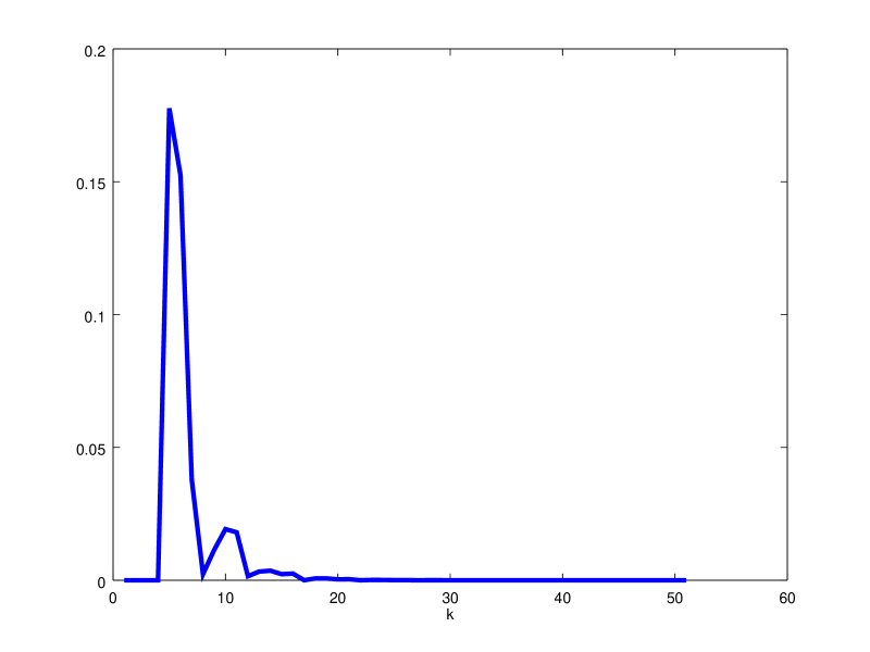
(a) $|h^{a*,K}(y)-1|$ as a function of $y=(k,k)$

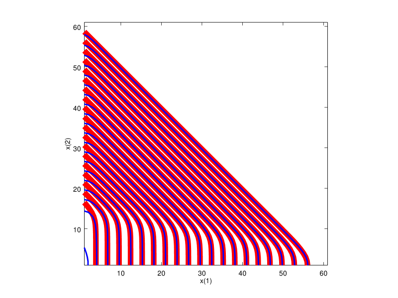
(b) Level curves of $-\frac{1}{n}\log h^{a,0}(T_{n}(x))$ and $-\frac{1}{n}\log P_{x}(\tau_{n}<\tau_{0})$, $n=60$

By Proposition 7.6

$$\left|\frac{P_{y}(\tau<\infty)-h^{a,0}(y)}{P_{y}(\tau<\infty)}\right|\leq c^{*}.$$

Theorem 6.1 now implies that $h^{a,K}(T_{n}(x_{n}))$ approximates $P_{x_{n}}(\tau_{n}<\tau_{0})$ with relative error bounded by $c^{*}=0.17764$ for $n$ large. Therefore, in improving our approximation from $h^{a,0}$ of (69) to $h^{a,3}$ by adding three $Y$-harmonic functions of the form $h_{\beta_{1}(\alpha_{1,j})}$ to the approximating basis, the relative error decreases from $c_{0}^{*}=0.3607$ to $c_{0}^{*}=0.17764$. Figure 6(b) shows the level curves of $-\frac{1}{n}\log h^{a,3}(T_{n}(x))$ and $-\frac{1}{n}\log P_{x}(\tau_{n}<\tau_{0})$ (the latter computed numerically via iteration of the harmonic equation satisfied by $P_{x}(\tau_{n}<\tau_{0})$) for $n=60$; the level curves overlap completely except along $\partial_{1}$, as suggested by our analysis.

To illustrate how the approximation error decreases when $K$ increases, let us repeat the computation above with $K=20$. The resulting maximum relative error turns out to be:

$$c^{*}=\max_{y\in\partial B}|h^{a*,20}(y)-1|=|h^{a*,20}((21,21))-1|=1.6211\times 10^{-3}.$$

The probability $P_{(4,0)}(\tau_{60}<\tau_{0})$, computed numerically, equals $4.6658\times 10^{-17}$, the best approximation of this quantity computed above is $h^{a,20}(56,0)=5.2\times 10^{-17}.$ The discrepancy arises from the proximity of $(4,0)$ to $\partial_{1}.$ As we move away from the $\partial_{1}$, these quantities get closer $P_{(10,0)}(\tau_{60}<\tau_{0})=3.3303\times 10^{-15}$, $h^{a,20}(50,0)=3.3358\times 10^{-15}$, compatible with the maximum relative error computed above. Figure 7 shows how approximation improves as $K$ increases:

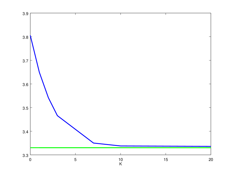
Figure 7:    $K\mapsto h^{a,K}(50,0)$ and $P_{(10,0)}(\tau_{60}<\tau_{0})$ (the flat line), drawn at $10^{-15}$ scale

8 Comparison with the tandem case

This section compares the analysis and results of the current work to those of [66] treating the approximation of the probability $P_{x}(\tau_{n}<\tau_{0})$ for the constrained random walk representing two tandem queues, which has the increments $(1,0)$, $(-1,1)$ and $(0,-1).$ The main idea is the same for both walks: i.e., approximation of $P_{x}(\tau_{n}<\tau_{0})$ by $P_{y}(\tau<\infty)$ and computing/ approximating the latter via harmonic functions constructed out of single and conjugate points on the characteristic surface. However, the assumptions, the results and the analysis manifest nontrivial differences. Let us begin with the assumptions:

Assumption $r^{2}/\rho_{2}<1$

In the tandem case $\beta_{1}(1)=\rho_{2}$ and the conjugate point of $(\rho_{2},1)$ is $(\rho_{2},\rho_{1})$, therefore, the stability assumption automatically implies $\bm{\alpha}(r,1)<1$. For the parallel case, $\bm{\alpha}(r,1)$ can indeed be greater than $1$ if $r$ and $\rho_{1}$ are close and $\rho_{2}$ is small; we therefore explicitly assume $r^{2}/\rho_{2}<1.$ This assumption appears in two places: 1) in the convergence analysis, in the derivation of the bound (18) and 2) in the computation of $P_{y}(\tau<\infty)$ in Section 7. We think that the use of the assumption $r^{2}/\rho_{2}<1$ in the first case can be removed without much change from the arguments of the present and earlier works; the details remain for future work. We think that the computation of $P_{y}(\tau<\infty)$ when $r^{2}/\rho_{2}>1$ presents genuine difficulties, the treatment of which also remains for future work. Next we point out the differences in results:

Region where $P_{y}(\tau<\infty)$ is a good approximation for $P_{x}(\tau_{n}<\tau_{0})$

That the tandem walk involves no jumps of the form $(-1,0)$ implies that $P_{T_{n}(x_{n})}(\tau<\infty)$ provides an approximation of $P_{x_{n}}(\tau_{n}<\tau_{0})$ with exponentially decaying relative error for all $x$ away from $0$; in contrast, the presence of the jump $(-1,0)$ in the parallel case, implies that the same approximation works only away from $\partial_{1}$ for the parallel walk case treated in the present work. This difference shows itself in the proofs of exponential decay of relative error, too, this is discussed below.

Explicit formula for $P_{y}(\tau<\infty)$

In the case of the tandem walk, the probability $P_{y}(\tau<\infty)$ can be explicitly represented as a linear combination of the harmonic functions $h_{\rho_{1}}$ and $h_{\rho_{2}}$ for all stable parameter values as long as $\mu_{1}\neq\mu_{2}$; in the parallel case this only happens when $r^{2}=\rho_{1}\rho_{2}$ (see Proposition 7.2). When $r^{2}\neq\rho_{1}\rho_{2}$, $h_{r}$ and $h_{\rho_{1}}$ can only provide an approximation of $P_{y}(\tau<\infty)$ with bounded relative error (Proposition 7.3). This relative error can be reduced by adding into the approximation further $\partial B$-determined $Y$-harmonic functions (Proposition 7.6 and subsection 7.1).

The changes in argument from the tandem walk to the parallel walk are as follows:

Analysis of $P_{x}(\tau_{n}<\tau_{0})$

In prior works [62, 28, 63, 65] the LD analysis of $P_{x}(\tau_{n}<\tau_{0})$ and similar quantities are based on sub and supersolutions of the limit HJB equation, similar to the analysis given in subsection 4.1. In the present work, a novelty is the use of explicit subharmonic functions (Proposition 4.2) of the constrained random walk $X$ in the proof of the upperbound Proposition 4.3.

Analysis of $P_{x}(\sigma_{1}<\tau_{n}<\tau_{0})$

The probability corresponding to $P_{x}(\sigma_{1}<\tau_{n}<\tau_{0})$ in the tandem case is $P_{x}(\sigma_{1}<\sigma_{1,2}<\tau_{n}<\tau_{0})$. For the proof of the exponential decay of the relative error, we need upperbound on these probabilities. Both papers develop these upperbound from subsolutions to a limit HJB equation. The subsolution consists of three pieces (one for each of the stopping times $\sigma_{1}$, $\sigma_{1,2}$ and $\tau_{n}$) for the tandem walk, and two pieces for the parallel walk (one for each of the times $\sigma_{1}$ and $\tau_{n}$). In the tandem case, the pieces of the subsolution are constructed from the subsolution for the probability $P_{x}(\tau_{n}<\tau_{0})$, whereas in the parallel case a new piece is introduced based on the gradient $r_{4}$ of (48).

Analysis of $P_{x}(\bar{\sigma}_{1}<\tau<\infty)$

The probability corresponding to $P_{x}(\bar{\sigma}_{1}<\tau<\infty)$ in the tandem case is $P_{x}(\bar{\sigma}_{1}<\bar{\sigma}_{1,2}<\tau<\infty)$. The special nature of the tandem walk allowed us to find upperbounds on this probability from the explicit formula we have for $P_{y}(\tau<\infty)$; this significantly simplified the analysis of the tandem walk case. For the parallel walk, we extended the analysis of $P_{x}(\sigma_{1}<\tau_{n}<\tau_{0})$, based on subsolutions, to $P_{x}(\bar{\sigma}_{1}<\tau<\infty)$. In this, the most significant novelty is the analysis given Section 3, where we prove the existence of $z>1$ such that ${\mathbb{E}}_{z}[z^{\tau}1_{\{\tau<\infty\}}]<\infty$. For this, we introduce what we call $Y-z$-harmonic functions and provide methods of construction of classes of them from points on $1/z$-level characteristic surfaces, which are generalizations of characteristic surfaces.

9 Conclusion

The probability $P_{y}(\tau<\infty)$ approximates $P_{x}(\tau_{n}<\tau_{0})$ well when $x$ is away from $\partial_{1}$; as noted in the previous section, this is in contrast to the tandem case, where the approximation is good away from the origin. How can one extend the approximation to the region along $\partial_{1}$? A natural idea, already pointed out in [65] is to repeat the same analysis, but this time taking the corner $(0,n)$ as the origin of the $Y$ process, i.e., to use the change of coordinate $y=T_{n}(x)=(x(1),n-x(2))$ to construct the $Y$ process. Numerical calculations indicate that the resulting approximation will be accurate (i.e., exponentially decaying relative error) along $\partial_{1}$ between the points $(0,n)$ and $(0,\lfloor(1-C_{4})n\rfloor)$ (see (28) for the definition of $C_{4}$). We believe that arguments and computations parallel to the ones given in the present work would imply these results; the details are left for future work. We think that the extension of the approximation to the region along the line segment between $(0,0)$ and $(0,\lfloor(1-c_{1})n\rfloor)$ requires further ideas and computations.

We expect the analysis linking $P_{x}(\tau_{n}<\tau_{0})$ to $P_{y}(\tau<\infty)$ when $\rho_{1}=\rho_{2}$ to be parallel to the analysis given in the current work. For the computation of $P_{y}(\tau<\infty)$, when $\rho_{1}=\rho_{2}$, the case $\lambda_{1}=\lambda_{2}$, $\mu_{1}=\mu_{2}$ appears to be particularly simple. In this case, upon taking limits in (58) one obtains

$$P_{y}(\tau<\infty)=r^{y(1)-y(2)}+(1-r)r^{y(1)}(y(1)-y(2)),$$

where $r=\rho_{1}=\rho_{2}$. A complete analysis of the computation of $P_{y}(\tau<\infty)$ when $\rho_{1}=\rho_{2}$ remains for future work.

In subsection 7.1, the computation of $P_{y}(\tau<\infty)$ when $r^{2}\neq\rho_{1}\rho_{2}$ proceeds as follows: 1) we first construct a candidate approximation $h^{a,K}=\Re(h^{a*,K})$ of $P_{y}(\tau<\infty)$ 2) we find an upperbound on the relative error of the approximation by finding the maximum of $|h^{a*,K}-1|$ on $\partial B.$ A natural question is the following: given a relative error bound, can we know apriori that an approximation having that maximum relative error can be constructed? If that is possible, how many $Y$-harmonic functions of the form given by Proposition 2.2 would we need? To answer these questions require a fine understanding of the functional analytic properties of the span of the $\partial B$-determined $Y$-harmonic functions given by Propositions 2.1 and 2.2. This appears to be a difficult problem because the functions given in these propositions don’t have simple geometric properties, such as the orthogonality of the Fourier basis in $L^{2}$. A study of this problem remains for future work.

The exact formula for $P_{y}(\tau<\infty)$ for the tandem case has a remarkable extension to $d$ dimensions; this is derived in [65] and is based on harmonic-systems, a concept defined in that work. We think that it is also possible, in the case of parallel queues, to obtain nontrivial harmonic systems in higher dimensions. A complete characterization of such systems and the question of under what conditions they would give a rich class of $Y$-harmonic functions to approximate $P_{y}(\tau<\infty)$ also remain challenging problems for future research.

References

- [1] Murat Alanyali and Bruce Hajek, On large deviations in load sharing networks, Annals of Applied Probability (1998), 67–97.
- [2] David Aldous, Probability approximations via the poisson clumping heuristic, vol. 77, Springer Science & Business Media, 2013.
- [3] Jayaram Anantharam, Philip Heidelberger, and Pantelis Tsoucas, Analysis of rare events in continuous time Markov chains via time reversal and fluid approximation, Tech Rep, IBM Research (1990).
- [4] Søren Asmussen, Applied probability and queues, vol. 51, Springer Science & Business Media, 2008.
- [5] Søren Asmussen and Peter Glynn, Stochastic simulation: Algorithms and analysis, vol. 57, Springer Science & Business Media, 2007.
- [6] Rami Atar and Paul Dupuis, Large deviations and queueing networks: methods for rate function identification, Stochastic processes and their applications 84 (1999), no. 2, 255–296.
- [7] J Blanchet, P. Glynn, and K. Leder, Efficient simulation of light-tailed sums: an old folk song sung to a faster new tune, Monte Carlo and Quasi-Monte Carlo Methods 2008 (2008), 227–258.
- [8] J. Blanchet, P. Glynn, and K. Leder, On lyapunov inequalities and subsolutions for efficient importance sampling, (2009), Preprint.
- [9] Jose Blanchet, Optimal sampling of overflow paths in jackson networks, Mathematics of Operations Research 38 (2013), no. 4, 698–719.
- [10] José Blanchet and Michel Mandjes, Rare event simulation for queues, Rare Event Simulation Using Monte Carlo Methods (2009), 87–124.
- [11] Pieter-Tjerk De Boer, Dirk P. Kroese, and Reuven Y. Rubenstein, A fast cross-entropy method for estimating buffer overflows in queueing networks, Management Science 50 (2004), 883–895.
- [12] Pieter-Tjerk De Boer and Victor F. Nicola, Adaptive state-dependent importance sampling simulation of Markovian queueing networks, European Transactions on Telecommunications 13 (2001), 303–315.
- [13] Aleksandr Alekseevich Borovkov and Anatolii Al’fredovich Mogul’skii, Large deviations for markov chains in the positive quadrant, Russian Mathematical Surveys 56 (2001), no. 5, 803–916.
- [14] Michelle Boué, Paul Dupuis, and Richard S. Ellis, Large deviations for small noise diffusions with discontinuous statistics, Probab. Theory Related Fields 116 (2000), no. 1, 125–149. MR MR1736592 (2001a:60032)
- [15] Cheng-Shang Chang, Philip Heidelberger, Sandeep Juneja, and Perwez Shahabuddin, Effective bandwith and fast simulation of ATM intree networks, Performance Evaluation 20 (1994), 45–66.
- [16] Jesse Collingwood, Robert D Foley, and David R McDonald, Networks with cascading overloads, Proceedings of the 6th International Conference on Queueing Theory and Network Applications, ACM, 2011, pp. 33–37.
- [17] Francis Comets, François Delarue, and René Schott, Distributed algorithms in an ergodic markovian environment, Random Structures & Algorithms 30 (2007), no. 1-2, 131–167.
- [18] , Large deviations analysis for distributed algorithms in an ergodic markovian environment, Applied Mathematics and Optimization 60 (2009), no. 3, 341–396.
- [19] Michael A. Crane and Donald L. Iglehart, Simulating stable stochastic systems, i: General multiserver queues, Journal of the Association for Computing Machinery 21 (1974), no. 1, 103–113.
- [20] Jim G Dai, Masakiyo Miyazawa, et al., Reflecting brownian motion in two dimensions: Exact asymptotics for the stationary distribution, Stochastic Systems 1 (2011), no. 1, 146–208.
- [21] Pieter-Tjerk de Boer, Analysis of state-independent importance-sampling measures for the two-node tandem queue, ACM Transactions on Modeling and Computer Simulation (TOMACS) 16 (2006), no. 3, 225–250.
- [22] Thomas Dean and Paul Dupuis, Splitting for rare event simulation: A large deviation approach to design and analysis, Stochastic processes and their applications 119 (2009), no. 2, 562–587.
- [23] Antonius Ton Dieker and Michel Mandjes, On asymptotically efficient simulation of large deviation probabilities, Advances in applied probability (2005), 539–552.
- [24] Paul Dupuis and Richard Ellis, A weak convergence approach to the theory of large deviations, John Wiley & Sons, New York, 1997.
- [25] Paul Dupuis and Richard S Ellis, The large deviation principle for a general class of queueing systems. i, Transactions of the American Mathematical Society 347 (1995), no. 8, 2689–2751.
- [26] Paul Dupuis and Hitoshi Ishii, On Lipschitz continuity of the solution mapping to the Skorokhod problem, with applications, Stochastics Stochastics Rep. 35 (1991), no. 1, 31–62. MR MR1110990 (93e:60110)
- [27] Paul Dupuis, Kevin Leder, and Hui Wang, Importance sampling for sums of random variables with regularly varying tails, ACM Trans. Model. Comput. Simul. 17 (2007), no. 3, 14.
- [28] Paul Dupuis, Ali Devin Sezer, and Hui Wang, Dynamic importance sampling for queueing networks, Annals of Applied Probability 17 (2007), no. 4, 1306–1346.
- [29] Paul Dupuis and Hui Wang, Importance sampling, large deviations and differential games, Stochastics and Stochastic Reports 76 (2004), no. 6, 481–508.
- [30] , Importance sampling for Jackson networks, Queueing Systems 62 (2009), 113–157.
- [31] Rick Durrett, Probability: theory and examples, 4th edition, Cambridge university press, 2010.
- [32] Philippe Flajolet, The evolution of two stacks in bounded space and random walks in a triangle, Springer, 1986.
- [33] Robert D Foley and David R McDonald, Constructing a harmonic function for an irreducible nonnegative matrix with convergence parameter r¿ 1, Bulletin of the London Mathematical Society (2012), bdr115.
- [34] Robert D Foley, David R McDonald, et al., Large deviations of a modified jackson network: Stability and rough asymptotics, The Annals of Applied Probability 15 (2005), no. 1B, 519–541.
- [35] Michael R Frater, Tava M Lennon, and Brian DO Anderson, Optimally efficient estimation of the statistics of rare events in queueing networks, IEEE Transactions on Automatic Control 36 (1991), no. 12, 1395–1405.
- [36] Nadine Guillotin-Plantard and René Schott, Dynamic random walks: Theory and applications, Elsevier, 2006.
- [37] Irina Ignatiouk-Robert, Large deviations of jackson networks, Annals of Applied Probability (2000), 962–1001.
- [38] Irina Ignatiouk-Robert and Christophe Loree, Martin boundary of a killed random walk on a quadrant, The Annals of Probability (2010), 1106–1142.
- [39] IA Ignatyuk, Vadim Aleksandrovich Malyshev, and VV Scherbakov, Boundary effects in large deviation problems, Russian Mathematical Surveys 49 (1994), no. 2, 41–99.
- [40] Sandeep Juneja and Victor Nicola, Efficient simulation of buffer overflow probabilities in Jackson networks with feedback, ACM Transcations on Modeling and Computer Simulation 15 (2005), 281–315.
- [41] Sandeep Juneja and Perwez Shahabuddin, Rare-event simulation techniques: an introduction and recent advances, Handbooks in operations research and management science 13 (2006), 291–350.
- [42] Donald Ervin Knuth, Art of computer programming volume 1: Fundamental algorithms, Addison-Wesley Publishing Company, 1972.
- [43] Masahiro Kobayashi and Masakiyo Miyazawa, Revisiting the tail asymptotics of the double qbd process: refinement and complete solutions for the coordinate and diagonal directions, Matrix-Analytic Methods in Stochastic Models, Springer, 2013, pp. 145–185.
- [44] Dirk P. Kroese and Victor Nicola, Efficient simulation of Jackson networks, ACM Transactions on Modeling and Computer Simulation 12 (2002), 119–141.
- [45] IA Kurkova and VA Malyshev, Martin boundary and elliptic curves, Markov Process. Related Fields 4 (1998), no. 2, 203–272.
- [46] Guy Louchard and Rene Schott, Probabilistic analysis of some distributed algorithms, Random Structures & Algorithms 2 (1991), no. 2, 151–186.
- [47] Guy Louchard, René Schott, Michael Tolley, and P Zimmermann, Random walks, heat equation and distributed algorithms, Journal of Computational and Applied Mathematics 53 (1994), no. 2, 243–274.
- [48] Robert S Maier, Colliding stacks: A large deviations analysis, Random Structures & Algorithms 2 (1991), no. 4, 379–420.
- [49] , Large fluctuations in stochastically perturbed nonlinear systems: Applications in computing, arXiv preprint chao-dyn/9305009 (1993).
- [50] Kurt Majewski and Kavita Ramanan, How large queue lengths build up in a jackson network, preprint (2008).
- [51] DR McDonald, Asymptotics of first passage times for random walk in an orthant, Annals of Applied Probability (1999), 110–145.
- [52] Denis Miretskiy, Werner Scheinhardt, and Michael Robertus Hendrikus Mandjes, State-dependent importance sampling for a jackson tandem network, (2008).
- [53] Masakiyo Miyazawa, Tail decay rates in double qbd processes and related reflected random walks, Mathematics of Operations Research 34 (2009), no. 3, 547–575.
- [54] , Light tail asymptotics in multidimensional reflecting processes for queueing networks, Top 19 (2011), no. 2, 233–299.
- [55] Peter Ney and Esa Nummelin, Markov additive processes i. eigenvalue properties and limit theorems, The Annals of Probability (1987), 561–592.
- [56] Victor Nicola and Tatiana Zaburnenko, Efficient importance sampling heuristics for the simulation of population overflow in jackson networks, ACM Transactions on Modeling and Computer Simulation (TOMACS) 17 (2007), no. 2, 10.
- [57] Shyam Parekh and Jean Walrand, A quick simulation method for excessive backlogs in networks of queues, IEEE Transactions on Automatic Control 34 (1989), no. 1, 54–66.
- [58] R.S. Randhawa and S. Juneja, Combining importance sampling and temporal difference control variates to simulate markov chains, ACM Transactions on Modeling and Computer Simulation 14 (2004), no. 1, 1–30.
- [59] Ad Ridder, Importance sampling algorithms for first passage time probabilities in the infinite server queue, European Journal of Operational Research 199 (2009), no. 1, 176–186.
- [60] Gerardo Rubino and Bruno Tuffin, Rare event simulation using monte carlo methods, John Wiley & Sons, 2009.
- [61] Leila Setayeshgar and Hui Wang, Efficient importance sampling schemes for a feed-forward network, ACM Transactions on Modeling and Computer Simulation (TOMACS) 23 (2013), no. 4, 21.
- [62] Ali Devin Sezer, Dynamic importance sampling for queueing networks, ph.d. thesis, Brown University Division of Applied Mathematics, 2005.
- [63] Ali Devin Sezer, Importance sampling for a markov modulated queuing network, Stochastic Processes and their Applications 119 (2009), no. 2, 491–517.
- [64] , Asymptotically optimal importance sampling for Jackson networks with a tree topology, Queueing Systems 64 (2010), no. 2, 103–117, Longer (2007) version available at http://arxiv.org/abs/0708.3260.
- [65] , Exit probabilities and balayage of constrained random walks, https://arxiv.org/abs/1506.08674 (2015).
- [66] , Approximation of excessive backlog probabilities of two tandem queues, https://arxiv.org/abs/1801.04674 (2018).
- [67] Adam Shwartz and Alan Weiss, Large deviations for performance analysis, Stochastic Modeling Series, Chapman & Hall, London, 1995, Queues, communications, and computing, With an appendix by Robert J. Vanderbei. MR MR1335456 (96i:60029)
- [68] Andrew C Yao, An analysis of a memory allocation scheme for implementing stacks, SIAM Journal on Computing 10 (1981), no. 2, 398–403.