Signal and Noise Statistics Oblivious Orthogonal Matching Pursuit

Sreejith Kallummil โ€ƒโ€ƒ Sheetal Kalyani
Abstract

Orthogonal matching pursuit (OMP) is a widely used algorithm for recovering sparse high dimensional vectors in linear regression models. The optimal performance of OMP requires a priori knowledge of either the sparsity of regression vector or noise statistics. Both these statistics are rarely known a priori and are very difficult to estimate. In this paper, we present a novel technique called residual ratio thresholding (RRT) to operate OMP without any a priori knowledge of sparsity and noise statistics and establish finite sample and large sample support recovery guarantees for the same. Both analytical results and numerical simulations in real and synthetic data sets indicate that RRT has a performance comparable to OMP with a priori knowledge of sparsity and noise statistics.

High dimensional regression, sparsity

1 Introduction

This article deals with the estimation of the regression vector ๐œทโˆˆโ„p๐œทsuperscriptโ„๐‘\bm{\beta}\in\mathbb{R}^{p} in the linear regression model ๐ฒ=๐—โ€‹๐œท+๐ฐ๐ฒ๐—๐œท๐ฐ{\bf y}={\bf X}\bm{\beta}+{\bf w}, where ๐—โˆˆโ„nร—p๐—superscriptโ„๐‘›๐‘{\bf X}\in\mathbb{R}^{n\times p} is a known design matrix with unit Euclidean norm columns, ๐ฐ๐ฐ{\bf w} is the noise vector and ๐ฒ๐ฒ{\bf y} is the observation vector. Throughout this article, we assume that the entries of the noise ๐ฐ๐ฐ{\bf w} are independent, zero mean and Gaussian distributed with variance ฯƒ2superscript๐œŽ2\sigma^{2}. We consider the high dimensional and sample starved scenario of n<p๐‘›๐‘n<p or nโ‰ชpmuch-less-than๐‘›๐‘n\ll p where classical techniques like ordinary least squares (OLS) are no longer applicable. This problem of estimating high dimensional vectors in sample starved scenarios is ill-posed even in the absence of noise unless strong structural assumptions are made on ๐—๐—{\bf X} and ๐œท๐œท\bm{\beta}. A widely used and practically valid assumption is sparsity. The vector ๐œทโˆˆโ„p๐œทsuperscriptโ„๐‘\bm{\beta}\in\mathbb{R}^{p} is sparse if the support of ๐œท๐œท\bm{\beta} given by ๐’ฎ=sโ€‹uโ€‹pโ€‹pโ€‹(๐œท)={k:๐œทkโ‰ 0}๐’ฎ๐‘ ๐‘ข๐‘๐‘๐œทconditional-set๐‘˜subscript๐œท๐‘˜0\mathcal{S}=supp(\bm{\beta})=\{k:\bm{\beta}_{k}\neq 0\} has cardinality k0=cโ€‹aโ€‹rโ€‹dโ€‹(๐’ฎ)โ‰ชpsubscript๐‘˜0๐‘๐‘Ž๐‘Ÿ๐‘‘๐’ฎmuch-less-than๐‘k_{0}=card(\mathcal{S})\ll p.

A number of algorithms like least absolute shrinkage and selection operator (LASSO)(Tropp, 2006; Tibshirani, 1996), Dantzig selector (DS)(Candes & Tao, 2007), subspace pursuit (SP)(Dai & Milenkovic, 2009), OMP (Pati etย al., 1993; Mallat & Zhang, 1993; Tropp, 2004; Cai & Wang, 2011), elastic net (Zou & Hastie, 2005) etc. are proposed to efficiently estimate ๐œท๐œท\bm{\beta}. Tuning the hyper parameters of aforementioned algorithms to achieve optimal performance require a priori knowledge of signal parameters like sparsity k0subscript๐‘˜0k_{0} or noise statistics like ฯƒ2superscript๐œŽ2\sigma^{2} etc. Unfortunately, these parameters are rarely known a priori. To the best of our knowledge, no computationally efficient technique to estimate k0subscript๐‘˜0k_{0} is reported in open literature. However, limited success on the estimation of ฯƒ2superscript๐œŽ2\sigma^{2} has been reported in literature (Dicker, 2014; Fan etย al., 2012; Dicker & Erdogdu, 2016; Bayati etย al., 2013). However, the performance of these ฯƒ2superscript๐œŽ2\sigma^{2} estimates when used for tuning hyper parameters in LASSO, DS, OMP etc. are largely unknown. Generalised techniques for hyper parameter selection like cross validation (CV)(Arlot etย al., 2010), re-sampling (Meinshausen & Bรผhlmann, 2010) etc. are computationally challenging. Further, CV is reported to have poor variable selection behaviour(Chichignoud etย al., 2016; Arlot etย al., 2010). Indeed, algorithms that are oblivious to signal and noise statistics are also proposed in literature. This include algorithms inspired or related to LASSO like square root LASSO(Belloni etย al., 2011), AVโˆž (Chichignoud etย al., 2016), approximate message passing (Mousavi etย al., 2013; Bayati etย al., 2013) etc. and ridge regression inspired techniques like least squares adaptive thresholding (LAT), ridge adaptive thresholding (RAT)(Wang etย al., 2016) etc. However, most of existing signal and noise statistics oblivious sparse recovery techniques have only large sample performance guarantees. Further, many of these techniques assume that design matrix ๐—๐—{\bf X} is sampled from a random ensemble, a condition which is rarely satisfied in practice.

1.1 Contributions of this paper

This article present a novel technique called residual ratio thresholding (RRT) for finding a โ€œgoodโ€ estimate of support ๐’ฎ๐’ฎ\mathcal{S} from the data dependent/adaptive sequence of supports generated by OMP. RRT is analytically shown to accomplish exact support recovery, (i.e., identifying ๐’ฎ๐’ฎ\mathcal{S}) under the same finite sample and deterministic constraints on ๐—๐—{\bf X} like restricted isometry constants (RIC) or mutual coherence required by OMP with a priori knowledge of k0subscript๐‘˜0k_{0} or ฯƒ2superscript๐œŽ2\sigma^{2}. However, the signal to noise ratio (SNR=โ€–๐—โ€‹๐œทโ€–22/nโ€‹ฯƒ2superscriptsubscriptnorm๐—๐œท22๐‘›superscript๐œŽ2{\|{\bf X}\bm{\beta}\|_{2}^{2}}/{n\sigma^{2}}) required for support recovery using RRT is slightly higher than that of OMP with a priori knowledge of k0subscript๐‘˜0k_{0} or ฯƒ2superscript๐œŽ2\sigma^{2}. This extra SNR requirement is shown to decrease with the increase in sample size n๐‘›n. RRT and OMP with a priori knowledge of k0subscript๐‘˜0k_{0} or ฯƒ2superscript๐œŽ2\sigma^{2} are shown to be equivalent as nโ†’โˆžโ†’๐‘›n\rightarrow\infty in terms of the SNR required for support recovery. RRT involves a tuning parameter ฮฑ๐›ผ\alpha that can be set independent of ambient SNR or noise statistics. The hyper parameter ฮฑ๐›ผ\alpha in RRT have an interesting semantic interpretation of being the high SNR upper bound on support recovery error. Also RRT is asymptotically tuning free in the sense that a very wide range of ฮฑ๐›ผ\alpha deliver similar performances as nโ†’โˆžโ†’๐‘›n\rightarrow\infty. Numerical simulations indicate that RRT can deliver a highly competitive performance when compared to OMP having a priori knowledge of k0subscript๐‘˜0k_{0} or ฯƒ2superscript๐œŽ2\sigma^{2}, OMP with k0subscript๐‘˜0k_{0} estimated using CV and the recently proposed LAT algorithm. Further, RRT also delivered a highly competitive performance when applied to identify outliers in real data sets, an increasingly popular application of sparse estimation algorithms(Mitra etย al., 2010, 2013).

The remainder of this article is organised as follows. In section 2 we discuss OMP algorithm. RRT algorithm is presented in Section 3. Section 4 presents theoretical performance guarantees for RRT. Section 5 presents numerical simulation results. All the proofs are provided in the supplementary material.

1.2 Notations used

โ€–๐ฑโ€–q=(โˆ‘k=1p|๐ฑk|q)1qsubscriptnorm๐ฑ๐‘žsuperscriptsuperscriptsubscript๐‘˜1๐‘superscriptsubscript๐ฑ๐‘˜๐‘ž1๐‘ž\|{\bf x}\|_{q}=\left(\sum\limits_{k=1}^{p}|{\bf x}_{k}|^{q}\right)^{\frac{1}{q}} is the lqsubscript๐‘™๐‘žl_{q} norm of ๐ฑโˆˆโ„p๐ฑsuperscriptโ„๐‘{\bf x}\in\mathbb{R}^{p}. ๐ŸŽnsubscript0๐‘›{\bf 0}_{n} is the nร—1๐‘›1n\times 1 zero vector and ๐ˆnsubscript๐ˆ๐‘›{\bf I}_{n} is the nร—n๐‘›๐‘›n\times n identity matrix. sโ€‹pโ€‹aโ€‹nโ€‹(๐—)๐‘ ๐‘๐‘Ž๐‘›๐—span({\bf X}) is the column space of ๐—๐—{\bf X}. ๐—โ€ =(๐—Tโ€‹๐—)โˆ’1โ€‹๐—Tsuperscript๐—โ€ superscriptsuperscript๐—๐‘‡๐—1superscript๐—๐‘‡{\bf X}^{\dagger}=({\bf X}^{T}{\bf X})^{-1}{\bf X}^{T} is the Moore-Penrose pseudo inverse of ๐—๐—{\bf X}. ๐—๐’ฅsubscript๐—๐’ฅ{\bf X}_{\mathcal{J}} denotes the sub-matrix of ๐—๐—{\bf X} formed using the columns indexed by ๐’ฅ๐’ฅ\mathcal{J}. ๐’ฉโ€‹(๐ฎ,๐‚)๐’ฉ๐ฎ๐‚\mathcal{N}({\bf u},{\bf C}) represents a Gaussian random vector (R.V) with mean ๐ฎ๐ฎ{\bf u} and covariance matrix ๐‚๐‚{\bf C}. ๐”นโ€‹(a,b)๐”น๐‘Ž๐‘\mathbb{B}(a,b) denotes a Beta R.V with parameters a๐‘Ža and b๐‘b. ๐šโˆผ๐›similar-to๐š๐›{\bf a}\sim{\bf b} implies that ๐š๐š{\bf a} and ๐›๐›{\bf b} are identically distributed. [p]delimited-[]๐‘[p] represents the floor operator. ฯ•italic-ฯ•\phi represents the null set. For any two sets ๐’ฅ1subscript๐’ฅ1\mathcal{J}_{1} and ๐’ฅ2subscript๐’ฅ2\mathcal{J}_{2}, ๐’ฅ1/๐’ฅ2subscript๐’ฅ1subscript๐’ฅ2\mathcal{J}_{1}/\mathcal{J}_{2} denotes the set difference. ๐šโ€‹โ†’๐‘ƒโ€‹๐›๐š๐‘ƒโ†’๐›{\bf a}\overset{P}{\rightarrow}{\bf b} represents the convergence of R.V ๐š๐š{\bf a} to R.V ๐›๐›{\bf b} in probability.

2 Orthogonal matching pursuit (OMP)

OMP (Algorithm 1) starts with a null support estimate and in each iteration it adds that column index to the current support which is the most correlated with the previous residual ๐ซkโˆ’1superscript๐ซ๐‘˜1{\bf r}^{k-1}, i.e., tk=argโกmax๐‘—โ€‹|๐—jTโ€‹๐ซkโˆ’1|subscript๐‘ก๐‘˜๐‘—superscriptsubscript๐—๐‘—๐‘‡superscript๐ซ๐‘˜1t_{k}=\underset{j}{\arg\max}|{\bf X}_{j}^{T}{\bf r}^{k-1}|. Then a LS estimate of ๐œท๐œท\bm{\beta} restricted to the current support ๐’ฎoโ€‹mโ€‹pksubscriptsuperscript๐’ฎ๐‘˜๐‘œ๐‘š๐‘\mathcal{S}^{k}_{omp} is computed as an intermediate estimate of ๐œท๐œท\bm{\beta} and this estimate is used to update the residual. Note that ๐ksubscript๐๐‘˜{\bf P}_{k} in Algorithm 1 refers to ๐—๐’ฎoโ€‹mโ€‹pkโ€‹๐—๐’ฎoโ€‹mโ€‹pkโ€ subscript๐—subscriptsuperscript๐’ฎ๐‘˜๐‘œ๐‘š๐‘superscriptsubscript๐—subscriptsuperscript๐’ฎ๐‘˜๐‘œ๐‘š๐‘โ€ {\bf X}_{\mathcal{S}^{k}_{omp}}{\bf X}_{\mathcal{S}^{k}_{omp}}^{\dagger}, the projection matrix onto sโ€‹pโ€‹aโ€‹nโ€‹(๐—๐’ฎoโ€‹mโ€‹pk)๐‘ ๐‘๐‘Ž๐‘›subscript๐—subscriptsuperscript๐’ฎ๐‘˜๐‘œ๐‘š๐‘span({\bf X}_{\mathcal{S}^{k}_{omp}}). Since the residual ๐ซksuperscript๐ซ๐‘˜{\bf r}^{k} is orthogonal to sโ€‹pโ€‹aโ€‹nโ€‹(๐—๐’ฎoโ€‹mโ€‹pk)๐‘ ๐‘๐‘Ž๐‘›subscript๐—subscriptsuperscript๐’ฎ๐‘˜๐‘œ๐‘š๐‘span({\bf X}_{\mathcal{S}^{k}_{omp}}), ๐—jTโ€‹๐ซk=0superscriptsubscript๐—๐‘—๐‘‡superscript๐ซ๐‘˜0{\bf X}_{j}^{T}{\bf r}^{k}=0 for all jโˆˆ๐’ฎoโ€‹mโ€‹pk๐‘—subscriptsuperscript๐’ฎ๐‘˜๐‘œ๐‘š๐‘j\in\mathcal{S}^{k}_{omp}. Consequently, tk+1โˆ‰๐’ฎoโ€‹mโ€‹pksubscript๐‘ก๐‘˜1subscriptsuperscript๐’ฎ๐‘˜๐‘œ๐‘š๐‘t_{k+1}\notin{\mathcal{S}^{k}_{omp}}, i.e., the same index will not be selected in two different iterations. Hence, ๐’ฎoโ€‹mโ€‹pk+1โŠƒ๐’ฎoโ€‹mโ€‹pksubscriptsuperscript๐’ฎ๐‘˜๐‘œ๐‘š๐‘subscriptsuperscript๐’ฎ๐‘˜1๐‘œ๐‘š๐‘\mathcal{S}^{k+1}_{omp}\supset\mathcal{S}^{k}_{omp}, i.e. the support sequence is monotonically increasing. The monotonicity of ๐’ฎoโ€‹mโ€‹pksubscriptsuperscript๐’ฎ๐‘˜๐‘œ๐‘š๐‘\mathcal{S}^{k}_{omp} in turn implies that the residual norm โ€–๐ซkโ€–2subscriptnormsuperscript๐ซ๐‘˜2\|{\bf r}^{k}\|_{2} is a non increasing function of k๐‘˜k, i.e, โ€–๐ซk+1โ€–2โ‰คโ€–๐ซkโ€–2subscriptnormsuperscript๐ซ๐‘˜12subscriptnormsuperscript๐ซ๐‘˜2\|{\bf r}^{k+1}\|_{2}\leq\|{\bf r}^{k}\|_{2}.

Algorithm 1 Orthogonal matching pursuit
ย ย Input: Observation ๐ฒ๐ฒ{\bf y}, matrix ๐—๐—{\bf X}
ย ย Initialize ๐’ฎ0oโ€‹mโ€‹p=ฯ•superscriptsubscript๐’ฎ0๐‘œ๐‘š๐‘italic-ฯ•\mathcal{S}_{0}^{omp}=\phi. k=1๐‘˜1k=1 and residual ๐ซ0=๐ฒsuperscript๐ซ0๐ฒ{\bf r}^{0}={\bf y}
ย ย repeat
ย ย ย ย ย Identify the next column tk=argโกmax๐‘—โ€‹|๐—jTโ€‹๐ซkโˆ’1|subscript๐‘ก๐‘˜๐‘—superscriptsubscript๐—๐‘—๐‘‡superscript๐ซ๐‘˜1t_{k}=\underset{j}{\arg\max}|{\bf X}_{j}^{T}{\bf r}^{k-1}|
ย ย ย ย ย Expand current support ๐’ฎoโ€‹mโ€‹pk=๐’ฎoโ€‹mโ€‹pkโˆ’1โˆชtksubscriptsuperscript๐’ฎ๐‘˜๐‘œ๐‘š๐‘subscriptsuperscript๐’ฎ๐‘˜1๐‘œ๐‘š๐‘subscript๐‘ก๐‘˜\mathcal{S}^{k}_{omp}=\mathcal{S}^{k-1}_{omp}\cup t_{k}
ย ย ย ย ย Restricted LS estimate: ๐œท^๐’ฎoโ€‹mโ€‹pk=๐—๐’ฎoโ€‹mโ€‹pkโ€ โ€‹๐ฒsubscript^๐œทsubscriptsuperscript๐’ฎ๐‘˜๐‘œ๐‘š๐‘superscriptsubscript๐—subscriptsuperscript๐’ฎ๐‘˜๐‘œ๐‘š๐‘โ€ ๐ฒ\hat{\bm{\beta}}_{\mathcal{S}^{k}_{omp}}={\bf X}_{\mathcal{S}^{k}_{omp}}^{\dagger}{\bf y}.
ย ย ย ย ย ย ย ย ย ย ย ย ย ย ย ย ย ย ย ย ย ย ย ย ย ย ย ย ย ย ย ย ย ย ย ย ย ย ย ย ย ย ย ย ย ๐œท^{1,โ€ฆ,p}/๐’ฎoโ€‹mโ€‹pk=๐ŸŽpโˆ’ksubscript^๐œท1โ€ฆ๐‘subscriptsuperscript๐’ฎ๐‘˜๐‘œ๐‘š๐‘subscript0๐‘๐‘˜\hat{\bm{\beta}}_{\{1,\dotsc,p\}/\mathcal{S}^{k}_{omp}}={\bf 0}_{p-k}.
ย ย ย ย ย Update residual: ๐ซk=๐ฒโˆ’๐—โ€‹๐œท^=(๐ˆnโˆ’๐k)โ€‹๐ฒsuperscript๐ซ๐‘˜๐ฒ๐—^๐œทsubscript๐ˆ๐‘›subscript๐๐‘˜๐ฒ{\bf r}^{k}={\bf y}-{\bf X}\hat{\bm{\beta}}=({\bf I}_{n}-{\bf P}_{k}){\bf y}.
ย ย ย ย ย Increment kโ†k+1โ†๐‘˜๐‘˜1k\leftarrow k+1.
ย ย untilย stopping condition (SC) is true
ย ย Output: Support estimate S^=๐’ฎoโ€‹mโ€‹pk^๐‘†superscriptsubscript๐’ฎ๐‘œ๐‘š๐‘๐‘˜\hat{S}=\mathcal{S}_{omp}^{k}. Vector estimate ๐œท^^๐œท\hat{\bm{\beta}}

Most of the theoretical properties of OMP are derived assuming a priori knowledge of true sparsity level k0subscript๐‘˜0k_{0} in which case OMP stops after exactly k0subscript๐‘˜0k_{0} iterations(Tropp, 2004; Wang, 2015). When k0subscript๐‘˜0k_{0} is not known, one has to rely on stopping conditions (SC) based on the properties of the residual ๐ซksuperscript๐ซ๐‘˜{\bf r}^{k} as k๐‘˜k varies. For example, one can stop OMP iterations once the residual power is too low compared to the expected noise power. Mathematically, when the noise ๐ฐ๐ฐ{\bf w} is l2subscript๐‘™2l_{2} bounded, i.e., โ€–๐ฐโ€–2โ‰คฯต2subscriptnorm๐ฐ2subscriptitalic-ฯต2\|{\bf w}\|_{2}\leq\epsilon_{2} for some a priori known ฯต2subscriptitalic-ฯต2\epsilon_{2}, then OMP can be stopped if โ€–๐ซkโ€–2โ‰คฯต2subscriptnormsuperscript๐ซ๐‘˜2subscriptitalic-ฯต2\|{\bf r}^{k}\|_{2}\leq\epsilon_{2}. For a Gaussian noise vector ๐ฐโˆผ๐’ฉโ€‹(๐ŸŽn,ฯƒ2โ€‹๐ˆn)similar-to๐ฐ๐’ฉsubscript0๐‘›superscript๐œŽ2subscript๐ˆ๐‘›{\bf w}\sim\mathcal{N}({\bf 0}_{n},\sigma^{2}{\bf I}_{n}), ฯตฯƒ=ฯƒโ€‹n+2โ€‹nโ€‹logโก(n)subscriptitalic-ฯต๐œŽ๐œŽ๐‘›2๐‘›๐‘›\epsilon_{\sigma}=\sigma\sqrt{n+2\sqrt{n\log(n)}} satisfies(Cai & Wang, 2011)

โ„™โ€‹(โ€–๐ฐโ€–2โ‰คฯตฯƒ)โ‰ฅ1โˆ’1n,โ„™subscriptnorm๐ฐ2subscriptitalic-ฯต๐œŽ11๐‘›\mathbb{P}(\|{\bf w}\|_{2}\leq\epsilon_{\sigma})\geq 1-\frac{1}{n}, (1)

i.e., Gaussian noise is l2subscript๐‘™2l_{2} bounded with a very high probability. Consequently, one can stop OMP iterations in Gaussian noise once โ€–๐ซkโ€–2โ‰คฯตฯƒsubscriptnormsuperscript๐ซ๐‘˜2subscriptitalic-ฯต๐œŽ\|{\bf r}^{k}\|_{2}\leq\epsilon_{\sigma}.

A number of deterministic recovery guarantees are proposed for OMP. Among these guarantees the conditions based on RIC are the most popular. RIC of order j๐‘—j denoted by ฮดjsubscript๐›ฟ๐‘—\delta_{j} is defined as the smallest value of ฮด๐›ฟ\delta such that

(1โˆ’ฮด)โ€‹โ€–๐›โ€–22โ‰คโ€–๐—๐›โ€–22โ‰ค(1+ฮด)โ€‹โ€–๐›โ€–221๐›ฟsuperscriptsubscriptnorm๐›22superscriptsubscriptnorm๐—๐›221๐›ฟsuperscriptsubscriptnorm๐›22(1-\delta)\|{\bf b}\|_{2}^{2}\leq\|{\bf X}{\bf b}\|_{2}^{2}\leq(1+\delta)\|{\bf b}\|_{2}^{2} (2)

hold true for all ๐›โˆˆโ„p๐›superscriptโ„๐‘{\bf b}\in\mathbb{R}^{p} with โ€–๐›โ€–0=cโ€‹aโ€‹rโ€‹dโ€‹(sโ€‹uโ€‹pโ€‹pโ€‹(๐›))โ‰คjsubscriptnorm๐›0๐‘๐‘Ž๐‘Ÿ๐‘‘๐‘ ๐‘ข๐‘๐‘๐›๐‘—\|{\bf b}\|_{0}=card(supp({\bf b}))\leq j. A smaller value of ฮดjsubscript๐›ฟ๐‘—\delta_{j} implies that ๐—๐—{\bf X} act as a near orthogonal matrix for all j๐‘—j sparse vectors ๐›๐›{\bf b}. Such a situation is ideal for the recovery of a j๐‘—j-sparse vector ๐›๐›{\bf b} using any sparse recovery technique. The latest RIC based support recovery guarantee using OMP is given in Lemma 1(Liu etย al., 2017).

Lemma 1.

OMP with k0subscript๐‘˜0k_{0} iterations or SC โ€–๐ซkโ€–2โ‰คโ€–๐ฐโ€–2subscriptnormsuperscript๐ซ๐‘˜2subscriptnorm๐ฐ2\|{\bf r}^{k}\|_{2}\leq\|{\bf w}\|_{2} can recover any k0subscript๐‘˜0k_{0} sparse vector ๐›ƒ๐›ƒ\bm{\beta} provided that ฮดk0+1<1/k0+1subscript๐›ฟsubscript๐‘˜011subscript๐‘˜01\delta_{k_{0}+1}<{1}/{\sqrt{k_{0}+1}} and โ€–๐ฐโ€–2โ‰คฯตoโ€‹mโ€‹p=๐›ƒmโ€‹iโ€‹nโ€‹1โˆ’ฮดk0+1โ€‹[1โˆ’k0+1โ€‹ฮดk0+11+1โˆ’ฮดk0+12โˆ’k0+1โ€‹ฮดk0+1]subscriptnorm๐ฐ2subscriptitalic-ฯต๐‘œ๐‘š๐‘subscript๐›ƒ๐‘š๐‘–๐‘›1subscript๐›ฟsubscript๐‘˜01delimited-[]1subscript๐‘˜01subscript๐›ฟsubscript๐‘˜0111superscriptsubscript๐›ฟsubscript๐‘˜012subscript๐‘˜01subscript๐›ฟsubscript๐‘˜01\|{\bf w}\|_{2}\leq\epsilon_{omp}=\bm{\beta}_{min}\sqrt{1-\delta_{k_{0}+1}}\left[\dfrac{1-\sqrt{k_{0}+1}\delta_{k_{0}+1}}{1+\sqrt{1-\delta_{k_{0}+1}^{2}}-\sqrt{k_{0}+1}\delta_{k_{0}+1}}\right].

Since โ„™โ€‹(โ€–๐ฐโ€–2<ฯตฯƒ)โ‰ฅ1โˆ’1/nโ„™subscriptnorm๐ฐ2subscriptitalic-ฯต๐œŽ11๐‘›\mathbb{P}(\|{\bf w}\|_{2}<\epsilon_{\sigma})\geq 1-1/n when ๐ฐโˆผ๐’ฉโ€‹(๐ŸŽn,ฯƒ2โ€‹๐ˆn)similar-to๐ฐ๐’ฉsubscript0๐‘›superscript๐œŽ2subscript๐ˆ๐‘›{\bf w}\sim\mathcal{N}({\bf 0}_{n},\sigma^{2}{\bf I}_{n}), it follows from Lemma 1 that OMP with k0subscript๐‘˜0k_{0} iterations or SC โ€–๐ซkโ€–2โ‰คฯตฯƒsubscriptnormsuperscript๐ซ๐‘˜2subscriptitalic-ฯต๐œŽ\|{\bf r}^{k}\|_{2}\leq\epsilon_{\sigma} can recover any k0subscript๐‘˜0k_{0}-sparse vector ๐œท๐œท\bm{\beta} with probability greater than 1โˆ’1/n11๐‘›1-1/n provided that ฮดk0+1<1/k0+1subscript๐›ฟsubscript๐‘˜011subscript๐‘˜01\delta_{k_{0}+1}<{1}/{\sqrt{k_{0}+1}} and ฯตฯƒโ‰คฯตoโ€‹mโ€‹psubscriptitalic-ฯต๐œŽsubscriptitalic-ฯต๐‘œ๐‘š๐‘\epsilon_{\sigma}\leq\epsilon_{omp}. Lemma 1 implies that OMP with a priori knowledge of k0subscript๐‘˜0k_{0} or ฯƒ2superscript๐œŽ2\sigma^{2} can recover support ๐’ฎ๐’ฎ\mathcal{S} once the matrix satisfies the regularity condition ฮดk0+1<1/k0+1subscript๐›ฟsubscript๐‘˜011subscript๐‘˜01\delta_{k_{0}+1}<{1}/{\sqrt{k_{0}+1}} and the SNR is high. It is also known that this RIC condition is worst case necessary. Consequently, Lemma 1 is one of the best deterministic guarantee for OMP available in literature. Note that the mutual incoherence condition given by ฮผ๐—=maxjโ‰ kโ€‹|๐—jTโ€‹๐—k|<1/(2โ€‹k0โˆ’1)subscript๐œ‡๐—๐‘—๐‘˜superscriptsubscript๐—๐‘—๐‘‡subscript๐—๐‘˜12subscript๐‘˜01\mu_{\bf X}=\underset{j\neq k}{\max}|{\bf X}_{j}^{T}{\bf X}_{k}|<1/(2k_{0}-1) also ensures exact support recovery at high SNR. Note that the a priori knowledge of k0subscript๐‘˜0k_{0} or ฯƒ2superscript๐œŽ2\sigma^{2} required to materialise the recovery guarantees in Lemma 1 are not available in practical problems. Further, k0subscript๐‘˜0k_{0} and ฯƒ2superscript๐œŽ2\sigma^{2} are very difficult to estimate. This motivates the proposed RRT algorithm which does not require a priori knowledge of k0subscript๐‘˜0k_{0} or ฯƒ2superscript๐œŽ2\sigma^{2}.

3 Residual ratio thresholding (RRT)

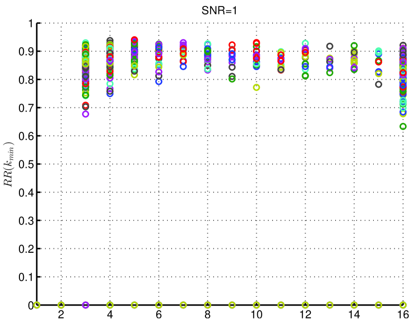
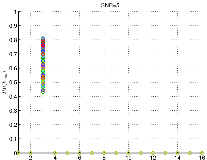
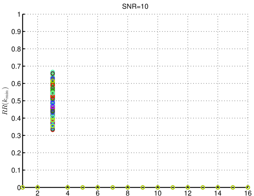
RRT is a novel signal and noise statistics oblivious technique to estimate the support ๐’ฎ๐’ฎ\mathcal{S} based on the behaviour of the residual ratio statistic Rโ€‹Rโ€‹(k)=โ€–๐ซkโ€–2/โ€–๐ซkโˆ’1โ€–2๐‘…๐‘…๐‘˜subscriptnormsuperscript๐ซ๐‘˜2subscriptnormsuperscript๐ซ๐‘˜12RR(k)={\|{\bf r}^{k}\|_{2}}/{\|{\bf r}^{k-1}\|_{2}} as k๐‘˜k increases from k=1๐‘˜1k=1 to a predefined value k=kmโ€‹aโ€‹x>k0๐‘˜subscript๐‘˜๐‘š๐‘Ž๐‘ฅsubscript๐‘˜0k=k_{max}>k_{0}. As aforementioned, identifying the support using the behaviour of โ€–๐ซkโ€–2subscriptnormsuperscript๐ซ๐‘˜2\|{\bf r}^{k}\|_{2} requires a priori knowledge of ฯƒ2superscript๐œŽ2\sigma^{2}. However, as we will show in this section, support detection using Rโ€‹Rโ€‹(k)๐‘…๐‘…๐‘˜RR(k) does not require a priori knowledge of ฯƒ2superscript๐œŽ2\sigma^{2}. Since the residual norms are non negative and non increasing, Rโ€‹Rโ€‹(k)๐‘…๐‘…๐‘˜RR(k) always satisfy 0โ‰คRโ€‹Rโ€‹(k)โ‰ค10๐‘…๐‘…๐‘˜10\leq RR(k)\leq 1.

3.1 Minimal Superset and implications

Consider running kmโ€‹aโ€‹x>k0subscript๐‘˜๐‘š๐‘Ž๐‘ฅsubscript๐‘˜0k_{max}>k_{0} iterations of OMP and let {๐’ฎoโ€‹mโ€‹pk}k=1kโ€‹mโ€‹aโ€‹xsuperscriptsubscriptsubscriptsuperscript๐’ฎ๐‘˜๐‘œ๐‘š๐‘๐‘˜1๐‘˜๐‘š๐‘Ž๐‘ฅ\{\mathcal{S}^{k}_{omp}\}_{k=1}^{kmax} be the support sequence generated by OMP. Recall that ๐’ฎoโ€‹mโ€‹pksubscriptsuperscript๐’ฎ๐‘˜๐‘œ๐‘š๐‘\mathcal{S}^{k}_{omp} is monotonically increasing.

Definition 1:- The minimal superset in the OMP support sequence {๐’ฎoโ€‹mโ€‹pk}k=1kโ€‹mโ€‹aโ€‹xsuperscriptsubscriptsubscriptsuperscript๐’ฎ๐‘˜๐‘œ๐‘š๐‘๐‘˜1๐‘˜๐‘š๐‘Ž๐‘ฅ\{\mathcal{S}^{k}_{omp}\}_{k=1}^{kmax} is given by ๐’ฎoโ€‹mโ€‹pkmโ€‹iโ€‹nsuperscriptsubscript๐’ฎ๐‘œ๐‘š๐‘subscript๐‘˜๐‘š๐‘–๐‘›\mathcal{S}_{omp}^{k_{min}}, where kmโ€‹iโ€‹n=minโก({k:๐’ฎโŠ†๐’ฎoโ€‹mโ€‹pk})subscript๐‘˜๐‘š๐‘–๐‘›conditional-set๐‘˜๐’ฎsubscriptsuperscript๐’ฎ๐‘˜๐‘œ๐‘š๐‘k_{min}=\min(\{k:\mathcal{S}\subseteq\mathcal{S}^{k}_{omp}\}). When the set {k:๐’ฎโŠ†๐’ฎoโ€‹mโ€‹pk}=ฯ•conditional-set๐‘˜๐’ฎsubscriptsuperscript๐’ฎ๐‘˜๐‘œ๐‘š๐‘italic-ฯ•\{k:\mathcal{S}\subseteq\mathcal{S}^{k}_{omp}\}=\phi, we set kmโ€‹iโ€‹n=โˆžsubscript๐‘˜๐‘š๐‘–๐‘›k_{min}=\infty and ๐’ฎoโ€‹mโ€‹pkmโ€‹iโ€‹n=ฯ•subscriptsuperscript๐’ฎsubscript๐‘˜๐‘š๐‘–๐‘›๐‘œ๐‘š๐‘italic-ฯ•\mathcal{S}^{k_{min}}_{omp}=\phi.

In words, minimal superset is the smallest superset of support ๐’ฎ๐’ฎ\mathcal{S} present in a particular realization of the support estimate sequence {๐’ฎoโ€‹mโ€‹pk}k=1kโ€‹mโ€‹aโ€‹xsuperscriptsubscriptsubscriptsuperscript๐’ฎ๐‘˜๐‘œ๐‘š๐‘๐‘˜1๐‘˜๐‘š๐‘Ž๐‘ฅ\{\mathcal{S}^{k}_{omp}\}_{k=1}^{kmax}. Note that both kmโ€‹iโ€‹nsubscript๐‘˜๐‘š๐‘–๐‘›k_{min} and ๐’ฎoโ€‹mโ€‹pkmโ€‹iโ€‹nsuperscriptsubscript๐’ฎ๐‘œ๐‘š๐‘subscript๐‘˜๐‘š๐‘–๐‘›\mathcal{S}_{omp}^{k_{min}} are unobservable random variables. Since cโ€‹aโ€‹rโ€‹dโ€‹(๐’ฎoโ€‹mโ€‹pk)=k๐‘๐‘Ž๐‘Ÿ๐‘‘subscriptsuperscript๐’ฎ๐‘˜๐‘œ๐‘š๐‘๐‘˜card(\mathcal{S}^{k}_{omp})=k, ๐’ฎoโ€‹mโ€‹pksubscriptsuperscript๐’ฎ๐‘˜๐‘œ๐‘š๐‘\mathcal{S}^{k}_{omp} for k<k0๐‘˜subscript๐‘˜0k<k_{0} cannot satisfy ๐’ฎโŠ†๐’ฎoโ€‹mโ€‹pk๐’ฎsubscriptsuperscript๐’ฎ๐‘˜๐‘œ๐‘š๐‘\mathcal{S}\subseteq\mathcal{S}^{k}_{omp} and hence kmโ€‹iโ€‹nโ‰ฅk0subscript๐‘˜๐‘š๐‘–๐‘›subscript๐‘˜0k_{min}\geq k_{0}. Further, the monotonicity of ๐’ฎoโ€‹mโ€‹pksubscriptsuperscript๐’ฎ๐‘˜๐‘œ๐‘š๐‘\mathcal{S}^{k}_{omp} implies that ๐’ฎโŠ‚๐’ฎoโ€‹mโ€‹pk๐’ฎsubscriptsuperscript๐’ฎ๐‘˜๐‘œ๐‘š๐‘\mathcal{S}\subset\mathcal{S}^{k}_{omp} for all kโ‰ฅkmโ€‹iโ€‹n๐‘˜subscript๐‘˜๐‘š๐‘–๐‘›k\geq k_{min}.
Case 1:- When kmโ€‹iโ€‹n=k0subscript๐‘˜๐‘š๐‘–๐‘›subscript๐‘˜0k_{min}=k_{0}, then ๐’ฎoโ€‹mโ€‹pk0=๐’ฎsubscriptsuperscript๐’ฎsubscript๐‘˜0๐‘œ๐‘š๐‘๐’ฎ\mathcal{S}^{k_{0}}_{omp}=\mathcal{S} and ๐’ฎoโ€‹mโ€‹pkโŠƒ๐’ฎ๐’ฎsubscriptsuperscript๐’ฎ๐‘˜๐‘œ๐‘š๐‘\mathcal{S}^{k}_{omp}\supset\mathcal{S} for kโ‰ฅk0๐‘˜subscript๐‘˜0k\geq k_{0}, i.e., ๐’ฎ๐’ฎ\mathcal{S} is present in the solution path. Further, when kmโ€‹iโ€‹n=k0subscript๐‘˜๐‘š๐‘–๐‘›subscript๐‘˜0k_{min}=k_{0}, it is true that ๐’ฎoโ€‹mโ€‹pkโŠ†๐’ฎsuperscriptsubscript๐’ฎ๐‘œ๐‘š๐‘๐‘˜๐’ฎ\mathcal{S}_{omp}^{k}\subseteq\mathcal{S} for kโ‰คk0๐‘˜subscript๐‘˜0k\leq k_{0}.
Case 2:- When k0<kmโ€‹iโ€‹nโ‰คkmโ€‹aโ€‹xsubscript๐‘˜0subscript๐‘˜๐‘š๐‘–๐‘›subscript๐‘˜๐‘š๐‘Ž๐‘ฅk_{0}<k_{min}\leq k_{max}, then ๐’ฎoโ€‹mโ€‹pkโ‰ ๐’ฎsubscriptsuperscript๐’ฎ๐‘˜๐‘œ๐‘š๐‘๐’ฎ\mathcal{S}^{k}_{omp}\neq\mathcal{S} for all k๐‘˜k and ๐’ฎkoโ€‹mโ€‹pโŠƒ๐’ฎ๐’ฎsuperscriptsubscript๐’ฎ๐‘˜๐‘œ๐‘š๐‘\mathcal{S}_{k}^{omp}\supset\mathcal{S} for kโ‰ฅkmโ€‹iโ€‹n๐‘˜subscript๐‘˜๐‘š๐‘–๐‘›k\geq k_{min}, i.e., ๐’ฎ๐’ฎ\mathcal{S} is not present in the solution path. However, a superset of ๐’ฎ๐’ฎ\mathcal{S} is present.
Case 3:- When kmโ€‹iโ€‹n=โˆžsubscript๐‘˜๐‘š๐‘–๐‘›k_{min}=\infty, then ๐’ฎoโ€‹mโ€‹pkโŠ‰๐’ฎnot-superset-of-or-equalssubscriptsuperscript๐’ฎ๐‘˜๐‘œ๐‘š๐‘๐’ฎ\mathcal{S}^{k}_{omp}\not\supseteq\mathcal{S} for all k๐‘˜k, i.e., neither ๐’ฎ๐’ฎ\mathcal{S} nor a superset of ๐’ฎ๐’ฎ\mathcal{S} is present in {๐’ฎoโ€‹mโ€‹pk}k=1kโ€‹mโ€‹aโ€‹xsuperscriptsubscriptsubscriptsuperscript๐’ฎ๐‘˜๐‘œ๐‘š๐‘๐‘˜1๐‘˜๐‘š๐‘Ž๐‘ฅ\{\mathcal{S}^{k}_{omp}\}_{k=1}^{kmax}.
To summarize, exact support recovery using any OMP based scheme including the signal and noise statistics aware schemes is possible only if kmโ€‹iโ€‹n=k0subscript๐‘˜๐‘š๐‘–๐‘›subscript๐‘˜0k_{min}=k_{0}. Whenever kmโ€‹iโ€‹n>k0subscript๐‘˜๐‘š๐‘–๐‘›subscript๐‘˜0k_{min}>k_{0}, it is possible to estimate true support ๐’ฎ๐’ฎ\mathcal{S} without having any false negatives. However, one then has to suffer from false positives. When kmโ€‹iโ€‹n=โˆžsubscript๐‘˜๐‘š๐‘–๐‘›k_{min}=\infty, any support in {๐’ฎoโ€‹mโ€‹pk}k=1kโ€‹mโ€‹aโ€‹xsuperscriptsubscriptsubscriptsuperscript๐’ฎ๐‘˜๐‘œ๐‘š๐‘๐‘˜1๐‘˜๐‘š๐‘Ž๐‘ฅ\{\mathcal{S}^{k}_{omp}\}_{k=1}^{kmax} has to suffer from false negatives and all supports ๐’ฎoโ€‹mโ€‹pksubscriptsuperscript๐’ฎ๐‘˜๐‘œ๐‘š๐‘\mathcal{S}^{k}_{omp} for k>k0โˆ’1๐‘˜subscript๐‘˜01k>k_{0}-1 has to suffer from false positives also. Note that the matrix and SNR conditions required for exact support recovery in Lemma 1 automatically implies that kmโ€‹iโ€‹n=k0subscript๐‘˜๐‘š๐‘–๐‘›subscript๐‘˜0k_{min}=k_{0}. We formulate the proposed RRT scheme assuming that kmโ€‹iโ€‹n=k0subscript๐‘˜๐‘š๐‘–๐‘›subscript๐‘˜0k_{min}=k_{0}.

3.2 Behaviour of Rโ€‹Rโ€‹(k0)๐‘…๐‘…subscript๐‘˜0RR(k_{0})

Next we consider the behaviour of residual ratio statistic at the k0subscript๐‘˜0k_{0} iteration, i.e., Rโ€‹Rโ€‹(k0)=โ€–๐ซk0โ€–2/โ€–๐ซk0โˆ’1โ€–2๐‘…๐‘…subscript๐‘˜0subscriptnormsuperscript๐ซsubscript๐‘˜02subscriptnormsuperscript๐ซsubscript๐‘˜012RR(k_{0})={\|{\bf r}^{k_{0}}\|_{2}}/{\|{\bf r}^{k_{0}-1}\|_{2}} under the assumption that โ€–๐ฐโ€–2โ‰คฯตoโ€‹mโ€‹psubscriptnorm๐ฐ2subscriptitalic-ฯต๐‘œ๐‘š๐‘\|{\bf w}\|_{2}\leq\epsilon_{omp} and ฮดk0+1<1/k0+1subscript๐›ฟsubscript๐‘˜011subscript๐‘˜01\delta_{k_{0}+1}<1/\sqrt{k_{0}+1} which ensures kmโ€‹iโ€‹n=k0subscript๐‘˜๐‘š๐‘–๐‘›subscript๐‘˜0k_{min}=k_{0} and ๐’ฎoโ€‹mโ€‹pkโŠ†๐’ฎsuperscriptsubscript๐’ฎ๐‘œ๐‘š๐‘๐‘˜๐’ฎ\mathcal{S}_{omp}^{k}\subseteq\mathcal{S} for all kโ‰คk0๐‘˜subscript๐‘˜0k\leq k_{0}. Since ๐—โ€‹๐œท=๐—๐’ฎโ€‹๐œท๐’ฎโˆˆsโ€‹pโ€‹aโ€‹nโ€‹(๐—๐’ฎ)๐—๐œทsubscript๐—๐’ฎsubscript๐œท๐’ฎ๐‘ ๐‘๐‘Ž๐‘›subscript๐—๐’ฎ{\bf X}\bm{\beta}={\bf X}_{\mathcal{S}}\bm{\beta}_{\mathcal{S}}\in span({\bf X}_{\mathcal{S}}), (๐ˆnโˆ’๐k)โ€‹๐—โ€‹๐œทโ‰ ๐ŸŽnsubscript๐ˆ๐‘›subscript๐๐‘˜๐—๐œทsubscript0๐‘›({\bf I}_{n}-{\bf P}_{k}){\bf X}\bm{\beta}\neq{\bf 0}_{n} if ๐’ฎโŠˆ๐’ฎoโ€‹mโ€‹pknot-subset-of-or-equals๐’ฎsubscriptsuperscript๐’ฎ๐‘˜๐‘œ๐‘š๐‘\mathcal{S}\not\subseteq\mathcal{S}^{k}_{omp} and (๐ˆnโˆ’๐k)โ€‹๐—โ€‹๐œท=๐ŸŽnsubscript๐ˆ๐‘›subscript๐๐‘˜๐—๐œทsubscript0๐‘›({\bf I}_{n}-{\bf P}_{k}){\bf X}\bm{\beta}={\bf 0}_{n} if ๐’ฎโŠ†๐’ฎoโ€‹mโ€‹pk๐’ฎsubscriptsuperscript๐’ฎ๐‘˜๐‘œ๐‘š๐‘\mathcal{S}\subseteq\mathcal{S}^{k}_{omp}. This along with the monotonicity of ๐’ฎoโ€‹mโ€‹pksubscriptsuperscript๐’ฎ๐‘˜๐‘œ๐‘š๐‘\mathcal{S}^{k}_{omp} implies the following. (๐ˆnโˆ’๐k)โ€‹๐—โ€‹๐œทโ‰ ๐ŸŽnsubscript๐ˆ๐‘›subscript๐๐‘˜๐—๐œทsubscript0๐‘›({\bf I}_{n}-{\bf P}_{k}){\bf X\bm{\beta}}\neq{\bf 0}_{n} for k<kmโ€‹iโ€‹n=k0๐‘˜subscript๐‘˜๐‘š๐‘–๐‘›subscript๐‘˜0k<k_{min}=k_{0} and (๐ˆnโˆ’๐k)โ€‹๐—โ€‹๐œท=๐ŸŽnsubscript๐ˆ๐‘›subscript๐๐‘˜๐—๐œทsubscript0๐‘›({\bf I}_{n}-{\bf P}_{k}){\bf X\bm{\beta}}={\bf 0}_{n} for kโ‰ฅkmโ€‹iโ€‹n=k0๐‘˜subscript๐‘˜๐‘š๐‘–๐‘›subscript๐‘˜0k\geq k_{min}=k_{0}. Thus ๐ซk=(๐ˆnโˆ’๐k)โ€‹๐ฒ=(๐ˆnโˆ’๐k)โ€‹๐—๐’ฎโ€‹๐œท๐’ฎ+(๐ˆnโˆ’๐k)โ€‹๐ฐsuperscript๐ซ๐‘˜subscript๐ˆ๐‘›subscript๐๐‘˜๐ฒsubscript๐ˆ๐‘›subscript๐๐‘˜subscript๐—๐’ฎsubscript๐œท๐’ฎsubscript๐ˆ๐‘›subscript๐๐‘˜๐ฐ{\bf r}^{k}=({\bf I}_{n}-{\bf P}_{k}){\bf y}=({\bf I}_{n}-{\bf P}_{k}){\bf X}_{\mathcal{S}}{\bm{\beta}_{\mathcal{S}}}+({\bf I}_{n}-{\bf P}_{k}){\bf w} for k<kmโ€‹iโ€‹n=k0๐‘˜subscript๐‘˜๐‘š๐‘–๐‘›subscript๐‘˜0k<k_{min}=k_{0}, whereas, ๐ซk=(๐ˆnโˆ’๐k)โ€‹๐ฐsuperscript๐ซ๐‘˜subscript๐ˆ๐‘›subscript๐๐‘˜๐ฐ{\bf r}^{k}=({\bf I}_{n}-{\bf P}_{k}){\bf w} for kโ‰ฅkmโ€‹iโ€‹n=k0๐‘˜subscript๐‘˜๐‘š๐‘–๐‘›subscript๐‘˜0k\geq k_{min}=k_{0}. Consequently, at k=k0๐‘˜subscript๐‘˜0k=k_{0}, the numerator โ€–๐ซk0โ€–2subscriptnormsuperscript๐ซsubscript๐‘˜02\|{\bf r}^{k_{0}}\|_{2} of Rโ€‹Rโ€‹(k0)๐‘…๐‘…subscript๐‘˜0RR(k_{0}) contains contribution only from the noise term โ€–(๐ˆnโˆ’๐k0)โ€‹๐ฐโ€–2subscriptnormsubscript๐ˆ๐‘›subscript๐subscript๐‘˜0๐ฐ2\|({\bf I}_{n}-{\bf P}_{k_{0}}){\bf w}\|_{2}, whereas, the denominator โ€–๐ซk0โˆ’1โ€–2subscriptnormsuperscript๐ซsubscript๐‘˜012\|{\bf r}^{k_{0}-1}\|_{2} in Rโ€‹Rโ€‹(k0)๐‘…๐‘…subscript๐‘˜0RR(k_{0}) contain contributions from both the signal term i.e., (๐ˆnโˆ’๐k)โ€‹๐—๐’ฎโ€‹๐œท๐’ฎsubscript๐ˆ๐‘›subscript๐๐‘˜subscript๐—๐’ฎsubscript๐œท๐’ฎ({\bf I}_{n}-{\bf P}_{k}){\bf X}_{\mathcal{S}}{\bm{\beta}_{\mathcal{S}}} and the noise term (๐ˆnโˆ’๐k)โ€‹๐ฐsubscript๐ˆ๐‘›subscript๐๐‘˜๐ฐ({\bf I}_{n}-{\bf P}_{k}){\bf w}. This behaviour of Rโ€‹Rโ€‹(k0)๐‘…๐‘…subscript๐‘˜0RR(k_{0}) along with the fact that โ€–๐ฐโ€–2โ€‹โ†’๐‘ƒโ€‹0subscriptnorm๐ฐ2๐‘ƒโ†’0\|{\bf w}\|_{2}\overset{P}{\rightarrow}0 as ฯƒ2โ†’0โ†’superscript๐œŽ20\sigma^{2}\rightarrow 0 implies the following theorem.

Theorem 1.

Assume that the matrix ๐—๐—{\bf X} satisfies the RIC constraint ฮดk0+1<1/k0+1subscript๐›ฟsubscript๐‘˜011subscript๐‘˜01\delta_{k_{0}+1}<{1}/{\sqrt{k_{0}+1}} and kmโ€‹aโ€‹x>k0subscript๐‘˜๐‘š๐‘Ž๐‘ฅsubscript๐‘˜0k_{max}>k_{0}. Then
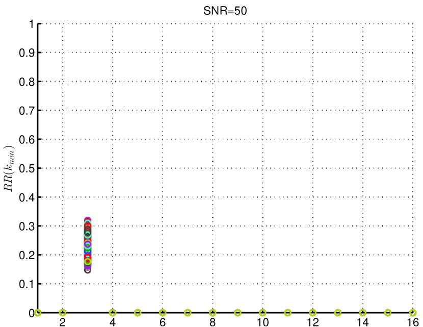
a). Rโ€‹Rโ€‹(kmโ€‹iโ€‹n)โ€‹โ†’๐‘ƒโ€‹0๐‘…๐‘…subscript๐‘˜๐‘š๐‘–๐‘›๐‘ƒโ†’0RR(k_{min})\overset{P}{\rightarrow}0 as ฯƒ2โ†’0โ†’superscript๐œŽ20\sigma^{2}\rightarrow 0.
b). limฯƒ2โ†’0โ€‹โ„™โ€‹(kmโ€‹iโ€‹n=k0)=1โ†’superscript๐œŽ20โ„™subscript๐‘˜๐‘š๐‘–๐‘›subscript๐‘˜01\underset{\sigma^{2}\rightarrow 0}{\lim}\mathbb{P}(k_{min}=k_{0})=1.

3.3 Behaviour of Rโ€‹Rโ€‹(k)๐‘…๐‘…๐‘˜RR(k) for k>kmโ€‹iโ€‹n๐‘˜subscript๐‘˜๐‘š๐‘–๐‘›k>k_{min}

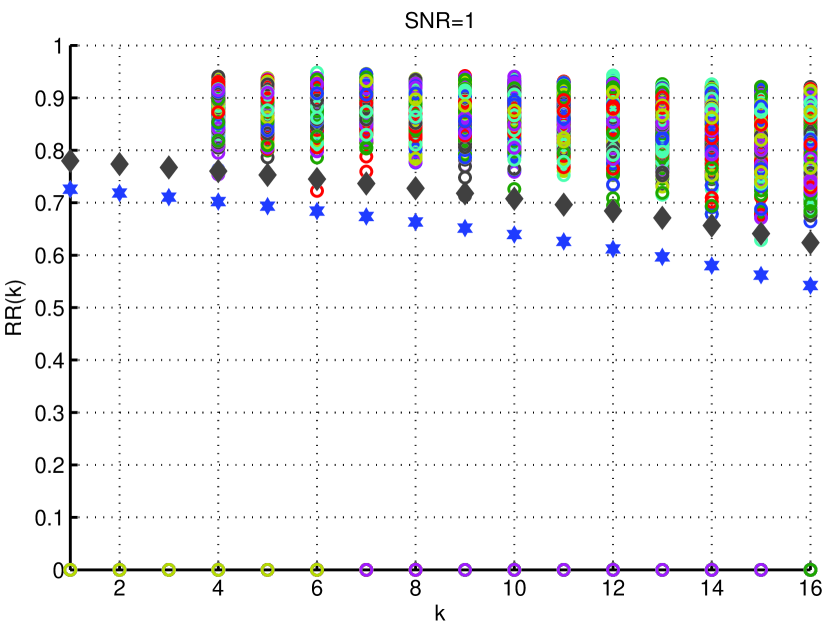
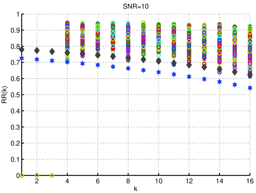
Next we discuss the behaviour of Rโ€‹Rโ€‹(k)๐‘…๐‘…๐‘˜RR(k) for k>kmโ€‹iโ€‹n๐‘˜subscript๐‘˜๐‘š๐‘–๐‘›k>k_{min}. By the definition of kmโ€‹iโ€‹nsubscript๐‘˜๐‘š๐‘–๐‘›k_{min} we have ๐’ฎโŠ†๐’ฎoโ€‹mโ€‹pk๐’ฎsubscriptsuperscript๐’ฎ๐‘˜๐‘œ๐‘š๐‘\mathcal{S}\subseteq\mathcal{S}^{k}_{omp} which implies that ๐ซk=(๐ˆnโˆ’๐k)โ€‹๐ฐsuperscript๐ซ๐‘˜subscript๐ˆ๐‘›subscript๐๐‘˜๐ฐ{\bf r}^{k}=({\bf I}_{n}-{\bf P}_{k}){\bf w} for kโ‰ฅkmโ€‹iโ€‹n๐‘˜subscript๐‘˜๐‘š๐‘–๐‘›k\geq k_{min}. The absence of signal terms in numerator and the denominator of Rโ€‹Rโ€‹(k)=โ€–(๐ˆnโˆ’๐k)โ€‹๐ฐโ€–2โ€–(๐ˆnโˆ’๐kโˆ’1)โ€‹๐ฐโ€–2๐‘…๐‘…๐‘˜subscriptnormsubscript๐ˆ๐‘›subscript๐๐‘˜๐ฐ2subscriptnormsubscript๐ˆ๐‘›subscript๐๐‘˜1๐ฐ2RR(k)=\frac{\|({\bf I}_{n}-{\bf P}_{k}){\bf w}\|_{2}}{\|({\bf I}_{n}-{\bf P}_{k-1}){\bf w}\|_{2}} for k>kmโ€‹iโ€‹n๐‘˜subscript๐‘˜๐‘š๐‘–๐‘›k>k_{min} implies that even when โ€–๐ฐโ€–2โ†’0โ†’subscriptnorm๐ฐ20\|{\bf w}\|_{2}\rightarrow 0 or ฯƒ2โ†’0โ†’superscript๐œŽ20\sigma^{2}\rightarrow 0, Rโ€‹Rโ€‹(k)๐‘…๐‘…๐‘˜RR(k) for k>kmโ€‹iโ€‹n๐‘˜subscript๐‘˜๐‘š๐‘–๐‘›k>k_{min} does not converge to zero. This behaviour of Rโ€‹Rโ€‹(k)๐‘…๐‘…๐‘˜RR(k) for k>kmโ€‹iโ€‹n๐‘˜subscript๐‘˜๐‘š๐‘–๐‘›k>k_{min} is captured in Theorem 2 where we provide explicit ฯƒ2superscript๐œŽ2\sigma^{2} or SNR independent lower bounds on Rโ€‹Rโ€‹(k)๐‘…๐‘…๐‘˜RR(k) for k>kmโ€‹iโ€‹n๐‘˜subscript๐‘˜๐‘š๐‘–๐‘›k>k_{min}.

Theorem 2.

Let Fa,bโ€‹(x)subscript๐น๐‘Ž๐‘๐‘ฅF_{a,b}(x) denotes the cumulative distribution function of a ๐”นโ€‹(a,b)๐”น๐‘Ž๐‘\mathbb{B}(a,b) random variable. Then โˆ€ฯƒ2>0for-allsuperscript๐œŽ20\forall\sigma^{2}>0, ฮ“Rโ€‹Rโ€‹Tฮฑโ€‹(k)=Fnโˆ’k2,0.5โˆ’1โ€‹(ฮฑkmโ€‹aโ€‹xโ€‹(pโˆ’k+1))superscriptsubscriptฮ“๐‘…๐‘…๐‘‡๐›ผ๐‘˜superscriptsubscript๐น๐‘›๐‘˜20.51๐›ผsubscript๐‘˜๐‘š๐‘Ž๐‘ฅ๐‘๐‘˜1\Gamma_{RRT}^{\alpha}(k)=\sqrt{F_{\frac{n-k}{2},0.5}^{-1}\left(\dfrac{\alpha}{k_{max}(p-k+1)}\right)} satisfies

โ„™โ€‹(Rโ€‹Rโ€‹(k)>ฮ“Rโ€‹Rโ€‹Tฮฑโ€‹(k),โˆ€k>kmโ€‹iโ€‹n)โ‰ฅ1โˆ’ฮฑ.โ„™formulae-sequence๐‘…๐‘…๐‘˜superscriptsubscriptฮ“๐‘…๐‘…๐‘‡๐›ผ๐‘˜for-all๐‘˜subscript๐‘˜๐‘š๐‘–๐‘›1๐›ผ\mathbb{P}(RR(k)>\Gamma_{RRT}^{\alpha}(k),\forall k>k_{min})\geq 1-\alpha. (3)

Theorem 2 states that the residual ratio statistic Rโ€‹Rโ€‹(k)๐‘…๐‘…๐‘˜RR(k) for k>kmโ€‹iโ€‹n๐‘˜subscript๐‘˜๐‘š๐‘–๐‘›k>k_{min} is lower bounded by the deterministic sequence {ฮ“Rโ€‹Rโ€‹Tฮฑโ€‹(k)}k=kmโ€‹iโ€‹n+1kmโ€‹aโ€‹xsuperscriptsubscriptsuperscriptsubscriptฮ“๐‘…๐‘…๐‘‡๐›ผ๐‘˜๐‘˜subscript๐‘˜๐‘š๐‘–๐‘›1subscript๐‘˜๐‘š๐‘Ž๐‘ฅ\{\Gamma_{RRT}^{\alpha}(k)\}_{k=k_{min}+1}^{k_{max}} with a high probability (for small values of ฮฑ๐›ผ\alpha). Please note that kmโ€‹iโ€‹nsubscript๐‘˜๐‘š๐‘–๐‘›k_{min} is itself a R.V. Note that the sequence ฮ“Rโ€‹Rโ€‹Tฮฑโ€‹(k)superscriptsubscriptฮ“๐‘…๐‘…๐‘‡๐›ผ๐‘˜\Gamma_{RRT}^{\alpha}(k) is dependent only on the matrix dimensions n๐‘›n and p๐‘p. Further, Theorem 2 does not make any assumptions on the noise variance ฯƒ2superscript๐œŽ2\sigma^{2} or the design matrix ๐—๐—{\bf X}. Theorem 2 is extremely non trivial considering the fact that the support estimate sequence {๐’ฎoโ€‹mโ€‹pk}k=1kmโ€‹aโ€‹xsuperscriptsubscriptsuperscriptsubscript๐’ฎ๐‘œ๐‘š๐‘๐‘˜๐‘˜1subscript๐‘˜๐‘š๐‘Ž๐‘ฅ\{\mathcal{S}_{omp}^{k}\}_{k=1}^{k_{max}} produced by OMP is adaptive and data dependent.

Lemma 2.

The following important properties of ฮ“Rโ€‹Rโ€‹Tฮฑโ€‹(k)superscriptsubscriptฮ“๐‘…๐‘…๐‘‡๐›ผ๐‘˜\Gamma_{RRT}^{\alpha}(k) are direct consequences of the monotonicity of CDF and the fact that a Beta R.V take values only in [0,1]01[0,1].
1). ฮ“Rโ€‹Rโ€‹Tฮฑโ€‹(k)superscriptsubscriptฮ“๐‘…๐‘…๐‘‡๐›ผ๐‘˜\Gamma_{RRT}^{\alpha}(k) is defined only in the interval ฮฑโˆˆ[0,kmโ€‹aโ€‹xโ€‹(pโˆ’k+1)]๐›ผ0subscript๐‘˜๐‘š๐‘Ž๐‘ฅ๐‘๐‘˜1\alpha\in[0,k_{max}(p-k+1)].
2). 0โ‰คฮ“Rโ€‹Rโ€‹Tฮฑโ€‹(k)โ‰ค10superscriptsubscriptฮ“๐‘…๐‘…๐‘‡๐›ผ๐‘˜10\leq\Gamma_{RRT}^{\alpha}(k)\leq 1.
3). ฮ“Rโ€‹Rโ€‹Tฮฑโ€‹(k)superscriptsubscriptฮ“๐‘…๐‘…๐‘‡๐›ผ๐‘˜\Gamma_{RRT}^{\alpha}(k) is a monotonically increasing function of ฮฑ๐›ผ\alpha.
4). ฮ“Rโ€‹Rโ€‹Tฮฑโ€‹(k)=0superscriptsubscriptฮ“๐‘…๐‘…๐‘‡๐›ผ๐‘˜0\Gamma_{RRT}^{\alpha}(k)=0 when ฮฑ=0๐›ผ0\alpha=0 and ฮ“Rโ€‹Rโ€‹Tฮฑโ€‹(k)=1superscriptsubscriptฮ“๐‘…๐‘…๐‘‡๐›ผ๐‘˜1\Gamma_{RRT}^{\alpha}(k)=1 when ฮฑ=kmโ€‹aโ€‹xโ€‹(pโˆ’k+1)๐›ผsubscript๐‘˜๐‘š๐‘Ž๐‘ฅ๐‘๐‘˜1\alpha=k_{max}(p-k+1).

3.4 Residual Ratio Thresholding framework

Algorithm 2 Residual ratio thresholding
ย ย Input: Observation ๐ฒ๐ฒ{\bf y}, matrix ๐—๐—{\bf X}
ย ย Step 1: Run kmโ€‹aโ€‹xsubscript๐‘˜๐‘š๐‘Ž๐‘ฅk_{max} iterations of OMP.
ย ย Step 2: Compute Rโ€‹Rโ€‹(k)๐‘…๐‘…๐‘˜RR(k) for k=1,โ€ฆ,kmโ€‹aโ€‹x๐‘˜1โ€ฆsubscript๐‘˜๐‘š๐‘Ž๐‘ฅk=1,\dotsc,k_{max}.
ย ย Step 3: Estimate kRโ€‹Rโ€‹T=maxโก{k:Rโ€‹Rโ€‹(k)โ‰คฮ“Rโ€‹Rโ€‹Tฮฑโ€‹(k)}subscript๐‘˜๐‘…๐‘…๐‘‡:๐‘˜๐‘…๐‘…๐‘˜superscriptsubscriptฮ“๐‘…๐‘…๐‘‡๐›ผ๐‘˜k_{RRT}=\max\{k:RR(k)\leq\Gamma_{RRT}^{\alpha}(k)\}
ย ย Output: Support estimate S^=๐’ฎoโ€‹mโ€‹pkRโ€‹Rโ€‹T^๐‘†superscriptsubscript๐’ฎ๐‘œ๐‘š๐‘subscript๐‘˜๐‘…๐‘…๐‘‡\hat{S}=\mathcal{S}_{omp}^{k_{RRT}}. Vector estimate ๐œท^โ€‹(๐’ฎoโ€‹mโ€‹pkRโ€‹Rโ€‹T)=๐—๐’ฎoโ€‹mโ€‹pkRโ€‹Rโ€‹Tโ€ โ€‹๐ฒ^๐œทsuperscriptsubscript๐’ฎ๐‘œ๐‘š๐‘subscript๐‘˜๐‘…๐‘…๐‘‡superscriptsubscript๐—superscriptsubscript๐’ฎ๐‘œ๐‘š๐‘subscript๐‘˜๐‘…๐‘…๐‘‡โ€ ๐ฒ\hat{\bm{\beta}}(\mathcal{S}_{omp}^{k_{RRT}})={\bf X}_{\mathcal{S}_{omp}^{k_{RRT}}}^{\dagger}{\bf y}, ๐œท^โ€‹({1,โ€ฆ,p}/๐’ฎoโ€‹mโ€‹pkRโ€‹Rโ€‹T)=๐ŸŽpโˆ’kRโ€‹Rโ€‹T^๐œท1โ€ฆ๐‘superscriptsubscript๐’ฎ๐‘œ๐‘š๐‘subscript๐‘˜๐‘…๐‘…๐‘‡subscript0๐‘subscript๐‘˜๐‘…๐‘…๐‘‡\hat{\bm{\beta}}(\{1,\dotsc,p\}/\mathcal{S}_{omp}^{k_{RRT}})={\bf 0}_{p-k_{RRT}}.

From Theorem 1, it is clear that โ„™โ€‹(kmโ€‹iโ€‹n=k0)โ„™subscript๐‘˜๐‘š๐‘–๐‘›subscript๐‘˜0\mathbb{P}(k_{min}=k_{0}) and โ„™โ€‹(๐’ฎk0oโ€‹mโ€‹p=๐’ฎ)โ„™superscriptsubscript๐’ฎsubscript๐‘˜0๐‘œ๐‘š๐‘๐’ฎ\mathbb{P}(\mathcal{S}_{k_{0}}^{omp}=\mathcal{S}) increases with increasing SNR (or decreasing ฯƒ2superscript๐œŽ2\sigma^{2}), whereas, Rโ€‹Rโ€‹(kmโ€‹iโ€‹n)๐‘…๐‘…subscript๐‘˜๐‘š๐‘–๐‘›RR(k_{min}) decreases to zero with increasing SNR. At the same time, for small values of ฮฑ๐›ผ\alpha like ฮฑ=0.01๐›ผ0.01\alpha=0.01, Rโ€‹Rโ€‹(k)๐‘…๐‘…๐‘˜RR(k) for k>kmโ€‹iโ€‹n๐‘˜subscript๐‘˜๐‘š๐‘–๐‘›k>k_{min} is lower bounded by ฮ“Rโ€‹Rโ€‹Tฮฑโ€‹(k)superscriptsubscriptฮ“๐‘…๐‘…๐‘‡๐›ผ๐‘˜\Gamma_{RRT}^{\alpha}(k) with a very high probability at all SNR. Hence, finding the last index k๐‘˜k such that Rโ€‹Rโ€‹(k)โ‰คฮ“Rโ€‹Rโ€‹Tฮฑโ€‹(k)๐‘…๐‘…๐‘˜superscriptsubscriptฮ“๐‘…๐‘…๐‘‡๐›ผ๐‘˜RR(k)\leq\Gamma_{RRT}^{\alpha}(k), i.e., kRโ€‹Rโ€‹T=maxโก{k:Rโ€‹Rโ€‹(k)โ‰คฮ“Rโ€‹Rโ€‹Tฮฑโ€‹(k)}subscript๐‘˜๐‘…๐‘…๐‘‡:๐‘˜๐‘…๐‘…๐‘˜superscriptsubscriptฮ“๐‘…๐‘…๐‘‡๐›ผ๐‘˜k_{RRT}=\max\{k:RR(k)\leq\Gamma_{RRT}^{\alpha}(k)\} gives k0subscript๐‘˜0k_{0} and equivalently ๐’ฎoโ€‹mโ€‹pk0=๐’ฎsuperscriptsubscript๐’ฎ๐‘œ๐‘š๐‘subscript๐‘˜0๐’ฎ\mathcal{S}_{omp}^{k_{0}}=\mathcal{S} with a probability increasing with increasing SNR. This motivates the proposed signal and noise statistics oblivious RRT algorithm presented in Algorithm 2.

Remark 1.

An important aspect regarding the RRT in Algorithm 2 is the choice of kRโ€‹Rโ€‹Tsubscript๐‘˜๐‘…๐‘…๐‘‡{k}_{RRT} when the set {k:Rโ€‹Rโ€‹(k)โ‰คฮ“Rโ€‹Rโ€‹Tฮฑโ€‹(k)}=ฯ•conditional-set๐‘˜๐‘…๐‘…๐‘˜superscriptsubscriptฮ“๐‘…๐‘…๐‘‡๐›ผ๐‘˜italic-ฯ•\{k:RR(k)\leq\Gamma_{RRT}^{\alpha}(k)\}=\phi. This situation happens only at very low SNR. When {k:Rโ€‹Rโ€‹(k)โ‰คฮ“Rโ€‹Rโ€‹Tฮฑโ€‹(k)}=ฯ•conditional-set๐‘˜๐‘…๐‘…๐‘˜superscriptsubscriptฮ“๐‘…๐‘…๐‘‡๐›ผ๐‘˜italic-ฯ•\{k:RR(k)\leq\Gamma_{RRT}^{\alpha}(k)\}=\phi for a given value of ฮฑ๐›ผ\alpha, we increase the value of ฮฑ๐›ผ\alpha to the smallest value ฮฑnโ€‹eโ€‹w>ฮฑsubscript๐›ผ๐‘›๐‘’๐‘ค๐›ผ\alpha_{new}>\alpha such that {k:Rโ€‹Rโ€‹(k)โ‰คฮ“Rโ€‹Rโ€‹Tฮฑnโ€‹eโ€‹wโ€‹(k)}โ‰ ฯ•conditional-set๐‘˜๐‘…๐‘…๐‘˜superscriptsubscriptฮ“๐‘…๐‘…๐‘‡subscript๐›ผ๐‘›๐‘’๐‘ค๐‘˜italic-ฯ•\{k:RR(k)\leq\Gamma_{RRT}^{\alpha_{new}}(k)\}\neq\phi. Mathematically, we set kRโ€‹Rโ€‹T=maxโก{k:Rโ€‹Rโ€‹(k)<ฮ“Rโ€‹Rโ€‹Tฮฑnโ€‹eโ€‹wโ€‹(k)}subscript๐‘˜๐‘…๐‘…๐‘‡:๐‘˜๐‘…๐‘…๐‘˜superscriptsubscriptฮ“๐‘…๐‘…๐‘‡subscript๐›ผ๐‘›๐‘’๐‘ค๐‘˜{k}_{RRT}=\max\{k:RR(k)<\Gamma_{RRT}^{\alpha_{new}}(k)\}, where ฮฑnโ€‹eโ€‹w=mina>ฮฑโ€‹{a:{k:Rโ€‹Rโ€‹(k)โ‰คฮ“Rโ€‹Rโ€‹Tฮฑโ€‹(k)}โ‰ ฯ•}subscript๐›ผ๐‘›๐‘’๐‘ค๐‘Ž๐›ผconditional-set๐‘Žconditional-set๐‘˜๐‘…๐‘…๐‘˜superscriptsubscriptฮ“๐‘…๐‘…๐‘‡๐›ผ๐‘˜italic-ฯ•\alpha_{new}=\underset{a>\alpha}{\min}\{a:\{k:RR(k)\leq\Gamma_{RRT}^{\alpha}(k)\}\neq\phi\}. Since ฮฑ=pโ€‹kmโ€‹aโ€‹x๐›ผ๐‘subscript๐‘˜๐‘š๐‘Ž๐‘ฅ\alpha=p\ k_{max} gives ฮ“Rโ€‹Rโ€‹Tฮฑโ€‹(1)=1superscriptsubscriptฮ“๐‘…๐‘…๐‘‡๐›ผ11\Gamma_{RRT}^{\alpha}(1)=1 and Rโ€‹Rโ€‹(1)โ‰ค1๐‘…๐‘…11RR(1)\leq 1, a value of ฮฑnโ€‹eโ€‹wโ‰คpโ€‹kmโ€‹aโ€‹xsubscript๐›ผ๐‘›๐‘’๐‘ค๐‘subscript๐‘˜๐‘š๐‘Ž๐‘ฅ\alpha_{new}\leq pk_{max} always exists. ฮฑnโ€‹eโ€‹wsubscript๐›ผ๐‘›๐‘’๐‘ค\alpha_{new} can be easily computed by first pre-computing {ฮ“Rโ€‹Rโ€‹Taโ€‹(k)}k=1kmโ€‹aโ€‹xsuperscriptsubscriptsuperscriptsubscriptฮ“๐‘…๐‘…๐‘‡๐‘Ž๐‘˜๐‘˜1subscript๐‘˜๐‘š๐‘Ž๐‘ฅ\{\Gamma_{RRT}^{a}(k)\}_{k=1}^{k_{max}} for say 100 prefixed values of a๐‘Ža in the interval (ฮฑ,pโ€‹kmโ€‹aโ€‹x]๐›ผ๐‘subscript๐‘˜๐‘š๐‘Ž๐‘ฅ(\alpha,pk_{max}].

Remark 2.

RRT requires performing kmโ€‹aโ€‹xsubscript๐‘˜๐‘š๐‘Ž๐‘ฅk_{max} iterations of OMP. All the quantities required for RRT including Rโ€‹Rโ€‹(k)๐‘…๐‘…๐‘˜RR(k) and the final estimates can be computed while performing these kmโ€‹aโ€‹xsubscript๐‘˜๐‘š๐‘Ž๐‘ฅk_{max} iterations itself. Consequently, RRT has complexity Oโ€‹(kmโ€‹aโ€‹xโ€‹nโ€‹p)๐‘‚subscript๐‘˜๐‘š๐‘Ž๐‘ฅ๐‘›๐‘O(k_{max}np). As we will see later, a good choice of kmโ€‹aโ€‹xsubscript๐‘˜๐‘š๐‘Ž๐‘ฅk_{max} is kmโ€‹aโ€‹x=[0.5โ€‹(n+1)]subscript๐‘˜๐‘š๐‘Ž๐‘ฅdelimited-[]0.5๐‘›1k_{max}=[0.5(n+1)] which results in a complexity order Oโ€‹(n2โ€‹p)๐‘‚superscript๐‘›2๐‘O(n^{2}p). This complexity is approximately n/k0๐‘›subscript๐‘˜0n/k_{0} times higher than the Oโ€‹(nโ€‹pโ€‹k0)๐‘‚๐‘›๐‘subscript๐‘˜0O(npk_{0}) complexity of OMP when k0subscript๐‘˜0k_{0} or ฯƒ2superscript๐œŽ2\sigma^{2} are known a priori. This is the computational cost being paid for not knowing k0subscript๐‘˜0k_{0} or ฯƒ2superscript๐œŽ2\sigma^{2} a priori. In contrast, L๐ฟL fold CV requires running (1โˆ’1/L)โ€‹n11๐ฟ๐‘›(1-1/L)n iterations of OMP L๐ฟL times resulting in a Oโ€‹(Lโ€‹(1โˆ’1/L)โ€‹n2โ€‹p)=Oโ€‹(Lโ€‹n2โ€‹p)๐‘‚๐ฟ11๐ฟsuperscript๐‘›2๐‘๐‘‚๐ฟsuperscript๐‘›2๐‘O(L(1-1/L)n^{2}p)=O(Ln^{2}p) complexity, i.e., RRT is L๐ฟL times computationally less complex than CV.

Remark 3.

RRT algorithm is developed only assuming that the support sequence generated by the sparse recovery algorithm is monotonically increasing. Apart from OMP, algorithms such as orthogonal least squares(Wen etย al., 2017) and OMP with thresholding(Yang & deย Hoog, 2015) also produce monotonic support sequences. RRT principle can be directly applied to operate these algorithms in a signal and noise statistics oblivious fashion.

4 Analytical results for RRT

In this section we present support recovery guarantees for RRT and compare it with the results available for OMP with a priori knowledge of k0subscript๐‘˜0k_{0} or ฯƒ2superscript๐œŽ2\sigma^{2}. The first result in this section deals with the finite sample and finite SNR performance for RRT.

Theorem 3.

Let kmโ€‹aโ€‹xโ‰ฅk0subscript๐‘˜๐‘š๐‘Ž๐‘ฅsubscript๐‘˜0k_{max}\geq k_{0} and suppose that the matrix ๐—๐—{\bf X} satisfies ฮดk0+1<1k0+1subscript๐›ฟsubscript๐‘˜011subscript๐‘˜01\delta_{k_{0}+1}<\frac{1}{\sqrt{k_{0}+1}}. Then RRT can recover the true support ๐’ฎ๐’ฎ\mathcal{S} with probability greater than 1โˆ’1/nโˆ’ฮฑ11๐‘›๐›ผ1-1/n-\alpha provided that ฯตฯƒ<minโก(ฯตoโ€‹mโ€‹p,ฯตrโ€‹rโ€‹t)subscriptitalic-ฯต๐œŽsubscriptitalic-ฯต๐‘œ๐‘š๐‘subscriptitalic-ฯต๐‘Ÿ๐‘Ÿ๐‘ก\epsilon_{\sigma}<\min(\epsilon_{omp},\epsilon_{rrt}), where

ฯตrโ€‹rโ€‹t=ฮ“Rโ€‹Rโ€‹Tฮฑโ€‹(k0)โ€‹1โˆ’ฮดk0โ€‹๐œทmโ€‹iโ€‹n1+ฮ“Rโ€‹Rโ€‹Tฮฑโ€‹(k0).subscriptitalic-ฯต๐‘Ÿ๐‘Ÿ๐‘กsuperscriptsubscriptฮ“๐‘…๐‘…๐‘‡๐›ผsubscript๐‘˜01subscript๐›ฟsubscript๐‘˜0subscript๐œท๐‘š๐‘–๐‘›1superscriptsubscriptฮ“๐‘…๐‘…๐‘‡๐›ผsubscript๐‘˜0\epsilon_{rrt}=\dfrac{\Gamma_{RRT}^{\alpha}(k_{0})\sqrt{1-\delta_{k_{0}}}\bm{\beta}_{min}}{1+\Gamma_{RRT}^{\alpha}(k_{0})}. (4)

Theorem 3 implies that RRT can identify the support ๐’ฎ๐’ฎ\mathcal{S} at a higher SNR or lower noise level than that required by OMP with a priori knowledge of k0subscript๐‘˜0k_{0} and ฯƒ2superscript๐œŽ2\sigma^{2}. For small values of ฮฑ๐›ผ\alpha like ฮฑ=0.01๐›ผ0.01\alpha=0.01, the probability of exact support recovery, i.e., 1โˆ’ฮฑโˆ’1/n1๐›ผ1๐‘›1-\alpha-1/n is similar to that of the 1โˆ’1/n11๐‘›1-1/n probability of exact support recovery in Lemma 1. Also please note that the RRT framework does not impose any extra conditions on the design matrix ๐—๐—{\bf X}. Consequently, the only appreciable difference between RRT and OMP with a priori knowledge of k0subscript๐‘˜0k_{0} and ฯƒ2superscript๐œŽ2\sigma^{2} is in the extra SNR required by RRT which is quantified next using the metric ฯตeโ€‹xโ€‹tโ€‹rโ€‹a=ฯตoโ€‹mโ€‹p/ฯตrโ€‹rโ€‹tsubscriptitalic-ฯต๐‘’๐‘ฅ๐‘ก๐‘Ÿ๐‘Žsubscriptitalic-ฯต๐‘œ๐‘š๐‘subscriptitalic-ฯต๐‘Ÿ๐‘Ÿ๐‘ก\epsilon_{extra}=\epsilon_{omp}/\epsilon_{rrt}. Note that the larger the value of ฯตeโ€‹xโ€‹tโ€‹rโ€‹asubscriptitalic-ฯต๐‘’๐‘ฅ๐‘ก๐‘Ÿ๐‘Ž\epsilon_{extra}, larger should be the SNR or equivalently smaller should be the noise level required for RRT to accomplish exact support recovery. Substituting the values of ฯตoโ€‹mโ€‹psubscriptitalic-ฯต๐‘œ๐‘š๐‘\epsilon_{omp} and ฯตrโ€‹rโ€‹tsubscriptitalic-ฯต๐‘Ÿ๐‘Ÿ๐‘ก\epsilon_{rrt} and using the bound ฮดk0โ‰คฮดk0+1subscript๐›ฟsubscript๐‘˜0subscript๐›ฟsubscript๐‘˜01\delta_{k_{0}}\leq\delta_{k_{0}+1} gives

ฯตeโ€‹xโ€‹tโ€‹rโ€‹aโ‰ค1+1ฮ“Rโ€‹Rโ€‹Tฮฑโ€‹(k0)1+1โˆ’ฮดk0+121โˆ’k0+1โ€‹ฮดk0+1.subscriptitalic-ฯต๐‘’๐‘ฅ๐‘ก๐‘Ÿ๐‘Ž11superscriptsubscriptฮ“๐‘…๐‘…๐‘‡๐›ผsubscript๐‘˜011superscriptsubscript๐›ฟsubscript๐‘˜0121subscript๐‘˜01subscript๐›ฟsubscript๐‘˜01\epsilon_{extra}\leq\dfrac{1+\frac{1}{\Gamma_{RRT}^{\alpha}(k_{0})}}{1+\frac{\sqrt{1-\delta_{k_{0}+1}^{2}}}{1-\sqrt{k_{0}+1}\delta_{k_{0}+1}}}. (5)

Note that 1โˆ’ฮดk0+121โˆ’k0+1โ€‹ฮดk0+1=(1โˆ’ฮดk0+11โˆ’k0+1โ€‹ฮดk0+1)โ€‹1+ฮดk0+11โˆ’ฮดk0+1โ‰ฅ11superscriptsubscript๐›ฟsubscript๐‘˜0121subscript๐‘˜01subscript๐›ฟsubscript๐‘˜011subscript๐›ฟsubscript๐‘˜011subscript๐‘˜01subscript๐›ฟsubscript๐‘˜011subscript๐›ฟsubscript๐‘˜011subscript๐›ฟsubscript๐‘˜011\frac{\sqrt{1-\delta_{k_{0}+1}^{2}}}{1-\sqrt{k_{0}+1}\delta_{k_{0}+1}}=\left(\frac{1-\delta_{k_{0}+1}}{1-\sqrt{k_{0}+1}\delta_{k_{0}+1}}\right)\sqrt{\frac{1+\delta_{k_{0}+1}}{1-\delta_{k_{0}+1}}}\geq 1. Consequently,

ฯตeโ€‹xโ€‹tโ€‹rโ€‹aโ‰ค0.5โ€‹(1+1ฮ“Rโ€‹Rโ€‹Tฮฑโ€‹(k0)).subscriptitalic-ฯต๐‘’๐‘ฅ๐‘ก๐‘Ÿ๐‘Ž0.511superscriptsubscriptฮ“๐‘…๐‘…๐‘‡๐›ผsubscript๐‘˜0\epsilon_{extra}\leq 0.5\left(1+\frac{1}{\Gamma_{RRT}^{\alpha}(k_{0})}\right). (6)

Since 0โ‰คฮ“Rโ€‹Rโ€‹Tฮฑโ€‹(k0)โ‰ค10superscriptsubscriptฮ“๐‘…๐‘…๐‘‡๐›ผsubscript๐‘˜010\leq\Gamma_{RRT}^{\alpha}(k_{0})\leq 1, it follows that 0.5โ€‹(1+1ฮ“Rโ€‹Rโ€‹Tฮฑโ€‹(k0))0.511superscriptsubscriptฮ“๐‘…๐‘…๐‘‡๐›ผsubscript๐‘˜00.5\left(1+\frac{1}{\Gamma_{RRT}^{\alpha}(k_{0})}\right) is always greater than or equal to one. However, ฯตeโ€‹xโ€‹tโ€‹rโ€‹asubscriptitalic-ฯต๐‘’๐‘ฅ๐‘ก๐‘Ÿ๐‘Ž\epsilon_{extra} decreases with the increase in ฮ“Rโ€‹Rโ€‹Tฮฑโ€‹(k0)superscriptsubscriptฮ“๐‘…๐‘…๐‘‡๐›ผsubscript๐‘˜0\Gamma_{RRT}^{\alpha}(k_{0}). In particular, when ฮ“Rโ€‹Rโ€‹Tฮฑโ€‹(k0)=1superscriptsubscriptฮ“๐‘…๐‘…๐‘‡๐›ผsubscript๐‘˜01\Gamma_{RRT}^{\alpha}(k_{0})=1, there is no extra SNR requirement.

Remark 4.

RRT algorithm involves two hyper parameters viz. kmโ€‹aโ€‹xsubscript๐‘˜๐‘š๐‘Ž๐‘ฅk_{max} and ฮฑ๐›ผ\alpha. Exact support recovery using RRT requires only that kmโ€‹aโ€‹xโ‰ฅk0subscript๐‘˜๐‘š๐‘Ž๐‘ฅsubscript๐‘˜0k_{max}\geq k_{0}. However, k0subscript๐‘˜0k_{0} is an unknown quantity. In our numerical simulations, we set kmโ€‹aโ€‹x=minโก(p,[0.5โ€‹(rโ€‹aโ€‹nโ€‹kโ€‹(๐—)+1)])subscript๐‘˜๐‘š๐‘Ž๐‘ฅ๐‘delimited-[]0.5๐‘Ÿ๐‘Ž๐‘›๐‘˜๐—1k_{max}=\min(p,[0.5(rank({\bf X})+1)]). This choice is motivated by the facts that k0<[0.5โ€‹(rโ€‹aโ€‹nโ€‹kโ€‹(๐—)+1)]subscript๐‘˜0delimited-[]0.5๐‘Ÿ๐‘Ž๐‘›๐‘˜๐—1k_{0}<[0.5(rank({\bf X})+1)] is a necessary condition for exact support recovery using any sparse estimation algorithm(Elad, 2010) when n<p๐‘›๐‘n<p and minโก(n,p)๐‘›๐‘\min(n,p) is the maximum possible number of iterations in OMP. Since evaluating rโ€‹aโ€‹nโ€‹kโ€‹(๐—)๐‘Ÿ๐‘Ž๐‘›๐‘˜๐—rank({\bf X}) requires extra computations, one can always use rโ€‹aโ€‹nโ€‹kโ€‹(๐—)โ‰คn๐‘Ÿ๐‘Ž๐‘›๐‘˜๐—๐‘›rank({\bf X})\leq n to set kmโ€‹aโ€‹x=minโก(p,[0.5โ€‹(n+1)])subscript๐‘˜๐‘š๐‘Ž๐‘ฅ๐‘delimited-[]0.5๐‘›1k_{max}=\min(p,[0.5(n+1)]). Please note that this choice of kmโ€‹aโ€‹xsubscript๐‘˜๐‘š๐‘Ž๐‘ฅk_{max} is independent of the operating SNR, design matrix and the vector to be estimated and the user is not required to tune this parameter. Hence, ฮฑ๐›ผ\alpha is the only user specified hyper parameter in RRT algorithm.

4.1 Large sample behaviour of RRT

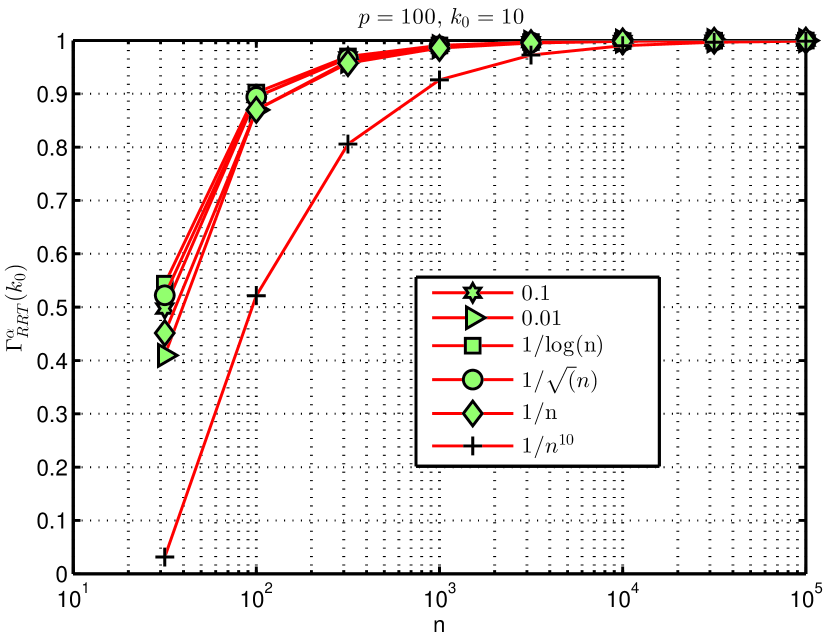
Next we discuss the behaviour of RRT as nโ†’โˆžโ†’๐‘›n\rightarrow\infty. From (6), it is clear that the extra SNR required for support recovery using RRT decreases with increasing ฮ“Rโ€‹Rโ€‹Tฮฑโ€‹(k0)superscriptsubscriptฮ“๐‘…๐‘…๐‘‡๐›ผsubscript๐‘˜0\Gamma_{RRT}^{\alpha}(k_{0}). However, by Lemma 2 increasing ฮ“Rโ€‹Rโ€‹Tฮฑโ€‹(k0)superscriptsubscriptฮ“๐‘…๐‘…๐‘‡๐›ผsubscript๐‘˜0\Gamma_{RRT}^{\alpha}(k_{0}) requires an increase in the value of ฮฑ๐›ผ\alpha. However, increasing ฮฑ๐›ผ\alpha decreases the probability of support recovery given by 1โˆ’ฮฑโˆ’1/n1๐›ผ1๐‘›1-\alpha-1/n. In other words, one cannot have exact support recovery using RRT at lower SNR without increasing the probability of error in the process. An answer to this conundrum is available in the large sample regime where it is possible to achieve both ฮฑโ‰ˆ0๐›ผ0\alpha\approx 0 and ฮ“Rโ€‹Rโ€‹Tฮฑโ€‹(k0)โ‰ˆ1superscriptsubscriptฮ“๐‘…๐‘…๐‘‡๐›ผsubscript๐‘˜01\Gamma_{RRT}^{\alpha}(k_{0})\approx 1, i.e., no extra SNR requirement and no decrease in probability of support recovery. The following theorem states the conditions required for ฮ“Rโ€‹Rโ€‹Tฮฑโ€‹(k0)โ‰ˆ1superscriptsubscriptฮ“๐‘…๐‘…๐‘‡๐›ผsubscript๐‘˜01\Gamma_{RRT}^{\alpha}(k_{0})\approx 1 for large values of n๐‘›n.

Theorem 4.

Define klโ€‹iโ€‹m=limnโ†’โˆžโ€‹k0/nsubscript๐‘˜๐‘™๐‘–๐‘šโ†’๐‘›subscript๐‘˜0๐‘›k_{lim}=\underset{n\rightarrow\infty}{\lim}k_{0}/n, plโ€‹iโ€‹m=limnโ†’โˆžโ€‹logโก(p)/nsubscript๐‘๐‘™๐‘–๐‘šโ†’๐‘›๐‘๐‘›p_{lim}=\underset{n\rightarrow\infty}{\lim}\log(p)/n and ฮฑlโ€‹iโ€‹m=limnโ†’โˆžโ€‹logโก(ฮฑ)/nsubscript๐›ผ๐‘™๐‘–๐‘šโ†’๐‘›๐›ผ๐‘›\alpha_{lim}=\underset{n\rightarrow\infty}{\lim}\log(\alpha)/n. Let kmโ€‹aโ€‹x=minโก(p,[0.5โ€‹(n+1)])subscript๐‘˜๐‘š๐‘Ž๐‘ฅ๐‘delimited-[]0.5๐‘›1k_{max}=\min(p,[0.5(n+1)]). Then ฮ“Rโ€‹Rโ€‹Tฮฑโ€‹(k0)=Fnโˆ’k02,0.5โˆ’1โ€‹(ฮฑkmโ€‹aโ€‹xโ€‹(pโˆ’k0+1))subscriptsuperscriptฮ“๐›ผ๐‘…๐‘…๐‘‡subscript๐‘˜0superscriptsubscript๐น๐‘›subscript๐‘˜020.51๐›ผsubscript๐‘˜๐‘š๐‘Ž๐‘ฅ๐‘subscript๐‘˜01\Gamma^{\alpha}_{RRT}(k_{0})=\sqrt{F_{\frac{n-k_{0}}{2},0.5}^{-1}\left(\dfrac{\alpha}{k_{max}(p-k_{0}+1)}\right)} satisfies the following asymptotic limits.
Case 1:-). limnโ†’โˆžโ€‹ฮ“Rโ€‹Rโ€‹Tฮฑโ€‹(k0)=1โ†’๐‘›subscriptsuperscriptฮ“๐›ผ๐‘…๐‘…๐‘‡subscript๐‘˜01\underset{n\rightarrow\infty}{\lim}\Gamma^{\alpha}_{RRT}(k_{0})=1, whenever klโ€‹iโ€‹m<0.5subscript๐‘˜๐‘™๐‘–๐‘š0.5k_{lim}<0.5, plโ€‹iโ€‹m=0subscript๐‘๐‘™๐‘–๐‘š0p_{lim}=0 and ฮฑlโ€‹iโ€‹m=0subscript๐›ผ๐‘™๐‘–๐‘š0\alpha_{lim}=0.
Case 2:-). 0<limnโ†’โˆžโ€‹ฮ“Rโ€‹Rโ€‹Tฮฑโ€‹(k0)<10โ†’๐‘›subscriptsuperscriptฮ“๐›ผ๐‘…๐‘…๐‘‡subscript๐‘˜010<\underset{n\rightarrow\infty}{\lim}\Gamma^{\alpha}_{RRT}(k_{0})<1 if klโ€‹iโ€‹m<0.5subscript๐‘˜๐‘™๐‘–๐‘š0.5k_{lim}<0.5, ฮฑlโ€‹iโ€‹m=0subscript๐›ผ๐‘™๐‘–๐‘š0\alpha_{lim}=0 and plโ€‹iโ€‹m>0subscript๐‘๐‘™๐‘–๐‘š0p_{lim}>0. In particular, limnโ†’โˆžโ€‹ฮ“Rโ€‹Rโ€‹Tฮฑโ€‹(k0)=expโก(โˆ’plโ€‹iโ€‹m1โˆ’klโ€‹iโ€‹m)โ†’๐‘›superscriptsubscriptฮ“๐‘…๐‘…๐‘‡๐›ผsubscript๐‘˜0subscript๐‘๐‘™๐‘–๐‘š1subscript๐‘˜๐‘™๐‘–๐‘š\underset{n\rightarrow\infty}{\lim}\Gamma_{RRT}^{\alpha}(k_{0})=\exp(\frac{-p_{lim}}{1-k_{lim}}).
Case 3:- limnโ†’โˆžโ€‹ฮ“Rโ€‹Rโ€‹Tฮฑโ€‹(k0)=0โ†’๐‘›subscriptsuperscriptฮ“๐›ผ๐‘…๐‘…๐‘‡subscript๐‘˜00\underset{n\rightarrow\infty}{\lim}\Gamma^{\alpha}_{RRT}(k_{0})=0 if klโ€‹iโ€‹m<0.5subscript๐‘˜๐‘™๐‘–๐‘š0.5k_{lim}<0.5, ฮฑlโ€‹iโ€‹m=0subscript๐›ผ๐‘™๐‘–๐‘š0\alpha_{lim}=0 and plโ€‹iโ€‹m=โˆžsubscript๐‘๐‘™๐‘–๐‘šp_{lim}=\infty.

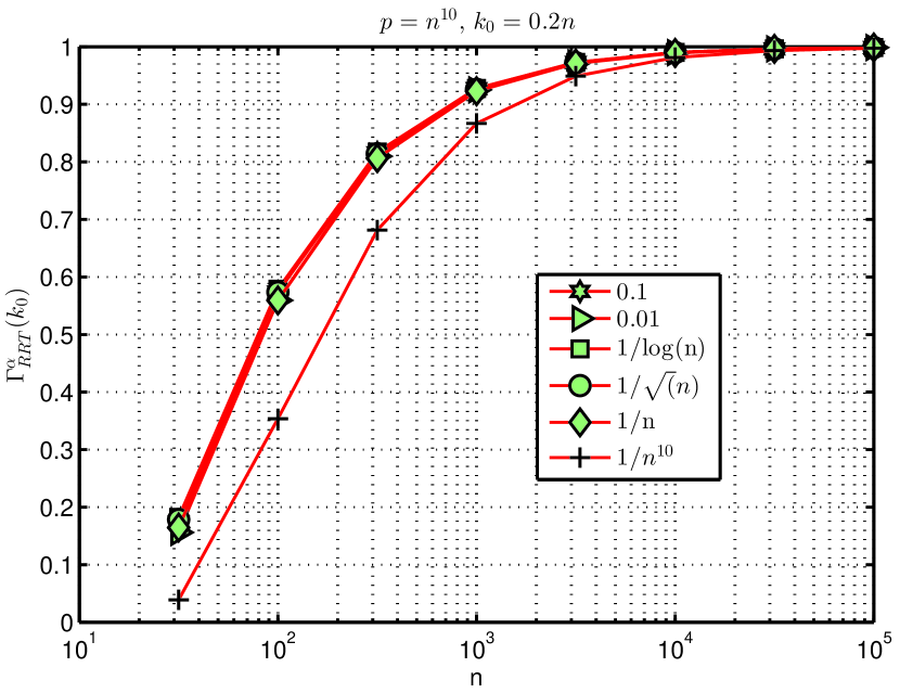
Theorem 4 states that all choices of (n,p,k0)๐‘›๐‘subscript๐‘˜0(n,p,k_{0}) satisfying plโ€‹iโ€‹m=0subscript๐‘๐‘™๐‘–๐‘š0p_{lim}=0 and klโ€‹iโ€‹m<0.5subscript๐‘˜๐‘™๐‘–๐‘š0.5k_{lim}<0.5 can result in limnโ†’โˆžโ€‹ฮ“Rโ€‹Rโ€‹Tฮฑโ€‹(k0)=1โ†’๐‘›subscriptsuperscriptฮ“๐›ผ๐‘…๐‘…๐‘‡subscript๐‘˜01\underset{n\rightarrow\infty}{\lim}\Gamma^{\alpha}_{RRT}(k_{0})=1 provided that the parameter ฮฑ๐›ผ\alpha satisfies ฮฑlโ€‹iโ€‹m=0subscript๐›ผ๐‘™๐‘–๐‘š0\alpha_{lim}=0. Note that ฮฑlโ€‹iโ€‹m=0subscript๐›ผ๐‘™๐‘–๐‘š0\alpha_{lim}=0 for a wide variety of ฮฑ๐›ผ\alpha including ฮฑ=constant๐›ผconstant\alpha=\text{constant}, ฮฑ=1/nฮด๐›ผ1superscript๐‘›๐›ฟ\alpha=1/n^{\delta} for some ฮด>0๐›ฟ0\delta>0, ฮฑ=1/logโก(n)๐›ผ1๐‘›\alpha=1/\log(n) etc. It is interesting to see which (n,p,k0)๐‘›๐‘subscript๐‘˜0(n,p,k_{0}) scenario gives plโ€‹iโ€‹m=0subscript๐‘๐‘™๐‘–๐‘š0p_{lim}=0 and klโ€‹iโ€‹m<0.5subscript๐‘˜๐‘™๐‘–๐‘š0.5k_{lim}<0.5. Note that exact recovery in n<p๐‘›๐‘n<p scenario is possible only if k0โ‰ค[0.5โ€‹(n+1)]subscript๐‘˜0delimited-[]0.5๐‘›1k_{0}\leq[0.5(n+1)]. Thus, the assumption klโ€‹iโ€‹m<0.5subscript๐‘˜๐‘™๐‘–๐‘š0.5k_{lim}<0.5 will be satisfied in all interesting problem scenarios.

Regime 1:- limnโ†’โˆžโ€‹ฮ“Rโ€‹Rโ€‹Tฮฑโ€‹(k0)=1โ†’๐‘›superscriptsubscriptฮ“๐‘…๐‘…๐‘‡๐›ผsubscript๐‘˜01\underset{n\rightarrow\infty}{\lim}\Gamma_{RRT}^{\alpha}(k_{0})=1 in low dimensional regression problems with p๐‘p fixed and nโ†’โˆžโ†’๐‘›n\rightarrow\infty or all (n,p)โ†’(โˆž,โˆž)โ†’๐‘›๐‘(n,p)\rightarrow(\infty,\infty) with limnโ†’โˆžโ€‹p/nโ‰ค1โ†’๐‘›๐‘๐‘›1\underset{n\rightarrow\infty}{\lim}p/n\leq 1.
Regime 2:- limnโ†’โˆžโ€‹ฮ“Rโ€‹Rโ€‹Tฮฑโ€‹(k0)=1โ†’๐‘›superscriptsubscriptฮ“๐‘…๐‘…๐‘‡๐›ผsubscript๐‘˜01\underset{n\rightarrow\infty}{\lim}\Gamma_{RRT}^{\alpha}(k_{0})=1 in high dimensional case with p๐‘p increases sub exponentially with n๐‘›n as expโก(nฮด)superscript๐‘›๐›ฟ\exp(n^{\delta}) for some ฮด<1๐›ฟ1\delta<1 or p๐‘p increases polynomially w.r.t n๐‘›n, i.e., p=nฮด๐‘superscript๐‘›๐›ฟp=n^{\delta} for some ฮด>1๐›ฟ1\delta>1. In both cases, plโ€‹iโ€‹m=limnโ†’โˆžโ€‹logโก(nฮด)/n=0subscript๐‘๐‘™๐‘–๐‘šโ†’๐‘›superscript๐‘›๐›ฟ๐‘›0p_{lim}=\underset{n\rightarrow\infty}{\lim}\log(n^{\delta})/n=0 and plโ€‹iโ€‹m=limnโ†’โˆžโ€‹logโก(expโก(nฮด))/n=0subscript๐‘๐‘™๐‘–๐‘šโ†’๐‘›superscript๐‘›๐›ฟ๐‘›0p_{lim}=\underset{n\rightarrow\infty}{\lim}\log(\exp(n^{\delta}))/n=0.
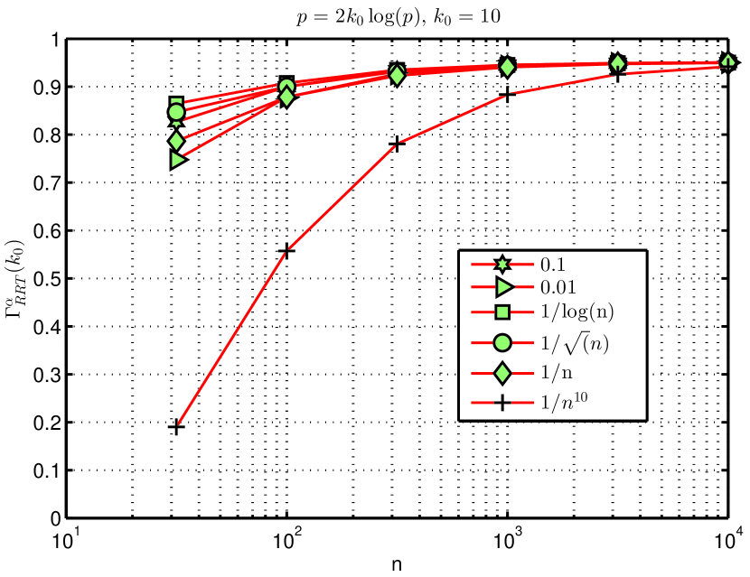
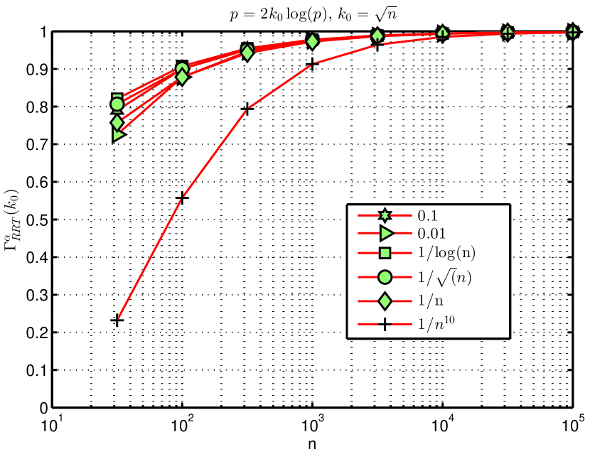
Regime 3:- limnโ†’โˆžโ€‹ฮ“Rโ€‹Rโ€‹Tฮฑโ€‹(k0)=1โ†’๐‘›superscriptsubscriptฮ“๐‘…๐‘…๐‘‡๐›ผsubscript๐‘˜01\underset{n\rightarrow\infty}{\lim}\Gamma_{RRT}^{\alpha}(k_{0})=1 in the extreme high dimensional case where (n,p,k0)โ†’(โˆž,โˆž,โˆž)โ†’๐‘›๐‘subscript๐‘˜0(n,p,k_{0})\rightarrow(\infty,\infty,\infty) satisfying nโ‰ฅcโ€‹k0โ€‹logโก(p)๐‘›๐‘subscript๐‘˜0๐‘n\geq ck_{0}\log(p) for some constant c>0๐‘0c>0. Here plโ€‹iโ€‹m=limnโ†’โˆžโ€‹logโก(p)/nโ‰คlimnโ†’โˆžโ€‹1cโ€‹k0=0subscript๐‘๐‘™๐‘–๐‘šโ†’๐‘›๐‘๐‘›โ†’๐‘›1๐‘subscript๐‘˜00p_{lim}=\underset{n\rightarrow\infty}{\lim}\log(p)/n\leq\underset{n\rightarrow\infty}{\lim}\dfrac{1}{ck_{0}}=0 and klโ€‹iโ€‹m=limnโ†’โˆžโ€‹1/cโ€‹logโก(p)=0subscript๐‘˜๐‘™๐‘–๐‘šโ†’๐‘›1๐‘๐‘0k_{lim}=\underset{n\rightarrow\infty}{\lim}1/c\log(p)=0. Note that the sampling regime nโ‰ˆ2โ€‹k0โ€‹logโก(p)๐‘›2subscript๐‘˜0๐‘n\approx 2k_{0}\log(p) is the best known asymptotic guarantee available for OMP(Fletcher & Rangan, 2012).
Regime 4:- Consider a sampling regime where (n,p)โ†’(โˆž,โˆž)โ†’๐‘›๐‘(n,p)\rightarrow(\infty,\infty) such that k0subscript๐‘˜0k_{0} is fixed and n=cโ€‹k0โ€‹logโก(p)๐‘›๐‘subscript๐‘˜0๐‘n=ck_{0}\log(p), i.e., p๐‘p is exponentially increasing with n๐‘›n. Here plโ€‹iโ€‹m=1/(cโ€‹k0)subscript๐‘๐‘™๐‘–๐‘š1๐‘subscript๐‘˜0p_{lim}=1/(ck_{0}) and klim=0subscript๐‘˜0k_{\lim}=0. Consequently, limnโ†’โˆžโ€‹ฮ“Rโ€‹Rโ€‹Tฮฑโ€‹(k0)=expโก(โˆ’1cโ€‹k0)<1โ†’๐‘›superscriptsubscriptฮ“๐‘…๐‘…๐‘‡๐›ผsubscript๐‘˜01๐‘subscript๐‘˜01\underset{n\rightarrow\infty}{\lim}\Gamma_{RRT}^{\alpha}(k_{0})=\exp\left(\frac{-1}{ck_{0}}\right)<1. A good example of this sampling regime is (Tropp & Gilbert, 2007) where it was shown that OMP can recover a (not every) particular k0subscript๐‘˜0k_{0} dimensional signal from n๐‘›n random measurements (in noiseless case) when n=cโ€‹k0โ€‹logโก(p)๐‘›๐‘subscript๐‘˜0๐‘n=ck_{0}\log(p). Note that cโ‰ค20๐‘20c\leq 20 for all k0subscript๐‘˜0k_{0} and cโ‰ˆ4๐‘4c\approx 4 for large k0subscript๐‘˜0k_{0}. Even if we assume that only n=4โ€‹k0โ€‹logโก(p)๐‘›4subscript๐‘˜0๐‘n=4k_{0}\log(p) measurements are sufficient for recovering a k0subscript๐‘˜0k_{0} sparse signal, we have limnโ†’โˆžโ€‹ฮ“Rโ€‹Rโ€‹Tฮฑโ€‹(k0)=expโก(โˆ’0.125)=0.9512โ†’๐‘›superscriptsubscriptฮ“๐‘…๐‘…๐‘‡๐›ผsubscript๐‘˜00.1250.9512\underset{n\rightarrow\infty}{\lim}\Gamma_{RRT}^{\alpha}(k_{0})=\exp(-0.125)=0.9512 for k0=5subscript๐‘˜05k_{0}=5 (i.e., ฯตeโ€‹xโ€‹tโ€‹rโ€‹aโ‰ค1.0257subscriptitalic-ฯต๐‘’๐‘ฅ๐‘ก๐‘Ÿ๐‘Ž1.0257\epsilon_{extra}\leq 1.0257) and limnโ†’โˆžโ€‹ฮ“Rโ€‹Rโ€‹Tฮฑโ€‹(k0)=expโก(โˆ’0.125)=0.9753โ†’๐‘›superscriptsubscriptฮ“๐‘…๐‘…๐‘‡๐›ผsubscript๐‘˜00.1250.9753\underset{n\rightarrow\infty}{\lim}\Gamma_{RRT}^{\alpha}(k_{0})=\exp(-0.125)=0.9753 for k0=10subscript๐‘˜010k_{0}=10 (i.e.,ฯตeโ€‹xโ€‹tโ€‹rโ€‹aโ‰ค1.0127subscriptitalic-ฯต๐‘’๐‘ฅ๐‘ก๐‘Ÿ๐‘Ž1.0127\epsilon_{extra}\leq 1.0127).

Note that ฮ“Rโ€‹Rโ€‹Tฮฑโ€‹(k0)โ†’1โ†’superscriptsubscriptฮ“๐‘…๐‘…๐‘‡๐›ผsubscript๐‘˜01\Gamma_{RRT}^{\alpha}(k_{0})\rightarrow 1 as nโ†’โˆžโ†’๐‘›n\rightarrow\infty implies that ฯตeโ€‹xโ€‹tโ€‹rโ€‹aโ†’1โ†’subscriptitalic-ฯต๐‘’๐‘ฅ๐‘ก๐‘Ÿ๐‘Ž1\epsilon_{extra}\rightarrow 1 and minโก(ฯตoโ€‹mโ€‹p,ฯตrโ€‹rโ€‹t)โ†’1โ†’subscriptitalic-ฯต๐‘œ๐‘š๐‘subscriptitalic-ฯต๐‘Ÿ๐‘Ÿ๐‘ก1\min(\epsilon_{omp},\epsilon_{rrt})\rightarrow 1. This asymptotic behaviour of ฮ“Rโ€‹Rโ€‹Tฮฑโ€‹(k0)superscriptsubscriptฮ“๐‘…๐‘…๐‘‡๐›ผsubscript๐‘˜0\Gamma_{RRT}^{\alpha}(k_{0}) and ฯตeโ€‹xโ€‹tโ€‹rโ€‹asubscriptitalic-ฯต๐‘’๐‘ฅ๐‘ก๐‘Ÿ๐‘Ž\epsilon_{extra} imply the large sample consistency of RRT as stated in the following theorem.

Theorem 5.

Suppose that the sample size nโ†’โˆžโ†’๐‘›n\rightarrow\infty such that the matrix ๐—๐—{\bf X} satisfies ฮดk0+1<1k0+1subscript๐›ฟsubscript๐‘˜011subscript๐‘˜01\delta_{k_{0}+1}<\frac{1}{\sqrt{k_{0}+1}}, ฯตฯƒโ‰คฯตoโ€‹mโ€‹psubscriptitalic-ฯต๐œŽsubscriptitalic-ฯต๐‘œ๐‘š๐‘\epsilon_{\sigma}\leq\epsilon_{omp} and plโ€‹iโ€‹m=0subscript๐‘๐‘™๐‘–๐‘š0p_{lim}=0. Then,
a). OMP running k0subscript๐‘˜0k_{0} iterations and OMP with SC โ€–๐ซkโ€–2โ‰คฯตฯƒsubscriptnormsuperscript๐ซ๐‘˜2subscriptitalic-ฯต๐œŽ\|{\bf r}^{k}\|_{2}\leq\epsilon_{\sigma} are large sample consistent, i.e.. limnโ†’โˆžโ€‹โ„™โ€‹(๐’ฎ^=๐’ฎ)=1โ†’๐‘›โ„™^๐’ฎ๐’ฎ1\underset{n\rightarrow\infty}{\lim}\mathbb{P}(\hat{\mathcal{S}}=\mathcal{S})=1.
b). RRT with hyper parameter ฮฑ๐›ผ\alpha satisfying limnโ†’โˆžโ€‹ฮฑ=0โ†’๐‘›๐›ผ0\underset{n\rightarrow\infty}{\lim}\alpha=0 and ฮฑlโ€‹iโ€‹m=0subscript๐›ผ๐‘™๐‘–๐‘š0\alpha_{lim}=0 is also large sample consistent.

Theorem 5 implies that at large sample sizes, RRT can accomplish exact support recovery under the same SNR and matrix conditions required by OMP with a priori knowledge of k0subscript๐‘˜0k_{0} or ฯƒ2superscript๐œŽ2\sigma^{2}. Theorem 5 has a very important corollary.

Remark 5.

Theorem 1 implies that all choices of ฮฑ๐›ผ\alpha satisfying ฮฑโ†’0โ†’๐›ผ0\alpha\rightarrow 0 and ฮฑlโ€‹iโ€‹m=0subscript๐›ผ๐‘™๐‘–๐‘š0\alpha_{lim}=0 deliver similar performances as nโ†’โˆžโ†’๐‘›n\rightarrow\infty. Note that the range of adaptations satisfying ฮฑโ†’0โ†’๐›ผ0\alpha\rightarrow 0 and ฮฑlโ€‹iโ€‹m=0subscript๐›ผ๐‘™๐‘–๐‘š0\alpha_{lim}=0 include ฮฑ=1/logโก(n)๐›ผ1๐‘›\alpha=1/\log(n), ฮฑ=1/nฮด๐›ผ1superscript๐‘›๐›ฟ\alpha=1/n^{\delta} for ฮด>0๐›ฟ0\delta>0 etc. Since a very wide range of tuning parameters deliver similar results as nโ†’โˆžโ†’๐‘›n\rightarrow\infty, RRT is in fact asymptotically tuning free.

Remark 6.

Based on the large sample analysis of RRT, one can make the following guidelines on the choice of ฮฑ๐›ผ\alpha. When the sample size n๐‘›n is large, one can choose ฮฑ๐›ผ\alpha as a function of n๐‘›n that satisfies both limnโ†’โˆžโ€‹ฮฑ=0โ†’๐‘›๐›ผ0\underset{n\rightarrow\infty}{\lim}\alpha=0 and ฮฑlโ€‹iโ€‹m=0subscript๐›ผ๐‘™๐‘–๐‘š0\alpha_{lim}=0. Also since the support recovery guarantees are of the form 1โˆ’1/nโˆ’ฮฑ11๐‘›๐›ผ1-1/n-\alpha, it does not make sense to choose a value of ฮฑ๐›ผ\alpha that decays to zero faster than 1/n1๐‘›1/n. Hence, it is preferable to choose values of ฮฑ๐›ผ\alpha that decreases to zero slower than 1/n1๐‘›1/n like ฮฑ=1/logโก(n)๐›ผ1๐‘›\alpha=1/\log(n), ฮฑ=1/n๐›ผ1๐‘›\alpha=1/\sqrt{n} etc.

4.2 A high SNR operational interpretation of ฮฑ๐›ผ\alpha

Having discussed the large sample behaviour of RRT, we next discuss the finite sample and high SNR behaviour of RRT. Define the events support recovery error โ„ฐ={๐’ฎ^โ‰ ๐’ฎ}โ„ฐ^๐’ฎ๐’ฎ\mathcal{E}=\{\hat{\mathcal{S}}\neq\mathcal{S}\} and false positive โ„ฑ=cโ€‹aโ€‹rโ€‹dโ€‹(๐’ฎ^/๐’ฎ)>0โ„ฑ๐‘๐‘Ž๐‘Ÿ๐‘‘^๐’ฎ๐’ฎ0\mathcal{F}=card(\hat{\mathcal{S}}/\mathcal{S})>0 and missed discovery or false negative โ„ณ=cโ€‹aโ€‹rโ€‹dโ€‹(๐’ฎ/๐’ฎ^)>0โ„ณ๐‘๐‘Ž๐‘Ÿ๐‘‘๐’ฎ^๐’ฎ0\mathcal{M}=card(\mathcal{S}/\hat{\mathcal{S}})>0. The following theorem characterizes the likelihood of these events as SNR increases to infinity or ฯƒ2โ†’0โ†’superscript๐œŽ20\sigma^{2}\rightarrow 0.

Theorem 6.

Let kmโ€‹aโ€‹x>k0subscript๐‘˜๐‘š๐‘Ž๐‘ฅsubscript๐‘˜0k_{max}>k_{0} and the matrix ๐—๐—{\bf X} satisfies ฮดk0+1<1/k0+1subscript๐›ฟsubscript๐‘˜011subscript๐‘˜01\delta_{k_{0}+1}<{1}/{\sqrt{k_{0}+1}}. Then,
a). limฯƒ2โ†’0โ€‹โ„™โ€‹(โ„ณ)=0โ†’superscript๐œŽ20โ„™โ„ณ0\underset{\sigma^{2}\rightarrow 0}{\lim}\mathbb{P}(\mathcal{M})=0.
b). limฯƒ2โ†’0โ€‹โ„™โ€‹(โ„ฐ)=limฯƒ2โ†’0โ€‹โ„™โ€‹(โ„ฑ)โ‰คฮฑโ†’superscript๐œŽ20โ„™โ„ฐโ†’superscript๐œŽ20โ„™โ„ฑ๐›ผ\underset{\sigma^{2}\rightarrow 0}{\lim}\mathbb{P}(\mathcal{E})=\underset{\sigma^{2}\rightarrow 0}{\lim}\mathbb{P}(\mathcal{F})\leq\alpha.

Theorem 6 states that when the matrix ๐—๐—{\bf X} allows for exact support recovery in the noiseless or low noise situation, RRT will not suffer from missed discoveries. Under such favourable conditions, ฮฑ๐›ผ\alpha is a high SNR upper bound on both the probability of error and the probability of false positives. Please note that such explicit characterization of hyper parameters are not available for hyper parameters in Square root LASSO, RAT, LAT etc.
Refer to caption
Refer to caption
Refer to caption
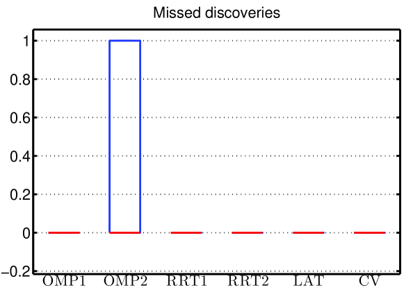
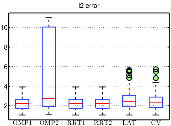
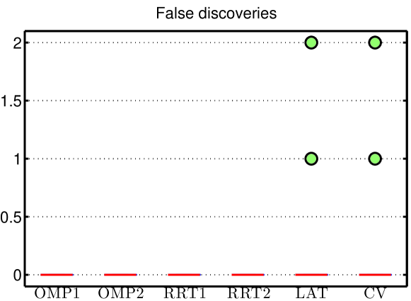
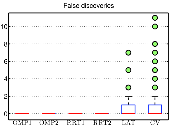
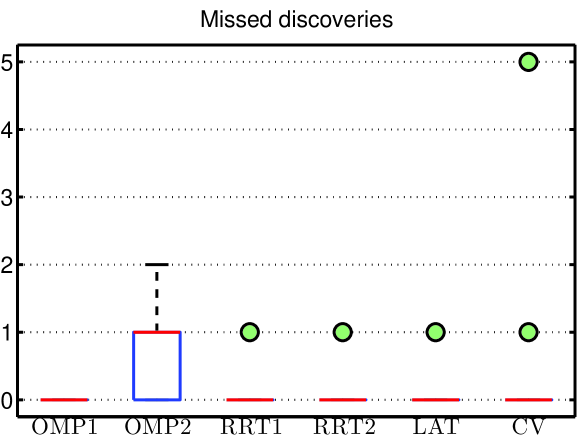
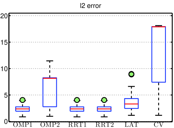
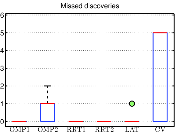
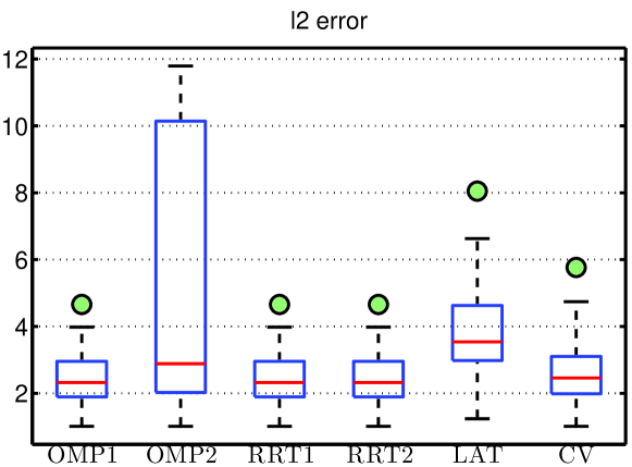
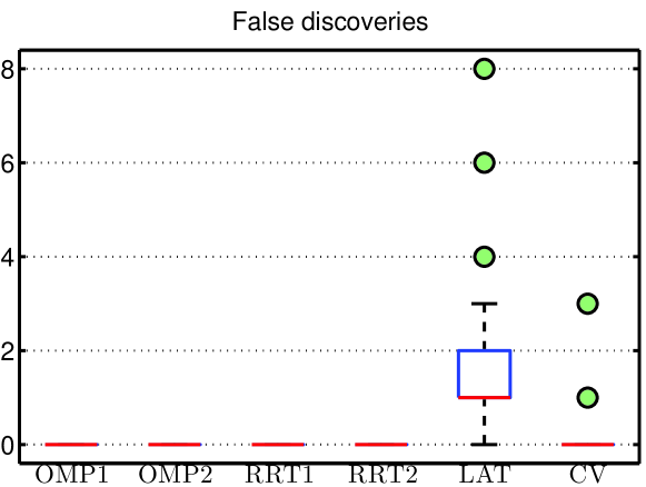
Figure 1: Experiment 1: Box plots of l2subscript๐‘™2l_{2} error โ€–๐œท^โˆ’๐œทโ€–2subscriptnorm^๐œท๐œท2\|\hat{\bm{\beta}}-\bm{\beta}\|_{2} (left), false positives (middle) and false negatives (right) .
Refer to caption
Refer to caption
Refer to caption
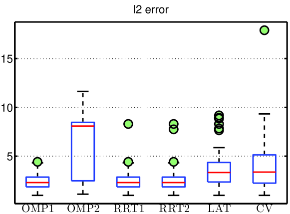
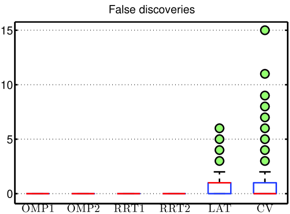
Figure 2: Experiment 2: Box plots of l2subscript๐‘™2l_{2} error โ€–๐œท^โˆ’๐œทโ€–2subscriptnorm^๐œท๐œท2\|\hat{\bm{\beta}}-\bm{\beta}\|_{2} (left), false positives (middle) and false negatives (right) .
Refer to caption
Refer to caption
Refer to caption
Figure 3: Experiment 3: Box plots of l2subscript๐‘™2l_{2} error โ€–๐œท^โˆ’๐œทโ€–2subscriptnorm^๐œท๐œท2\|\hat{\bm{\beta}}-\bm{\beta}\|_{2} (left), false positives (middle) and false negatives (right) .
Refer to caption
Refer to caption
Refer to caption
Figure 4: Experiment 4: Box plots of l2subscript๐‘™2l_{2} error โ€–๐œท^โˆ’๐œทโ€–2subscriptnorm^๐œท๐œท2\|\hat{\bm{\beta}}-\bm{\beta}\|_{2} (left), false positives (middle) and false negatives (right) .
Data Set Outliers reported in literature RRT CV LAT
Stack Loss 1, 3, 4, 21 1, 3, 4, 21 1, 3, 4, 21 4, 21
n=21๐‘›21n=21 and p=4๐‘4p=4 (Rousseeuw & Leroy, 2005) plus 10 observations
including intercept
(Rousseeuw & Leroy, 2005)
AR2000 9, 21, 30, 31, 38, 47 9, 14, 21, 30 9, 21, 30, 31, 38, 47 9, 14, 21
n=60๐‘›60n=60 and p=3๐‘3p=3 31, 38, 47, 50 plus 41 observations 30, 31, 38
(Atkinson & Riani, 2012) (Atkinson & Riani, 2012) 47, 50
Brain Body Weight 1, 6, 14, 16, 17, 25 1, 6, 16, 25 1, 6, 16, 25 1, 6, 16, 25
n=27๐‘›27n=27 and p=1๐‘1p=1
(Rousseeuw & Leroy, 2005) (Rousseeuw & Leroy, 2005)
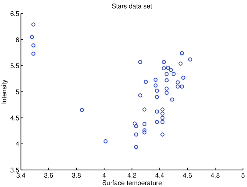
Stars 11, 20, 30, 34 11, 20, 30, 34 11, 20, 30, 34 11, 20, 30, 34
n0=47subscript๐‘›047n_{0}=47 and p0=1subscript๐‘01p_{0}=1 plus 31 observations
(Rousseeuw & Leroy, 2005) (Rousseeuw & Leroy, 2005)
Table 1: Outliers detected by various algorithms. RRT with both ฮฑ=1/logโก(n)๐›ผ1๐‘›\alpha=1/\log(n) and ฮฑ=1/n๐›ผ1๐‘›\alpha=1/\sqrt{n} delivered similar results. Existing results on Stack loss, Brain and Body weight and Stars data set are based on the combinatorially complex least median of squares (LMedS) algorithm. Existing results on AR2000 are based on extensive graphical analysis.

5 Numerical simulations

In this section, we provide extensive numerical simulations comparing the performance of RRT with state of art sparse recovery techniques. In particular, we compare the performance of RRT with OMP with k0subscript๐‘˜0k_{0} estimated using five fold CV and the least squares adaptive thresholding (LAT) proposed in (Wang etย al., 2016). In synthetic data sets, we also compare RRT with OMP running exactly k0subscript๐‘˜0k_{0} iterations and OMP with SC โ€–๐ซkโ€–2โ‰คฯƒโ€‹n+2โ€‹nโ€‹logโก(n)subscriptnormsuperscript๐ซ๐‘˜2๐œŽ๐‘›2๐‘›๐‘›\|{\bf r}^{k}\|_{2}\leq\sigma\sqrt{n+2\sqrt{n\log(n)}}(Cai & Wang, 2011). These algorithms are denoted in Figures 1-4 by โ€œCVโ€, โ€œLATโ€, โ€œOMP1โ€ and โ€œOMP2โ€ respectively. RRT1 and RRT2 represent RRT with parameter ฮฑ๐›ผ\alpha set to ฮฑ=1/logโก(n)๐›ผ1๐‘›\alpha=1/\log(n) and ฮฑ=1/n๐›ผ1๐‘›\alpha=1/\sqrt{n} respectively. By Theorem 5, RRT1 and RRT2 are large sample consistent.

5.1 Synthetic data sets

The synthetic data sets are generated as follows. We consider two models for the matrix ๐—๐—{\bf X}. Model 1 sample each entry of the design matrix ๐—โˆˆโ„nร—p๐—superscriptโ„๐‘›๐‘{\bf X}\in\mathbb{R}^{n\times p} independently according to ๐’ฉโ€‹(0,1)๐’ฉ01\mathcal{N}(0,1). Matrix ๐—๐—{\bf X} in Model 2 is formed by concatenating ๐ˆnsubscript๐ˆ๐‘›{\bf I}_{n} with a nร—n๐‘›๐‘›n\times n Hadamard matrix ๐‡nsubscript๐‡๐‘›{\bf H}_{n}, i.e., ๐—=[๐ˆn,๐‡n]๐—subscript๐ˆ๐‘›subscript๐‡๐‘›{\bf X}=[{\bf I}_{n},{\bf H}_{n}]. This matrix guarantee exact support recovery using OMP at high SNR once k0<1+n2subscript๐‘˜01๐‘›2k_{0}<\frac{1+\sqrt{n}}{2}(Elad, 2010). The columns of ๐—๐—{\bf X} in both models are normalised to have unit l2subscript๐‘™2l_{2}-norm. Based on the choice of ๐—๐—{\bf X} and support ๐’ฎ๐’ฎ\mathcal{S}, we conduct 4 experiments. Experiments 1-2 involve matrix of model 1 with (n,p)๐‘›๐‘(n,p) given by (200,300)200300(200,300) and (200,900)200900(200,900) respectively with support ๐’ฎ๐’ฎ\mathcal{S} sampled randomly from the set {1,โ€ฆ,p}1โ€ฆ๐‘\{1,\dotsc,p\}. Experiment 3 and 4 involve matrix of model 2 with (n=128,p=256)formulae-sequence๐‘›128๐‘256(n=128,p=256). For experiment 3, support ๐’ฎ๐’ฎ\mathcal{S} is sampled randomly from the set {1,โ€ฆ,p}1โ€ฆ๐‘\{1,\dotsc,p\}, whereas, in experiment 4, support ๐’ฎ๐’ฎ\mathcal{S} is fixed at {1,2,โ€ฆ,k0}12โ€ฆsubscript๐‘˜0\{1,2,\dotsc,k_{0}\}. The noise ๐ฐ๐ฐ{\bf w} is sampled according to ๐’ฉโ€‹(๐ŸŽn,ฯƒ2โ€‹๐ˆn)๐’ฉsubscript0๐‘›superscript๐œŽ2subscript๐ˆ๐‘›\mathcal{N}({\bf 0}_{n},\sigma^{2}{\bf I}_{n}) with ฯƒ2=1superscript๐œŽ21\sigma^{2}=1. The non zero entries of ๐œท๐œท\bm{\beta} are randomly assigned ๐œทj=ยฑ1subscript๐œท๐‘—plus-or-minus1\bm{\beta}_{j}=\pm 1. Subsequently, these entries are scaled to achieve Sโ€‹Nโ€‹R=โ€–๐—โ€‹๐œทโ€–22/n=3๐‘†๐‘๐‘…superscriptsubscriptnorm๐—๐œท22๐‘›3SNR={\|{\bf X}\bm{\beta}\|_{2}^{2}}/n=3. The number of non zero entries k0subscript๐‘˜0k_{0} in all experiments are fixed at six. We compare the algorithms in terms of the l2subscript๐‘™2l_{2} error, the number of false positives and the number of false negatives produced in 100 runs of each experiment.

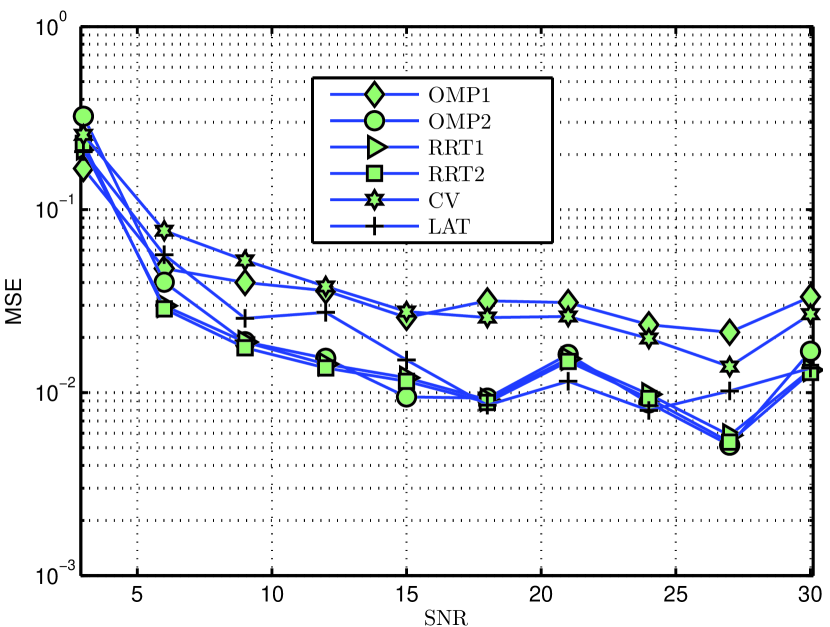
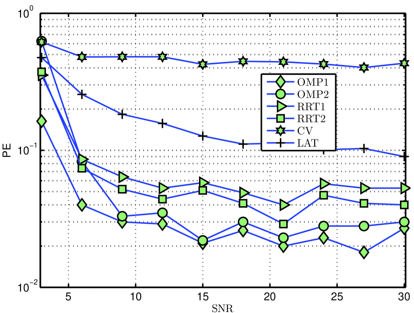
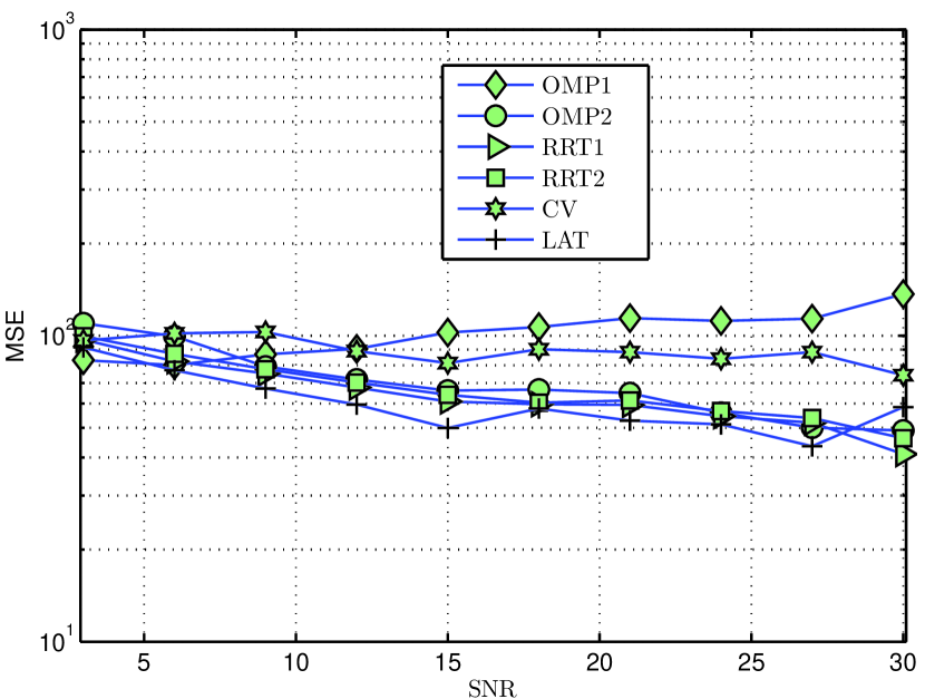
From the box plots given in Figures 1-4, it is clear that RRT with both values of ฮฑ๐›ผ\alpha perform very similar to OMP1. They differ only in one run of experiment 3 where RRT1 and RRT2 suffer from a false negative. Further, RRT1 and RRT2 outperform CV and LAT in all the four experiments in terms of all the three metrics considered for evaluation. This is primarily because LAT and CV are more prone to make false positives, whereas RRT1 and RRT2 does not report any false positives. OMP2 consistently made false negatives which explains its poor performance in terms of l2subscript๐‘™2l_{2} error. We have observed that once the SNR is made slightly higher, OMP2 delivers a performance similar to OMP1. Also note that RRT with two significantly different choices of ฮฑ๐›ผ\alpha viz. ฮฑ=1/n๐›ผ1๐‘›\alpha=1/\sqrt{n} and ฮฑ=1/logโก(n)๐›ผ1๐‘›\alpha=1/\log(n) delivered similar performances. This observation is in agreement with the claim of asymptotic tuning freeness made in Remark 5. Similar trends are also visible in the simulation results presented in supplementary materials.

5.2 Outlier detection in real data sets

We next consider the application of sparse estimation techniques including RRT to identify outliers in low dimensional or full column rank (i.e., n>p๐‘›๐‘n>p) real life data sets, an approach first considered in (Mitra etย al., 2010, 2013). Consider a robust regression model of the form ๐ฒ=๐—โ€‹๐œท+๐ฐ+๐ oโ€‹uโ€‹t๐ฒ๐—๐œท๐ฐsubscript๐ ๐‘œ๐‘ข๐‘ก{\bf y}={\bf X}\bm{\beta}+{\bf w}+{\bf g}_{out} with usual interpretations for ๐—๐—{\bf X}, ๐œท๐œท\bm{\beta} and ๐ฐ๐ฐ{\bf w}. The extra term ๐ oโ€‹uโ€‹tโˆˆโ„nsubscript๐ ๐‘œ๐‘ข๐‘กsuperscriptโ„๐‘›{\bf g}_{out}\in\mathbb{R}^{n} represents the gross errors in the regression model that cannot be modelled using the distributional assumptions on ๐ฐ๐ฐ{\bf w}. Outlier detection problem in linear regression refers to the identification of the support ๐’ฎg=sโ€‹uโ€‹pโ€‹pโ€‹(๐ oโ€‹uโ€‹t)subscript๐’ฎ๐‘”๐‘ ๐‘ข๐‘๐‘subscript๐ ๐‘œ๐‘ข๐‘ก\mathcal{S}_{g}=supp({\bf g}_{out}). Since ๐—๐—{\bf X} has full rank, one can always annihilate the signal component ๐—โ€‹๐œท๐—๐œท{\bf X}\bm{\beta} by projecting onto a subspace orthogonal to sโ€‹pโ€‹aโ€‹nโ€‹(๐—)๐‘ ๐‘๐‘Ž๐‘›๐—span({\bf X}). This will result in a simple linear regression model of the form given by

๐ฒ~=(๐ˆnโˆ’๐—๐—โ€ )โ€‹๐ฒ=(๐ˆnโˆ’๐—๐—โ€ )โ€‹๐ oโ€‹uโ€‹t+(๐ˆnโˆ’๐—๐—โ€ )โ€‹๐ฐ,~๐ฒsubscript๐ˆ๐‘›superscript๐—๐—โ€ ๐ฒsubscript๐ˆ๐‘›superscript๐—๐—โ€ subscript๐ ๐‘œ๐‘ข๐‘กsubscript๐ˆ๐‘›superscript๐—๐—โ€ ๐ฐ\tilde{\bf y}=({\bf I}_{n}-{\bf X}{\bf X}^{\dagger}){\bf y}=({\bf I}_{n}-{\bf X}{\bf X}^{\dagger}){\bf g}_{out}+({\bf I}_{n}-{\bf X}{\bf X}^{\dagger}){\bf w}, (7)

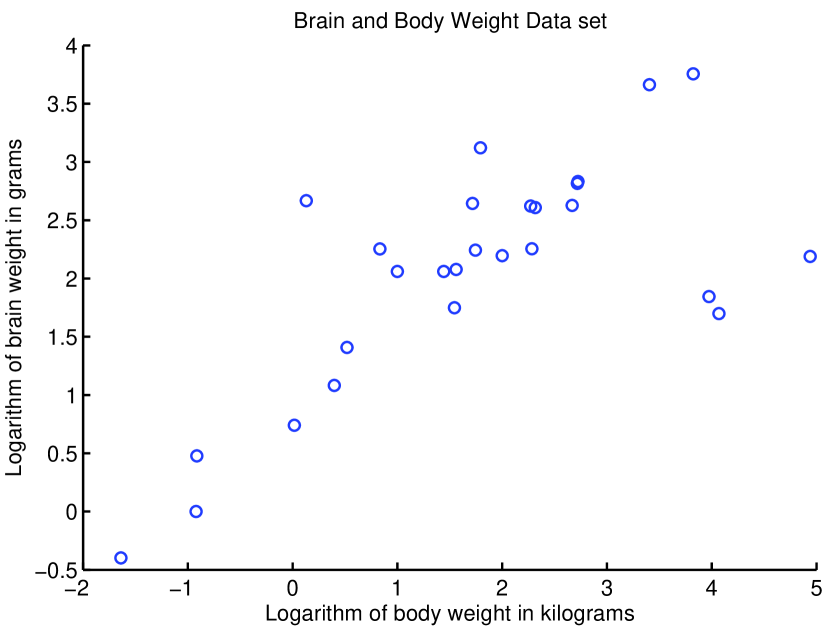
i.e., identifying ๐’ฎgsubscript๐’ฎ๐‘”\mathcal{S}_{g} in robust regression is equivalent to a sparse support identification problem in linear regression. Even though this is a regression problem with n๐‘›n observations and n๐‘›n variables, the design matrix (๐ˆnโˆ’๐—๐—โ€ )subscript๐ˆ๐‘›superscript๐—๐—โ€ ({\bf I}_{n}-{\bf X}{\bf X}^{\dagger}) in (7) is rank deficient (i.e., rโ€‹aโ€‹nโ€‹kโ€‹(๐ˆnโˆ’๐—๐—โ€ )=nโˆ’rโ€‹aโ€‹nโ€‹kโ€‹(X)<n๐‘Ÿ๐‘Ž๐‘›๐‘˜subscript๐ˆ๐‘›superscript๐—๐—โ€ ๐‘›๐‘Ÿ๐‘Ž๐‘›๐‘˜๐‘‹๐‘›rank({\bf I}_{n}-{\bf X}{\bf X}^{\dagger})=n-rank(X)<n). Hence, classical techniques based on LS are not useful for identifying ๐’ฎgsubscript๐’ฎ๐‘”\mathcal{S}_{g}. Since cโ€‹aโ€‹rโ€‹dโ€‹(๐’ฎg)๐‘๐‘Ž๐‘Ÿ๐‘‘subscript๐’ฎ๐‘”card(\mathcal{S}_{g}) and variance of ๐ฐ๐ฐ{\bf w} are unknown, we only consider the application of RRT, OMP with CV and LAT in detecting ๐’ฎgsubscript๐’ฎ๐‘”\mathcal{S}_{g}. We consider four widely studied real life data sets and compare the outliers identified by these algorithms with the existing and widely replicated studies on these data sets. More details on these data sets are given in the supplementary materials. The outliers detected by the aforementioned algorithms and outliers reported in existing literature are tabulated in TABLE 1.

Among the four data sets considered, outliers detected by RRT and existing results are in consensus in two data sets viz. Stack loss and Stars data sets. In AR2000 data set, RRT identifies all the outliers. However, RRT also include observations 141414 and 505050 as outliers. These identifications can be potential false positives. In Brain and Body Weight data set, RRT agrees with the existing results in 444 observations. However, RRT misses two observations viz. 141414 and 171717 which are claimed to be outliers by existing results. LAT agrees with RRT in all data sets except the stack loss data set where it missed outlier indices 111 and 333. CV correctly identified all the outliers identified by other algorithms in all four data sets. However, it made lot of false positives in three data sets. To summarize, among all the three algorithms considered, RRT delivered an outlier detection performance which is the most similar to the results reported in literature.

6 Conclusions

This article proposed a novel signal and noise statistics independent sparse recovery technique based on OMP called residual ratio thresholding and derived finite and large sample guarantees for the same. Numerical simulations in real and synthetic data sets demonstrates a highly competitive performance of RRT when compared to OMP with a priori knowledge of signal and noise statistics. The RRT technique developed in this article can be used to operate sparse recovery techniques that produce a monotonic sequence of support estimates in a signal and noise statistics oblivious fashion. However, the support estimate sequence generated by algorithms like LASSO, DS, SP etc. are not monotonic in nature. Hence, extending the concept of RRT to operate sparse estimation techniques that produce non monotonic support sequence in a signal and noise statistics oblivious fashion is an interesting direction of future research.

7 Supplementary Materials: Proofs of Theorems 1-6

7.1 Appendix A: Proof of Theorem 1

Statement of Theorem 1:- Assume that the matrix ๐—๐—{\bf X} satisfies the RIC constraint ฮดk0+1<1k0+1subscript๐›ฟsubscript๐‘˜011subscript๐‘˜01\delta_{k_{0}+1}<\dfrac{1}{\sqrt{k_{0}+1}} and kmโ€‹aโ€‹x>k0subscript๐‘˜๐‘š๐‘Ž๐‘ฅsubscript๐‘˜0k_{max}>k_{0}. Then
a). Rโ€‹Rโ€‹(kmโ€‹iโ€‹n)โ€‹โ†’๐‘ƒโ€‹0๐‘…๐‘…subscript๐‘˜๐‘š๐‘–๐‘›๐‘ƒโ†’0RR(k_{min})\overset{P}{\rightarrow}0 as ฯƒ2โ†’0โ†’superscript๐œŽ20\sigma^{2}\rightarrow 0.
b). limฯƒ2โ†’0โ€‹โ„™โ€‹(kmโ€‹iโ€‹n=k0)=1โ†’superscript๐œŽ20โ„™subscript๐‘˜๐‘š๐‘–๐‘›subscript๐‘˜01\underset{\sigma^{2}\rightarrow 0}{\lim}\mathbb{P}(k_{min}=k_{0})=1.

Proof.

We first prove statement b) of Theorem 1. By Lemma 1, we have kmโ€‹iโ€‹n=k0subscript๐‘˜๐‘š๐‘–๐‘›subscript๐‘˜0k_{min}=k_{0} once โ€–๐ฐโ€–2โ‰คฯตoโ€‹mโ€‹psubscriptnorm๐ฐ2subscriptitalic-ฯต๐‘œ๐‘š๐‘\|{\bf w}\|_{2}\leq\epsilon_{omp}. Hence, โ„™โ€‹(kmโ€‹iโ€‹n=k0)โ‰ฅโ„™โ€‹(โ€–๐ฐโ€–2โ‰คฯตoโ€‹mโ€‹p)โ„™subscript๐‘˜๐‘š๐‘–๐‘›subscript๐‘˜0โ„™subscriptnorm๐ฐ2subscriptitalic-ฯต๐‘œ๐‘š๐‘\mathbb{P}(k_{min}=k_{0})\geq\mathbb{P}(\|{\bf w}\|_{2}\leq\epsilon_{omp}). Since โ€–๐ฐโ€–2โ€‹โ†’๐‘ƒโ€‹0subscriptnorm๐ฐ2๐‘ƒโ†’0\|{\bf w}\|_{2}\overset{P}{\rightarrow}0 as ฯƒ2โ†’0โ†’superscript๐œŽ20\sigma^{2}\rightarrow 0, it follows from the definition of convergence in probability that limฯƒ2โ†’0โ€‹โ„™โ€‹(โ€–๐ฐโ€–2โ‰คฯตoโ€‹mโ€‹p)=1โ†’superscript๐œŽ20โ„™subscriptnorm๐ฐ2subscriptitalic-ฯต๐‘œ๐‘š๐‘1\underset{\sigma^{2}\rightarrow 0}{\lim}\mathbb{P}(\|{\bf w}\|_{2}\leq\epsilon_{omp})=1 which implies statement b).

Next we prove statement a) of Theorem 1. When โ€–๐ฐโ€–2โ‰คฯตoโ€‹mโ€‹psubscriptnorm๐ฐ2subscriptitalic-ฯต๐‘œ๐‘š๐‘\|{\bf w}\|_{2}\leq\epsilon_{omp}, we have kmโ€‹iโ€‹n=k0subscript๐‘˜๐‘š๐‘–๐‘›subscript๐‘˜0k_{min}=k_{0} which in turn implies that ๐’ฎoโ€‹mโ€‹pkโŠ†๐’ฎsuperscriptsubscript๐’ฎ๐‘œ๐‘š๐‘๐‘˜๐’ฎ\mathcal{S}_{omp}^{k}\subseteq\mathcal{S} for kโ‰คk0๐‘˜subscript๐‘˜0k\leq k_{0}. Following the discussions in the article, we have ๐ซk0=(๐ˆnโˆ’๐k0)โ€‹๐ฐsuperscript๐ซsubscript๐‘˜0subscript๐ˆ๐‘›subscript๐subscript๐‘˜0๐ฐ{\bf r}^{k_{0}}=({\bf I}_{n}-{\bf P}_{k_{0}}){\bf w} which in turn imply that โ€–๐ซk0โ€–2=โ€–(๐ˆnโˆ’๐k0)โ€‹๐ฐโ€–2โ‰คโ€–๐ฐโ€–2subscriptnormsuperscript๐ซsubscript๐‘˜02subscriptnormsubscript๐ˆ๐‘›subscript๐subscript๐‘˜0๐ฐ2subscriptnorm๐ฐ2\|{\bf r}^{k_{0}}\|_{2}=\|({\bf I}_{n}-{\bf P}_{k_{0}}){\bf w}\|_{2}\leq\|{\bf w}\|_{2}. For k<k0๐‘˜subscript๐‘˜0k<k_{0}, we have ๐ซk=(๐ˆnโˆ’๐k)โ€‹๐—๐’ฎโ€‹๐œท๐’ฎ+(๐ˆnโˆ’๐k)โ€‹๐ฐsuperscript๐ซ๐‘˜subscript๐ˆ๐‘›subscript๐๐‘˜subscript๐—๐’ฎsubscript๐œท๐’ฎsubscript๐ˆ๐‘›subscript๐๐‘˜๐ฐ{\bf r}^{k}=({\bf I}_{n}-{\bf P}_{k}){\bf X}_{\mathcal{S}}\bm{\beta}_{\mathcal{S}}+({\bf I}_{n}-{\bf P}_{k}){\bf w}. Since, (๐ˆnโˆ’๐k)โ€‹๐—๐’ฎoโ€‹mโ€‹pkโ€‹๐œท๐’ฎoโ€‹mโ€‹pk=๐ŸŽnsubscript๐ˆ๐‘›subscript๐๐‘˜subscript๐—superscriptsubscript๐’ฎ๐‘œ๐‘š๐‘๐‘˜subscript๐œทsuperscriptsubscript๐’ฎ๐‘œ๐‘š๐‘๐‘˜subscript0๐‘›({\bf I}_{n}-{\bf P}_{k}){\bf X}_{\mathcal{S}_{omp}^{k}}\bm{\beta}_{\mathcal{S}_{omp}^{k}}={\bf 0}_{n}, it follows that (๐ˆnโˆ’๐k)โ€‹๐—๐’ฎโ€‹๐œท๐’ฎ=(๐ˆnโˆ’๐k)โ€‹๐—๐’ฎ/๐’ฎoโ€‹mโ€‹pkโ€‹๐œท๐’ฎ/๐’ฎoโ€‹mโ€‹pksubscript๐ˆ๐‘›subscript๐๐‘˜subscript๐—๐’ฎsubscript๐œท๐’ฎsubscript๐ˆ๐‘›subscript๐๐‘˜subscript๐—๐’ฎsuperscriptsubscript๐’ฎ๐‘œ๐‘š๐‘๐‘˜subscript๐œท๐’ฎsuperscriptsubscript๐’ฎ๐‘œ๐‘š๐‘๐‘˜({\bf I}_{n}-{\bf P}_{k}){\bf X}_{\mathcal{S}}\bm{\beta}_{\mathcal{S}}=({\bf I}_{n}-{\bf P}_{k}){\bf X}_{\mathcal{S}/\mathcal{S}_{omp}^{k}}\bm{\beta}_{\mathcal{S}/\mathcal{S}_{omp}^{k}}.

Lemma 3.

Let ๐’ฎ1โŠ‚{1,โ€ฆ,p}subscript๐’ฎ11โ€ฆ๐‘\mathcal{S}_{1}\subset\{1,\dotsc,p\} and ๐’ฎ2โŠ‚{1,โ€ฆ,p}subscript๐’ฎ21โ€ฆ๐‘\mathcal{S}_{2}\subset\{1,\dotsc,p\} be two disjoint index sets and ๐๐’ฎ1subscript๐subscript๐’ฎ1{\bf P}_{\mathcal{S}_{1}} be a projection matrix onto sโ€‹pโ€‹aโ€‹nโ€‹(๐—๐’ฎ1)๐‘ ๐‘๐‘Ž๐‘›subscript๐—subscript๐’ฎ1span({\bf X}_{\mathcal{S}_{1}}). Then for every ๐›โˆˆโ„cโ€‹aโ€‹rโ€‹dโ€‹(๐’ฎ2)๐›superscriptโ„๐‘๐‘Ž๐‘Ÿ๐‘‘subscript๐’ฎ2{\bf b}\in\mathbb{R}^{card(\mathcal{S}_{2})}

(1โˆ’ฮดcโ€‹aโ€‹rโ€‹dโ€‹(๐’ฎ1โˆช๐’ฎ2))โ€‹โ€–๐›โ€–22โ‰คโ€–(๐ˆnโˆ’๐๐’ฎ1)โ€‹๐—๐’ฎ2โ€‹๐›โ€–22โ‰ค(1+ฮดcโ€‹aโ€‹rโ€‹dโ€‹(๐’ฎ1โˆช๐’ฎ2))โ€‹โ€–๐›โ€–221subscript๐›ฟ๐‘๐‘Ž๐‘Ÿ๐‘‘subscript๐’ฎ1subscript๐’ฎ2superscriptsubscriptnorm๐›22superscriptsubscriptnormsubscript๐ˆ๐‘›subscript๐subscript๐’ฎ1subscript๐—subscript๐’ฎ2๐›221subscript๐›ฟ๐‘๐‘Ž๐‘Ÿ๐‘‘subscript๐’ฎ1subscript๐’ฎ2superscriptsubscriptnorm๐›22missing-subexpression\begin{array}[]{ll}(1-\delta_{card(\mathcal{S}_{1}\cup\mathcal{S}_{2})})\|{\bf b}\|_{2}^{2}\leq\|({\bf I}_{n}-{\bf P}_{\mathcal{S}_{1}}){\bf X}_{\mathcal{S}_{2}}{\bf b}\|_{2}^{2}&\leq\\ \ \ \ \ \ \ \ \ \ \ \ \ \ \ \ \ \ \ \ \ \ \ \ \ \ \ \ \ \ \ \ \ \ (1+\delta_{card(\mathcal{S}_{1}\cup\mathcal{S}_{2})})\|{\bf b}\|_{2}^{2}\end{array} (8)

(Wen etย al., 2016)

It follows from Lemma 3 that

โ€–(๐ˆnโˆ’๐k)โ€‹๐—๐’ฎ/๐’ฎoโ€‹mโ€‹pkโ€‹๐œท๐’ฎ/๐’ฎoโ€‹mโ€‹pkโ€–2โ‰ฅ1โˆ’ฮดk0โ€‹โ€–๐œท๐’ฎ/๐’ฎoโ€‹mโ€‹pkโ€–2โ‰ฅ1โˆ’ฮดk0โ€‹๐œทmโ€‹iโ€‹n,subscriptnormsubscript๐ˆ๐‘›subscript๐๐‘˜subscript๐—๐’ฎsuperscriptsubscript๐’ฎ๐‘œ๐‘š๐‘๐‘˜subscript๐œท๐’ฎsuperscriptsubscript๐’ฎ๐‘œ๐‘š๐‘๐‘˜21subscript๐›ฟsubscript๐‘˜0subscriptnormsubscript๐œท๐’ฎsuperscriptsubscript๐’ฎ๐‘œ๐‘š๐‘๐‘˜2missing-subexpressionabsent1subscript๐›ฟsubscript๐‘˜0subscript๐œท๐‘š๐‘–๐‘›missing-subexpression\begin{array}[]{ll}\|({\bf I}_{n}-{\bf P}_{k}){\bf X}_{\mathcal{S}/\mathcal{S}_{omp}^{k}}\bm{\beta}_{\mathcal{S}/\mathcal{S}_{omp}^{k}}\|_{2}\geq\sqrt{1-\delta_{k_{0}}}\|\bm{\beta}_{\mathcal{S}/\mathcal{S}_{omp}^{k}}\|_{2}\\ \ \ \ \ \ \ \ \ \ \ \ \ \ \ \ \ \geq\sqrt{1-\delta_{k_{0}}}\bm{\beta}_{min},\end{array} (9)

where ๐œทmโ€‹iโ€‹n=minjโˆˆ๐’ฎโ€‹|๐œทj|subscript๐œท๐‘š๐‘–๐‘›๐‘—๐’ฎsubscript๐œท๐‘—\bm{\beta}_{min}=\underset{j\in\mathcal{S}}{\min}|\bm{\beta}_{j}|. This along with the triangle inequality gives

โ€–๐ซkโ€–2โ‰ฅ1โˆ’ฮดk0โ€‹๐œทmโ€‹iโ€‹nโˆ’โ€–๐ฐโ€–2subscriptnormsuperscript๐ซ๐‘˜21subscript๐›ฟsubscript๐‘˜0subscript๐œท๐‘š๐‘–๐‘›subscriptnorm๐ฐ2\|{\bf r}^{k}\|_{2}\geq\sqrt{1-\delta_{k_{0}}}\bm{\beta}_{min}-\|{\bf w}\|_{2} (10)

for k<k0๐‘˜subscript๐‘˜0k<k_{0}. Consequently, Rโ€‹Rโ€‹(kmโ€‹iโ€‹n)๐‘…๐‘…subscript๐‘˜๐‘š๐‘–๐‘›RR(k_{min}) when โ€–๐ฐโ€–2โ‰คฯตoโ€‹mโ€‹psubscriptnorm๐ฐ2subscriptitalic-ฯต๐‘œ๐‘š๐‘\|{\bf w}\|_{2}\leq\epsilon_{omp} satisfies the bound

Rโ€‹Rโ€‹(kmโ€‹iโ€‹n)โ‰คโ€–๐ฐโ€–21โˆ’ฮดk0โ€‹๐œทmโ€‹iโ€‹nโˆ’โ€–๐ฐโ€–2๐‘…๐‘…subscript๐‘˜๐‘š๐‘–๐‘›subscriptnorm๐ฐ21subscript๐›ฟsubscript๐‘˜0subscript๐œท๐‘š๐‘–๐‘›subscriptnorm๐ฐ2RR(k_{min})\leq\dfrac{\|{\bf w}\|_{2}}{\sqrt{1-\delta_{k_{0}}}\bm{\beta}_{min}-\|{\bf w}\|_{2}} (11)

When โ€–๐ฐโ€–2>ฯตoโ€‹mโ€‹psubscriptnorm๐ฐ2subscriptitalic-ฯต๐‘œ๐‘š๐‘\|{\bf w}\|_{2}>\epsilon_{omp}, it is likely that kmโ€‹iโ€‹nโ‰ฅk0subscript๐‘˜๐‘š๐‘–๐‘›subscript๐‘˜0k_{min}\geq k_{0}. However, it is still true that Rโ€‹Rโ€‹(kmโ€‹iโ€‹n)โ‰ค1๐‘…๐‘…subscript๐‘˜๐‘š๐‘–๐‘›1RR(k_{min})\leq 1. Hence,

Rโ€‹Rโ€‹(kmโ€‹iโ€‹n)โ‰คโ€–๐ฐโ€–21โˆ’ฮดk0โ€‹๐œทmโ€‹iโ€‹nโˆ’โ€–๐ฐโ€–2โ€‹โ„โ€–๐ฐโ€–2โ‰คฯตoโ€‹mโ€‹p+โ„โ€–๐ฐโ€–2>ฯตoโ€‹mโ€‹p.๐‘…๐‘…subscript๐‘˜๐‘š๐‘–๐‘›subscriptnorm๐ฐ21subscript๐›ฟsubscript๐‘˜0subscript๐œท๐‘š๐‘–๐‘›subscriptnorm๐ฐ2subscriptโ„subscriptnorm๐ฐ2subscriptitalic-ฯต๐‘œ๐‘š๐‘subscriptโ„subscriptnorm๐ฐ2subscriptitalic-ฯต๐‘œ๐‘š๐‘RR(k_{min})\leq\dfrac{\|{\bf w}\|_{2}}{\sqrt{1-\delta_{k_{0}}}\bm{\beta}_{min}-\|{\bf w}\|_{2}}\mathcal{I}_{\|{\bf w}\|_{2}\leq\epsilon_{omp}}+\mathcal{I}_{\|{\bf w}\|_{2}>\epsilon_{omp}}. (12)

Here โ„xsubscriptโ„๐‘ฅ\mathcal{I}_{x} is an indicator function taking value one when x>0๐‘ฅ0x>0 and zero otherwise. Now โ€–๐ฐโ€–2โ€‹โ†’๐‘ƒโ€‹0subscriptnorm๐ฐ2๐‘ƒโ†’0\|{\bf w}\|_{2}\overset{P}{\rightarrow}0 as ฯƒ2โ†’0โ†’superscript๐œŽ20\sigma^{2}\rightarrow 0 implies that โ€–๐ฐโ€–21โˆ’ฮดk0โ€‹๐œทmโ€‹iโ€‹nโˆ’โ€–๐ฐโ€–2โ€‹โ†’๐‘ƒโ€‹0subscriptnorm๐ฐ21subscript๐›ฟsubscript๐‘˜0subscript๐œท๐‘š๐‘–๐‘›subscriptnorm๐ฐ2๐‘ƒโ†’0\dfrac{\|{\bf w}\|_{2}}{\sqrt{1-\delta_{k_{0}}}\bm{\beta}_{min}-\|{\bf w}\|_{2}}\overset{P}{\rightarrow}0, โ„โ€–๐ฐโ€–2โ‰คฯตoโ€‹mโ€‹pโ€‹โ†’๐‘ƒโ€‹1subscriptโ„subscriptnorm๐ฐ2subscriptitalic-ฯต๐‘œ๐‘š๐‘๐‘ƒโ†’1\mathcal{I}_{\|{\bf w}\|_{2}\leq\epsilon_{omp}}\overset{P}{\rightarrow}1 and โ„โ€–๐ฐโ€–2>ฯตoโ€‹mโ€‹pโ€‹โ†’๐‘ƒโ€‹0subscriptโ„subscriptnorm๐ฐ2subscriptitalic-ฯต๐‘œ๐‘š๐‘๐‘ƒโ†’0\mathcal{I}_{\|{\bf w}\|_{2}>\epsilon_{omp}}\overset{P}{\rightarrow}0 as ฯƒ2โ†’0โ†’superscript๐œŽ20\sigma^{2}\rightarrow 0. This along with Rโ€‹Rโ€‹(kmโ€‹iโ€‹n)โ‰ฅ0๐‘…๐‘…subscript๐‘˜๐‘š๐‘–๐‘›0RR(k_{min})\geq 0 implies that Rโ€‹Rโ€‹(kmโ€‹iโ€‹n)โ€‹โ†’๐‘ƒโ€‹0๐‘…๐‘…subscript๐‘˜๐‘š๐‘–๐‘›๐‘ƒโ†’0RR(k_{min})\overset{P}{\rightarrow}0 as ฯƒ2โ†’0โ†’superscript๐œŽ20\sigma^{2}\rightarrow 0. This proves statement a) of Theorem 1. โˆŽ

7.2 Appendix B: Projection matrices and distributions (used in the proof of Theorem 2)

Consider two fixed index set ๐’ฎ1โŠ‚๐’ฎ2subscript๐’ฎ1subscript๐’ฎ2\mathcal{S}_{1}\subset\mathcal{S}_{2} of cardinality k1subscript๐‘˜1k_{1} and k2subscript๐‘˜2k_{2}. Let ๐๐’ฎ1subscript๐subscript๐’ฎ1{\bf P}_{\mathcal{S}_{1}} and ๐๐’ฎ2subscript๐subscript๐’ฎ2{\bf P}_{\mathcal{S}_{2}} be two projection matrices projecting onto the column spaces sโ€‹pโ€‹aโ€‹nโ€‹(๐—๐’ฎ1)๐‘ ๐‘๐‘Ž๐‘›subscript๐—subscript๐’ฎ1span({\bf X}_{\mathcal{S}_{1}}) and sโ€‹pโ€‹aโ€‹nโ€‹(๐—๐’ฎ2)๐‘ ๐‘๐‘Ž๐‘›subscript๐—subscript๐’ฎ2span({\bf X}_{\mathcal{S}_{2}}). When ๐ฐโˆผ๐’ฉโ€‹(๐ŸŽn,ฯƒ2โ€‹๐ˆn)similar-to๐ฐ๐’ฉsubscript0๐‘›superscript๐œŽ2subscript๐ˆ๐‘›{\bf w}\sim\mathcal{N}({\bf 0}_{n},\sigma^{2}{\bf I}_{n}), it follows from standard results that โ€–๐๐’ฎ1โ€‹๐ฐโ€–2/ฯƒ2โˆผฯ‡k12similar-tosubscriptnormsubscript๐subscript๐’ฎ1๐ฐ2superscript๐œŽ2subscriptsuperscript๐œ’2subscript๐‘˜1\|{\bf P}_{\mathcal{S}_{1}}{\bf w}\|_{2}/\sigma^{2}\sim\chi^{2}_{k_{1}} and โ€–(๐ˆnโˆ’๐๐’ฎ1)โ€‹๐ฐโ€–22/ฯƒ2โˆผฯ‡nโˆ’k12similar-tosuperscriptsubscriptnormsubscript๐ˆ๐‘›subscript๐subscript๐’ฎ1๐ฐ22superscript๐œŽ2subscriptsuperscript๐œ’2๐‘›subscript๐‘˜1\|({\bf I}_{n}-{\bf P}_{\mathcal{S}_{1}}){\bf w}\|_{2}^{2}/\sigma^{2}\sim\chi^{2}_{n-k_{1}}. Please note that ฯ‡k2subscriptsuperscript๐œ’2๐‘˜\chi^{2}_{k} is a central chi squared random variable with k๐‘˜k degrees of freedom. Using the properties of projection matrices, one can show that (๐ˆnโˆ’๐๐’ฎ2)โ€‹(๐๐’ฎ2โˆ’๐๐’ฎ1)=Onsubscript๐ˆ๐‘›subscript๐subscript๐’ฎ2subscript๐subscript๐’ฎ2subscript๐subscript๐’ฎ1subscript๐‘‚๐‘›({\bf I}_{n}-{\bf P}_{\mathcal{S}_{2}})({\bf P}_{\mathcal{S}_{2}}-{\bf P}_{\mathcal{S}_{1}})=O_{n}, the nร—n๐‘›๐‘›n\times n all zero matrix. This implies that โ€–(๐ˆnโˆ’๐๐’ฎ1)โ€‹๐ฐโ€–22=โ€–(๐ˆnโˆ’๐๐’ฎ2)โ€‹๐ฐ+(๐๐’ฎ2โˆ’๐๐’ฎ1)โ€‹๐ฐโ€–22=โ€–(๐ˆnโˆ’๐๐’ฎ2)โ€‹๐ฐโ€–22+โ€–(๐๐’ฎ2โˆ’๐๐’ฎ1)โ€‹๐ฐโ€–22superscriptsubscriptnormsubscript๐ˆ๐‘›subscript๐subscript๐’ฎ1๐ฐ22superscriptsubscriptnormsubscript๐ˆ๐‘›subscript๐subscript๐’ฎ2๐ฐsubscript๐subscript๐’ฎ2subscript๐subscript๐’ฎ1๐ฐ22superscriptsubscriptnormsubscript๐ˆ๐‘›subscript๐subscript๐’ฎ2๐ฐ22superscriptsubscriptnormsubscript๐subscript๐’ฎ2subscript๐subscript๐’ฎ1๐ฐ22\|({\bf I}_{n}-{\bf P}_{\mathcal{S}_{1}}){\bf w}\|_{2}^{2}=\|({\bf I}_{n}-{\bf P}_{\mathcal{S}_{2}}){\bf w}+({\bf P}_{\mathcal{S}_{2}}-{\bf P}_{\mathcal{S}_{1}}){\bf w}\|_{2}^{2}=\|({\bf I}_{n}-{\bf P}_{\mathcal{S}_{2}}){\bf w}\|_{2}^{2}+\|({\bf P}_{\mathcal{S}_{2}}-{\bf P}_{\mathcal{S}_{1}}){\bf w}\|_{2}^{2}. Further, the orthogonality of (๐ˆnโˆ’๐๐’ฎ2)subscript๐ˆ๐‘›subscript๐subscript๐’ฎ2({\bf I}_{n}-{\bf P}_{\mathcal{S}_{2}}) and (๐๐’ฎ2โˆ’๐๐’ฎ1)subscript๐subscript๐’ฎ2subscript๐subscript๐’ฎ1({\bf P}_{\mathcal{S}_{2}}-{\bf P}_{\mathcal{S}_{1}}) implies that the random variables โ€–(๐ˆnโˆ’๐๐’ฎ2)โ€‹๐ฐโ€–22superscriptsubscriptnormsubscript๐ˆ๐‘›subscript๐subscript๐’ฎ2๐ฐ22\|({\bf I}_{n}-{\bf P}_{\mathcal{S}_{2}}){\bf w}\|_{2}^{2} and โ€–(๐๐’ฎ2โˆ’๐๐’ฎ1)โ€‹๐ฐโ€–22superscriptsubscriptnormsubscript๐subscript๐’ฎ2subscript๐subscript๐’ฎ1๐ฐ22\|({\bf P}_{\mathcal{S}_{2}}-{\bf P}_{\mathcal{S}_{1}}){\bf w}\|_{2}^{2} are uncorrelated and hence independent (w is Gaussian). Also note that (๐๐’ฎ2โˆ’๐๐’ฎ1)subscript๐subscript๐’ฎ2subscript๐subscript๐’ฎ1({\bf P}_{\mathcal{S}_{2}}-{\bf P}_{\mathcal{S}_{1}}) is a projection matrix projecting onto the column space of sโ€‹pโ€‹aโ€‹nโ€‹(๐—๐’ฎ2)โˆฉsโ€‹pโ€‹aโ€‹nโ€‹(๐—๐’ฎ1)โŸ‚๐‘ ๐‘๐‘Ž๐‘›subscript๐—subscript๐’ฎ2๐‘ ๐‘๐‘Ž๐‘›superscriptsubscript๐—subscript๐’ฎ1perpendicular-tospan({\bf X}_{\mathcal{S}_{2}})\cap span({\bf X}_{\mathcal{S}_{1}})^{\perp} of dimensions k2โˆ’k1subscript๐‘˜2subscript๐‘˜1k_{2}-k_{1}. Hence, โ€–(๐๐’ฎ2โˆ’๐๐’ฎ1)โ€‹๐ฐโ€–22/ฯƒ2โˆผฯ‡k2โˆ’k12similar-tosuperscriptsubscriptnormsubscript๐subscript๐’ฎ2subscript๐subscript๐’ฎ1๐ฐ22superscript๐œŽ2subscriptsuperscript๐œ’2subscript๐‘˜2subscript๐‘˜1\|({\bf P}_{\mathcal{S}_{2}}-{\bf P}_{\mathcal{S}_{1}}){\bf w}\|_{2}^{2}/\sigma^{2}\sim\chi^{2}_{k_{2}-k_{1}}. It is well known in statistics that X1/(X1+X2)subscript๐‘‹1subscript๐‘‹1subscript๐‘‹2X_{1}/(X_{1}+X_{2}), where X1โˆผฯ‡n12similar-tosubscript๐‘‹1subscriptsuperscript๐œ’2subscript๐‘›1X_{1}\sim\chi^{2}_{n_{1}} and X2โˆผฯ‡n22similar-tosubscript๐‘‹2subscriptsuperscript๐œ’2subscript๐‘›2X_{2}\sim\chi^{2}_{n_{2}} are two independent chi squared random variables have a ๐”นโ€‹(n12,n22)๐”นsubscript๐‘›12subscript๐‘›22\mathbb{B}(\frac{n_{1}}{2},\frac{n_{2}}{2}) distribution(Ravishanker & Dey, 2001). Applying these results to the ratio โ€–(๐ˆnโˆ’๐๐’ฎ2)โ€‹๐ฐโ€–22/โ€–(๐ˆnโˆ’๐๐’ฎ1)โ€‹๐ฐโ€–22superscriptsubscriptnormsubscript๐ˆ๐‘›subscript๐subscript๐’ฎ2๐ฐ22superscriptsubscriptnormsubscript๐ˆ๐‘›subscript๐subscript๐’ฎ1๐ฐ22\|({\bf I}_{n}-{\bf P}_{\mathcal{S}_{2}}){\bf w}\|_{2}^{2}/\|({\bf I}_{n}-{\bf P}_{\mathcal{S}_{1}}){\bf w}\|_{2}^{2} gives

โ€–(๐ˆnโˆ’๐๐’ฎ2)โ€‹๐ฐโ€–22โ€–(๐ˆnโˆ’๐๐’ฎ1)โ€‹๐ฐโ€–22=โ€–(๐ˆnโˆ’๐๐’ฎ2)โ€‹๐ฐโ€–22โ€–(๐ˆnโˆ’๐๐’ฎ2)โ€‹๐ฐโ€–22+โ€–(๐๐’ฎ2โˆ’๐๐’ฎ1)โ€‹๐ฐโ€–22=โ€–(๐ˆnโˆ’๐๐’ฎ2)โ€‹๐ฐโ€–22/ฯƒ2โ€–(๐ˆnโˆ’๐๐’ฎ2)โ€‹๐ฐโ€–22/ฯƒ2+โ€–(๐๐’ฎ2โˆ’๐๐’ฎ1)โ€‹๐ฐโ€–22/ฯƒ2โˆผฯ‡nโˆ’k22ฯ‡nโˆ’k22+ฯ‡k2โˆ’k12โˆผ๐”นโ€‹(nโˆ’k22,k2โˆ’k12)superscriptsubscriptnormsubscript๐ˆ๐‘›subscript๐subscript๐’ฎ2๐ฐ22superscriptsubscriptnormsubscript๐ˆ๐‘›subscript๐subscript๐’ฎ1๐ฐ22superscriptsubscriptnormsubscript๐ˆ๐‘›subscript๐subscript๐’ฎ2๐ฐ22superscriptsubscriptnormsubscript๐ˆ๐‘›subscript๐subscript๐’ฎ2๐ฐ22superscriptsubscriptnormsubscript๐subscript๐’ฎ2subscript๐subscript๐’ฎ1๐ฐ22missing-subexpressionabsentsuperscriptsubscriptnormsubscript๐ˆ๐‘›subscript๐subscript๐’ฎ2๐ฐ22superscript๐œŽ2superscriptsubscriptnormsubscript๐ˆ๐‘›subscript๐subscript๐’ฎ2๐ฐ22superscript๐œŽ2superscriptsubscriptnormsubscript๐subscript๐’ฎ2subscript๐subscript๐’ฎ1๐ฐ22superscript๐œŽ2missing-subexpressionsimilar-toabsentsubscriptsuperscript๐œ’2๐‘›subscript๐‘˜2subscriptsuperscript๐œ’2๐‘›subscript๐‘˜2subscriptsuperscript๐œ’2subscript๐‘˜2subscript๐‘˜1missing-subexpressionsimilar-toabsent๐”น๐‘›subscript๐‘˜22subscript๐‘˜2subscript๐‘˜12missing-subexpression\begin{array}[]{ll}\dfrac{\|({\bf I}_{n}-{\bf P}_{\mathcal{S}_{2}}){\bf w}\|_{2}^{2}}{\|({\bf I}_{n}-{\bf P}_{\mathcal{S}_{1}}){\bf w}\|_{2}^{2}}=\dfrac{\|({\bf I}_{n}-{\bf P}_{\mathcal{S}_{2}}){\bf w}\|_{2}^{2}}{\|({\bf I}_{n}-{\bf P}_{\mathcal{S}_{2}}){\bf w}\|_{2}^{2}+\|({\bf P}_{\mathcal{S}_{2}}-{\bf P}_{\mathcal{S}_{1}}){\bf w}\|_{2}^{2}}\\ \ \ \ \ \ \ \ \ \ =\dfrac{\|({\bf I}_{n}-{\bf P}_{\mathcal{S}_{2}}){\bf w}\|_{2}^{2}/\sigma^{2}}{\|({\bf I}_{n}-{\bf P}_{\mathcal{S}_{2}}){\bf w}\|_{2}^{2}/\sigma^{2}+\|({\bf P}_{\mathcal{S}_{2}}-{\bf P}_{\mathcal{S}_{1}}){\bf w}\|_{2}^{2}/\sigma^{2}}\\ \ \ \ \ \ \ \ \ \ \sim\dfrac{\chi^{2}_{n-k_{2}}}{\chi^{2}_{n-k_{2}}+\chi^{2}_{k_{2}-k_{1}}}\\ \ \ \ \ \ \ \ \ \ \sim\mathbb{B}(\dfrac{n-k_{2}}{2},\dfrac{k_{2}-k_{1}}{2})\end{array} (13)

7.3 Appendix C: Proof of Theorem 2

Statement of Theorem 2:- Let Fa,bโ€‹(x)subscript๐น๐‘Ž๐‘๐‘ฅF_{a,b}(x) denotes the cumulative distribution function of a ๐”นโ€‹(a,b)๐”น๐‘Ž๐‘\mathbb{B}(a,b) random variable. Then โˆ€ฯƒ2>0for-allsuperscript๐œŽ20\forall\sigma^{2}>0, ฮ“Rโ€‹Rโ€‹Tฮฑโ€‹(k)=Fnโˆ’k2,0.5โˆ’1โ€‹(ฮฑkmโ€‹aโ€‹xโ€‹(pโˆ’k+1))superscriptsubscriptฮ“๐‘…๐‘…๐‘‡๐›ผ๐‘˜superscriptsubscript๐น๐‘›๐‘˜20.51๐›ผsubscript๐‘˜๐‘š๐‘Ž๐‘ฅ๐‘๐‘˜1\Gamma_{RRT}^{\alpha}(k)=\sqrt{F_{\frac{n-k}{2},0.5}^{-1}\left(\dfrac{\alpha}{k_{max}(p-k+1)}\right)} satisfies

โ„™โ€‹(Rโ€‹Rโ€‹(k)>ฮ“Rโ€‹Rโ€‹Tฮฑโ€‹(k),โˆ€k>kmโ€‹iโ€‹n)โ‰ฅ1โˆ’ฮฑ,.โ„™formulae-sequence๐‘…๐‘…๐‘˜superscriptsubscriptฮ“๐‘…๐‘…๐‘‡๐›ผ๐‘˜for-all๐‘˜subscript๐‘˜๐‘š๐‘–๐‘›1๐›ผ\mathbb{P}(RR(k)>\Gamma_{RRT}^{\alpha}(k),\forall k>k_{min})\geq 1-\alpha,. (14)
Proof.

Reiterating, kmโ€‹iโ€‹n=minโก{k:๐’ฎโŠ†๐’ฎoโ€‹mโ€‹pk}subscript๐‘˜๐‘š๐‘–๐‘›:๐‘˜๐’ฎsubscriptsuperscript๐’ฎ๐‘˜๐‘œ๐‘š๐‘k_{min}=\min\{k:\mathcal{S}\subseteq{\mathcal{S}}^{k}_{omp}\}, where ๐’ฎoโ€‹mโ€‹pksubscriptsuperscript๐’ฎ๐‘˜๐‘œ๐‘š๐‘{\mathcal{S}}^{k}_{omp} is the support estimate returned by OMP at ktโ€‹hsuperscript๐‘˜๐‘กโ„Žk^{th} iteration. kmโ€‹iโ€‹nsubscript๐‘˜๐‘š๐‘–๐‘›k_{min} is a R.V taking values in {k0,k0+1,โ€ฆ,kmโ€‹aโ€‹x,โˆž}subscript๐‘˜0subscript๐‘˜01โ€ฆsubscript๐‘˜๐‘š๐‘Ž๐‘ฅ\{k_{0},k_{0}+1,\dotsc,k_{max},\infty\}. The proof of Theorem 2 proceeds by conditioning on the R.V kmโ€‹iโ€‹nsubscript๐‘˜๐‘š๐‘–๐‘›k_{min} and by lower bounding Rโ€‹Rโ€‹(k)๐‘…๐‘…๐‘˜RR(k) for k>kmโ€‹iโ€‹n๐‘˜subscript๐‘˜๐‘š๐‘–๐‘›k>k_{min} using artificially created random variables with known distribution.

Case 1:- Conditioning on k0โ‰คkmโ€‹iโ€‹n=j<kmโ€‹aโ€‹xsubscript๐‘˜0subscript๐‘˜๐‘š๐‘–๐‘›๐‘—subscript๐‘˜๐‘š๐‘Ž๐‘ฅk_{0}\leq k_{min}=j<k_{max}. Consider the step kโˆ’1๐‘˜1k-1 of the Alg where kโ‰ฅj๐‘˜๐‘—k\geq j. Current support estimate ๐’ฎoโ€‹mโ€‹pkโˆ’1subscriptsuperscript๐’ฎ๐‘˜1๐‘œ๐‘š๐‘{\mathcal{S}}^{k-1}_{omp} is itself a R.V. Let โ„’kโˆ’1โŠ†{[p]/๐’ฎoโ€‹mโ€‹pkโˆ’1}subscriptโ„’๐‘˜1delimited-[]๐‘subscriptsuperscript๐’ฎ๐‘˜1๐‘œ๐‘š๐‘\mathcal{L}_{k-1}\subseteq\{[p]/{\mathcal{S}}^{k-1}_{omp}\} represents the set of all all possible indices l๐‘™l at stage kโˆ’1๐‘˜1k-1 such that ๐—๐’ฎoโ€‹mโ€‹pkโˆ’1โˆชlsubscript๐—subscriptsuperscript๐’ฎ๐‘˜1๐‘œ๐‘š๐‘๐‘™{\bf X}_{{\mathcal{S}}^{k-1}_{omp}\cup l} is full rank. Clearly, cโ€‹aโ€‹rโ€‹dโ€‹(โ„’kโˆ’1)โ‰คpโˆ’cโ€‹aโ€‹rโ€‹dโ€‹(๐’ฎoโ€‹mโ€‹pkโˆ’1)=pโˆ’k+1๐‘๐‘Ž๐‘Ÿ๐‘‘subscriptโ„’๐‘˜1๐‘๐‘๐‘Ž๐‘Ÿ๐‘‘subscriptsuperscript๐’ฎ๐‘˜1๐‘œ๐‘š๐‘๐‘๐‘˜1card(\mathcal{L}_{k-1})\leq p-card({\mathcal{S}}^{k-1}_{omp})=p-k+1. Likewise, let ๐’ฆkโˆ’1superscript๐’ฆ๐‘˜1\mathcal{K}^{k-1} represents the set of all possibilities for the set ๐’ฎoโ€‹mโ€‹pkโˆ’1subscriptsuperscript๐’ฎ๐‘˜1๐‘œ๐‘š๐‘{\mathcal{S}}^{k-1}_{omp} that would also satisfy the constraint kโ‰ฅkmโ€‹iโ€‹n=j๐‘˜subscript๐‘˜๐‘š๐‘–๐‘›๐‘—k\geq k_{min}=j. Conditional on both kmโ€‹iโ€‹n=jsubscript๐‘˜๐‘š๐‘–๐‘›๐‘—k_{min}=j and ๐’ฎoโ€‹mโ€‹pkโˆ’1=soโ€‹mโ€‹pkโˆ’1subscriptsuperscript๐’ฎ๐‘˜1๐‘œ๐‘š๐‘subscriptsuperscript๐‘ ๐‘˜1๐‘œ๐‘š๐‘{\mathcal{S}}^{k-1}_{omp}=s^{k-1}_{omp}, the R.V โ€–๐ซkโˆ’1โ€–22โˆผฯƒ2โ€‹ฯ‡nโˆ’k+12similar-tosuperscriptsubscriptnormsuperscript๐ซ๐‘˜122superscript๐œŽ2subscriptsuperscript๐œ’2๐‘›๐‘˜1\|{\bf r}^{k-1}\|_{2}^{2}\sim\sigma^{2}\chi^{2}_{n-k+1} and โ€–(๐ˆnโˆ’๐๐’ฎoโ€‹mโ€‹pkโˆ’1โˆชl)โ€‹๐ฐโ€–22โˆผฯƒ2โ€‹ฯ‡nโˆ’k2similar-tosuperscriptsubscriptnormsubscript๐ˆ๐‘›subscript๐subscriptsuperscript๐’ฎ๐‘˜1๐‘œ๐‘š๐‘๐‘™๐ฐ22superscript๐œŽ2subscriptsuperscript๐œ’2๐‘›๐‘˜\|({\bf I}_{n}-{\bf P}_{{\mathcal{S}}^{k-1}_{omp}\cup l}){\bf w}\|_{2}^{2}\sim\sigma^{2}\chi^{2}_{n-k}. Define the conditional R.V,

Zkl|{๐’ฎoโ€‹mโ€‹pkโˆ’1=soโ€‹mโ€‹pkโˆ’1,kmโ€‹iโ€‹n=j}=โ€–(๐ˆnโˆ’๐๐’ฎoโ€‹mโ€‹pkโˆ’1โˆชl)โ€‹๐ฐโ€–22โ€–๐ซkโˆ’1โ€–22,conditionalsuperscriptsubscript๐‘๐‘˜๐‘™formulae-sequencesubscriptsuperscript๐’ฎ๐‘˜1๐‘œ๐‘š๐‘subscriptsuperscript๐‘ ๐‘˜1๐‘œ๐‘š๐‘subscript๐‘˜๐‘š๐‘–๐‘›๐‘—superscriptsubscriptnormsubscript๐ˆ๐‘›subscript๐subscriptsuperscript๐’ฎ๐‘˜1๐‘œ๐‘š๐‘๐‘™๐ฐ22superscriptsubscriptnormsuperscript๐ซ๐‘˜122Z_{k}^{l}|\{{\mathcal{S}}^{k-1}_{omp}=s^{k-1}_{omp},k_{min}=j\}=\dfrac{\|({\bf I}_{n}-{\bf P}_{{\mathcal{S}}^{k-1}_{omp}\cup l}){\bf w}\|_{2}^{2}}{\|{\bf r}^{k-1}\|_{2}^{2}}, (15)

forโ€‹lโˆˆโ„’kโˆ’1for๐‘™subscriptโ„’๐‘˜1\text{for}\ l\ \in\mathcal{L}_{k-1}. Following the discussions in Appendix B, one have

Zkl|{๐’ฎoโ€‹mโ€‹pkโˆ’1=soโ€‹mโ€‹pkโˆ’1,kmโ€‹iโ€‹n=j}โˆผโ„ฌโ€‹(nโˆ’k2,12),โˆ€lโˆˆโ„’kโˆ’1.formulae-sequencesimilar-toconditionalsuperscriptsubscript๐‘๐‘˜๐‘™formulae-sequencesubscriptsuperscript๐’ฎ๐‘˜1๐‘œ๐‘š๐‘subscriptsuperscript๐‘ ๐‘˜1๐‘œ๐‘š๐‘subscript๐‘˜๐‘š๐‘–๐‘›๐‘—โ„ฌ๐‘›๐‘˜212for-all๐‘™subscriptโ„’๐‘˜1Z_{k}^{l}|\{{\mathcal{S}}^{k-1}_{omp}=s^{k-1}_{omp},k_{min}=j\}\sim\mathcal{B}\left(\frac{n-k}{2},\frac{1}{2}\right),\ \forall l\in\mathcal{L}_{k-1}. (16)

Since the index selected in the kโˆ’1tโ€‹h๐‘˜superscript1๐‘กโ„Žk-1^{th} iteration belongs to โ„’kโˆ’1subscriptโ„’๐‘˜1\mathcal{L}_{k-1}, it follows that conditioned on {๐’ฎoโ€‹mโ€‹pkโˆ’1,kmโ€‹iโ€‹n}subscriptsuperscript๐’ฎ๐‘˜1๐‘œ๐‘š๐‘subscript๐‘˜๐‘š๐‘–๐‘›\{{\mathcal{S}}^{k-1}_{omp},k_{min}\},

minlโˆˆโ„’kโˆ’1โ€‹Zkl|{๐’ฎoโ€‹mโ€‹pkโˆ’1=soโ€‹mโ€‹pkโˆ’1,kmโ€‹iโ€‹n=j}โ‰คRโ€‹Rโ€‹(k).๐‘™subscriptโ„’๐‘˜1conditionalsuperscriptsubscript๐‘๐‘˜๐‘™formulae-sequencesubscriptsuperscript๐’ฎ๐‘˜1๐‘œ๐‘š๐‘subscriptsuperscript๐‘ ๐‘˜1๐‘œ๐‘š๐‘subscript๐‘˜๐‘š๐‘–๐‘›๐‘—๐‘…๐‘…๐‘˜\underset{l\in\mathcal{L}_{k-1}}{\min}\sqrt{Z_{k}^{l}|\{{\mathcal{S}}^{k-1}_{omp}=s^{k-1}_{omp},k_{min}=j\}}\leq RR(k). (17)

Note that ฮ“Rโ€‹Rโ€‹Tฮฑโ€‹(k)=Fnโˆ’k2,0.5โˆ’1โ€‹(ฮฑkmโ€‹aโ€‹xโ€‹(pโˆ’k+1))superscriptsubscriptฮ“๐‘…๐‘…๐‘‡๐›ผ๐‘˜superscriptsubscript๐น๐‘›๐‘˜20.51๐›ผsubscript๐‘˜๐‘š๐‘Ž๐‘ฅ๐‘๐‘˜1\Gamma_{RRT}^{\alpha}(k)=\sqrt{F_{\frac{n-k}{2},0.5}^{-1}\left(\frac{\alpha}{k_{max}(p-k+1)}\right)}. It follows that

โ„™โ€‹(Rโ€‹Rโ€‹(k)โ€‹<ฮ“Rโ€‹Rโ€‹Tฮฑโ€‹(k)|โ€‹{๐’ฎoโ€‹mโ€‹pkโˆ’1=soโ€‹mโ€‹pkโˆ’1,kmโ€‹iโ€‹n=j})โ‰คโ„™โ€‹(minlโˆˆโ„’kโˆ’1โ€‹Zkl|โ€‹<ฮ“Rโ€‹Rโ€‹Tฮฑโ€‹(k)|โ€‹{๐’ฎoโ€‹mโ€‹pkโˆ’1=soโ€‹mโ€‹pkโˆ’1,kmโ€‹iโ€‹n=j})โ‰ค(a)โ€‹โˆ‘lโˆˆโ„’kโˆ’1โ„™โ€‹(Zklโ€‹<(ฮ“Rโ€‹Rโ€‹Tฮฑโ€‹(k))2|โ€‹{๐’ฎoโ€‹mโ€‹pkโˆ’1=soโ€‹mโ€‹pkโˆ’1,kmโ€‹iโ€‹n=j})โ‰ค(b)โ€‹ฮฑkmโ€‹aโ€‹x\begin{array}[]{ll}\mathbb{P}(RR(k)<\Gamma_{RRT}^{\alpha}(k)|\{{\mathcal{S}}^{k-1}_{omp}=s^{k-1}_{omp},k_{min}=j\})\\ \leq\mathbb{P}(\underset{l\in\mathcal{L}_{k-1}}{\min}\sqrt{Z_{k}^{l}|}<\Gamma_{RRT}^{\alpha}(k)|\{{\mathcal{S}}^{k-1}_{omp}=s^{k-1}_{omp},k_{min}=j\})\\ \overset{(a)}{\leq}\sum\limits_{l\in\mathcal{L}_{k-1}}\mathbb{P}({Z_{k}^{l}}<(\Gamma_{RRT}^{\alpha}(k))^{2}|\{{\mathcal{S}}^{k-1}_{omp}=s^{k-1}_{omp},k_{min}=j\})\\ \overset{(b)}{\leq}\dfrac{\alpha}{k_{max}}\end{array} (18)

(a) in Eqn.18 follows from the union bound. By the definition of ฮ“Rโ€‹Rโ€‹Tฮฑโ€‹(k)superscriptsubscriptฮ“๐‘…๐‘…๐‘‡๐›ผ๐‘˜\Gamma_{RRT}^{\alpha}(k), โ„™โ€‹(Zkl<(ฮ“Rโ€‹Rโ€‹Tฮฑโ€‹(k))2)=ฮฑkmโ€‹aโ€‹xโ€‹(pโˆ’k+1)โ„™superscriptsubscript๐‘๐‘˜๐‘™superscriptsuperscriptsubscriptฮ“๐‘…๐‘…๐‘‡๐›ผ๐‘˜2๐›ผsubscript๐‘˜๐‘š๐‘Ž๐‘ฅ๐‘๐‘˜1\mathbb{P}({Z_{k}^{l}}<\left(\Gamma_{RRT}^{\alpha}(k)\right)^{2})=\dfrac{\alpha}{k_{max}(p-k+1)}. (b) follows from this and the fact that cโ€‹aโ€‹rโ€‹dโ€‹(โ„’kโˆ’1)โ‰คpโˆ’k+1๐‘๐‘Ž๐‘Ÿ๐‘‘subscriptโ„’๐‘˜1๐‘๐‘˜1card(\mathcal{L}_{k-1})\leq p-k+1. Next we eliminate the random set ๐’ฎoโ€‹mโ€‹pksuperscriptsubscript๐’ฎ๐‘œ๐‘š๐‘๐‘˜\mathcal{S}_{omp}^{k} from (18) using the law of total probability, i.e.,

โ„™โ€‹(Rโ€‹Rโ€‹(k)โ€‹<ฮ“Rโ€‹Rโ€‹Tฮฑโ€‹(k)|โ€‹kmโ€‹iโ€‹n=j)=โˆ‘soโ€‹mโ€‹pkโˆ’1โˆˆ๐’ฆkโˆ’1โ„™โ€‹(Rโ€‹Rโ€‹(k)โ€‹<ฮ“Rโ€‹Rโ€‹Tฮฑโ€‹(k)|โ€‹{๐’ฎoโ€‹mโ€‹pkโˆ’1=soโ€‹mโ€‹pkโˆ’1,kmโ€‹iโ€‹n=j})ร—โ„™โ€‹(๐’ฎoโ€‹mโ€‹pkโˆ’1=soโ€‹mโ€‹pkโˆ’1|kmโ€‹iโ€‹n=j)โ‰คโˆ‘soโ€‹mโ€‹pkโˆ’1โˆˆ๐’ฆkโˆ’1ฮฑkmโ€‹aโ€‹xโ€‹โ„™โ€‹(๐’ฎoโ€‹mโ€‹pkโˆ’1=soโ€‹mโ€‹pkโˆ’1|kmโ€‹iโ€‹n=j)=ฮฑkmโ€‹aโ€‹x,โˆ€k>kmโ€‹iโ€‹n=j.โ„™๐‘…๐‘…๐‘˜brasuperscriptsubscriptฮ“๐‘…๐‘…๐‘‡๐›ผ๐‘˜subscript๐‘˜๐‘š๐‘–๐‘›๐‘—missing-subexpressionabsentsubscriptsuperscriptsubscript๐‘ ๐‘œ๐‘š๐‘๐‘˜1superscript๐’ฆ๐‘˜1โ„™๐‘…๐‘…๐‘˜brasuperscriptsubscriptฮ“๐‘…๐‘…๐‘‡๐›ผ๐‘˜formulae-sequencesubscriptsuperscript๐’ฎ๐‘˜1๐‘œ๐‘š๐‘subscriptsuperscript๐‘ ๐‘˜1๐‘œ๐‘š๐‘subscript๐‘˜๐‘š๐‘–๐‘›๐‘—missing-subexpressionabsentโ„™subscriptsuperscript๐’ฎ๐‘˜1๐‘œ๐‘š๐‘conditionalsubscriptsuperscript๐‘ ๐‘˜1๐‘œ๐‘š๐‘subscript๐‘˜๐‘š๐‘–๐‘›๐‘—missing-subexpressionabsentsubscriptsuperscriptsubscript๐‘ ๐‘œ๐‘š๐‘๐‘˜1superscript๐’ฆ๐‘˜1๐›ผsubscript๐‘˜๐‘š๐‘Ž๐‘ฅโ„™subscriptsuperscript๐’ฎ๐‘˜1๐‘œ๐‘š๐‘conditionalsubscriptsuperscript๐‘ ๐‘˜1๐‘œ๐‘š๐‘subscript๐‘˜๐‘š๐‘–๐‘›๐‘—missing-subexpressionformulae-sequenceabsent๐›ผsubscript๐‘˜๐‘š๐‘Ž๐‘ฅfor-all๐‘˜subscript๐‘˜๐‘š๐‘–๐‘›๐‘—missing-subexpression\begin{array}[]{ll}\mathbb{P}(RR(k)<\Gamma_{RRT}^{\alpha}(k)|k_{min=j})\\ =\sum\limits_{s_{omp}^{k-1}\in\mathcal{K}^{k-1}}\mathbb{P}(RR(k)<\Gamma_{RRT}^{\alpha}(k)|\{\mathcal{S}^{k-1}_{omp}=s^{k-1}_{omp},k_{min}=j\})\\ \ \ \ \ \ \ \ \ \ \times\mathbb{P}(\mathcal{S}^{k-1}_{omp}=s^{k-1}_{omp}|k_{min}=j)\\ \leq\sum\limits_{s_{omp}^{k-1}\in\mathcal{K}^{k-1}}\dfrac{\alpha}{k_{max}}\mathbb{P}(\mathcal{S}^{k-1}_{omp}=s^{k-1}_{omp}|k_{min}=j)\\ =\dfrac{\alpha}{k_{max}},\forall k>k_{min}=j.\end{array} (19)

Now applying the union bound and (19) gives

โ„™โ€‹(Rโ€‹Rโ€‹(k)>ฮ“Rโ€‹Rโ€‹Tฮฑโ€‹(k),โˆ€k>kmโ€‹iโ€‹n|kmโ€‹iโ€‹n=j)โ‰ฅ1โˆ’โˆ‘k=j+1kmโ€‹aโ€‹xโ„™โ€‹(Rโ€‹Rโ€‹(k)โ€‹<ฮ“Rโ€‹Rโ€‹Tฮฑโ€‹(k)|โ€‹kmโ€‹iโ€‹n=j)โ‰ฅ1โˆ’ฮฑโ€‹kmโ€‹aโ€‹xโˆ’jkmโ€‹aโ€‹xโ‰ฅ1โˆ’ฮฑ.โ„™formulae-sequence๐‘…๐‘…๐‘˜superscriptsubscriptฮ“๐‘…๐‘…๐‘‡๐›ผ๐‘˜for-all๐‘˜conditionalsubscript๐‘˜๐‘š๐‘–๐‘›subscript๐‘˜๐‘š๐‘–๐‘›๐‘—missing-subexpressionabsent1superscriptsubscript๐‘˜๐‘—1subscript๐‘˜๐‘š๐‘Ž๐‘ฅโ„™๐‘…๐‘…๐‘˜brasuperscriptsubscriptฮ“๐‘…๐‘…๐‘‡๐›ผ๐‘˜subscript๐‘˜๐‘š๐‘–๐‘›๐‘—missing-subexpressionabsent1๐›ผsubscript๐‘˜๐‘š๐‘Ž๐‘ฅ๐‘—subscript๐‘˜๐‘š๐‘Ž๐‘ฅ1๐›ผmissing-subexpression\begin{array}[]{ll}\mathbb{P}(RR(k)>\Gamma_{RRT}^{\alpha}(k),\forall k>k_{min}|k_{min}=j)\\ \geq 1-\sum\limits_{k=j+1}^{k_{max}}\mathbb{P}(RR(k)<\Gamma_{RRT}^{\alpha}(k)|k_{min}=j)\\ \geq 1-\alpha\dfrac{k_{max}-j}{k_{max}}\geq 1-\alpha.\end{array} (20)

Case 2:- Conditioning on kmโ€‹iโ€‹n=โˆžsubscript๐‘˜๐‘š๐‘–๐‘›k_{min}=\infty and kmโ€‹iโ€‹n=kmโ€‹aโ€‹xsubscript๐‘˜๐‘š๐‘–๐‘›subscript๐‘˜๐‘š๐‘Ž๐‘ฅk_{min}=k_{max}. In both these cases, the set {k0โ‰คkโ‰คkmโ€‹aโ€‹x:k>kmโ€‹iโ€‹n}conditional-setsubscript๐‘˜0๐‘˜subscript๐‘˜๐‘š๐‘Ž๐‘ฅ๐‘˜subscript๐‘˜๐‘š๐‘–๐‘›\{k_{0}\leq k\leq k_{max}:k>k_{min}\} is empty. Applying the usual convention of assigning the minimum value of empty sets to โˆž\infty, one has for jโˆˆ{kmโ€‹aโ€‹x,โˆž}๐‘—subscript๐‘˜๐‘š๐‘Ž๐‘ฅj\in\{k_{max},\infty\}

โ„™โ€‹(Rโ€‹Rโ€‹(k)>ฮ“Rโ€‹Rโ€‹Tฮฑโ€‹(k),โˆ€k>kmโ€‹iโ€‹n|kmโ€‹iโ€‹n=j)โ‰ฅโ„™โ€‹(mink>jโ€‹Rโ€‹Rโ€‹(k)>ฮ“Rโ€‹Rโ€‹Tฮฑโ€‹(k),โˆ€k>kmโ€‹iโ€‹n|kmโ€‹iโ€‹n=j)=1โ‰ฅ1โˆ’ฮฑ.โ„™formulae-sequence๐‘…๐‘…๐‘˜superscriptsubscriptฮ“๐‘…๐‘…๐‘‡๐›ผ๐‘˜for-all๐‘˜conditionalsubscript๐‘˜๐‘š๐‘–๐‘›subscript๐‘˜๐‘š๐‘–๐‘›๐‘—missing-subexpressionabsentโ„™formulae-sequence๐‘˜๐‘—๐‘…๐‘…๐‘˜superscriptsubscriptฮ“๐‘…๐‘…๐‘‡๐›ผ๐‘˜for-all๐‘˜conditionalsubscript๐‘˜๐‘š๐‘–๐‘›subscript๐‘˜๐‘š๐‘–๐‘›๐‘—missing-subexpressionabsent11๐›ผmissing-subexpression\begin{array}[]{ll}\mathbb{P}(RR(k)>\Gamma_{RRT}^{\alpha}(k),\forall k>k_{min}|k_{min}=j)\\ \geq\mathbb{P}(\underset{k>j}{\min}RR(k)>\Gamma_{RRT}^{\alpha}(k),\forall k>k_{min}|k_{min}=j)\\ =1\geq 1-\alpha.\end{array} (21)

Again applying law of total probability to remove the conditioning on kmโ€‹iโ€‹nsubscript๐‘˜๐‘š๐‘–๐‘›k_{min} and bounds (20) and (21) give

โ„™โ€‹(Rโ€‹Rโ€‹(k)>ฮ“Rโ€‹Rโ€‹Tฮฑโ€‹(k),โˆ€k>kmโ€‹iโ€‹n)=โˆ‘jโˆˆ{k0,โ€ฆ,kmโ€‹aโ€‹x,โˆž}โ„™โ€‹(Rโ€‹Rโ€‹(k)>ฮ“Rโ€‹Rโ€‹Tฮฑโ€‹(k),โˆ€k>kmโ€‹iโ€‹n|kmโ€‹iโ€‹n=j)ร—โ„™โ€‹(kmโ€‹iโ€‹n=j)โ‰ฅโˆ‘jโˆˆ{k0,โ€ฆ,kmโ€‹aโ€‹x,โˆž}(1โˆ’ฮฑ)โ€‹โ„™โ€‹(kmโ€‹iโ€‹n=j)=1โˆ’ฮฑ.โ„™formulae-sequence๐‘…๐‘…๐‘˜superscriptsubscriptฮ“๐‘…๐‘…๐‘‡๐›ผ๐‘˜for-all๐‘˜subscript๐‘˜๐‘š๐‘–๐‘›missing-subexpressionabsentsubscript๐‘—subscript๐‘˜0โ€ฆsubscript๐‘˜๐‘š๐‘Ž๐‘ฅโ„™formulae-sequence๐‘…๐‘…๐‘˜superscriptsubscriptฮ“๐‘…๐‘…๐‘‡๐›ผ๐‘˜for-all๐‘˜conditionalsubscript๐‘˜๐‘š๐‘–๐‘›subscript๐‘˜๐‘š๐‘–๐‘›๐‘—missing-subexpressionabsentโ„™subscript๐‘˜๐‘š๐‘–๐‘›๐‘—missing-subexpressionabsentsubscript๐‘—subscript๐‘˜0โ€ฆsubscript๐‘˜๐‘š๐‘Ž๐‘ฅ1๐›ผโ„™subscript๐‘˜๐‘š๐‘–๐‘›๐‘—1๐›ผmissing-subexpression\begin{array}[]{ll}\mathbb{P}(RR(k)>\Gamma_{RRT}^{\alpha}(k),\forall k>k_{min})\\ =\sum\limits_{j\in\{k_{0},\dotsc,k_{max},\infty\}}\mathbb{P}(RR(k)>\Gamma_{RRT}^{\alpha}(k),\forall k>k_{min}|k_{min}=j)\\ \ \ \ \ \ \ \ \ \ \ \ \ \ \ \ \ \ \ \ \ \times\mathbb{P}(k_{min}=j)\\ \geq\sum\limits_{j\in\{k_{0},\dotsc,k_{max},\infty\}}(1-\alpha)\mathbb{P}(k_{min}=j)=1-\alpha.\end{array} (22)

Hence proved. โˆŽ

Appendix D: Proof of Theorem 3

Statement of Theorem 3:- Let kmโ€‹aโ€‹xโ‰ฅk0subscript๐‘˜๐‘š๐‘Ž๐‘ฅsubscript๐‘˜0k_{max}\geq k_{0} and matrix ๐—๐—{\bf X} satisfies ฮดk0+1<1k0+1subscript๐›ฟsubscript๐‘˜011subscript๐‘˜01\delta_{k_{0}+1}<\frac{1}{\sqrt{k_{0}+1}}. Then RRT can recover the true support ๐’ฎ๐’ฎ\mathcal{S} with probability greater than 1โˆ’1/nโˆ’ฮฑ11๐‘›๐›ผ1-1/n-\alpha provided that ฯตฯƒ<minโก(ฯตoโ€‹mโ€‹p,ฯตRโ€‹Rโ€‹T)subscriptitalic-ฯต๐œŽsubscriptitalic-ฯต๐‘œ๐‘š๐‘subscriptitalic-ฯต๐‘…๐‘…๐‘‡\epsilon_{\sigma}<\min(\epsilon_{omp},\epsilon_{RRT}), where

ฯตRโ€‹Rโ€‹T=ฮ“Rโ€‹Rโ€‹Tฮฑโ€‹(k0)โ€‹1โˆ’ฮดk0โ€‹๐œทmโ€‹iโ€‹n1+ฮ“Rโ€‹Rโ€‹Tฮฑโ€‹(k0).subscriptitalic-ฯต๐‘…๐‘…๐‘‡superscriptsubscriptฮ“๐‘…๐‘…๐‘‡๐›ผsubscript๐‘˜01subscript๐›ฟsubscript๐‘˜0subscript๐œท๐‘š๐‘–๐‘›1superscriptsubscriptฮ“๐‘…๐‘…๐‘‡๐›ผsubscript๐‘˜0\epsilon_{RRT}=\dfrac{\Gamma_{RRT}^{\alpha}(k_{0})\sqrt{1-\delta_{k_{0}}}\bm{\beta}_{min}}{1+\Gamma_{RRT}^{\alpha}(k_{0})}. (23)
Proof.

RRT support estimate ๐’ฎoโ€‹mโ€‹pkRโ€‹Rโ€‹Tsuperscriptsubscript๐’ฎ๐‘œ๐‘š๐‘subscript๐‘˜๐‘…๐‘…๐‘‡\mathcal{S}_{omp}^{k_{RRT}} where kRโ€‹Rโ€‹T=maxโก{k:Rโ€‹Rโ€‹(k)โ‰คฮ“Rโ€‹Rโ€‹Tฮฑโ€‹(k)}subscript๐‘˜๐‘…๐‘…๐‘‡:๐‘˜๐‘…๐‘…๐‘˜superscriptsubscriptฮ“๐‘…๐‘…๐‘‡๐›ผ๐‘˜k_{RRT}=\max\{k:RR(k)\leq\Gamma_{RRT}^{\alpha}(k)\} will be equal to ๐’ฎ๐’ฎ\mathcal{S} if the following three events occurs simultaneously.
A1). ๐’ฎoโ€‹mโ€‹pk0=๐’ฎsuperscriptsubscript๐’ฎ๐‘œ๐‘š๐‘subscript๐‘˜0๐’ฎ\mathcal{S}_{omp}^{k_{0}}=\mathcal{S}, i.e., kmโ€‹iโ€‹n=k0subscript๐‘˜๐‘š๐‘–๐‘›subscript๐‘˜0k_{min}=k_{0}.
A2). Rโ€‹Rโ€‹(k0)<ฮ“Rโ€‹Rโ€‹Tฮฑโ€‹(k0)๐‘…๐‘…subscript๐‘˜0superscriptsubscriptฮ“๐‘…๐‘…๐‘‡๐›ผsubscript๐‘˜0RR(k_{0})<\Gamma_{RRT}^{\alpha}(k_{0}).
A3). Rโ€‹Rโ€‹(k)>ฮ“Rโ€‹Rโ€‹Tฮฑโ€‹(k),โˆ€kโ‰ฅkmโ€‹iโ€‹nformulae-sequence๐‘…๐‘…๐‘˜superscriptsubscriptฮ“๐‘…๐‘…๐‘‡๐›ผ๐‘˜for-all๐‘˜subscript๐‘˜๐‘š๐‘–๐‘›RR(k)>\Gamma_{RRT}^{\alpha}(k),\forall k\geq k_{min}.

By Lemma 1 of the article, A1) is true once โ€–๐ฐโ€–2โ‰คฯตoโ€‹mโ€‹psubscriptnorm๐ฐ2subscriptitalic-ฯต๐‘œ๐‘š๐‘\|{\bf w}\|_{2}\leq\epsilon_{omp}. Next consider Rโ€‹Rโ€‹(k0)๐‘…๐‘…subscript๐‘˜0RR(k_{0}) assuming that โ€–๐ฐโ€–2โ‰คฯตoโ€‹mโ€‹psubscriptnorm๐ฐ2subscriptitalic-ฯต๐‘œ๐‘š๐‘\|{\bf w}\|_{2}\leq\epsilon_{omp}. Following the proof of Theorem 1, one has

Rโ€‹Rโ€‹(k0)โ‰คโ€–๐ฐโ€–21โˆ’ฮดk0โ€‹๐œทmโ€‹iโ€‹nโˆ’โ€–๐ฐโ€–2๐‘…๐‘…subscript๐‘˜0subscriptnorm๐ฐ21subscript๐›ฟsubscript๐‘˜0subscript๐œท๐‘š๐‘–๐‘›subscriptnorm๐ฐ2RR(k_{0})\leq\dfrac{\|{\bf w}\|_{2}}{\sqrt{1-\delta_{k_{0}}}\bm{\beta}_{min}-\|{\bf w}\|_{2}} (24)

whenever โ€–๐ฐโ€–2โ‰คฯตoโ€‹mโ€‹psubscriptnorm๐ฐ2subscriptitalic-ฯต๐‘œ๐‘š๐‘\|{\bf w}\|_{2}\leq\epsilon_{omp}. Consequently, Rโ€‹Rโ€‹(k0)๐‘…๐‘…subscript๐‘˜0RR(k_{0}) will be smaller than ฮ“Rโ€‹Rโ€‹Tฮฑโ€‹(k0)superscriptsubscriptฮ“๐‘…๐‘…๐‘‡๐›ผsubscript๐‘˜0\Gamma_{RRT}^{\alpha}(k_{0}) if โ€–๐ฐโ€–21โˆ’ฮดk0โ€‹๐œทmโ€‹iโ€‹nโˆ’โ€–๐ฐโ€–2โ‰คฮ“Rโ€‹Rโ€‹Tฮฑโ€‹(k0)subscriptnorm๐ฐ21subscript๐›ฟsubscript๐‘˜0subscript๐œท๐‘š๐‘–๐‘›subscriptnorm๐ฐ2superscriptsubscriptฮ“๐‘…๐‘…๐‘‡๐›ผsubscript๐‘˜0\dfrac{\|{\bf w}\|_{2}}{\sqrt{1-\delta_{k_{0}}}\bm{\beta}_{min}-\|{\bf w}\|_{2}}\leq\Gamma_{RRT}^{\alpha}(k_{0}) which in turn is true once โ€–๐ฐโ€–2โ‰คฯตRโ€‹Rโ€‹Tsubscriptnorm๐ฐ2subscriptitalic-ฯต๐‘…๐‘…๐‘‡\|{\bf w}\|_{2}\leq\epsilon_{RRT}. Hence, ๐’œ2subscript๐’œ2\mathcal{A}_{2} is true once โ€–๐ฐโ€–2โ‰คminโก(ฯตRโ€‹Rโ€‹T,ฯตoโ€‹mโ€‹p)subscriptnorm๐ฐ2subscriptitalic-ฯต๐‘…๐‘…๐‘‡subscriptitalic-ฯต๐‘œ๐‘š๐‘\|{\bf w}\|_{2}\leq\min(\epsilon_{RRT},\epsilon_{omp}). Consequently, ฯตฯƒโ‰คminโก(ฯตRโ€‹Rโ€‹T,ฯตoโ€‹mโ€‹p)subscriptitalic-ฯต๐œŽsubscriptitalic-ฯต๐‘…๐‘…๐‘‡subscriptitalic-ฯต๐‘œ๐‘š๐‘\epsilon_{\sigma}\leq\min(\epsilon_{RRT},\epsilon_{omp}) implies that

โ„™โ€‹(๐’œ1โˆฉ๐’œ2)โ‰ฅ1โˆ’1/n.โ„™subscript๐’œ1subscript๐’œ211๐‘›\mathbb{P}(\mathcal{A}_{1}\cap\mathcal{A}_{2})\geq 1-1/n. (25)

By Theorem 2, it is true that โ„™โ€‹(๐’œ3)โ‰ฅ1โˆ’ฮฑ,โˆ€ฯƒ2>0formulae-sequenceโ„™subscript๐’œ31๐›ผfor-allsuperscript๐œŽ20\mathbb{P}(\mathcal{A}_{3})\geq 1-\alpha,\forall\sigma^{2}>0. Together, we have โ„™โ€‹(๐’œ1โˆฉ๐’œ2โˆฉ๐’œ3)โ‰ฅ1โˆ’ฮฑโˆ’1/nโ„™subscript๐’œ1subscript๐’œ2subscript๐’œ31๐›ผ1๐‘›\mathbb{P}(\mathcal{A}_{1}\cap\mathcal{A}_{2}\cap\mathcal{A}_{3})\geq 1-\alpha-1/n whenever ฯตฯƒโ‰คminโก(ฯตRโ€‹Rโ€‹T,ฯตoโ€‹mโ€‹p)subscriptitalic-ฯต๐œŽsubscriptitalic-ฯต๐‘…๐‘…๐‘‡subscriptitalic-ฯต๐‘œ๐‘š๐‘\epsilon_{\sigma}\leq\min(\epsilon_{RRT},\epsilon_{omp}). โˆŽ

7.4 Appendix E. Proof of Theorem 4

Statement of Theorem 4:- Let klโ€‹iโ€‹m=limnโ†’โˆžโ€‹k0/nsubscript๐‘˜๐‘™๐‘–๐‘šโ†’๐‘›subscript๐‘˜0๐‘›k_{lim}=\underset{n\rightarrow\infty}{\lim}k_{0}/n, plโ€‹iโ€‹m=limnโ†’โˆžโ€‹logโก(p)/nsubscript๐‘๐‘™๐‘–๐‘šโ†’๐‘›๐‘๐‘›p_{lim}=\underset{n\rightarrow\infty}{\lim}\log(p)/n, ฮฑlโ€‹iโ€‹m=limnโ†’โˆžโ€‹logโก(ฮฑ)/nsubscript๐›ผ๐‘™๐‘–๐‘šโ†’๐‘›๐›ผ๐‘›\alpha_{lim}=\underset{n\rightarrow\infty}{\lim}\log(\alpha)/n and kmโ€‹aโ€‹x=minโก(p,[0.5โ€‹(n+1)])subscript๐‘˜๐‘š๐‘Ž๐‘ฅ๐‘delimited-[]0.5๐‘›1k_{max}=\min(p,[0.5(n+1)]). Then ฮ“Rโ€‹Rโ€‹Tฮฑโ€‹(k0)=Fnโˆ’k02,0.5โˆ’1โ€‹(ฮฑkmโ€‹aโ€‹xโ€‹(pโˆ’k0+1))subscriptsuperscriptฮ“๐›ผ๐‘…๐‘…๐‘‡subscript๐‘˜0superscriptsubscript๐น๐‘›subscript๐‘˜020.51๐›ผsubscript๐‘˜๐‘š๐‘Ž๐‘ฅ๐‘subscript๐‘˜01\Gamma^{\alpha}_{RRT}(k_{0})=\sqrt{F_{\frac{n-k_{0}}{2},0.5}^{-1}\left(\dfrac{\alpha}{k_{max}(p-k_{0}+1)}\right)} satisfies the following asymptotic limits.
Case 1:-). limnโ†’โˆžโ€‹ฮ“Rโ€‹Rโ€‹Tฮฑโ€‹(k0)=1โ†’๐‘›subscriptsuperscriptฮ“๐›ผ๐‘…๐‘…๐‘‡subscript๐‘˜01\underset{n\rightarrow\infty}{\lim}\Gamma^{\alpha}_{RRT}(k_{0})=1, whenever klโ€‹iโ€‹m<0.5subscript๐‘˜๐‘™๐‘–๐‘š0.5k_{lim}<0.5, plโ€‹iโ€‹m=0subscript๐‘๐‘™๐‘–๐‘š0p_{lim}=0 and ฮฑlโ€‹iโ€‹m=0subscript๐›ผ๐‘™๐‘–๐‘š0\alpha_{lim}=0.
Case 2:-). 0<limnโ†’โˆžโ€‹ฮ“Rโ€‹Rโ€‹Tฮฑโ€‹(k0)<10โ†’๐‘›subscriptsuperscriptฮ“๐›ผ๐‘…๐‘…๐‘‡subscript๐‘˜010<\underset{n\rightarrow\infty}{\lim}\Gamma^{\alpha}_{RRT}(k_{0})<1, if klโ€‹iโ€‹m<0.5subscript๐‘˜๐‘™๐‘–๐‘š0.5k_{lim}<0.5, ฮฑlโ€‹iโ€‹m=0subscript๐›ผ๐‘™๐‘–๐‘š0\alpha_{lim}=0 and plโ€‹iโ€‹m>0subscript๐‘๐‘™๐‘–๐‘š0p_{lim}>0. In particular, limnโ†’โˆžโ€‹ฮ“Rโ€‹Rโ€‹Tฮฑโ€‹(k0)=expโก(โˆ’plโ€‹iโ€‹m1โˆ’klโ€‹iโ€‹m)โ†’๐‘›superscriptsubscriptฮ“๐‘…๐‘…๐‘‡๐›ผsubscript๐‘˜0subscript๐‘๐‘™๐‘–๐‘š1subscript๐‘˜๐‘™๐‘–๐‘š\underset{n\rightarrow\infty}{\lim}\Gamma_{RRT}^{\alpha}(k_{0})=\exp(\frac{-p_{lim}}{1-k_{lim}}).
Case 3:- limnโ†’โˆžโ€‹ฮ“Rโ€‹Rโ€‹Tฮฑโ€‹(k0)=0โ†’๐‘›subscriptsuperscriptฮ“๐›ผ๐‘…๐‘…๐‘‡subscript๐‘˜00\underset{n\rightarrow\infty}{\lim}\Gamma^{\alpha}_{RRT}(k_{0})=0 if klโ€‹iโ€‹m<0.5subscript๐‘˜๐‘™๐‘–๐‘š0.5k_{lim}<0.5, ฮฑlโ€‹iโ€‹m=0subscript๐›ผ๐‘™๐‘–๐‘š0\alpha_{lim}=0 and plโ€‹iโ€‹m=โˆžsubscript๐‘๐‘™๐‘–๐‘šp_{lim}=\infty.

Proof.

Recall that ฮ“Rโ€‹Rโ€‹Tฮฑโ€‹(k0)=ฮ”k0โ€‹(n)subscriptsuperscriptฮ“๐›ผ๐‘…๐‘…๐‘‡subscript๐‘˜0subscriptฮ”subscript๐‘˜0๐‘›\Gamma^{\alpha}_{RRT}(k_{0})=\sqrt{\Delta_{k_{0}}(n)}, where ฮ”k0โ€‹(n)=Fnโˆ’k02,12โˆ’1โ€‹(ฮฑkmโ€‹aโ€‹xโ€‹(pโˆ’k0+1))subscriptฮ”subscript๐‘˜0๐‘›subscriptsuperscript๐น1๐‘›subscript๐‘˜0212๐›ผsubscript๐‘˜๐‘š๐‘Ž๐‘ฅ๐‘subscript๐‘˜01\Delta_{k_{0}}(n)={F^{-1}_{\frac{n-k_{0}}{2},\frac{1}{2}}\left(\frac{\alpha}{k_{max}(p-k_{0}+1)}\right)} and kmโ€‹aโ€‹x=minโก(p,[0.5โ€‹(n+1)])subscript๐‘˜๐‘š๐‘Ž๐‘ฅ๐‘delimited-[]0.5๐‘›1k_{max}=\min(p,[0.5(n+1)]). Note that qโ€‹(x)=Fa,bโˆ’1โ€‹(x)๐‘ž๐‘ฅsubscriptsuperscript๐น1๐‘Ž๐‘๐‘ฅq(x)=F^{-1}_{a,b}(x) is implicitly defined by the integral โˆซt=0qโ€‹(x)taโˆ’1โ€‹(1โˆ’t)bโˆ’1โ€‹๐‘‘t=xโ€‹โˆซt=01taโˆ’1โ€‹(1โˆ’t)bโˆ’1โ€‹๐‘‘tsuperscriptsubscript๐‘ก0๐‘ž๐‘ฅsuperscript๐‘ก๐‘Ž1superscript1๐‘ก๐‘1differential-d๐‘ก๐‘ฅsuperscriptsubscript๐‘ก01superscript๐‘ก๐‘Ž1superscript1๐‘ก๐‘1differential-d๐‘ก\int_{t=0}^{q(x)}t^{a-1}(1-t)^{b-1}dt=x\int_{t=0}^{1}t^{a-1}(1-t)^{b-1}dt. The R.H.S โˆซt=01taโˆ’1โ€‹(1โˆ’t)bโˆ’1โ€‹๐‘‘tsuperscriptsubscript๐‘ก01superscript๐‘ก๐‘Ž1superscript1๐‘ก๐‘1differential-d๐‘ก\int_{t=0}^{1}t^{a-1}(1-t)^{b-1}dt is the famous Beta function โ„ฌโ€‹(a,b)โ„ฌ๐‘Ž๐‘\mathcal{B}(a,b).

7.4.1 Proof of Case 1):-

We first consider the situation of nโ†’โˆžโ†’๐‘›n\rightarrow\infty with klโ€‹iโ€‹m<0.5subscript๐‘˜๐‘™๐‘–๐‘š0.5k_{lim}<0.5, plโ€‹iโ€‹m=0subscript๐‘๐‘™๐‘–๐‘š0p_{lim}=0 and ฮฑlโ€‹iโ€‹m=0subscript๐›ผ๐‘™๐‘–๐‘š0\alpha_{lim}=0. Define xโ€‹(n,p,k0)=ฮฑminโก([0.5โ€‹(n+1)],p)โ€‹(pโˆ’k0+1)๐‘ฅ๐‘›๐‘subscript๐‘˜0๐›ผdelimited-[]0.5๐‘›1๐‘๐‘subscript๐‘˜01x(n,p,k_{0})=\dfrac{\alpha}{\min([0.5(n+1)],p)(p-k_{0}+1)}. Depending on whether, xโ€‹(n,p,k0)๐‘ฅ๐‘›๐‘subscript๐‘˜0x(n,p,k_{0}) converges to zero with increasing n๐‘›n or not, we consider two special cases.

Special case 1: (fixed p๐‘p, k0subscript๐‘˜0k_{0}, ฮฑ๐›ผ\alpha and nโ†’โˆžโ†’๐‘›n\rightarrow\infty):- This regime has p/nโ†’0โ†’๐‘๐‘›0p/n\rightarrow 0 and k0/[0.5โ€‹(n+1)]โ†’0โ†’subscript๐‘˜0delimited-[]0.5๐‘›10k_{0}/[0.5(n+1)]\rightarrow 0 (since k0<psubscript๐‘˜0๐‘k_{0}<p), logโก(ฮฑ)/nโ†’0โ†’๐›ผ๐‘›0\log(\alpha)/n\rightarrow 0, however, xโ€‹(n,p,k0)=ฮฑminโก([0.5โ€‹(n+1)],p)โ€‹(pโˆ’k0+1)๐‘ฅ๐‘›๐‘subscript๐‘˜0๐›ผdelimited-[]0.5๐‘›1๐‘๐‘subscript๐‘˜01x(n,p,k_{0})=\dfrac{\alpha}{\min([0.5(n+1)],p)(p-k_{0}+1)} is bounded away from zero. For n>2โ€‹p๐‘›2๐‘n>2p, xโ€‹(n,p,k0)=ฮฑminโก(p,[0.5โ€‹(n+1)])โ€‹(pโˆ’k0+1)๐‘ฅ๐‘›๐‘subscript๐‘˜0๐›ผ๐‘delimited-[]0.5๐‘›1๐‘subscript๐‘˜01x(n,p,k_{0})=\dfrac{\alpha}{\min(p,[0.5(n+1)])(p-k_{0}+1)} reduces to xโ€‹(n,p,k0)=ฮฑpโ€‹(pโˆ’k0+1)๐‘ฅ๐‘›๐‘subscript๐‘˜0๐›ผ๐‘๐‘subscript๐‘˜01x(n,p,k_{0})=\dfrac{\alpha}{p(p-k_{0}+1)}. Using the standard limit limaโ†’โˆžโ€‹Fa,bโˆ’1โ€‹(x)=1โ†’๐‘Žsubscriptsuperscript๐น1๐‘Ž๐‘๐‘ฅ1\underset{a\rightarrow\infty}{\lim}F^{-1}_{a,b}(x)=1 for every fixed bโˆˆ(0,โˆž)๐‘0b\in(0,\infty) and xโˆˆ(0,1)๐‘ฅ01x\in(0,1) (see proposition 1, (Askitis, 2016)), it follows that limnโ†’โˆžฮ”k0(n)=limnโ†’โˆžFnโˆ’k02,0.5โˆ’1(x(n,p,k0)=1\underset{n\rightarrow\infty}{\lim}\Delta_{k_{0}}(n)=\underset{n\rightarrow\infty}{\lim}F^{-1}_{\frac{n-k_{0}}{2},0.5}(x(n,p,k_{0})=1. Since ฮ”k0โ€‹(n)โ†’1โ†’subscriptฮ”subscript๐‘˜0๐‘›1\Delta_{k_{0}}(n)\rightarrow 1 as nโ†’โˆžโ†’๐‘›n\rightarrow\infty, it follows that limnโ†’โˆžโ€‹ฮ“Rโ€‹Rโ€‹Tฮฑโ€‹(k0)=limnโ†’โˆžโ€‹ฮ”k0โ€‹(n)=1โ†’๐‘›superscriptsubscriptฮ“๐‘…๐‘…๐‘‡๐›ผsubscript๐‘˜0โ†’๐‘›subscriptฮ”subscript๐‘˜0๐‘›1\underset{n\rightarrow\infty}{\lim}\Gamma_{RRT}^{\alpha}(k_{0})=\underset{n\rightarrow\infty}{\lim}\sqrt{\Delta_{k_{0}}(n)}=1.

Special Case 2: ((n,p,k0)โ†’โˆžโ†’๐‘›๐‘subscript๐‘˜0(n,p,k_{0})\rightarrow\infty such that logโก(p)/nโ†’0โ†’๐‘๐‘›0\log(p)/n\rightarrow 0, limnโ†’โˆžโ€‹k0/n<1โ†’๐‘›subscript๐‘˜0๐‘›1\underset{n\rightarrow\infty}{\lim}k_{0}/n<1 ) and limnโ†’โˆžโ€‹logโก(ฮฑ)/n=0โ†’๐‘›๐›ผ๐‘›0\underset{n\rightarrow\infty}{\lim}\log(\alpha)/n=0:-
The sequence xโ€‹(n,p,k0)๐‘ฅ๐‘›๐‘subscript๐‘˜0x(n,p,k_{0}) converges to zero as nโ†’โˆžโ†’๐‘›n\rightarrow\infty. Expanding Fa,bโˆ’1โ€‹(z)subscriptsuperscript๐น1๐‘Ž๐‘๐‘งF^{-1}_{a,b}(z) at z=0๐‘ง0z=0 using the expansion given in http://functions.wolfram.com/GammaBetaErf /InverseBetaRegularized/06/01/02/ gives

Fa,bโˆ’1โ€‹(z)=(aโ€‹zโ€‹โ„ฌโ€‹(a,b))(1/a)+bโˆ’1a+1โ€‹(aโ€‹zโ€‹โ„ฌโ€‹(a,b))(2/a)+(bโˆ’1)โ€‹(a2+3โ€‹aโ€‹bโˆ’a+5โ€‹bโˆ’4)2โ€‹(a+1)2โ€‹(a+2)โ€‹(aโ€‹zโ€‹โ„ฌโ€‹(a,b))(3/a)+Oโ€‹(z(4/a))subscriptsuperscript๐น1๐‘Ž๐‘๐‘งsuperscript๐‘Ž๐‘งโ„ฌ๐‘Ž๐‘1๐‘Ž๐‘1๐‘Ž1superscript๐‘Ž๐‘งโ„ฌ๐‘Ž๐‘2๐‘Žmissing-subexpression๐‘1superscript๐‘Ž23๐‘Ž๐‘๐‘Ž5๐‘42superscript๐‘Ž12๐‘Ž2superscript๐‘Ž๐‘งโ„ฌ๐‘Ž๐‘3๐‘Žmissing-subexpression๐‘‚superscript๐‘ง4๐‘Žmissing-subexpression\begin{array}[]{ll}F^{-1}_{a,b}(z)=(az\mathcal{B}(a,b))^{(1/a)}+\dfrac{b-1}{a+1}(az\mathcal{B}(a,b))^{(2/a)}\\ +\dfrac{(b-1)(a^{2}+3ab-a+5b-4)}{2(a+1)^{2}(a+2)}(az\mathcal{B}(a,b))^{(3/a)}\\ +O(z^{(4/a)})\end{array} (26)

for all a>0๐‘Ž0a>0. Here โ„ฌโ€‹(a,b)โ„ฌ๐‘Ž๐‘\mathcal{B}(a,b) is the regular Beta function. For our case, we associate a=nโˆ’k02๐‘Ž๐‘›subscript๐‘˜02a=\frac{n-k_{0}}{2}, b=1/2๐‘12b=1/2 and z=xโ€‹(n,p,k0)๐‘ง๐‘ฅ๐‘›๐‘subscript๐‘˜0z=x(n,p,k_{0}).

We first evaluate the limit of the term ฯโ€‹(n,p,k0,l)=(aโ€‹zโ€‹โ„ฌโ€‹(a,b))(l/a)=(nโˆ’k02โ€‹ฮฑโ€‹โ„ฌโ€‹(nโˆ’k02,0.5)minโก(p,[0.5โ€‹(n+1)])โ€‹(pโˆ’k0+1))2โ€‹lnโˆ’k0๐œŒ๐‘›๐‘subscript๐‘˜0๐‘™superscript๐‘Ž๐‘งโ„ฌ๐‘Ž๐‘๐‘™๐‘Žsuperscript๐‘›subscript๐‘˜02๐›ผโ„ฌ๐‘›subscript๐‘˜020.5๐‘delimited-[]0.5๐‘›1๐‘subscript๐‘˜012๐‘™๐‘›subscript๐‘˜0\rho(n,p,k_{0},l)=(az\mathcal{B}(a,b))^{(l/a)}=\left(\dfrac{\frac{n-k_{0}}{2}\alpha\mathcal{B}(\frac{n-k_{0}}{2},0.5)}{\min(p,[0.5(n+1)])(p-k_{0}+1)}\right)^{\frac{2l}{n-k_{0}}} for lโ‰ฅ1๐‘™1l\geq 1. Then logโก(ฯโ€‹(n,p,k0,l))๐œŒ๐‘›๐‘subscript๐‘˜0๐‘™\log(\rho(n,p,k_{0},l)) gives

logโก(ฯโ€‹(n,p,k0,l))=2โ€‹lnโˆ’k0โ€‹logโก(nโˆ’k02minโก(p,[0.5โ€‹(n+1)]))+2โ€‹lnโˆ’k0โ€‹logโก(โ„ฌโ€‹(nโˆ’k02,0.5))+2โ€‹lnโˆ’k0โ€‹logโก(ฮฑ)โˆ’2โ€‹lnโˆ’k0โ€‹logโก(pโˆ’k0+1)๐œŒ๐‘›๐‘subscript๐‘˜0๐‘™limit-from2๐‘™๐‘›subscript๐‘˜0๐‘›subscript๐‘˜02๐‘delimited-[]0.5๐‘›1missing-subexpression2๐‘™๐‘›subscript๐‘˜0โ„ฌ๐‘›subscript๐‘˜020.52๐‘™๐‘›subscript๐‘˜0๐›ผmissing-subexpression2๐‘™๐‘›subscript๐‘˜0๐‘subscript๐‘˜01missing-subexpression\begin{array}[]{ll}\log(\rho(n,p,k_{0},l))=\dfrac{2l}{n-k_{0}}\log\left(\dfrac{\dfrac{n-k_{0}}{2}}{\min(p,[0.5(n+1)])}\right)+\\ \dfrac{2l}{n-k_{0}}\log\left(\mathcal{B}(\dfrac{n-k_{0}}{2},0.5)\right)+\dfrac{2l}{n-k_{0}}\log(\alpha)\\ -\dfrac{2l}{n-k_{0}}\log(p-k_{0}+1)\end{array} (27)

Clearly, the first, third and fourth term in the R.H.S of (27) converges to zero as (n,p,k0)โ†’โˆžโ†’๐‘›๐‘subscript๐‘˜0(n,p,k_{0})\rightarrow\infty such that logโก(p)/nโ†’0โ†’๐‘๐‘›0\log(p)/n\rightarrow 0, limnโ†’โˆžโ€‹k0/n<1โ†’๐‘›subscript๐‘˜0๐‘›1\underset{n\rightarrow\infty}{\lim}k_{0}/n<1 and limnโ†’โˆžโ€‹logโก(ฮฑ)/n=0โ†’๐‘›๐›ผ๐‘›0\underset{n\rightarrow\infty}{\lim}\log(\alpha)/n=0. Using the asymptotic expansion โ„ฌโ€‹(a,b)=Gโ€‹(b)โ€‹aโˆ’bโ€‹(1โˆ’bโ€‹(bโˆ’1)2โ€‹aโ€‹(1+Oโ€‹(1a)))โ„ฌ๐‘Ž๐‘๐บ๐‘superscript๐‘Ž๐‘1๐‘๐‘12๐‘Ž1๐‘‚1๐‘Ž\mathcal{B}(a,b)=G(b)a^{-b}\left(1-\frac{b(b-1)}{2a}(1+O(\frac{1}{a}))\right) as aโ†’โˆžโ†’๐‘Ža\rightarrow\infty from [http://functions.wolfram.com/GammaBetaErf/Beta/06/02/] in the second111Gโ€‹(b)=โˆซt=0โˆžeโˆ’xโ€‹xbโˆ’1โ€‹๐‘‘x๐บ๐‘superscriptsubscript๐‘ก0superscript๐‘’๐‘ฅsuperscript๐‘ฅ๐‘1differential-d๐‘ฅG(b)=\int\limits_{t=0}^{\infty}e^{-x}x^{b-1}dx is the famous Gamma function. term of (27) gives

limnโ†’โˆžโ€‹2โ€‹lnโˆ’k0โ€‹logโก(โ„ฌโ€‹(nโˆ’k02,0.5))=0.โ†’๐‘›2๐‘™๐‘›subscript๐‘˜0โ„ฌ๐‘›subscript๐‘˜020.50\underset{n\rightarrow\infty}{\lim}\dfrac{2l}{n-k_{0}}\log\left(\mathcal{B}(\dfrac{n-k_{0}}{2},0.5)\right)=0. (28)

whenever, limnโ†’โˆžโ€‹k0/n<0.5โ†’๐‘›subscript๐‘˜0๐‘›0.5\underset{n\rightarrow\infty}{\lim}k_{0}/n<0.5. Hence, when (n,p,k0)โ†’โˆžโ†’๐‘›๐‘subscript๐‘˜0(n,p,k_{0})\rightarrow\infty such that logโก(p)/nโ†’0โ†’๐‘๐‘›0\log(p)/n\rightarrow 0, limnโ†’โˆžโ€‹k0/n<0.5โ†’๐‘›subscript๐‘˜0๐‘›0.5\underset{n\rightarrow\infty}{\lim}k_{0}/n<0.5 and limnโ†’โˆžโ€‹logโก(ฮฑ)/n=0โ†’๐‘›๐›ผ๐‘›0\underset{n\rightarrow\infty}{\lim}\log(\alpha)/n=0, one has limnโ†’โˆžโ€‹logโก(ฯโ€‹(n,p,k0,l))=0โ†’๐‘›๐œŒ๐‘›๐‘subscript๐‘˜0๐‘™0\underset{n\rightarrow\infty}{\lim}\log(\rho(n,p,k_{0},l))=0 which in turn implies that limnโ†’โˆžโ€‹ฯโ€‹(n,p,k0,l)=1โ†’๐‘›๐œŒ๐‘›๐‘subscript๐‘˜0๐‘™1\underset{n\rightarrow\infty}{\lim}\rho(n,p,k_{0},l)=1, โˆ€โ„“for-allโ„“\forall\ell.

Note that the coefficient of ฯโ€‹(n,p,k0,l)๐œŒ๐‘›๐‘subscript๐‘˜0๐‘™\rho(n,p,k_{0},l) in (26) decays with 1/a=2/(nโˆ’k0)1๐‘Ž2๐‘›subscript๐‘˜01/a=2/(n-k_{0}) at large n๐‘›n. This along with limnโ†’โˆžโ€‹ฯโ€‹(n,p,k0,l)=1โ†’๐‘›๐œŒ๐‘›๐‘subscript๐‘˜0๐‘™1\underset{n\rightarrow\infty}{\lim}\rho(n,p,k_{0},l)=1 implies that all terms other than l=1๐‘™1l=1 in (26) decays to zero as nโ†’โˆžโ†’๐‘›n\rightarrow\infty. Consequently, only the first term in (26), i.e., ฯโ€‹(n,p,k0,1)๐œŒ๐‘›๐‘subscript๐‘˜01\rho(n,p,k_{0},1) is non zero as nโ†’โˆžโ†’๐‘›n\rightarrow\infty and this term converges to one as nโ†’โˆžโ†’๐‘›n\rightarrow\infty. This implies that limnโ†’โˆžโ€‹ฮ”k0โ€‹(n)=1โ†’๐‘›subscriptฮ”subscript๐‘˜0๐‘›1\underset{n\rightarrow\infty}{\lim}\Delta_{k_{0}}(n)=1. Since ฮ”k0โ†’1โ†’subscriptฮ”subscript๐‘˜01\Delta_{k_{0}}\rightarrow 1 as nโ†’โˆžโ†’๐‘›n\rightarrow\infty, it follows that limnโ†’โˆžโ€‹ฮ“Rโ€‹Rโ€‹Tฮฑโ€‹(k0)=limnโ†’โˆžโ€‹ฮ”k0โ€‹(n)=1โ†’๐‘›superscriptsubscriptฮ“๐‘…๐‘…๐‘‡๐›ผsubscript๐‘˜0โ†’๐‘›subscriptฮ”subscript๐‘˜0๐‘›1\underset{n\rightarrow\infty}{\lim}\Gamma_{RRT}^{\alpha}(k_{0})=\underset{n\rightarrow\infty}{\lim}\sqrt{\Delta_{k_{0}}(n)}=1.

7.4.2 Proof of Case 2):-

Next consider the situation where nโ†’โˆžโ†’๐‘›n\rightarrow\infty, 0<plโ€‹iโ€‹m<โˆž0subscript๐‘๐‘™๐‘–๐‘š0<p_{lim}<\infty and klโ€‹iโ€‹m<0.5subscript๐‘˜๐‘™๐‘–๐‘š0.5k_{lim}<0.5. Here also the argument inside Fa,bโˆ’1(.)F^{-1}_{a,b}(.), i.e., xโ€‹(n,p,k0)๐‘ฅ๐‘›๐‘subscript๐‘˜0x(n,p,k_{0}) converges to zero and hence the asymptotic expansion (26) and (27) is valid. Note that the limits 0<plโ€‹iโ€‹m<โˆž0subscript๐‘๐‘™๐‘–๐‘š0<p_{lim}<\infty and klโ€‹iโ€‹m<0.5subscript๐‘˜๐‘™๐‘–๐‘š0.5k_{lim}<0.5 implies that k0/pโ†’0โ†’subscript๐‘˜0๐‘0k_{0}/p\rightarrow 0 as nโ†’โˆžโ†’๐‘›n\rightarrow\infty. Applying these limits and ฮฑlโ€‹iโ€‹m=0subscript๐›ผ๐‘™๐‘–๐‘š0\alpha_{lim}=0 in (27) gives

โˆ’โˆž<limnโ†’โˆžโ€‹logโก(ฯโ€‹(n,p,k0,l))=โˆ’2โ€‹lโ€‹plโ€‹iโ€‹m1โˆ’klโ€‹iโ€‹m<0โ€‹andโ†’๐‘›๐œŒ๐‘›๐‘subscript๐‘˜0๐‘™2๐‘™subscript๐‘๐‘™๐‘–๐‘š1subscript๐‘˜๐‘™๐‘–๐‘š0and-\infty<\underset{n\rightarrow\infty}{\lim}\log(\rho(n,p,k_{0},l))=-\frac{2lp_{lim}}{1-k_{lim}}<0\ \text{and} (29)
0<limnโ†’โˆžโ€‹ฯโ€‹(n,p,k0,l)=eโˆ’2โ€‹lโ€‹plโ€‹iโ€‹m1โˆ’klโ€‹iโ€‹m<1.0โ†’๐‘›๐œŒ๐‘›๐‘subscript๐‘˜0๐‘™superscript๐‘’2๐‘™subscript๐‘๐‘™๐‘–๐‘š1subscript๐‘˜๐‘™๐‘–๐‘š10<\underset{n\rightarrow\infty}{\lim}\rho(n,p,k_{0},l)=e^{-\frac{2lp_{lim}}{1-k_{lim}}}<1. (30)

for every l<โˆž๐‘™l<\infty. Since the coefficients of ฯโ€‹(n,p,k0,l)๐œŒ๐‘›๐‘subscript๐‘˜0๐‘™\rho(n,p,k_{0},l) for l>1๐‘™1l>1 decays at the rate 1/n1๐‘›1/n, it follows that 0<limnโ†’โˆžโ€‹ฮ”k0โ€‹(n)=limnโ†’โˆžโ€‹ฯโ€‹(n,p,k0,1)=eโˆ’2โ€‹plโ€‹iโ€‹m1โˆ’klโ€‹iโ€‹m<10โ†’๐‘›subscriptฮ”subscript๐‘˜0๐‘›โ†’๐‘›๐œŒ๐‘›๐‘subscript๐‘˜01superscript๐‘’2subscript๐‘๐‘™๐‘–๐‘š1subscript๐‘˜๐‘™๐‘–๐‘š10<\underset{n\rightarrow\infty}{\lim}\Delta_{k_{0}}(n)=\underset{n\rightarrow\infty}{\lim}\rho(n,p,k_{0},1)=e^{-\frac{2p_{lim}}{1-k_{lim}}}<1. This limit in turn implies that 0<limnโ†’โˆžโ€‹ฮ“Rโ€‹Rโ€‹Tฮฑโ€‹(k0)=limnโ†’โˆžโ€‹ฮ”k0โ€‹(n)=eโˆ’plโ€‹iโ€‹m1โˆ’klโ€‹iโ€‹m<10โ†’๐‘›superscriptsubscriptฮ“๐‘…๐‘…๐‘‡๐›ผsubscript๐‘˜0โ†’๐‘›subscriptฮ”subscript๐‘˜0๐‘›superscript๐‘’subscript๐‘๐‘™๐‘–๐‘š1subscript๐‘˜๐‘™๐‘–๐‘š10<\underset{n\rightarrow\infty}{\lim}\Gamma_{RRT}^{\alpha}(k_{0})=\underset{n\rightarrow\infty}{\lim}\sqrt{\Delta_{k_{0}}(n)}=e^{-\frac{p_{lim}}{1-k_{lim}}}<1.

7.4.3 Proof of Case 3):-

Next consider the situation where nโ†’โˆžโ†’๐‘›n\rightarrow\infty, plโ€‹iโ€‹m=โˆžsubscript๐‘๐‘™๐‘–๐‘šp_{lim}=\infty, klโ€‹iโ€‹m<0.5subscript๐‘˜๐‘™๐‘–๐‘š0.5k_{lim}<0.5 and ฮฑlโ€‹iโ€‹m=0subscript๐›ผ๐‘™๐‘–๐‘š0\alpha_{lim}=0. Here also the argument inside Fa,bโˆ’1(.)F^{-1}_{a,b}(.), i.e., xโ€‹(n,p,k0)๐‘ฅ๐‘›๐‘subscript๐‘˜0x(n,p,k_{0}) converges to zero and hence the asymptotic expansion (26) and (27) is valid. Applying the limits plโ€‹iโ€‹m=0subscript๐‘๐‘™๐‘–๐‘š0p_{lim}=0, klโ€‹iโ€‹m<0.5subscript๐‘˜๐‘™๐‘–๐‘š0.5k_{lim}<0.5 and ฮฑlโ€‹iโ€‹m=0subscript๐›ผ๐‘™๐‘–๐‘š0\alpha_{lim}=0 in (27) gives

limnโ†’โˆžโ€‹logโก(ฯโ€‹(n,p,k0,l))=โˆ’โˆžโ€‹andโ†’๐‘›๐œŒ๐‘›๐‘subscript๐‘˜0๐‘™and\underset{n\rightarrow\infty}{\lim}\log(\rho(n,p,k_{0},l))=-\infty\ \text{and} (31)
limnโ†’โˆžโ€‹ฯโ€‹(n,p,k0,l)=0.โ†’๐‘›๐œŒ๐‘›๐‘subscript๐‘˜0๐‘™0\underset{n\rightarrow\infty}{\lim}\rho(n,p,k_{0},l)=0. (32)

for every l<โˆž๐‘™l<\infty. Following the steps in previous two cases, it follows that limnโ†’โˆžโ€‹ฮ”k0โ€‹(n)=0โ†’๐‘›subscriptฮ”subscript๐‘˜0๐‘›0\underset{n\rightarrow\infty}{\lim}\Delta_{k_{0}}(n)=0 and limnโ†’โˆžโ€‹ฮ“Rโ€‹Rโ€‹Tฮฑโ€‹(k0)=0โ†’๐‘›superscriptsubscriptฮ“๐‘…๐‘…๐‘‡๐›ผsubscript๐‘˜00\underset{n\rightarrow\infty}{\lim}\Gamma_{RRT}^{\alpha}(k_{0})=0. โˆŽ

7.5 Appendix F: Proof of Theorem 5

Statement of Theorem 5:- Suppose that the sample size nโ†’โˆžโ†’๐‘›n\rightarrow\infty such that the matrix ๐—๐—{\bf X} satisfies ฮดk0+1<1k0+1subscript๐›ฟsubscript๐‘˜011subscript๐‘˜01\delta_{k_{0}+1}<\frac{1}{\sqrt{k_{0}+1}}, ฯตฯƒโ‰คฯตoโ€‹mโ€‹psubscriptitalic-ฯต๐œŽsubscriptitalic-ฯต๐‘œ๐‘š๐‘\epsilon_{\sigma}\leq\epsilon_{omp} and plโ€‹iโ€‹m=0subscript๐‘๐‘™๐‘–๐‘š0p_{lim}=0. Then
a). OMP with a priori knowledge of k0subscript๐‘˜0k_{0} or ฯƒ2superscript๐œŽ2\sigma^{2} is consistent, i.e.. limnโ†’โˆžโ€‹โ„™โ€‹(๐’ฎ^=๐’ฎ)=1โ†’๐‘›โ„™^๐’ฎ๐’ฎ1\underset{n\rightarrow\infty}{\lim}\mathbb{P}(\hat{\mathcal{S}}=\mathcal{S})=1.
b). RRT with hyper parameter ฮฑ๐›ผ\alpha satisfying limnโ†’โˆžโ€‹ฮฑ=0โ†’๐‘›๐›ผ0\underset{n\rightarrow\infty}{\lim}\alpha=0 and ฮฑlโ€‹iโ€‹m=0subscript๐›ผ๐‘™๐‘–๐‘š0\alpha_{lim}=0 is consistent.

Proof.

Statement a) of Theorem 5 follows directly from the bound โ„™โ€‹(๐’ฎ^=๐’ฎ)โ‰ฅ1โˆ’1/nโ„™^๐’ฎ๐’ฎ11๐‘›\mathbb{P}(\hat{\mathcal{S}}=\mathcal{S})\geq 1-1/n in Lemma 1 of the article for OMP with k0subscript๐‘˜0k_{0} iterations and SC โ€–๐ซkโ€–2โ‰คฯตฯƒsubscriptnormsuperscript๐ซ๐‘˜2superscriptitalic-ฯต๐œŽ\|{\bf r}^{k}\|_{2}\leq\epsilon^{\sigma} once ฯตฯƒ<ฯตoโ€‹mโ€‹psubscriptitalic-ฯต๐œŽsubscriptitalic-ฯต๐‘œ๐‘š๐‘\epsilon_{\sigma}<\epsilon_{omp}. Next we consider statement b) of Theorem 5. Following Theorem 3, we know that RRT support estimate satisfies โ„™โ€‹(๐’ฎ^=๐’ฎ)โ‰ฅ1โˆ’1/nโˆ’ฮฑโ„™^๐’ฎ๐’ฎ11๐‘›๐›ผ\mathbb{P}(\hat{\mathcal{S}}=\mathcal{S})\geq 1-1/n-\alpha once ฯตฯƒ<minโก(ฯตoโ€‹mโ€‹p,ฯตRโ€‹Rโ€‹T)subscriptitalic-ฯต๐œŽsubscriptitalic-ฯต๐‘œ๐‘š๐‘subscriptitalic-ฯต๐‘…๐‘…๐‘‡\epsilon_{\sigma}<\min(\epsilon_{omp},\epsilon_{RRT}). Hyper parameter ฮฑ๐›ผ\alpha satisfying ฮฑlโ€‹iโ€‹m=0subscript๐›ผ๐‘™๐‘–๐‘š0\alpha_{lim}=0 implies that as nโ†’โˆžโ†’๐‘›n\rightarrow\infty, ฮ“Rโ€‹Rโ€‹Tฮฑโ€‹(k0)โ†’1โ†’superscriptsubscriptฮ“๐‘…๐‘…๐‘‡๐›ผsubscript๐‘˜01\Gamma_{RRT}^{\alpha}(k_{0})\rightarrow 1 which in turn imply that minโก(ฯตRโ€‹Rโ€‹T,ฯตoโ€‹mโ€‹p)โ†’ฯตoโ€‹mโ€‹pโ†’subscriptitalic-ฯต๐‘…๐‘…๐‘‡subscriptitalic-ฯต๐‘œ๐‘š๐‘subscriptitalic-ฯต๐‘œ๐‘š๐‘\min(\epsilon_{RRT},\epsilon_{omp})\rightarrow\epsilon_{omp}. This along with ฮฑโ†’0โ†’๐›ผ0\alpha\rightarrow 0 as nโ†’โˆžโ†’๐‘›n\rightarrow\infty implies that RRT support estimate satisfies limnโ†’โˆžโ€‹โ„™โ€‹(๐’ฎ^=๐’ฎ)=1โ†’๐‘›โ„™^๐’ฎ๐’ฎ1\underset{n\rightarrow\infty}{\lim}\mathbb{P}(\hat{\mathcal{S}}=\mathcal{S})=1 once ฯตฯƒ<ฯตoโ€‹mโ€‹psubscriptitalic-ฯต๐œŽsubscriptitalic-ฯต๐‘œ๐‘š๐‘\epsilon_{\sigma}<\epsilon_{omp}. โˆŽ

7.6 Appendix G: Proof of Theorem 6

Statement of Theorem 6:- Let kmโ€‹aโ€‹x>k0subscript๐‘˜๐‘š๐‘Ž๐‘ฅsubscript๐‘˜0k_{max}>k_{0} and the matrix ๐—๐—{\bf X} satisfies ฮดk0+1<1k0+1subscript๐›ฟsubscript๐‘˜011subscript๐‘˜01\delta_{k_{0}+1}<\dfrac{1}{\sqrt{k_{0}+1}}. Then,
a). limฯƒ2โ†’0โ€‹โ„™โ€‹(โ„ณ)=0โ†’superscript๐œŽ20โ„™โ„ณ0\underset{\sigma^{2}\rightarrow 0}{\lim}\mathbb{P}(\mathcal{M})=0.
b). limฯƒ2โ†’0โ€‹โ„™โ€‹(โ„ฐ)=limฯƒ2โ†’0โ€‹โ„™โ€‹(โ„ฑ)โ‰คฮฑโ†’superscript๐œŽ20โ„™โ„ฐโ†’superscript๐œŽ20โ„™โ„ฑ๐›ผ\underset{\sigma^{2}\rightarrow 0}{\lim}\mathbb{P}(\mathcal{E})=\underset{\sigma^{2}\rightarrow 0}{\lim}\mathbb{P}(\mathcal{F})\leq\alpha.

Proof.

Note that the RRT support estimate is given by ๐’ฎ^=๐’ฎoโ€‹mโ€‹pkRโ€‹Rโ€‹T^๐’ฎsuperscriptsubscript๐’ฎ๐‘œ๐‘š๐‘subscript๐‘˜๐‘…๐‘…๐‘‡\hat{\mathcal{S}}=\mathcal{S}_{omp}^{k_{RRT}}. Consider the three events missed discovery โ„ณ=cโ€‹aโ€‹rโ€‹dโ€‹(๐’ฎ/๐’ฎoโ€‹mโ€‹pkRโ€‹Rโ€‹T)>0โ„ณ๐‘๐‘Ž๐‘Ÿ๐‘‘๐’ฎsuperscriptsubscript๐’ฎ๐‘œ๐‘š๐‘subscript๐‘˜๐‘…๐‘…๐‘‡0\mathcal{M}=card(\mathcal{S}/\mathcal{S}_{omp}^{k_{RRT}})>0, false discovery โ„ฑ=cโ€‹aโ€‹rโ€‹dโ€‹(๐’ฎoโ€‹mโ€‹pkRโ€‹Rโ€‹T/๐’ฎ)>0โ„ฑ๐‘๐‘Ž๐‘Ÿ๐‘‘superscriptsubscript๐’ฎ๐‘œ๐‘š๐‘subscript๐‘˜๐‘…๐‘…๐‘‡๐’ฎ0\mathcal{F}=card(\mathcal{S}_{omp}^{k_{RRT}}/\mathcal{S})>0 and error โ„ฐ={๐’ฎoโ€‹mโ€‹pkRโ€‹Rโ€‹Tโ‰ ๐’ฎ}โ„ฐsuperscriptsubscript๐’ฎ๐‘œ๐‘š๐‘subscript๐‘˜๐‘…๐‘…๐‘‡๐’ฎ\mathcal{E}=\{\mathcal{S}_{omp}^{k_{RRT}}\neq\mathcal{S}\} separately.

โ„ณ=cโ€‹aโ€‹rโ€‹dโ€‹(๐’ฎ/๐’ฎoโ€‹mโ€‹pkRโ€‹Rโ€‹T)>0โ„ณ๐‘๐‘Ž๐‘Ÿ๐‘‘๐’ฎsuperscriptsubscript๐’ฎ๐‘œ๐‘š๐‘subscript๐‘˜๐‘…๐‘…๐‘‡0\mathcal{M}=card(\mathcal{S}/\mathcal{S}_{omp}^{k_{RRT}})>0 occurs if any of these events occurs.
a).โ„ณ1:kmโ€‹iโ€‹n=โˆž:subscriptโ„ณ1subscript๐‘˜๐‘š๐‘–๐‘›\mathcal{M}_{1}:k_{min}=\infty: then any support in the support sequence produced by OMP suffers from missed discovery.
b).โ„ณ2:kmโ€‹iโ€‹nโ‰คkmโ€‹aโ€‹x:subscriptโ„ณ2subscript๐‘˜๐‘š๐‘–๐‘›subscript๐‘˜๐‘š๐‘Ž๐‘ฅ\mathcal{M}_{2}:k_{min}\leq k_{max} but kRโ€‹Rโ€‹T<kmโ€‹iโ€‹nsubscript๐‘˜๐‘…๐‘…๐‘‡subscript๐‘˜๐‘š๐‘–๐‘›k_{RRT}<k_{min}: then the RRT estimate misses atleast one entry in ๐’ฎ๐’ฎ\mathcal{S}.
Since these two events are disjoint, it follows that โ„™โ€‹(โ„ณ)=โ„™โ€‹(โ„ณ1)+โ„™โ€‹(โ„ณ2)โ„™โ„ณโ„™subscriptโ„ณ1โ„™subscriptโ„ณ2\mathbb{P}(\mathcal{M})=\mathbb{P}(\mathcal{M}_{1})+\mathbb{P}(\mathcal{M}_{2}). By Lemma 1, it is true that kmโ€‹iโ€‹n=k0โ‰คkmโ€‹aโ€‹xsubscript๐‘˜๐‘š๐‘–๐‘›subscript๐‘˜0subscript๐‘˜๐‘š๐‘Ž๐‘ฅk_{min}=k_{0}\leq k_{max} whenever โ€–๐ฐโ€–2โ‰คฯตoโ€‹mโ€‹psubscriptnorm๐ฐ2subscriptitalic-ฯต๐‘œ๐‘š๐‘\|{\bf w}\|_{2}\leq\epsilon_{omp}. Note that

โ„™โ€‹(โ„ณ1C)โ‰ฅโ„™โ€‹(kmโ€‹iโ€‹n=k0)โ‰ฅโ„™โ€‹(โ€–๐ฐโ€–2โ‰คฯตoโ€‹mโ€‹p).โ„™superscriptsubscriptโ„ณ1๐ถโ„™subscript๐‘˜๐‘š๐‘–๐‘›subscript๐‘˜0โ„™subscriptnorm๐ฐ2subscriptitalic-ฯต๐‘œ๐‘š๐‘\mathbb{P}(\mathcal{M}_{1}^{C})\geq\mathbb{P}(k_{min}=k_{0})\geq\mathbb{P}(\|{\bf w}\|_{2}\leq\epsilon_{omp}). (33)

Since โ€–๐ฐโ€–2โ€‹โ†’๐‘ƒโ€‹0subscriptnorm๐ฐ2๐‘ƒโ†’0\|{\bf w}\|_{2}\overset{P}{\rightarrow}0 as ฯƒ2โ†’0โ†’superscript๐œŽ20\sigma^{2}\rightarrow 0, it follows that limฯƒ2โ†’0โ€‹โ„™โ€‹(โ€–๐ฐโ€–2<ฯตoโ€‹mโ€‹p)=1โ†’superscript๐œŽ20โ„™subscriptnorm๐ฐ2subscriptitalic-ฯต๐‘œ๐‘š๐‘1\underset{\sigma^{2}\rightarrow 0}{\lim}\mathbb{P}(\|{\bf w}\|_{2}<\epsilon_{omp})=1 and limฯƒ2โ†’0โ€‹โ„™โ€‹(โ„ณ1C)=1โ†’superscript๐œŽ20โ„™superscriptsubscriptโ„ณ1๐ถ1\underset{\sigma^{2}\rightarrow 0}{\lim}\mathbb{P}(\mathcal{M}_{1}^{C})=1. This implies that limฯƒ2โ†’0โ€‹โ„™โ€‹(โ„ณ1)=0โ†’superscript๐œŽ20โ„™subscriptโ„ณ10\underset{\sigma^{2}\rightarrow 0}{\lim}\mathbb{P}(\mathcal{M}_{1})=0. Next we consider the event โ„ณ2subscriptโ„ณ2\mathcal{M}_{2}, i.e., {kmโ€‹iโ€‹nโ‰คkmโ€‹aโ€‹x&kRโ€‹Rโ€‹T<kmโ€‹iโ€‹n}subscript๐‘˜๐‘š๐‘–๐‘›subscript๐‘˜๐‘š๐‘Ž๐‘ฅsubscript๐‘˜๐‘…๐‘…๐‘‡subscript๐‘˜๐‘š๐‘–๐‘›\{k_{min}\leq k_{max}\&k_{RRT}<k_{min}\}. Using the law of total probability we have

โ„™โ€‹({kmโ€‹iโ€‹nโ‰คkmโ€‹aโ€‹x&kRโ€‹Rโ€‹T<kmโ€‹iโ€‹n})=โ„™โ€‹(kmโ€‹iโ€‹nโ‰คkmโ€‹aโ€‹x)โˆ’โ„™โ€‹({kmโ€‹iโ€‹nโ‰คkmโ€‹aโ€‹x&kRโ€‹Rโ€‹Tโ‰ฅkmโ€‹iโ€‹n})โ„™subscript๐‘˜๐‘š๐‘–๐‘›subscript๐‘˜๐‘š๐‘Ž๐‘ฅsubscript๐‘˜๐‘…๐‘…๐‘‡subscript๐‘˜๐‘š๐‘–๐‘›โ„™subscript๐‘˜๐‘š๐‘–๐‘›subscript๐‘˜๐‘š๐‘Ž๐‘ฅmissing-subexpressionโ„™subscript๐‘˜๐‘š๐‘–๐‘›subscript๐‘˜๐‘š๐‘Ž๐‘ฅsubscript๐‘˜๐‘…๐‘…๐‘‡subscript๐‘˜๐‘š๐‘–๐‘›missing-subexpression\begin{array}[]{ll}\mathbb{P}(\{k_{min}\leq k_{max}\&k_{RRT}<k_{min}\})=\mathbb{P}(k_{min}\leq k_{max})\\ \ \ \ \ \ \ \ \ \ \ -\mathbb{P}(\{k_{min}\leq k_{max}\&k_{RRT}\geq k_{min}\})\end{array} (34)

Following Lemma 1 we have โ„™โ€‹(kmโ€‹iโ€‹nโ‰คkmโ€‹aโ€‹x)โ‰ฅโ„™โ€‹(kmโ€‹iโ€‹n=k0)โ‰ฅโ„™โ€‹(โ€–๐ฐโ€–2โ‰คฯตoโ€‹mโ€‹p)โ„™subscript๐‘˜๐‘š๐‘–๐‘›subscript๐‘˜๐‘š๐‘Ž๐‘ฅโ„™subscript๐‘˜๐‘š๐‘–๐‘›subscript๐‘˜0โ„™subscriptnorm๐ฐ2subscriptitalic-ฯต๐‘œ๐‘š๐‘\mathbb{P}(k_{min}\leq k_{max})\geq\mathbb{P}(k_{min}=k_{0})\geq\mathbb{P}(\|{\bf w}\|_{2}\leq\epsilon_{omp}). This implies that limฯƒ2โ†’0โ€‹โ„™โ€‹(kmโ€‹iโ€‹nโ‰คkmโ€‹aโ€‹x)=1โ†’superscript๐œŽ20โ„™subscript๐‘˜๐‘š๐‘–๐‘›subscript๐‘˜๐‘š๐‘Ž๐‘ฅ1\underset{\sigma^{2}\rightarrow 0}{\lim}\mathbb{P}(k_{min}\leq k_{max})=1. Following the proof of Theorem 3, we know that both kmโ€‹iโ€‹n=k0subscript๐‘˜๐‘š๐‘–๐‘›subscript๐‘˜0k_{min}=k_{0} and Rโ€‹Rโ€‹(k0)<ฮ“Rโ€‹Rโ€‹Tฮฑโ€‹(k0)๐‘…๐‘…subscript๐‘˜0superscriptsubscriptฮ“๐‘…๐‘…๐‘‡๐›ผsubscript๐‘˜0RR(k_{0})<\Gamma_{RRT}^{\alpha}(k_{0}) once โ€–๐ฐโ€–2โ‰คminโก(ฯตoโ€‹mโ€‹p,ฯตRโ€‹Rโ€‹T)subscriptnorm๐ฐ2subscriptitalic-ฯต๐‘œ๐‘š๐‘subscriptitalic-ฯต๐‘…๐‘…๐‘‡\|{\bf w}\|_{2}\leq\min(\epsilon_{omp},\epsilon_{RRT}). Hence,

โ„™โ€‹({kmโ€‹iโ€‹nโ‰คkmโ€‹aโ€‹x&kRโ€‹Rโ€‹Tโ‰ฅkmโ€‹iโ€‹n})โ‰ฅโ„™โ€‹(โ€–๐ฐโ€–2โ‰คminโก(ฯตoโ€‹mโ€‹p,ฯตRโ€‹Rโ€‹T))โ„™subscript๐‘˜๐‘š๐‘–๐‘›subscript๐‘˜๐‘š๐‘Ž๐‘ฅsubscript๐‘˜๐‘…๐‘…๐‘‡subscript๐‘˜๐‘š๐‘–๐‘›missing-subexpressionabsentโ„™subscriptnorm๐ฐ2subscriptitalic-ฯต๐‘œ๐‘š๐‘subscriptitalic-ฯต๐‘…๐‘…๐‘‡missing-subexpression\begin{array}[]{ll}\mathbb{P}(\{k_{min}\leq k_{max}\&k_{RRT}\geq k_{min}\})\\ \ \ \ \ \ \ \ \ \ \ \ \geq\mathbb{P}(\|{\bf w}\|_{2}\leq\min(\epsilon_{omp},\epsilon_{RRT}))\end{array} (35)

which implies that limฯƒ2โ†’0โ€‹โ„™โ€‹({kmโ€‹iโ€‹nโ‰คkmโ€‹aโ€‹x&kRโ€‹Rโ€‹Tโ‰ฅkmโ€‹iโ€‹n})=1โ†’superscript๐œŽ20โ„™subscript๐‘˜๐‘š๐‘–๐‘›subscript๐‘˜๐‘š๐‘Ž๐‘ฅsubscript๐‘˜๐‘…๐‘…๐‘‡subscript๐‘˜๐‘š๐‘–๐‘›1\underset{\sigma^{2}\rightarrow 0}{\lim}\mathbb{P}(\{k_{min}\leq k_{max}\&k_{RRT}\geq k_{min}\})=1. Applying these two limits in (34) give limฯƒ2โ†’0โ€‹โ„™โ€‹(โ„ณ2)=1โ†’superscript๐œŽ20โ„™subscriptโ„ณ21\underset{\sigma^{2}\rightarrow 0}{\lim}\mathbb{P}(\mathcal{M}_{2})=1. Since limฯƒ2โ†’0โ€‹โ„™โ€‹(โ„ณ1)=0โ†’superscript๐œŽ20โ„™subscriptโ„ณ10\underset{\sigma^{2}\rightarrow 0}{\lim}\mathbb{P}(\mathcal{M}_{1})=0 and limฯƒ2โ†’0โ€‹โ„™โ€‹(โ„ณ2)=0โ†’superscript๐œŽ20โ„™subscriptโ„ณ20\underset{\sigma^{2}\rightarrow 0}{\lim}\mathbb{P}(\mathcal{M}_{2})=0, it follows that limฯƒ2โ†’0โ€‹โ„™โ€‹(โ„ณ)=0โ†’superscript๐œŽ20โ„™โ„ณ0\underset{\sigma^{2}\rightarrow 0}{\lim}\mathbb{P}(\mathcal{M})=0.

Following the proof of Theorem 3, one can see that the event โ„ฐC={๐’ฎ^=๐’ฎ}superscriptโ„ฐ๐ถ^๐’ฎ๐’ฎ\mathcal{E}^{C}=\{\hat{\mathcal{S}}=\mathcal{S}\} occurs once three events ๐’œ1subscript๐’œ1\mathcal{A}_{1}, ๐’œ2subscript๐’œ2\mathcal{A}_{2} and ๐’œ3subscript๐’œ3\mathcal{A}_{3} occurs simultaneously, i.e., โ„™โ€‹(โ„ฐC)โ‰ฅโ„™โ€‹(๐’œ1โˆฉ๐’œ2โˆฉ๐’œ3)โ„™superscriptโ„ฐ๐ถโ„™subscript๐’œ1subscript๐’œ2subscript๐’œ3\mathbb{P}(\mathcal{E}^{C})\geq\mathbb{P}(\mathcal{A}_{1}\cap\mathcal{A}_{2}\cap\mathcal{A}_{3}). Of these three events, ๐’œ1โˆฉ๐’œ2subscript๐’œ1subscript๐’œ2\mathcal{A}_{1}\cap\mathcal{A}_{2} occur once โ€–๐ฐโ€–2โ‰คminโก(ฯตoโ€‹mโ€‹p,ฯตRโ€‹Rโ€‹T)subscriptnorm๐ฐ2subscriptitalic-ฯต๐‘œ๐‘š๐‘subscriptitalic-ฯต๐‘…๐‘…๐‘‡\|{\bf w}\|_{2}\leq\min(\epsilon_{omp},\epsilon_{RRT}). This implies that

limฯƒ2โ†’0โ€‹โ„™โ€‹(๐’œ1โˆฉ๐’œ2)โ‰ฅlimฯƒ2โ†’0โ€‹โ„™โ€‹(โ€–๐ฐโ€–2โ‰คminโก(ฯตoโ€‹mโ€‹p,ฯตRโ€‹Rโ€‹T))=1.โ†’superscript๐œŽ20โ„™subscript๐’œ1subscript๐’œ2โ†’superscript๐œŽ20โ„™subscriptnorm๐ฐ2subscriptitalic-ฯต๐‘œ๐‘š๐‘subscriptitalic-ฯต๐‘…๐‘…๐‘‡1\underset{\sigma^{2}\rightarrow 0}{\lim}\mathbb{P}(\mathcal{A}_{1}\cap\mathcal{A}_{2})\geq\underset{\sigma^{2}\rightarrow 0}{\lim}\mathbb{P}(\|{\bf w}\|_{2}\leq\min(\epsilon_{omp},\epsilon_{RRT}))=1. (36)

At the same time โ„™โ€‹(๐’œ3)โ‰ฅ1โˆ’ฮฑ,โˆ€ฯƒ2>0formulae-sequenceโ„™subscript๐’œ31๐›ผfor-allsuperscript๐œŽ20\mathbb{P}(\mathcal{A}_{3})\geq 1-\alpha,\forall\sigma^{2}>0. Hence, it follows that

limฯƒ2โ†’0โ€‹โ„™โ€‹(โ„ฐC)=limฯƒ2โ†’0โ€‹โ„™โ€‹(๐’œ1โˆฉ๐’œ2โˆฉ๐’œ3)โ‰ฅ1โˆ’ฮฑโ†’superscript๐œŽ20โ„™superscriptโ„ฐ๐ถโ†’superscript๐œŽ20โ„™subscript๐’œ1subscript๐’œ2subscript๐’œ31๐›ผ\underset{\sigma^{2}\rightarrow 0}{\lim}\mathbb{P}(\mathcal{E}^{C})=\underset{\sigma^{2}\rightarrow 0}{\lim}\mathbb{P}(\mathcal{A}_{1}\cap\mathcal{A}_{2}\cap\mathcal{A}_{3})\geq 1-\alpha (37)

which in turn implies that limฯƒ2โ†’0โ€‹โ„™โ€‹(โ„ฐ)โ‰คฮฑโ†’superscript๐œŽ20โ„™โ„ฐ๐›ผ\underset{\sigma^{2}\rightarrow 0}{\lim}\mathbb{P}(\mathcal{E})\leq\alpha. Since โ„™โ€‹(โ„ฐ)=โ„™โ€‹(โ„ณ)+โ„™โ€‹(โ„ฑ)โ„™โ„ฐโ„™โ„ณโ„™โ„ฑ\mathbb{P}(\mathcal{E})=\mathbb{P}(\mathcal{M})+\mathbb{P}(\mathcal{F}) and limฯƒ2โ†’0โ€‹โ„™โ€‹(โ„ณ)=0โ†’superscript๐œŽ20โ„™โ„ณ0\underset{\sigma^{2}\rightarrow 0}{\lim}\mathbb{P}(\mathcal{M})=0, it follows that limฯƒ2โ†’0โ€‹โ„™โ€‹(โ„ฑ)โ‰คฮฑโ†’superscript๐œŽ20โ„™โ„ฑ๐›ผ\underset{\sigma^{2}\rightarrow 0}{\lim}\mathbb{P}(\mathcal{F})\leq\alpha. โˆŽ

8 Supplementary Materials: Numerical validation of Theorems

8.1 Numerically validating Theorems 1 and 2

In this section, we numerically validate the results in Theorem 1 and Theorem 2. The experiment setting is as follows. We consider a design matrix ๐—=[๐ˆn,๐‡n]๐—subscript๐ˆ๐‘›subscript๐‡๐‘›{\bf X}=[{\bf I}_{n},{\bf H}_{n}], where ๐‡nsubscript๐‡๐‘›{\bf H}_{n} is a nร—n๐‘›๐‘›n\times n Hadamard matrix. This matrix is known to satisfy ฮผ๐—=1nsubscript๐œ‡๐—1๐‘›\mu_{\bf X}=\dfrac{1}{\sqrt{n}}. Hence, OMP can recover support exactly (i.e., kmโ€‹iโ€‹n=k0subscript๐‘˜๐‘š๐‘–๐‘›subscript๐‘˜0k_{min}=k_{0} and ๐’ฎoโ€‹mโ€‹pk0=๐’ฎsuperscriptsubscript๐’ฎ๐‘œ๐‘š๐‘subscript๐‘˜0๐’ฎ\mathcal{S}_{omp}^{k_{0}}=\mathcal{S}) at high SNR once k0โ‰ค12โ€‹(1+1ฮผ๐—)=12โ€‹(1+n)subscript๐‘˜01211subscript๐œ‡๐—121๐‘›k_{0}\leq\dfrac{1}{2}(1+\dfrac{1}{\mu_{\bf X}})=\dfrac{1}{2}(1+\sqrt{n}). In our simulations, we set n=32๐‘›32n=32 and k0=3subscript๐‘˜03k_{0}=3 which satisfies k0โ‰ค12โ€‹(1+n)subscript๐‘˜0121๐‘›k_{0}\leq\dfrac{1}{2}(1+\sqrt{n}). The noise ๐ฐ๐ฐ{\bf w} is sampled according to ๐’ฉโ€‹(๐ŸŽn,ฯƒ2โ€‹๐ˆn)๐’ฉsubscript0๐‘›superscript๐œŽ2subscript๐ˆ๐‘›\mathcal{N}({\bf 0}_{n},\sigma^{2}{\bf I}_{n}) with ฯƒ2=1superscript๐œŽ21\sigma^{2}=1. The non zero entries of ๐œท๐œท\bm{\beta} are set at ยฑaplus-or-minus๐‘Ž\pm a, where a๐‘Ža is set to achieve the required value of Sโ€‹Nโ€‹R=โ€–๐—โ€‹๐œทโ€–22n๐‘†๐‘๐‘…superscriptsubscriptnorm๐—๐œท22๐‘›SNR=\dfrac{\|{\bf X}\bm{\beta}\|_{2}^{2}}{n}.

In Fig.5, we plot values taken by Rโ€‹Rโ€‹(kmโ€‹iโ€‹n)๐‘…๐‘…subscript๐‘˜๐‘š๐‘–๐‘›RR(k_{min}) in 100010001000 runs of OMP. The maximum iterations kmโ€‹aโ€‹xsubscript๐‘˜๐‘š๐‘Ž๐‘ฅk_{max} is set at [0.5โ€‹(n+1)]delimited-[]0.5๐‘›1[0.5(n+1)]. Recall that kmโ€‹iโ€‹nsubscript๐‘˜๐‘š๐‘–๐‘›k_{min} is itself a random variable taking values in {k0,โ€ฆ,kmโ€‹aโ€‹x,โˆž}subscript๐‘˜0โ€ฆsubscript๐‘˜๐‘š๐‘Ž๐‘ฅ\{k_{0},\dotsc,k_{max},\infty\}. As one can see from Fig.5, the values of kmโ€‹iโ€‹nsubscript๐‘˜๐‘š๐‘–๐‘›k_{min} are spread out in the set {k0,โ€ฆ,kmโ€‹aโ€‹x,โˆž}subscript๐‘˜0โ€ฆsubscript๐‘˜๐‘š๐‘Ž๐‘ฅ\{k_{0},\dotsc,k_{max},\infty\} when SNR=1. Further, the values taken by Rโ€‹Rโ€‹(kmโ€‹iโ€‹n)๐‘…๐‘…subscript๐‘˜๐‘š๐‘–๐‘›RR(k_{min}) are close to one. However, with increasing SNR, the range of values taken by kmโ€‹iโ€‹nsubscript๐‘˜๐‘š๐‘–๐‘›k_{min} concentrates around k0=3subscript๐‘˜03k_{0}=3. This validates the statement b) of Theorem 1, viz. limSโ€‹Nโ€‹Rโ†’โˆžโ€‹โ„™โ€‹(kmโ€‹iโ€‹n=k0)=1โ†’๐‘†๐‘๐‘…โ„™subscript๐‘˜๐‘š๐‘–๐‘›subscript๐‘˜01\underset{SNR\rightarrow\infty}{\lim}\mathbb{P}(k_{min}=k_{0})=1. Further, one can also see that the values taken by Rโ€‹Rโ€‹(kmโ€‹iโ€‹n)๐‘…๐‘…subscript๐‘˜๐‘š๐‘–๐‘›RR(k_{min}) decreases with increasing SNR. This validates the statement Rโ€‹Rโ€‹(kmโ€‹iโ€‹n)โ€‹โ†’๐‘ƒโ€‹0๐‘…๐‘…subscript๐‘˜๐‘š๐‘–๐‘›๐‘ƒโ†’0RR(k_{min})\overset{P}{\rightarrow}0 as Sโ€‹Nโ€‹Rโ†’โˆžโ†’๐‘†๐‘๐‘…SNR\rightarrow\infty.

Next we consider the behaviour of Rโ€‹Rโ€‹(k)๐‘…๐‘…๐‘˜RR(k) for k>kmโ€‹iโ€‹n๐‘˜subscript๐‘˜๐‘š๐‘–๐‘›k>k_{min}. From Fig.6, it is clear that the range of values taken by Rโ€‹Rโ€‹(k)๐‘…๐‘…๐‘˜RR(k) for k>kmโ€‹iโ€‹n๐‘˜subscript๐‘˜๐‘š๐‘–๐‘›k>k_{min} is invariant w.r.t to the SNR. Indeed, the density of points near k0subscript๐‘˜0k_{0} at SNR=1 is lower than that of SNR=10. This because of the fact that the kmโ€‹iโ€‹nsubscript๐‘˜๐‘š๐‘–๐‘›k_{min} becomes more concentrated around k0subscript๐‘˜0k_{0} with increasing SNR. Further, one can see that bulk of the values taken by Rโ€‹Rโ€‹(k)๐‘…๐‘…๐‘˜RR(k) for k>kmโ€‹iโ€‹n๐‘˜subscript๐‘˜๐‘š๐‘–๐‘›k>k_{min} are above the deterministic curves ฮ“Rโ€‹Rโ€‹Tฮฑโ€‹(k)superscriptsubscriptฮ“๐‘…๐‘…๐‘‡๐›ผ๐‘˜\Gamma_{RRT}^{\alpha}(k). This agrees with the โ„™โ€‹(Rโ€‹Rโ€‹(k)>ฮ“Rโ€‹Rโ€‹Tฮฑโ€‹(k))โ‰ฅ1โˆ’ฮฑโ„™๐‘…๐‘…๐‘˜superscriptsubscriptฮ“๐‘…๐‘…๐‘‡๐›ผ๐‘˜1๐›ผ\mathbb{P}(RR(k)>\Gamma_{RRT}^{\alpha}(k))\geq 1-\alpha for all ฯƒ2>0superscript๐œŽ20\sigma^{2}>0 bound derived in Theorem 2.

Refer to caption
Refer to caption
Refer to caption
Refer to caption
Figure 5: Validating Theorem 1: Evolution of Rโ€‹Rโ€‹(kmโ€‹iโ€‹n)๐‘…๐‘…subscript๐‘˜๐‘š๐‘–๐‘›RR(k_{min}) with increasing SNR. kmโ€‹iโ€‹n=k0subscript๐‘˜๐‘š๐‘–๐‘›subscript๐‘˜0k_{min}=k_{0} 368/10003681000368/1000 times when SNR=1 and 1000/1000100010001000/1000 times for SNR=5, SNR=10 and SNR=50. Rโ€‹Rโ€‹(k)๐‘…๐‘…๐‘˜RR(k) for kโ‰ kmโ€‹iโ€‹n๐‘˜subscript๐‘˜๐‘š๐‘–๐‘›k\neq k_{min} are set to zero for clarity.
Refer to caption
Refer to caption
Figure 6: Validating Theorem 2: Evolution of Rโ€‹Rโ€‹(k)๐‘…๐‘…๐‘˜RR(k) for k>kmโ€‹iโ€‹n๐‘˜subscript๐‘˜๐‘š๐‘–๐‘›k>k_{min} with increasing SNR. Circles are Rโ€‹Rโ€‹(k)๐‘…๐‘…๐‘˜RR(k) for k>kmโ€‹iโ€‹n๐‘˜subscript๐‘˜๐‘š๐‘–๐‘›k>k_{min}. Diamonds for ฮ“Rโ€‹Rโ€‹Tฮฑsuperscriptsubscriptฮ“๐‘…๐‘…๐‘‡๐›ผ\Gamma_{RRT}^{\alpha} for ฮฑ=0.1๐›ผ0.1\alpha=0.1 and hexagons for ฮฑ=0.01๐›ผ0.01\alpha=0.01. Rโ€‹Rโ€‹(k)๐‘…๐‘…๐‘˜RR(k) for kโ‰คkmโ€‹iโ€‹n๐‘˜subscript๐‘˜๐‘š๐‘–๐‘›k\leq k_{min} are set to zero for clarity.

8.2 Numerically validating Theorem 4

We next numerically validate the asymptotic behaviour of ฮ“Rโ€‹Rโ€‹Tฮฑโ€‹(k0)superscriptsubscriptฮ“๐‘…๐‘…๐‘‡๐›ผsubscript๐‘˜0\Gamma_{RRT}^{\alpha}(k_{0}) predicted by Theorem 4. In Fig.7, we plot the variations of ฮ“Rโ€‹Rโ€‹Tฮฑโ€‹(k0)superscriptsubscriptฮ“๐‘…๐‘…๐‘‡๐›ผsubscript๐‘˜0\Gamma_{RRT}^{\alpha}(k_{0}) for different choices of ฮฑ๐›ผ\alpha and different sampling regimes. The quantities in the boxes inside the figures represent the values of ฮฑ๐›ผ\alpha. All choices of ฮฑ๐›ผ\alpha satisfy ฮฑlโ€‹iโ€‹m=0subscript๐›ผ๐‘™๐‘–๐‘š0\alpha_{lim}=0. Among the four sample regimes considered, three sampling regimes satisfies plโ€‹iโ€‹m=0subscript๐‘๐‘™๐‘–๐‘š0p_{lim}=0, whereas, the fourth sampling regime with n=2โ€‹k0โ€‹logโก(p)๐‘›2subscript๐‘˜0๐‘n=2k_{0}\log(p) and k0=10subscript๐‘˜010k_{0}=10 has 0<plโ€‹iโ€‹m<โˆž0subscript๐‘๐‘™๐‘–๐‘š0<p_{lim}<\infty. As predicted by Theorem 4, all the three regimes with plโ€‹iโ€‹m=0subscript๐‘๐‘™๐‘–๐‘š0p_{lim}=0 have ฮ“Rโ€‹Rโ€‹Tฮฑโ€‹(k0)superscriptsubscriptฮ“๐‘…๐‘…๐‘‡๐›ผsubscript๐‘˜0\Gamma_{RRT}^{\alpha}(k_{0}) converging to one with increasing n๐‘›n. However, when plโ€‹iโ€‹m>0subscript๐‘๐‘™๐‘–๐‘š0p_{lim}>0, one can see from the right-bottom figure in Fig.7 that ฮ“Rโ€‹Rโ€‹Tฮฑโ€‹(k0)superscriptsubscriptฮ“๐‘…๐‘…๐‘‡๐›ผsubscript๐‘˜0\Gamma_{RRT}^{\alpha}(k_{0}) converges to a value smaller than one. For this particular sampling regime one has plโ€‹iโ€‹m=1/20subscript๐‘๐‘™๐‘–๐‘š120p_{lim}=1/20 and klโ€‹iโ€‹m=0subscript๐‘˜๐‘™๐‘–๐‘š0k_{lim}=0. The convergent value is in agreement with the value expโก(โˆ’plโ€‹iโ€‹m1โˆ’klโ€‹iโ€‹m)=0.9512subscript๐‘๐‘™๐‘–๐‘š1subscript๐‘˜๐‘™๐‘–๐‘š0.9512\exp(-\frac{p_{lim}}{1-k_{lim}})=0.9512 predicted by Theorem 4.

Refer to caption
Refer to caption
Refer to caption
Refer to caption
Figure 7: Validating Theorem 4. (Reading clockwise) i). plot the variations of ฮ“Rโ€‹Rโ€‹Tฮฑโ€‹(k0)superscriptsubscriptฮ“๐‘…๐‘…๐‘‡๐›ผsubscript๐‘˜0\Gamma_{RRT}^{\alpha}(k_{0}) when nโ†’โˆžโ†’๐‘›n\rightarrow\infty and (p,k0)๐‘subscript๐‘˜0(p,k_{0}) are fixed at (100,10)10010(100,10). ii). plot the variations of ฮ“Rโ€‹Rโ€‹Tฮฑโ€‹(k0)superscriptsubscriptฮ“๐‘…๐‘…๐‘‡๐›ผsubscript๐‘˜0\Gamma_{RRT}^{\alpha}(k_{0}) when (n,p,k0)โ†’(โˆž,โˆž,โˆž)โ†’๐‘›๐‘subscript๐‘˜0(n,p,k_{0})\rightarrow(\infty,\infty,\infty) such that p๐‘p increases polynomially with n๐‘›n, i.e., p=n10๐‘superscript๐‘›10p=n^{10} and k0=0.2โ€‹nโ†’โˆžsubscript๐‘˜00.2๐‘›โ†’k_{0}=0.2n\rightarrow\infty increases linearly in n๐‘›n. iii). plot the variations of ฮ“Rโ€‹Rโ€‹Tฮฑโ€‹(k0)superscriptsubscriptฮ“๐‘…๐‘…๐‘‡๐›ผsubscript๐‘˜0\Gamma_{RRT}^{\alpha}(k_{0}) when nโ†’โˆžโ†’๐‘›n\rightarrow\infty, k0=nโ†’โˆžsubscript๐‘˜0๐‘›โ†’k_{0}=\sqrt{n}\rightarrow\infty sub linear in n๐‘›n and pโ†’โˆžโ†’๐‘p\rightarrow\infty as p=2โ€‹k0โ€‹logโก(p)๐‘2subscript๐‘˜0๐‘p=2k_{0}\log(p). p๐‘p is sub exponentially increasing w.r.t n๐‘›n in this case. iv). plot the variations of ฮ“Rโ€‹Rโ€‹Tฮฑโ€‹(k0)superscriptsubscriptฮ“๐‘…๐‘…๐‘‡๐›ผsubscript๐‘˜0\Gamma_{RRT}^{\alpha}(k_{0}) when (n,p)โ†’(โˆž,โˆž)โ†’๐‘›๐‘(n,p)\rightarrow(\infty,\infty) such that k0=10subscript๐‘˜010k_{0}=10 fixed and p=2โ€‹k0โ€‹logโก(p)๐‘2subscript๐‘˜0๐‘p=2k_{0}\log(p). p๐‘p is exponentially increasing w.r.t n๐‘›n in this case.

9 Supplementary materials: Numerical simulations

9.1 Details on the real life data sets

In this section, we provide brief descriptions on the four real life data sets, viz., Brownleeโ€™s Stack loss data set, Star data set, Brain and body weight data set and the AR2000 dataset used in the article.

Stack loss data set contains n=21๐‘›21n=21 observations and three predictors plus an intercept term. This data set deals with the operation of a plant that convert ammonia to nitric acid. Extensive previous studies(Rousseeuw & Leroy, 2005; Jin & Rao, 2010) reported that observations {1,3,4,21}13421\{1,3,4,21\} are potential outliers.

Star data set explore the relationship between the intensity of a star (response) and its surface temperature (predictor) for 47 stars in the star cluster CYG OB1 after taking a log-log transformation(Rousseeuw & Leroy, 2005). It is well known that 43 of these 47 stars belong to one group, whereas, four stars viz. 11, 20, 30 and 34 belong to another group. Aforementioned observations are outliers can be easily seen from scatter plot itself. Please see Figure 8.

Brain body weight data set explores the interesting hypothesis that body weight (predictor) is positively correlated with brain weight (response) using the data available for 27 land animals(Rousseeuw & Leroy, 2005). Scatter plot after log-log transformation itself reveals three extreme outliers, viz. observations 6, 16 and 25 corresponding to three Dinosaurs (big body and small brains). However, extensive studies reported in literature also claims the presence of three more outliers, viz. 1 (Mountain Beaver), 14 (Human) and 17 (Rhesus monkey). These animals have smaller body sizes and disproportionately large brains. Please see Figure 8.

AR2000 is an artificial data set discussed in TABLE A.2 of (Atkinson & Riani, 2012). It has n=60๐‘›60n=60 observations and p=3๐‘3p=3 predictors. Using extensive graphical analysis, it was shown in (Atkinson & Riani, 2012) that observations {9,21,30,31,38,47}92130313847\{9,21,30,31,38,47\} are outliers.

Refer to caption
Refer to caption
Figure 8: Scatter plots of Brain and body weight data set (left) and stars data set (right).

9.2 More simulations on synthetic data sets

In this section, we provide some more simulation results demonstrating the superior performance of the proposed RRT algorithm. Reiterating,โ€œ OMP1โ€ represents the performance of OMP running exactly k0subscript๐‘˜0k_{0} iterations, โ€œOMP2โ€ represents the performance of OMP with stopping rule โ€–๐ซkโ€–2โ‰คฯƒโ€‹n+2โ€‹nโ€‹logโก(n)subscriptnormsuperscript๐ซ๐‘˜2๐œŽ๐‘›2๐‘›๐‘›\|{\bf r}^{k}\|_{2}\leq\sigma\sqrt{n+2\sqrt{n\log(n)}}, โ€œCVโ€ represents the performance of OMP with sparsity parameter k0subscript๐‘˜0k_{0} estimated using five fold cross validation, โ€œRRT1โ€˜โ€ represents RRT with ฮฑ=1/logโก(n)๐›ผ1๐‘›\alpha=1/\log(n), โ€œRRT2โ€ represents RRT with ฮฑ=1/n๐›ผ1๐‘›\alpha=1/\sqrt{n} and โ€œLATโ€ represents the recently proposed least squares adaptive thresholding algorithm. The non zero entries in ๐œท๐œท\bm{\beta} are fixed at ยฑaplus-or-minus๐‘Ž\pm a where a๐‘Ža is selected to achieve a specific SNR. The support ๐’ฎ๐’ฎ\mathcal{S} is sampled randomly from the set {1,2,โ€ฆ,p}12โ€ฆ๐‘\{1,2,\dotsc,p\}. The noise is Gaussian with zero mean and variance one. We consider three models for the matrix ๐—๐—{\bf X}.

Model 1:- Model 1 has ๐—๐—{\bf X} formed by the concatenation of nร—n๐‘›๐‘›n\times n identity and nร—n๐‘›๐‘›n\times n Hadamard matrices. This matrix allows exact support recovery at high SNR once k0โ‰ค[1+n2]subscript๐‘˜0delimited-[]1๐‘›2k_{0}\leq[\frac{1+\sqrt{n}}{2}]. We set n=32๐‘›32n=32 and k0=3subscript๐‘˜03k_{0}=3.
Model 2:- Model 2 has entries of ๐—๐—{\bf X} sampled independently from a ๐’ฉโ€‹(0,1)๐’ฉ01\mathcal{N}(0,1) distribution. This matrix allows exact support recovery at high SNR with a reasonably good probability once k0=Oโ€‹(n/logโก(p))subscript๐‘˜0๐‘‚๐‘›๐‘k_{0}=O(n/\log(p)). We set n=32๐‘›32n=32, p=64๐‘64p=64 and k0=3subscript๐‘˜03k_{0}=3.
Model 3:- Model 3 has rows of matrix ๐—๐—{\bf X} sampled independently from a ๐’ฉโ€‹(๐ŸŽp,๐šบ)๐’ฉsubscript0๐‘๐šบ\mathcal{N}({\bf 0}_{p},\bm{\Sigma}) distribution with ๐šบ=(1โˆ’ฮบ)โ€‹๐ˆn+ฮบโ€‹๐Ÿnโ€‹๐ŸnT๐šบ1๐œ…subscript๐ˆ๐‘›๐œ…subscript1๐‘›superscriptsubscript1๐‘›๐‘‡\bm{\Sigma}=(1-\kappa){\bf I}_{n}+\kappa{\bf 1}_{n}{\bf 1}_{n}^{T}. Here ๐Ÿnsubscript1๐‘›{\bf 1}_{n} is a nร—1๐‘›1n\times 1 vector of all ones. For ฮบ=0๐œ…0\kappa=0, this model is same as model 2. However, larger values of ฮบ๐œ…\kappa results in ๐—๐—{\bf X} having highly correlated columns. Such a matrix is not conducive for sparse recovery. We set n=32๐‘›32n=32, p=64๐‘64p=64, k0=3subscript๐‘˜03k_{0}=3 and ฮบ=0.7๐œ…0.7\kappa=0.7.
Please note that all the matrices are subsequently normalised to have unit l2subscript๐‘™2l_{2} norm. Algorithms are evaluated in terms of mean squared error Mโ€‹Sโ€‹E=๐”ผโ€‹(โ€–๐œทโˆ’๐œท^โ€–22)๐‘€๐‘†๐ธ๐”ผsuperscriptsubscriptnorm๐œท^๐œท22MSE=\mathbb{E}(\|\bm{\beta}-\hat{\bm{\beta}}\|_{2}^{2}) and support recovery error Pโ€‹E=โ„™โ€‹(๐’ฎ^โ‰ ๐’ฎ)๐‘ƒ๐ธโ„™^๐’ฎ๐’ฎPE=\mathbb{P}(\hat{\mathcal{S}}\neq\mathcal{S}). All the results are presented after 103superscript10310^{3} iterations.

Figure 9 presents the performance of algorithms in matrix model 1. The best MSE and PE performance is achieved by OMP with a priori knowledge of k0subscript๐‘˜0k_{0}, i.e., OMP1. RRT1, RRT2 and OMP with a priori knowledge of ฯƒ2superscript๐œŽ2\sigma^{2} (i.e., OMP2) perform very similar to each other at all SNR in terms of MSE. Further, RRT1, RRT2 and OMP2 closely matches the MSE performance of OMP1 with increasing SNR. Please note that PE of RRT1 and RRT2 exhibits flooring at high SNR. The high SNR PE values of RRT1 and RRT2 are smaller than ฮฑ=1/logโก(n)=0.2885๐›ผ1๐‘›0.2885\alpha=1/\log(n)=0.2885 and ฮฑ=1/(n)=0.1768\alpha=1/\sqrt{(}n)=0.1768 as predicted by Theorem 6. Further, RRT1 and RRT2 significantly outperform both CV and LAT at all SNR in terms of MSE and PE.

Figure 10 presents the performance of algorithms in matrix model 2. Here also OMP1 achieves the best performance. The MSE and PE performances of RRT1 and RRT2 are very close to that of OMP1. Also note that the performance gap between RRT1 and RRT2 versus LAT and CV diminishes in model 2 compared with model 1. Compared to model 1, model 2 is less conducive for sparse recovery and this is reflected in the relatively poor performance of all algorithms in model 2 compared with that of model 1.

Figure 11 presents the performance of algorithms in matrix model 3. As noted earlier, ๐—๐—{\bf X} in model 3 have highly coherent columns resulting in a very poor performance by all algorithms under consideration. Even in this highly non conducive environment, RRT1 and RRT2 delivered performances comparable or better compared to other algorithms under consideration.

To summarize, like the simulation results presented in the article, RRT1 and RRT2 delivered a performance very similar to the performance of OMP1 and OMP2. Please note that OMP1 and OMP2 are not practical in the sense that k0subscript๐‘˜0k_{0} and ฯƒ2superscript๐œŽ2\sigma^{2} are rarely available a priori. Hence, RRT can be used as a signal and noise statistics oblivious substitute for OMP1 and OMP2. In many existing applications, CV is widely used to set OMP parameters. Note that RRT outperforms CV while employing only a fraction of computational effort required by CV.
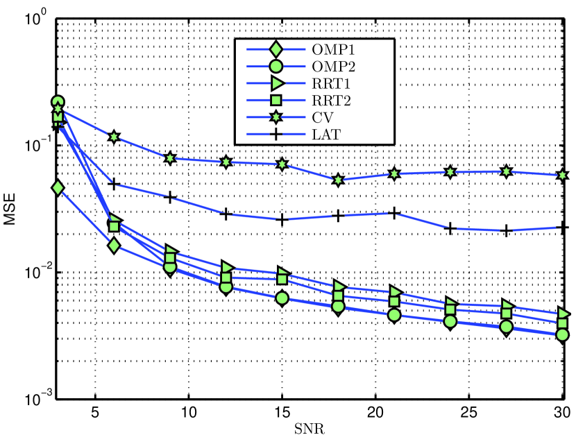
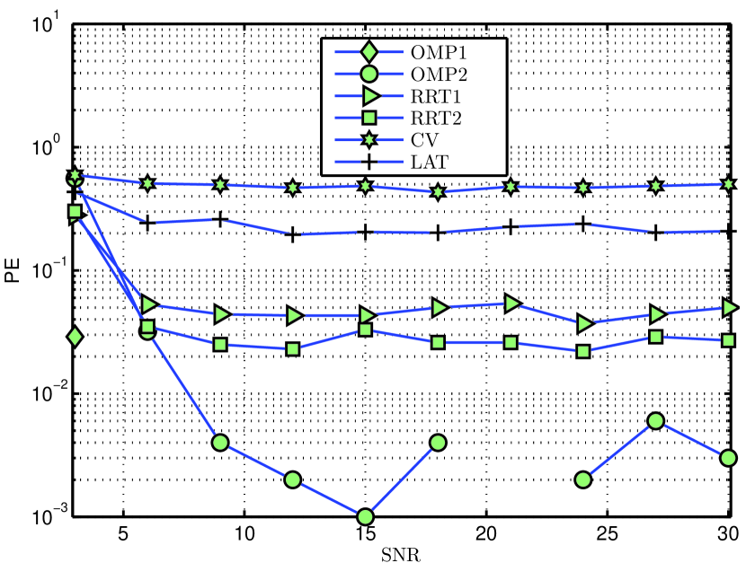
Refer to caption
Refer to caption
Figure 9: MSE and PE performances in matrix model 1.
Refer to caption
Refer to caption
Figure 10: MSE and PE performances in matrix model 2.
Refer to caption
Refer to caption
Figure 11: MSE and PE performances in matrix model 3.

References

  • Arlot etย al. (2010) Arlot, Sylvain, Celisse, Alain, etย al. A survey of cross-validation procedures for model selection. Statistics surveys, 4:40โ€“79, 2010.
  • Askitis (2016) Askitis, Dimitris. Asymptotic expansions of the inverse of the beta distribution. arXiv preprint arXiv:1611.03573, 2016.
  • Atkinson & Riani (2012) Atkinson, Anthony and Riani, Marco. Robust diagnostic regression analysis. Springer Science & Business Media, 2012.
  • Bayati etย al. (2013) Bayati, Mohsen, Erdogdu, Muratย A, and Montanari, Andrea. Estimating lasso risk and noise level. In Advances in Neural Information Processing Systems, pp.ย 944โ€“952, 2013.
  • Belloni etย al. (2011) Belloni, Alexandre, Chernozhukov, Victor, and Wang, Lie. Square-root lasso: pivotal recovery of sparse signals via conic programming. Biometrika, 98(4):791โ€“806, 2011.
  • Cai & Wang (2011) Cai, Tย Tony and Wang, Lie. Orthogonal matching pursuit for sparse signal recovery with noise. IEEE Transactions on Information theory, 57(7):4680โ€“4688, 2011.
  • Candes & Tao (2007) Candes, Emmanuel and Tao, Terence. The Dantzig selector: Statistical estimation when p is much larger than n. The Annals of Statistics, pp.ย  2313โ€“2351, 2007.
  • Chichignoud etย al. (2016) Chichignoud, Michaรซl, Lederer, Johannes, and Wainwright, Martinย J. A practical scheme and fast algorithm to tune the lasso with optimality guarantees. Journal of Machine Learning Research, 17(231):1โ€“20, 2016.
  • Dai & Milenkovic (2009) Dai, W. and Milenkovic, O. Subspace pursuit for compressive sensing signal reconstruction. IEEE Transactions on Information Theory, 55(5):2230โ€“2249, May 2009.
  • Dicker (2014) Dicker, Leeย H. Variance estimation in high-dimensional linear models. Biometrika, 101(2):269โ€“284, 2014.
  • Dicker & Erdogdu (2016) Dicker, Leeย H and Erdogdu, Muratย A. Maximum likelihood for variance estimation in high-dimensional linear models. In Artificial Intelligence and Statistics, pp.ย  159โ€“167, 2016.
  • Elad (2010) Elad, Michael. Sparse and Redundant Representations: From Theory to Applications in Signal and Image Processing. Springer, 2010.
  • Fan etย al. (2012) Fan, Jianqing, Guo, Shaojun, and Hao, Ning. Variance estimation using refitted cross-validation in ultra high dimensional regression. Journal of the Royal Statistical Society: Series B (Statistical Methodology), 74(1):37โ€“65, 2012.
  • Fletcher & Rangan (2012) Fletcher, A.ย K. and Rangan, S. Orthogonal matching pursuit: A Brownian motion analysis. IEEE Transactions on Signal Processing, 60(3):1010โ€“1021, March 2012.
  • Jin & Rao (2010) Jin, Y. and Rao, B.ย D. Algorithms for robust linear regression by exploiting the connection to sparse signal recovery. In Proc. ICAASP, pp.ย  3830โ€“3833, March 2010. doi: 10.1109/ICASSP.2010.5495826.
  • Liu etย al. (2017) Liu, C., Fang, Y., and Liu, J. Some new results about sufficient conditions for exact support recovery of sparse signals via orthogonal matching pursuit. IEEE Transactions on Signal Processing, 65(17):4511โ€“4524, Sept 2017.
  • Mallat & Zhang (1993) Mallat, Stรฉphaneย G and Zhang, Zhifeng. Matching pursuits with time-frequency dictionaries. IEEE Transactions on signal processing, 41(12):3397โ€“3415, 1993.
  • Meinshausen & Bรผhlmann (2010) Meinshausen, Nicolai and Bรผhlmann, Peter. Stability selection. Journal of the Royal Statistical Society: Series B (Statistical Methodology), 72(4):417โ€“473, 2010.
  • Mitra etย al. (2010) Mitra, K., Veeraraghavan, A., and Chellappa, R. Robust regression using sparse learning for high dimensional parameter estimation problems. In IEEE International Conference on Acoustics, Speech and Signal Processing, pp.ย  3846โ€“3849, March 2010.
  • Mitra etย al. (2013) Mitra, K., Veeraraghavan, A., and Chellappa, R. Analysis of sparse regularization based robust regression approaches. IEEE Transactions on Signal Processing, 61(5):1249โ€“1257, March 2013.
  • Mousavi etย al. (2013) Mousavi, Ali, Maleki, Arian, and Baraniuk, Richardย G. Parameterless optimal approximate message passing. arXiv preprint arXiv:1311.0035, 2013.
  • Pati etย al. (1993) Pati, Yagyenshย Chandra, Rezaiifar, Ramin, and Krishnaprasad, Perinkulamย Sambamurthy. Orthogonal matching pursuit: Recursive function approximation with applications to wavelet decomposition. In Signals, Systems and Computers, 1993. 1993 Conference Record of The Twenty-Seventh Asilomar Conference on, pp.ย  40โ€“44. IEEE, 1993.
  • Ravishanker & Dey (2001) Ravishanker, Nalini and Dey, Dipakย K. A first course in linear model theory. CRC Press, 2001.
  • Rousseeuw & Leroy (2005) Rousseeuw, Peterย J and Leroy, Annickย M. Robust regression and outlier detection, volume 589. John wiley & sons, 2005.
  • Tibshirani (1996) Tibshirani, Robert. Regression shrinkage and selection via the lasso. Journal of the Royal Statistical Society. Series B (Methodological), pp.ย  267โ€“288, 1996.
  • Tropp (2004) Tropp, Joelย A. Greed is good: Algorithmic results for sparse approximation. IEEE Transactions on Information theory, 50(10):2231โ€“2242, 2004.
  • Tropp (2006) Tropp, Joelย A. Just relax: Convex programming methods for identifying sparse signals in noise. IEEE transactions on information theory, 52(3):1030โ€“1051, 2006.
  • Tropp & Gilbert (2007) Tropp, Joelย A and Gilbert, Annaย C. Signal recovery from random measurements via orthogonal matching pursuit. IEEE Transactions on Information Theory, 53(12):4655โ€“4666, 2007.
  • Wang (2015) Wang, J. Support recovery with orthogonal matching pursuit in the presence of noise. IEEE Transactions on Information Theory, 63(21):5868โ€“5877, Nov 2015.
  • Wang etย al. (2016) Wang, Xiangyu, Dunson, David, and Leng, Chenlei. No penalty no tears: Least squares in high-dimensional linear models. In International Conference on Machine Learning, pp.ย 1814โ€“1822, 2016.
  • Wen etย al. (2016) Wen, J., Zhou, Z., Wang, J., Tang, X., and Mo, Q. A sharp condition for exact support recovery of sparse signals with orthogonal matching pursuit. In Proc. ISIT, pp.ย  2364โ€“2368, July 2016.
  • Wen etย al. (2017) Wen, Jinming, Wang, Jian, and Zhang, Qinyu. Nearly optimal bounds for orthogonal least squares. IEEE Transactions on Signal Processing, 65(20):5347โ€“5356, 2017.
  • Yang & deย Hoog (2015) Yang, Mingrui and deย Hoog, Frank. Orthogonal matching pursuit with thresholding and its application in compressive sensing. IEEE Transactions on Signal Processing, 63(20):5479โ€“5486, 2015.
  • Zou & Hastie (2005) Zou, Hui and Hastie, Trevor. Regularization and variable selection via the elastic net. Journal of the Royal Statistical Society: Series B (Statistical Methodology), 67(2):301โ€“320, 2005.