Driven Widom-Rowlinson lattice gas

Abstract

In the Widom-Rowlinson lattice gas, two particle species (A, B) diffuse freely via particle-hole exchange, subject to both on-site exclusion and prohibition of A-B nearest-neighbor pairs. As an athermal system, the overall densities are the only control parameters. As the densities increase, an entropically driven phase transition occurs, leading to ordered states with A- and B-rich domains separated by hole-rich interfaces. Using Monte Carlo simulations, we analyze the effect of imposing a drive on this system, biasing particle moves along one direction. Our study parallels that for a driven Ising lattice gas – the Katz-Lebowitz-Spohn (KLS) model, which displays atypical collective behavior, e.g., structure factors with discontinuity singularities and ordered states with domains only parallel to the drive. Here, other novel features emerge, including structure factors with kink singularities (best fitted to $\left|q\right|$), maxima at non-vanishing wavevector values, oscillating correlation functions, and ordering into multiple striped domains perpendicular to the drive, with a preferred wavelength depending on density and drive intensity. Moreover, the (hole-rich) interfaces between the domains are statistically rough (whether driven or not), in sharp contrast with those in the KLS model, in which the drive suppresses interfacial roughness. Defining a novel order parameter (to account for the emergence of multistripe states), we map out the phase diagram in the density-drive plane and present preliminary evidence for a critical phase in this driven lattice gas.

I Introduction

Driven lattice gases have played a central role in far-from-equilibrium thermodynamics and statistical mechanics, in particular in the study of phase transitions schmittmann-zia ; marro and steady-state thermodynamics (SST) ST . In this context, most studies have focussed on the lattice gas with attractive nearest-neighbor (NN) interactions pioneered by Katz, Lebowitz, and Spohn KLS (KLS). In equilibrium, this model is the lattice gas version of the Ising model LeeYang . Under a drive favoring particle motion along one axis (and suppressing motion in the opposite sense), the KLS model exhibits a variety of remarkable collective behaviors schmittmann-zia ; marro , such as generic long-range correlations LRC ; Onuki79 ; Onuki81 ; Kirkpatrick16 , ‘negative response’ ZiaPM , non-Ising critical properties JSLC , anisotropic phase separation KLS , and anomalous interfacial fluctuations leung88 ; InterfaceCorr . More recently, it has been extensively studied in connection with the difficulties in formulating a zeroth law of thermodynamics for systems driven into steady states far from equilibrium pradhan ; sst1 ; sst3 . Another model of interest is the driven lattice gas with NN exclusion (NNE lattice gas) drnne , which exhibits a complex pattern of phase ordering and jamming, and has also proved useful in efforts to define a nonequilibrium chemical potential sst2 . The NNE lattice gas is an athermal model exhibiting a phase transition to sublattice ordering. While athermal models are convenient in that they involve only a single effective parameter (the dimensionless chemical potential $\mu^{\ast}=\mu/k_{B}T$), the NNE lattice gas does not exhibit macroscopically distinguishable phases. An athermal model that does exhibit phase separation is the lattice Widom-Rowlinson (WR) model or Widom-Rowlinson lattice gas (WRLG) wrlg . It is likely the simplest model with purely repulsive interactions to undergo phase separation. This study is devoted to a driven WRLG.

The equilibrium WRLG was introduced in wrlg , as a discrete-space version of the original (continuous-space) Widom-Rowlinson model WR70 ; RW82 . Each site may be vacant, or occupied by a particle belonging to species A or species B. Nearest-neighbor A-B pairs are prohibited, as is multiple occupancy of a site. (The latter restriction departs from the original, continuous-space WR model, in which particles belonging to the same species do not interact at all.) In wrlg it is shown that the WRLG (with equal densities of A and B particles, $\rho_{A}=\rho_{B}\equiv\rho/2$) exhibits a continuous phase transition between a disordered, low-density phase and coexisting A- and B-rich phases at a critical density $\rho_{c}$. Best estimates for the critical density are 0.618(1) and 0.3542(1) on the square and simple cubic lattices, respectively. (Figures in parentheses denote statistical uncertainties.) Results on scaling behavior wrlg support an Ising-like critical point, as expected on grounds of symmetry. Subsequent studies of the WRLG have focussed on multi-species versions Nielaba-Lebowitz . Here we study the driven WRLG: as in the KLS model, and the driven NNE lattice gas, particle motion is favored along one direction, and suppressed in the opposite sense, as if an electric or other external field were acting on the particles. To model a nonequilibrium steady state, it is essential that the system have periodic boundaries along the drive direction. (For impenetrable boundaries the system corresponds to an equilibrium fluid subject to a simple linear gravitational potential.)

In the NNE lattice gas above the critical density, the sublattice-ordered phases are equivalent under a unit translation in the $x$ or $y$ direction, whereas the symmetry connecting the A- and B-rich phases in the WRLG is global exchange of A and B particles. In the driven NNE lattice gas with first- and second-neighbor hopping (the model studied by Szolnoki and Szabo, szolnoki-szabo02 ), particles are free to hop between sublattices, so there is global sublattice ordering rather than spatial separation into two phases; in this case no stripe pattern is observed.

In the single-component lattice gas with finite repulsive NN interactions, (equivalent in equilibrium to the antiferromagnetic Ising model), the drive destroys sublattice ordering szabo94 ; szabo96 . For infinite NN repulsion, i.e., the nearest-neighbor exclusion (NNE) model, phase separation under a drive is possible, as well as formation of dynamically arrested regions, if the dynamics allows NN hopping only drnne . Including hopping to second neighbors changes the phase behavior: instead of separation into high- and low-density regions, there is a continuous, Isinglike transition to a phase with sublattice ordering, as in equilibrium szolnoki-szabo02 . In the present work, the dynamics includes both NN and second-neighbor hopping.

There are two principal motivations for studying the driven WRLG. First, aside from the examples already cited, not many driven systems exhibiting phase separation have been examined in detail; the lack of attractive interactions leads to a very different sort of phase ordering under a drive, as compared with the KLS model. In this context, we should mention that the WRLG is a spin-1 or 3-state system, a class that includes well known systems such as the Potts Potts and Blume-Emery-Griffiths BEG models. Some driven 3-state models have been investigated previously Threestate , but none display the novel properties of the system we present here. Second, it is valuable to have further examples of model systems for testing SST.

There are two main foci in the present work: anomalous correlations (even in the disordered phase) and remarkably rich varieties of phase segregated order. Our principal source of information is Monte Carlo simulation of the model on the square lattice, which we complement with simple mean-field theory approaches. The first issue is best displayed in terms of the structure factor $S(q_{||},q_{\perp})$, with the subscripts denoting wavevector components along, and perpendicular to, the drive. In addition to displaying a discontinuity singularity at the origin [$S(q_{||}\rightarrow 0,0)\neq S(0,q_{\perp}\rightarrow 0)$] as observed in similar driven diffusive systems Huang93 ; Zia95 ; Korniss97 ; Praestgaard00 ; Vidigal07 ; Greulich08 , $S(q_{||}\rightarrow 0,0)$ exhibits a kink singularity, best fitted to $\left|q_{||}\right|$! This novel feature is accompanied by a maximum of $S(q_{||},0)$ located at some non-vanishing $q_{||}$ value, associated with periodic correlations of composition fluctuations along the drive direction. Let us emphasize that these properties are present even at low densities (for which the composition is spatially uniform), in stark contrast to the familiar, analytic, Ornstein-Zernike form $S(q_{||},0)\propto 1/(\tau+q_{||}^{2})$. Under the drive, composition variations are characterized by a preferred wavelength $\lambda(\rho,p)$, where $p$ denotes the intensity of the drive. The second focus is a phase diagram in the density-drive plane, as we report the emergence of multiple stripes of A- and B-rich phases [of wavelength $\lambda(\rho,p)$], oriented perpendicular to the drive! By contrast, in the KLS model, the particle-rich (or hole-rich) regions form a single stripe parallel to the drive (especially in systems with $O\left(1\right)$ aspect ratios). As in the KLS model, long-lived metastable states are observed as control parameters are changed across phase boundaries, a phenomenon reminiscent of hysteresis.

The remainder of this paper is organized as follows. In the next section we define the model. In Sec. III we examine the low-density, disordered phase, and discuss mean-field and field-theoretic approaches. Sec. IV reports our results for local and global ordering, correlations in the ordered phase, and interface roughness, followed by a summary and discussion of our findings in Sec. V .

II Model

The WRLG is defined on a lattice of $L^{d}$ sites, each of which may be empty or occupied by a particle of type A or of type B; multiple occupancy is forbidden. It is convenient to introduce occupation variables $\sigma_{i}=0$, $1$, or $-1$ for site $i$ vacant, occupied by an A particle, or occupied by a B particle, respectively. To model the NN repulsion, if $\sigma_{i}=\pm 1$, none of its nearest neighbors may have $\sigma=\mp 1$. In equilibrium, the model may be studied in the canonical ensemble, i.e., with fixed numbers of A and B particles, $N_{A}$ and $N_{B}$, respectively, or in the grand canonical ensemble, in which the associated chemical potentials, $\mu_{A}^{\ast}$ and $\mu_{B}^{\ast}$ are fixed. Here we limit our attention to the case of square lattice ($d=2$). Thus, a site is labeled by integers $\left(n_{x},n_{y}\right)\in$ $\left(\left[1,L_{x}\right],\left[1,L_{y}\right]\right)$, while $\sigma_{i}$ is denoted by $\sigma\left(\vec{x}\right)$. Unless explicitly noted otherwise, our study focuses on systems with $L_{x}=L_{y}=L$. For simplicity, we focus on systems with fixed $N_{A}=N_{B}=N$, and choose the main control parameter to be the overall density: $\rho=2N/\left(L_{x}L_{y}\right)$.

It is well to recall that the equilibrium thermodynamics of athermal systems is determined exclusively by maximization of entropy, subject to whatever constraints apply. Thus phase separation in the WR model occurs at densities high enough that the configurational entropy of the phase-separated, inhomogeneous system is higher than that of a homogenous one. As in the freezing of the hard-sphere fluid, a higher entropy is associated with a nominally more ordered phase because the disordered phase possesses relatively few configurations, due to excluded-volume constraints. To what extent such considerations apply to driven athermal systems is an open question: under a drive, the probability distribution is no longer uniform on configuration space, and the very definition of a thermodynamic entropy is in general unclear.

The driven WRLG is a stochastic process with a Markovian dynamics defined via a set of transition rates $w(\mathcal{C}^{\prime},\mathcal{C})$, from configuration $\mathcal{C}$ (i.e., the set $\left\{\sigma_{i}\right\}$) to configuration $\mathcal{C}^{\prime}$. Transitions occur via single-particle hopping, so that for $w(\mathcal{C}^{\prime},\mathcal{C})$ to be nonzero, configurations $\mathcal{C}$ and $\mathcal{C}^{\prime}$ must differ by the exchange of a particle-hole pair. Specifically, each particle attempts to hop to a first or second neighbor, that is, a displacement of $\left(\Delta n_{x},\Delta n_{y}\right)$ with $\Delta n_{x}$, $\Delta n_{y}\in\{-1,0,1\}$ (excluding the no-hop case $\Delta n_{x}=\Delta n_{y}=0$). Any hopping move that results in a configuration satisfying the prohibition against NN A-B pairs is accepted. The attempt rates are parameterized in terms of $p\in[-1,1]$ (propensity to move along $+x$) and $a\in[0,1]$ (tendency to leave $x$ unchanged):

$$w(\Delta n_{x},\Delta n_{y})=\left\{\begin{array}[]{ll}\frac{(1\!-\!a)(1\!\pm\!p)}{6},\;\;\Delta n_{x}=\pm 1,\text{ any }\Delta n_{y}&\\ \frac{a}{2},\;\;\;\;\;\;\;\;\;\;\;\;\Delta n_{x}=0,\Delta n_{y}=\pm 1&\\ 0,\;\;\;\;\;\;\;\;\;\;\;\;\Delta n_{x}=0=\Delta n_{y}&\end{array}\right.\,.$$ (1)

For $p=0$ and $a<1$, detailed balance is satisfied, and the stationary distribution of the Markov process corresponds to the equilibrium distribution, i.e., all allowed configurations equally likely. The hopping rates are isotropic for $p=0$ and $a=1/4$. (The special case of $a=1$, in which particles are restricted a given column, is not considered here.) As $p$ is varied from zero to unity, the process interpolates from a case with symmetric hopping in $x$ (equilibrium) to one with maximal asymmetry, with no hopping in the $-x$ direction. We consider a dynamics with next-nearest-neighbor as well as nearest-neighbor hopping to avoid the possibility of nongeneric patterns or dynamic arrest associated with a restriction to NN hopping szolnoki-szabo02 , and because an extended set of hopping moves favors ergodicity. Our choice of equal hopping rates for jumps with the same value of $\Delta n_{x}$ is motivated by simplicity. In the simulation studies reported here, we set $a=0$ and only comment on some runs with $a=1/4$.

II.1 Simulations

We perform Monte Carlo (MC) simulations the driven WRLG on the square lattice, using rectangular systems of $L_{x}\times L_{y}$ sites with periodic boundaries in both directions. Unless otherwise noted, we use $L_{x}=L_{y}=L$, with $L$ ranging from 30 to 400. We count one MC step as $N$ attempted particle moves. Studies of stationary properties use $2-14\times 10^{7}$ MC steps, preceded by an initial period of $10^{7}$ MC steps, which we found to be sufficient for relaxation. Averages and uncertainties (standard deviation of the mean) are calculated over 10-30 independent realizations.

III Anomalies in the homogeneous phase: Singular structure factors and correlations

If the density $\rho$ is sufficiently low, the WRLG remains homogeneous whether driven or not. Simulations of the equilibrium case show this disordered phase to prevail for $\rho<$ $\rho_{c}\simeq 0.618\left(1\right)$. As the drive parameter $p$ is increased from zero to unity, the change in $\rho_{c}$ is rather modest, attaining a value of about $0.76(1)$ for $p=1$. By contrast, the critical temperature of the driven KLS model is found to increase by as much as $40\%$ (in $d=2$) from equilibrium KLS . In this section, we focus our attention on the low-density disordered state, in which we find anomalies in the correlation functions and structure factors, beyond those observed in the KLS system.

III.1 Simulation studies of the structure factor and correlation functions

One standard way to characterize collective behavior is through correlation functions ($G$) and their Fourier transforms, the structure factors ($S$). For simplicity, we consider only equal-time, two-point correlations; since there are two species of particles, these are $2\times 2$ matrices. Instead of the densities of the two particle species, $\rho_{A,B}\left(\vec{x}\right)$, symmetry guides us to consider their sum and difference, which will be referred to as “mass” and “charge” densities

$$\rho\left(\vec{x}\right) \equiv \rho_{A}\left(\vec{x}\right)+\rho_{B}\left(\vec{x}\right),$$

$$\psi\left(\vec{x}\right) \equiv \rho_{A}\left(\vec{x}\right)-\rho_{B}\left(\vec{x}\right),$$

respectively notation . While this notation is unnecessary for reporting simulation data (as they are just, respectively, $\left|\sigma\left(\vec{x}\right)\right|$ and $\sigma\left(\vec{x}\right)$ at each $\vec{x}$), it sets the stage for a field-theoretic approach, the simplest of which will be discussed below. The restrictions of our simulations correspond to the constraints $\langle\left|\sigma\left(\vec{x}\right)\right|\rangle=\rho$ and $\langle\sigma\left(\vec{x}\right)\rangle=0$.

In terms of these densities, the $2\times 2$ matrix of correlations consists of $G_{\rho\rho}$ and $G_{\psi\psi}$. The cross correlation, $G_{\rho\psi}=G_{\psi\rho}$, is the difference $G_{AA}-G_{BB}$ which vanishes (statistically) in the symmetric systems we study. For simply, we write $G_{\rho\rho,\psi\psi}$ as $G_{\rho}$ and $G_{\psi}$. In the steady state, translational invariance dictates that these are functions of $\vec{r}$, the distance between the two points in question. Thus,

$$G_{\rho}(\vec{r}) \equiv \langle\left|\sigma\left(\vec{x}\right)\right|\left|\sigma\left(\vec{x}+\vec{r}\right)\right|\rangle-\rho^{2}$$

$$G_{\psi}(\vec{r}) \equiv \langle\sigma\left(\vec{x}\right)\sigma\left(\vec{x}+\vec{r}\right)\rangle$$

are independent of $\vec{x}$; to improve statistics, we average over $\vec{x}$. When we form the covariance or connected correlation function by subtracting the associated expectations, $\left\langle\sigma\right\rangle\left\langle\sigma\right\rangle$, these $G$’s assume different values at the origin: $G_{\rho}(\vec{0})=\rho\left(1-\rho\right)$ vs. $G_{\psi}(\vec{0})=\rho$, since $\sigma^{2}\left(\vec{x}\right)=\left|\sigma\left(\vec{x}\right)\right|^{2}=\left|\sigma\left(\vec{x}\right)\right|$. Meanwhile, the sum $\sum_{\vec{r}}G(\vec{r})$ vanishes for both functions. The structure factors are the Fourier transforms

$$S\left(\vec{q}\right)=\sum_{\vec{r}}G(\vec{r})e^{i\vec{q}\cdot\vec{r}}$$ (2)

By averaging over $\vec{x}$ to obtain $G$, we also have, e.g., $S_{\psi}=L^{-2}\sum_{\vec{x},\vec{r}}\langle\sigma\left(\vec{x}\right)\sigma\left(\vec{x}+\vec{r}\right)\rangle e^{i\vec{q}\cdot\vec{r}}=\sum_{\vec{x},\vec{x}^{\prime}}\langle\sigma\left(\vec{x}\right)e^{-i\vec{q}\cdot\vec{x}}\sigma\left(\vec{x}^{\prime}\right)e^{i\vec{q}\cdot\vec{x}^{\prime}}\rangle$, which is $L^{-2}$ times $\left\langle\left|\sum_{\vec{x}}\sigma\left(\vec{x}\right)e^{i\vec{q}\cdot\vec{x}}\right|^{2}\right\rangle$, the average over a run of the power spectrum beam , of each configuration $\sigma\left(\vec{x}\right)$. Finally, the constraints on $G$ translate into $\sum_{\vec{q}}S_{\rho}\left(\vec{q}\right)=\rho\left(1-\rho\right)L^{2}$, $\sum_{\vec{q}}S_{\psi}\left(\vec{q}\right)=\rho L^{2}$, and $S_{\rho,\psi}\left(\vec{0}\right)=0$. These serve as useful checks on simulation data. In addition, the last constraint implies that, unlike the ordinary Ising model, $S\left(\vec{0}\right)$ cannot serve as a susceptibility-like quantity for detecting a second-order critical point. Instead, our $S$ assumes its maximum value at some non-vanishing $\vec{q}$. The maximum value behaves like the susceptibility of ferromagnetic systems, i.e., remaining finite (as $L\to\infty$) in the disordered phase. For large enough $\rho$, as we report in Sec. IV, this value diverges as $L^{2}$ and so is an ideal candidate for an order parameter. If the transition turns out to be critical (i.e., behaves much like second-order transitions in equilibrium statistical systems), then the large-$L$ behavior of $S(q_{max})$ can provide us with a critical exponent.

In general, the two-point equal-time correlation, $G\left(\vec{r}\right)$, must be symmetric under parity ($\vec{r}\Leftrightarrow-\vec{r}$) and statistically symmetric under the reflections ($x\Leftrightarrow-x$ and $y\Leftrightarrow-y$). In equilibrium, there is an additional symmetry, the $x\Leftrightarrow y$ exchange (especially for samples with $L_{x}=L_{y}$). By contrast, the drive should break the last symmetry. Thus, in addition to studying $G$ and $S$ in the whole plane, we will pay special attention to the specific directions along and perpendicular to the drive. In particular, we will consider, e.g.,

$$G_{\psi||}(r)\equiv\langle\sigma\left(\vec{x}\right)\sigma\left(\vec{x}+r\hat{x}\right)\rangle;~{}~{}G_{\psi\perp}(r)\equiv\langle\sigma\left(\vec{x}\right)\sigma\left(\vec{x}+r\hat{y}\right)\rangle$$ (3)

and

$$S_{\psi||}(k)\equiv S_{\psi}\left(q_{||}=k,0\right);~{}~{}S_{\psi\perp}(k)\equiv S_{\psi}\left(0,q_{\perp}=k\right)$$ (4)

Let us call attention to the different roles played by the quantities $\vec{q}$ and $k$. The former is a wave vector, being the conjugate to the vector $\vec{x}$, with components $\left(q_{||},q_{\perp}\right)$. The latter is a wavenumber, measuring the magnitude of $\vec{q}$ along one of two axes, in the same spirit that $r$ is the magnitude of $\vec{x}$ along one of the axes. Thus, $S_{\psi||}(k)$ and $G_{\psi||}(r)$ are not simply related to each other by Fourier transforms. Instead, $S_{\psi||}\left(k\right)$ is the transform associated with the average charge density over a column $\bar{\psi}_{||}\left(x\right)\equiv L^{-1}\sum_{y}\sigma\left(x,y\right)$ and its correlation function ${C_{\psi||}(r)=\langle\bar{\psi}_{||}\left(x\right)\bar{\psi}_{||}\left(x+r\right)\rangle}$. Similarly, we can define the transverse counterparts: $\bar{\psi}_{\bot}\left(y\right)\equiv L^{-1}\sum_{x}\sigma\left(x,y\right)$ and $C_{\psi\bot}\left(r\right){=}{\langle\bar{\psi}_{||}\left(y\right)\bar{\psi}_{||}\left(y+r\right)\rangle}$. (Of course, translational invariance of the steady state provides the $x$ or $y$ independence of the $C$’s.) We will not discuss these functions explicitly below, but focus on the $S$’s, as the latter contain the same information about the system, displayed in a better form.

With this setup, let us turn to the remarkable behavior revealed by simulations. For simplicity, we focus mainly on $\psi$ and occasionally mention results for $\rho$. Thus, we drop the subscripts on $G_{\psi}$ and $S_{\psi}$ as well. Considering first the $S$’s, we report results found mainly in a $a=0,p=1,\rho=0.4,L=100$ system. The reason for this choice is that the novel and most interesting features are best displayed here.

In Fig. 1, we show $S\left(\vec{q}\right)$ and immediately notice a feature quite distinct from the structure factor of the KLS model, namely, the presence of “twin peaks.” Despite being in the disordered, homogeneous phase, such prominent structures represent a major deviation from the simple Lorentzian $1/(\tau+\vec{q}^{2})$ form of the equilibrium WRLG, as well as the discontinuity singularity at ${\vec{q}}=0$ found in the KLS model KLS ; schmittmann-zia , $\left(\nu_{x}q_{x}^{2}+\nu_{y}q_{y}^{2}\right)/\left(\tau_{x}q_{x}^{2}+\tau_{y}q_{y}^{2}+O\left(q^{4}\right)\right)$. While the data show $S_{\bot}\left(k\right)$ decreasing monotonically as $k$ increases from zero, $S_{||}\left(k\right)$ rises to a maximum at wavenumber $9$ before dropping. Such a peak is indicative of a preferred wavelength induced by the drive: $\lambda\equiv 2\pi/k_{\max}$.

Figure 1: (Color online) Structure factor for $\rho=0.4$, $p=1$, $a=0$, system size $L=100$. Left: three-dimensional surface plot; right: contour plot.

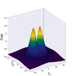
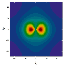
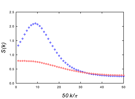
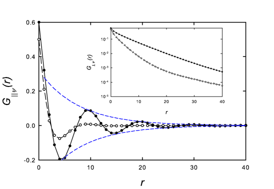
To be more confident of this unusual behavior in $S_{||}\left(k\right)$, we considered finite size effects, illustrated in Fig. 2. As the figure shows, the data points for $L=50$ and $200$ fall well within statistical errors of the $L=100$ sample, so that, for this density and drive, the thermodynamic limit is well represented by the $L=100$ system. Thus, we see that the small-$k$ region of $const./S_{||}$ is well fit by $\tau+\left(\left|k\right|-k_{\max}\right)^{2}$. Alternatively, we can write $S_{||}\left(k\right)\propto 1/\left[1+\left(\left|k\right|-k_{\max}\right)^{2}\xi_{||}^{2}+O\left(k^{4}\right)\right]$, which displays the presence of another length, $\xi_{||}$, a candidate for a “correlation length.” Note that $S_{||}\left(k\right)$ must be even in $k$, as the equal-time two-point correlations in the steady state must be even in $x$. Thus, the presence of peaks symmetric about $k=0$ is inevitable. Although, in principle, $\left(k^{2}-k_{\max}^{2}\right)^{2}$ satisfies these symmetry conditions, Fig. 3 (diamonds) shows that there is, without doubt, a kink singularity ($\propto\left|k\right|$) at $k=0$, so that the quadratic expression proposed above is a much better fit to $1/S_{||}$. In this regard, though a kink singularity is not necessary to generate period structures, the observed oscillations are best modeled by one. The inset of Fig. 2 shows that the data for $1/S_{||}$ are well fit by a quadratic expression, $0.475+1.11\left(\left|k\right|-k_{\max}\right)^{2}$, with

$$k_{\max}\cong 0.56;~{}~{}\lambda\cong 11.$$

Figure 2: (Color online) Reciprocal of structure factor for system sizes $L=50$ (circles), 100 ($+$ signs) and 200 (dots); other parameters as in Fig. 1. Inset: data for $L=100$ (points) compared with quadratic fit (curve) to 17 points nearest the minimum.

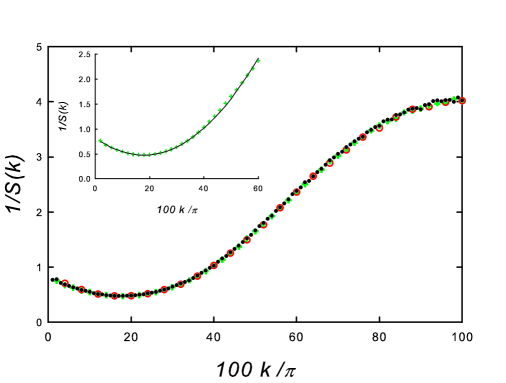
This form implies that $\xi_{||}\simeq\sqrt{1.11/0.475}\simeq 1.5$. Meanwhile, Fig. 3 (circles) shows that $S_{\bot}$ is consistent with the ordinary Lorenztian form. Of course, the drive induces anisotropy, so that $\xi_{\bot}\neq\xi_{||}$ in general. As in the KLS model, only one of the correlation lengths, $\xi_{||}$, diverges as the critical point is approached, as discussed below. Our best phenomenological estimate for the structure factor (for small $\vec{k}$, for this sample) is

$$S\left(\vec{q}\right)=\frac{\nu_{||}q_{||}^{2}+\nu_{\bot}q_{\bot}^{2}}{\tau_{||}q_{||}^{2}+\tau_{\bot}q_{\bot}^{2}+q_{||}^{2}\left(\left|q_{||}\right|-k_{\max}\right)^{2}+2\gamma_{\times}q_{||}^{2}q_{\bot}^{2}+\gamma_{\bot}q_{\bot}^{4}+...}$$ (5)

While such a form may seem unusual, it is based on a stochastic field theory which has proven successful in describing the KLS model JSLC (the numerator and denominator being associated with the noise and deterministic part of a Langevin equation for the density field). The main novel feature here is the presence of $k_{\max}$. (We also note that at the critical point, it is $\tau_{\perp}$ that vanishes in KLS, whereas $\tau_{||}$ vanishes in the present case.) To retrieve the undriven case, we need only set $k_{\max}=0$, $\nu_{||}=\nu_{\bot}=\gamma_{\times}=\gamma_{\bot}=1$, and $\tau_{||}=\tau_{\bot}$. Though this form most likely has limited validity (e.g., the presence of the singular expression $\left|q_{||}\right|$ for all $q_{\bot}$), there is no good theoretical basis for us to propose additional terms at present. Thus, we will discuss the salient features associated with this expression.

Figure 3: (Color online) Structure factors $S(k_{x},0)$ (diamonds) and $S(0,k_{y})$ (circles) for parameters as in Fig. 1.

Recall that, in our notation, $S_{||}\left(k\right)$ is given by Eq. (5) with $q_{||}=k$ and $q_{\bot}=0$, while $S_{\bot}\left(k\right)$ is obtained when we set $q_{||}=0$ and $q_{\bot}=k$. As in the KLS model, the discontinuity singularity is induced by violation of detailed balance JSLC and displayed through

$$\Delta\equiv\frac{\nu_{||}}{\tau_{||}+k_{\max}^{2}}-\frac{\nu_{\bot}}{\tau_{\bot}}\neq 0$$

Considering the points nearest the origin (for this system size), we have $S\left(\pi/50,0\right)\simeq 1.32$ and $S\left(0,\pi/50\right)\simeq 0.78$ (Fig. 3), so that $\Delta\simeq 0.54$. This singularity is manifested in configuration space by $G\left(\vec{r}\right)$ decaying as $\left(\Delta/2\pi\right)(y^{2}-x^{2})/(x^{2}+y^{2})^{2}$ at large distancesLRC . Although such a power will dominate the ordinary exponential decay for sufficiently large $r$, the crossover will depend on the ratio of the amplitudes of the two contributions. In this case, there appears to be only a small regime ($10\lesssim r\lesssim 20$) where power laws finiteL , are found in both $G_{||}$ and $G_{\bot}$. While the data are consistent with $G_{||}$ being $-\Delta/\left(2\pi x^{2}\right)$, the case for $G_{\bot}$ appears to support the power $-3$ instead. If more extensive simulations bear out this scenario, then it will be a challenge to understand such anomalous, yet “generic” (in the sense of being present far from critical points) singularities.

Let us return to the more prominent feature, namely, the presence of a maximum at non-vanishing $q_{||}$, accompanied by the singular $\left|q_{||}\right|$ at the origin. Not surprisingly, the main consequence is oscillations in $G_{||}$, within an exponential envelope. In the $\rho=0.4$ case, $\xi_{||}\ll\lambda$, so that the oscillations implied by $\lambda$ are not easily seen. These features are however prominent at larger densities, where $\xi_{||}$ is more comparable to $\lambda$. Meanwhile, as might be expected, no oscillations are found in $G_{\bot}$. In Fig. 4 we show both $G_{||}$ and $G_{\bot}$ for systems with $\rho=0.5$ and $0.6$ (again, with $a=0$, p=1 and $L=100$). The rapid increase in $\xi_{||}$ over that for $\rho=0.4$, along with hardly any changes in $\Delta$, implies that the power-law decays in $G$ are mostly masked. To be more confident of the nature of such powers (expected or “anomalous”), we will need to perform longer simulations (for statistics) of larger systems (to open a larger window between $\xi_{||}$ and $L/2$).

Figure 4: (Color online) Main graph: $G_{||}$ for densities 0.5 (open symbols) and 0.6 (filled symbols), for $p=1$, $a=0$ and $L=100$. The dashed curves are an exponential envelope fit to the data for density $0.6$. Inset: $G_{\bot}$ for the same parameters (note semilog scale).

As shown in Fig. 2, deep in the disordered phase ($\rho=0.4$), finite-size effects appear to be minimal already for $L=O\left(100\right)$. It is clear that, for this density, there is no need to simulate larger systems to capture the essence of the prominent properties of the driven WRLG. By contrast, in the next section, we show that the maximum in $S\left(\vec{k}\right)$ increases with $\rho$, so that, for sufficiently large densities, the value does not converge as $L\rightarrow\infty$. Instead, $S_{||}\left(k_{\max}\right)$ will diverge as the system size, so that $S_{||}\left(k_{\max}\right)/L^{2}$ can serve as an order parameter, in the same spirit as $S\left(\vec{0}\right)/L^{2}$ is a measure of the (square of the) spontaneous magnetization in the non-conserved Ising model in two or more dimensions. Along these lines, we mention for comparison, the divergence of $S\left(0,2\pi/L\right)$ or $S\left(2\pi/L,0\right)$ for the 2D Ising lattice gas and of $S\left(0,2\pi/L\right)$ alone for the KLS model. Different from these examples, here $S$ diverges at an $L$-independent wave-vector $\left(k_{\max},0\right)$ over a sizable region of the $\rho$-$p$ plane.

III.2 Discrete mean-field theory and its continuum limit

In this subsection, we present the simplest theoretical description, as the first, small step towards a more comprehensive theory. The idea here is to consider two continuous variables at each discrete site, each corresponding to the average occupation by the two species: $\rho_{A,B}\left(\vec{x},t\right)$. Next, we postulate the simplest gain/loss terms for the change in $\rho_{A,B}$ in a single time step. Instead of writing every term here, let us illustrate with just one example: the loss to $\rho_{A}\left(\vec{x},t\right)$ due to $A$ particles hopping along $x$ (the $t$ argument is dropped for simplicity):

$$\frac{\left(1\!-\!a\right)\left(1\!+\!p\right)}{6}\rho_{A}\left(x,y\right)h\left(x\!+\!1,y\right)\left[1\!-\!\rho_{B}\left(x\!+\!1,y\!+\!1\right)\right]\left[1\!-\!\rho_{B}\left(x\!+\!1,y\!-\!1\right)\right]\left[1\!-\!\rho_{B}\left(x\!+\!2,y\right)\right]+$$ (6)

$$+\frac{\left(1\!-\!a\right)\left(1\!-\!p\right)}{6}\rho_{A}\left(x,y\right)h\left(x\!-\!1,y\right)\left[1\!-\!\rho_{B}\left(x\!-\!1,y\!+\!1\right)\right]\left[1\!-\!\rho_{B}\left(x\!-\!1,y\!-\!1\right)\right]\left[1\!-\!\rho_{B}\left(x\!-\!2,y\right)\right]$$ (7)

Here, $h\equiv 1\!-\!\rho_{A}\!-\!\rho_{B}$ is the density of holes. The rest of the analysis is straightforward, though quite tedious. It is clear that such terms would be exact if we had written the averages of the products of the appropriate $\sigma$s. In a mean-field (MF) approximation, these are replaced by the appropriate products of the averages, e.g., $\left\langle\sigma\left(1-\left|\sigma\right|\right)\right\rangle\rightarrow(\rho_{A}-\rho_{B})h$. Beyond the site approximation pursued here, a (generally) more reliable (and complicated) approach is the pair approximation, which treats nearest-neighbor two-site joint probabilities as the basic elements marro . Although we plan to implement the pair approximation in future work, it seems possible that only more sophisticated theories will be able to capture the periodic structure observed under a drive.

Since $\rho_{A}\left(\vec{x},t\right)$ is a conserved density, the gain and loss terms are necessarily representable in terms of divergences of currents. Identifying the terms associated with the net hops from, say, $x$ to $x+1$, we find the leading contribution by setting both densities to be the overall value: $\rho_{A,B}=\rho/2$. This is the same approach used to find the current-density relationship $J_{KLS}\left(\rho\right)=\rho\left(1-\rho\right)$ in the KLS model. The result here is

$$J_{MF}\left(\rho\right)=\left(1-a\right)p\,\frac{\rho}{2}\left(1-\rho\right)\left(1-\frac{\rho}{2}\right)^{3}$$ (8)

where the various factors can be readily associated with those in, say, Eq. (6).

In Fig. 5, we show this $J_{MF}\left(\rho\right)$ (dashed line) and the simulation data (symbols) for a system of size $L=200$ with $a=0,p=1$, as well as $J_{KLS}\left(\rho\right)$ (dotted line) for comparison. It is remarkable how the properties of a complicated stochastic system are mostly captured (i.e., $\rho\lesssim 0.9$) by such a simple minded approach. Near the $\rho=1$ limit, we note that the data jump to follow another “branch” of the $J$-$\rho$ relationship, which is much closer to $J_{KLS}\left(\rho\right)$. This seemingly paradoxical result can also be understood, as follows. The jumps in the data are associated with “merging” transitions, where many strips merge into fewer. Eventually, the system settles into a single strip (for each species) configuration. In this limit, it is natural to regard the holes as “particles” and particles as “holes.” The idea is that only some of these “particles” are bound to interfaces which separate the $A$- and $B$-rich domains. Roughly speaking, $\rho L^{2}-2L$ of them remain mobile and are driven through the large domains of “holes,” interacting in a minimal way with the ones bound to the interfaces. Thus, we can apply $J_{KLS}$ to this system, with the density of “particles” being $\rho-2/L$ and (mobile) “holes” being $1-\left(\rho-2/L\right)$. In the large $L$ limit, such an expression reduces precisely to $\rho\left(1-\rho\right)$. Without showing it explicitly, the agreement between data and $\left(\rho-2/L\right)\left(1-\rho+2/L\right)$, with $L=200$, is excellent. The reason the current associated with single-stripe configurations lies much closer to the simple KLS prediction is that in this case the density of mobile vacancies is much nearer $1-\rho$.

Figure 5: (Color online) Current density $j$ versus particle density $\rho$ for drive parameters $p=1$ and $a=0$, system size $L=200$. Points: simulation results; solid curve: mean-field prediction, Eq. (8); dashed curve: simple mean-field prediction, $j=\rho(1-\rho)\equiv J_{KLS}$.

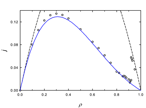
In Fig. 5, there is a range of densities (approximately $0.86\leq\rho\leq 0.87$) in which both multistripe and single-stripe configurations exist. Although the former appear to be metastable, precise determination of the associated lifetimes is left for future study. On a lattice of $L\times L$ sites, the maximum possible density is $1-L/2$. Configurations with this density are frozen, since there are then no mobile vacancies. Outside this limit, however, we do not observe jamming in the sense found in the driven NNE model with NN hopping dynamics drnne .

The next natural step in the attempt to formulate a theoretical approach is to write a continuum approximation for the discrete MF, while keeping the lowest few orders in the expansion of the displaced densities, e.g., $\rho\left(x+1\right)\rightarrow\rho\left(x\right)+\varepsilon\partial_{x}\rho+\left(\varepsilon\partial_{x}\right)^{2}\rho/2+...$. The final step is to limit our present study to the homogenous phase and consider the lowest orders in the expansion of the densities

$$\rho_{A,B}\left(\vec{x},t\right)=\frac{\rho}{2}+\phi_{A,B}\left(\vec{x},t\right)+...$$

In this manner, we obtain expressions for $\partial_{t}\phi_{A,B}\left(\vec{x},t\right)$. If we keep only the order linear in $\phi$, we will find

$$\partial_{t}\left(\begin{array}[]{c}\phi_{A}\\ \phi_{B}\end{array}\right)=\left(\begin{array}[]{cc}D&\tilde{D}\\ \tilde{D}&D\end{array}\right)\left(\begin{array}[]{c}\phi_{A}\\ \phi_{B}\end{array}\right)$$ (9)

where $D$ and $\tilde{D}$ are differential operators. Note that we have taken account of the symmetry under $A\Leftrightarrow B$ to write this form. Clearly, the sum and difference of the $\phi$ fields diagonalize this matrix. There should be no confusion if we again use the notation $\psi\left(\vec{x},t\right)$ for $\phi_{A}-\phi_{B}$. In keeping with the discussions above, we will focus on the $\psi$ equation only, though the sum, $m\left(\vec{x},t\right)\equiv\phi_{A}+\phi_{B}$, will play a role at the nonlinear level. The result of a tedious computation is, apart from the details of the coefficients, to be expected from the fact that $\psi$ is a conserved density. Thus, we find $\partial_{t}\psi$ to be the divergence of a current density, obeying the appropriate space-time symmetries:

$$\partial_{t}\psi=\left[\left(E_{1}\partial_{x}+E_{3}\partial_{x}^{3}...\right)+\left(D_{||}\partial_{x}^{2}+D_{\bot}\partial_{y}^{2}+...\right)\right]\psi$$

For clarity, we have kept the parts odd in $\partial_{x}$ (which must be absent when $p=0$) separate from those even in $\partial_{x,y}$ (which represent the diffusive parts of this equation). Thus in Fourier space $\left(\vec{q},\omega\right)$, the former set appears with $i$ and can be seen as the real part of a dispersion relation, $\omega\left(\vec{q}\right)$, which plays the role of driven transport. The imaginary part plays the role of damping, providing the sign is appropriate. From these, we have also allowed for anisotropic diffusion ($D_{||}\neq D_{\bot}$), as $p,a$ are not necessarily $0,1/4$. Of course, the various coefficients are real functions of $\rho$, $p$ and $a$, the only control parameters here. At this level, all are expected to be analytic, so that we expect the $E$’s and $D$’s to be odd and even functions, respectively, of the drive $p$. Naturally, the next step is to explore (linear) instability, by checking if any aspect of the damping vanishes. The only such occurrence is $D_{||}$ vanishing at $\rho=1/6$, independent of $p$, corresponding to the the unmixing transition in the equilibrium WRLG. Needless to say, this instability is of little relevance to our driven lattice gas. But, as a mean-field-like result, it may serve as a starting point for serious analysis.

To gain some insight into the structure factors and correlations, we must add noise terms to form a set of Langevin equations for the density fields, though these terms cannot be derived from the discrete mean-field equations above. Thus we write,

$$\partial_{t}\psi=\left[\left(E_{1}\partial_{x}+E_{3}\partial_{x}^{3}...\right)+\left(D_{||}\partial_{x}^{2}+D_{\bot}\partial_{y}^{2}+...\right)\right]\psi+\eta\left(\vec{x},t\right).$$ (10)

To account for the conservation law and possible anisotropy, we will assume that $\eta$ is delta-correlated, conserved, Gaussian noise, with zero mean and

$$\left\langle\eta\left(\vec{x},t\right)\eta\left(\vec{x}^{\prime},t^{\prime}\right)\right\rangle=-\left[N_{||}\partial_{x}^{2}+N_{\bot}\partial_{y}^{2}\right]\delta\left(\vec{x}-\vec{x}^{\prime}\right)\delta\left(t-t^{\prime}\right).$$

Here again we have allowed for anisotropy, by writing two different coefficients. As a reminder, in the undriven limit, our dynamics satisfy detailed balance, which implies $N_{||}/D_{||}=N_{\bot}/D_{\bot}$. Following standard routes pioneered by Martin-Siggia-Rose MSR , Janssen HKJ , and de Dominicis CdD , we write the dynamic functional $\mathcal{J}\left[\psi,m;\tilde{\psi},\tilde{m}\right]$ for both the original density fields and the associated response fields $\tilde{\psi},\tilde{m}$. At the quadratic level, corresponding to the linear Langevin example above, the $\psi$ and $m$ sectors decouple. The propagators and correlators (e.g., in the $\psi$ sector, the $\psi\tilde{\psi}$ and $\tilde{\psi}\tilde{\psi}$ terms) in Fourier space are, respectively, $i\left[\omega-\omega\left(\vec{q}\right)\right]+D_{||}q_{x}^{2}+D_{\bot}q_{y}^{2}+O\left(q^{4}\right)$ and $N_{||}q_{x}^{2}+N_{\bot}q_{y}^{2}$. The most general $O\left(q^{4}\right)$ terms consistent with symmetry, anisotropy, and analyticity are just $\Gamma_{||}q_{x}^{4}$, $\Gamma_{\times}q_{x}^{2}q_{y}^{2}$ and $\Gamma_{\pm}q_{y}^{4}$ . Thus, at this tree level, the equal-time correlation $G_{tree}\left(\vec{r},0\right)$ can be found easily; its transform reads,

$$S_{tree}\left(\vec{q}\right)=\frac{N_{||}q_{x}^{2}+N_{\bot}q_{y}^{2}}{D_{||}q_{x}^{2}+D_{\bot}q_{y}^{2}+O\left(q^{4}\right)}$$

While this approach may appear to be reasonable for describing the fluctuations of the homogeneous state, clearly, it fails to predict the most prominent feature: presence of a $\left|q_{x}\right|$ term and the associated maximum at $k_{\max}$. We are exploring non-linear terms in the Langevin equation (beyond quadratic in $\mathcal{J}$) and whether a simple perturbative approach can generate such a kink singularity. We conjecture that at one-loop level, a term $\propto\left|q_{||}\right|^{3}$ will emerge in the denominator, thereby justifying the form in Eq. (5). Work is in progress to examine a systematic approach, applying the Doi-Peliti formalism Doi ; Peliti ; Pert ; DPrev to the defining microscopic dynamics to derive (instead of postulating) the appropriate functional. It is our hope that results from such an analysis will provide a better description of the phenomenological form above. The success of stochastic field theory in the past is, of course, the systematic study of universal properties in critical phenomena. Assuming that the transition from the homogeneous to the inhomogeneous state(s) is continuous, we believe this line of pursuit will lead to novel fixed point(s) and universality class(es).

IV Inhomogeneous states: Phase segregation, multiple stripes, correlations, and interfacial properties

In this section we report simulation results on the ordered phase of the driven WRLG. In equilibrium, for $\rho_{A}=\rho_{B}=\rho/2$, the system exhibits separation into A- and B-rich phases above a certain critical density. We therefore begin by looking for signs of phase separation under a drive.

IV.1 Emergence of striped phases under a drive

As shown in the preceding section, under a drive, the disordered system exhibits a preferred wavelength $\lambda$ for charge density oscillations. We find that, for densities $\rho$ near the onset of phase separation, a striped pattern of wavelength $\lambda$ appears, as is evident in configuration snapshots as well as quantitative measures such as the structure factor. With increasing density, $\lambda$ first decreases, attaining a minimum $\lambda_{min}$ for $\rho\simeq 0.65-0.70$, and then grows, approaching the system size $L_{x}$, as $\rho\to\rho_{max}=1-2/L_{x}$. (Recall that at least $2L_{y}$ vacancies are required to satisfy the prohibition of NN A-B pairs.) We expect that in the limit $L_{x},L_{y}\to\infty$, with fixed $L_{y}/L_{x}$ and $\rho<1$, the wavelength $\lambda$ converges to a size-independent function of the density and the drive parameters.

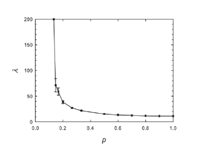
In equilibrium, of course, maximum entropy implies the minimum possible number of interfaces, so that $\lambda$ is formally infinite for zero drive. (There is, of course, no striped pattern in equilibrium.) Consistent with this, $\lambda$ grows systematically as the drive $p\to 0$. For $p=1$, 1/2, 1/3, 1/4 and 1/8, we find $\lambda_{min}$ = 10, 15, 18, 22 and 36 respectively; these data follow $\lambda\simeq C_{1}+C_{2}/p$ where $C_{1}$ and $C_{2}$ are constants.

In contrast to the KLS model, stripes of distinct phases orient perpendicular to the drive, and have rough interfaces. For a wide range of densities, single-stripe configurations (i.e., $\lambda=L_{x}$) are unstable, and the steady state exhibits multiple stripes; for the system sizes investigated, single-stripe configurations do appear to be stable for higher densities (specifically, for $\rho\geq 0.83$ when $a=0$ and $p=1/3$, and for $\rho\geq 0.93$, for $a=0$ and $p=1$). These observations are illustrated for $a=0$ and $p=1/3$, in Figs. 6a and 7. For the densities shown, A- and B-rich regions are evident, organized into stripes oriented perpendicular to the drive. At the highest density shown, $\rho=0.85$, each phase occupies a single stripe, a situation that persists for systems of size $L\leq 400$. The configurations shown in Figs. 6-8 were obtained using single-stripe initial conditions (perpendicular to the drive), thus demonstrating instability toward formation of multiple stripes for $\rho\leq 0.82$.

We note that, for $\rho>\rho_{c}$ and a nonzero drive, initial configurations with A- and B-regions separated by a boundary parallel to the drive rapidly reorganize so that resulting the stripe or stripes are perpendicular to it. After a short time ($\sim 10^{3}$ MC steps) the initially flat interface develops waves which grow steadily in amplitude. When they reach a height $\sim L/2$, they reconnect via the periodic boundaries, forming stripes perpendicular to the drive. The latter are initially quite irregular, but (for sufficiently high densities) rapidly become ordered, so that the system is separated into clear bulk and interfacial regions.

Figure 6: (Color online) Typical configurations of driven Widom-Rowlinson lattice gas, system size $L=200$, parameters $a=0$ and $p=1/3$, with the drive oriented toward the right. Points of differing color denote particles of species A and B, respectively; white points denote vacant sites. Particle densities $\rho=0.7$ (a), 0.75 (b), 0.80 (c), 0.85 (d).

Figure 7: (Color online) Configuration for $L=400$, $\rho=0.85$, $a=0$ and $p=1/3$.

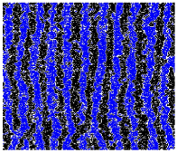
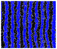
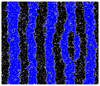
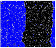
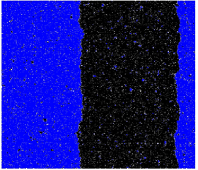
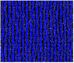
While experience with the KLS model might lead one to expect interfaces parallel to the drive, it appears that without attractive interactions there is no mechanism for stabilizing and smoothing such an interface in the driven WRLG. On the other hand, sequences of the form A0B (where 0 represents a vacant site) along the drive represent barriers, behind which particles may form a queue (and analogously for B0A sequences). Formation of queues (together with the prohibition of A-B NN pairs) may stabilize stripes perpendicular to the drive. Why many stripes of the same phase form, instead of just one, is unclear. Figure 6c provides a hint of the mechanism: a fluctuation in the boundary has allowed B particles to invade an A stripe, leading to formation of a new stripe. Multi-stripe configurations may contain defects, as is evident in Figs. 6a and 8.

Figure 8: (Color online) Configuration for $L=400$, $\rho=0.7$, $a=0$ and $p=1/3$.

IV.1.1 The preferred wavelength

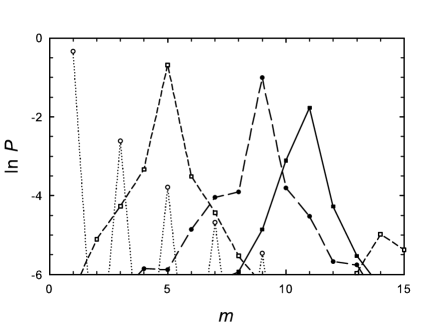
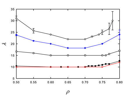
As noted above, for a nonzero drive, the structure factor $S_{||,k}$ shows a distinct maximum for a certain wavenumber, $k=2\pi m/L$, corresponding to the preferred wavelength $\lambda=L/m$. Power spectra of the columnwise charge density $\psi_{||,i}$ are particularly useful in determining $\lambda$ (see Fig. 9). The latter is a decreasing function of drive at fixed density, as shown in Fig. 10. Since the density of vacancies $1-\rho$ is complementary to the particle density, and since each stripe requires at least $2L$ vacancies for the interfaces, the number of stripes should decrease (and $\lambda$ increase) as the density approaches unity, as verified in Fig. 11. This figure also shows that the dependence of $\lambda$ on $\rho$ for different drive strengths is qualitatively similar, and that the dependence of $\lambda$ on system size is weak.

Our results for $\lambda$ derive from initial configurations (ICs) using both single and multiple stripes. For densities in the range $0.5\leq\rho<0.8$, the different ICs yield consistent results for the stationary value of $\lambda$. For $\rho\geq 0.8$, however, the steady-state wavelength $\lambda_{s}$ tends to remain the same as the initial value, $\lambda_{0}$, for the duration of the simulations, over a wide range of $\lambda_{0}$, hampering a precise determination of $\lambda_{s}$. For $p=1/3$ and $\rho=0.8$, for example, we find $\lambda_{s}=\lambda_{0}$ for initial wavelengths in the range 22-26. For $p=1/4$ and $\rho=0.8$ the range of stable values broadens to 30-50. (While it remains possible that the uncertainty in $\lambda$ would be smaller, using longer studies, it appears that the evolution of the number of stripes is very slow at densities $\geq 0.8$.)

Figure 9: Power spectra of composition variation $\psi_{||,i}$ along the drive direction for $L=200$, $p=1/3$, $a=0$, and $\rho=0.85$ (open circles), 0.80 (open squares), 0.75 (filled circles) and 0.70 (filled squares).

Figure 10: Preferred wavelength $\lambda$ versus drive parameter $p$ for $L=200$, density $\rho=0.75$ and hopping parameter $a=0$. Since the system size is 200, the preferred wavelength at the lowest density shown may well exceed 200; studies of larger systems would be necessary to verify its value.

Figure 11: (Color online) Preferred wavelength $\lambda$ versus density $\rho$ for drive parameters (upper to lower) $p=1/4$, 1/3, 1/2 and p=1; hopping parameter $a=0$ in all cases. System sizes: $L=240$ ($p=1/4$), 200 ($p=1/3$ and 1/2), 240 ($p=1$: filled squares) and 120 ($p=1$: $\times$ ). Lines are guides to the eye.

IV.2 Local ordering

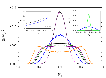
At intermediate densities, the driven system exhibits local ordering into A- and B-rich stripes, without global ordering of the pattern; an example is shown in Fig. 8. To quantify local ordering, we consider a function that essentially projects regions of size $\lambda$ onto a patch of an ideal pattern. Consider a rectangle of $\lambda\times\ell$ sites, i.e., $\mathcal{R}\equiv\{1\leq x\leq\lambda\}\times\{1\leq y\leq\ell\}$. Let $Q_{1}$ be the excess number of A particles over B particles in the left half ($1\leq x\leq\lambda/2$) and $Q_{2}$ the excess number in the right half; define

$$\psi_{\mathcal{R}}=\frac{Q_{1}-Q_{2}}{\lambda\ell}\,.$$ (11)

This quantity takes nonzero values when the region is centered on a stripe of width $\lambda$, but will be close to zero in random configurations, or in regions occupied by a single species. Thus a convenient measure of local ordering is $\Psi=\langle|\psi_{\mathcal{R}}|\rangle-\langle|\psi_{\mathcal{R}}|\rangle_{r}$, where the first average is over configurations in the stationary state at a given density, and the second is over configurations (of the same density) generated by inserting A and B particles, with equal probabilities, at random into $\mathcal{R}$, subject to the prohibition against A-B nearest-neighbor pairs. The probability density $p(\psi)$ changes from unimodal to bimodal at a certain density, marking the growth of local order. In Fig. 12, for $p=1$, the transition from unimodal to bimodal occurs near $\rho=0.65$. This does not imply, of course, that there is no local ordering below this density. The behavior of $\Psi$ is quite smooth over the range of densities of interest (see right inset of Fig. 12), suggesting that there is no phase transition associated with local ordering. For weaker drives, the transition from a unimodal to a bimodal distribution occurs at a similar density: $\rho=0.66$ for $p=1/2$, and $\rho=0.63$ for $p=1/4$. Thus, under a drive, short-range order appears at a density slightly above the equilibrium critical density, $\rho_{c}=0.618(1)$.

Figure 12: (Color online) Probability densities $p(\psi_{\mathcal{R}})$ of the local order (using $\lambda=10$ and $\ell=20$), for densities (upper to lower at center) 0.5, 0.6, 0.64, 0.65, 0.66 and 0.7. Drive parameters $p=1$ and $a=0$, system size $L=100$. Right inset: $p(\psi_{\mathcal{R}})$ for $\rho=0.6$ as in main graph (broad curve), compared with $p_{r}\,(\psi_{\mathcal{R}})$, for randomly generated configurations at the same density (central curve). Right inset: $\langle|\psi_{\mathcal{R}}|\rangle$ (upper dashed curve), $\langle|\psi_{\mathcal{R}}|\rangle_{r}$ (lower dashed curve), and their difference, $\Psi$ (central curve), versus density.

IV.3 Order parameter and phase boundary

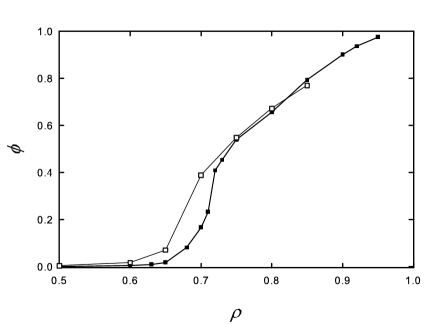
Given the evidence of phase separation discussed above, in the form of A- and B-rich stripes oriented perpendicular to the drive, we turn to a more quantitative discussion, which requires definition of an order parameter. The ordered phase is characterized by charge-density oscillations along the drive, i.e., a correlation function $C_{||}(r)\simeq A\exp[iq^{*}r]$ and an associated structure factor $S_{||,q}$ with a maximum (at $q=q^{*}$) proportional to $(LA)^{2}$. We therefore define the order parameter $\phi=S_{||,q*}/L^{2}$. The order parameter is plotted versus density in Fig. 13 for $p=1$ and $a=0$; the plot strongly suggests that there is a continuous phase transition at a density near 0.72.

Figure 13: Order parameter versus density for $p=1$, $a=0$ and $L=240$ (filled symbols) and 120 (open symbols). Lines are guides to the eye; error bars smaller than symbols.

To obtain a more precise estimate of the density $\rho_{c}$ marking the onset of global order, we perform a finite-size analysis of the order parameter $\phi$. For fixed $p$ and $\rho$ (and $a=0$), we determine $\phi$ for a series of system sizes $L$. In the disordered phase, we expect $\phi$ to decrease rapidly with $L$, whereas in the ordered phase it must approach a nonzero limiting value as $L\to\infty$. A phase transition is marked by slow decay of the order parameter with $L$, typically a power law, $\phi\sim L^{-\beta/\nu_{||}}$. Thus in a plot of $\ln\phi$ versus $\ln L$ for fixed density $\rho$, we interpret upward (downward) curvature as a signal of the ordered (disordered) phase.

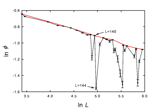
Estimating $\rho_{c}$ is complicated by the fact that as one varies the density, the preferred wavelength changes, as shown in Fig. 11. We obtain more orderly patterns (higher values of $\phi$) using system sizes $L$ that are integer multiples of the preferred wavelength. (Note that the latter need not be an integer. For $p=1$ and $\rho=0.74$, for example, the preferred wavelength is 10.63.) A well ordered pattern consists of an integer number of wavelengths, which is only possible for specific system sizes. This leads to an irregular variation of $\phi$ with $L$, as shown in Fig. 14. Small changes in $L$ (for example, from 140 to 144) can yield large (and reproducible) changes in $\phi$. The various points on the graph of $\phi$ versus $L$ can nevertheless be bounded from above by a smooth “envelope.” The points falling on or near the envelope represent the most ordered cases; we therefore apply the curvature criterion described above to the envelope. For the data shown in Fig. 14, the $\lambda$ values associated with points along the envelope fall in the range 10.50 - 10.77, with a mean of 10.63(5), providing an estimate of the preferred wavelength. We also note that in this case, the envelope is fairly well described by a power law, with an exponent $\beta/\nu_{||}=0.173(5)$.

We adopt the following procedure to determine $\phi$ as a function of $L$:

1. Perform a survey of L values, to estimate the preferred wavelength $\lambda$.

2. Determine $\phi$ for a series of system sizes $L$ such that there is an integer $n$ with $L/n$ falling near $\lambda$.

3. If necessary, refine the estimate for the preferred wavelength and return to 2.

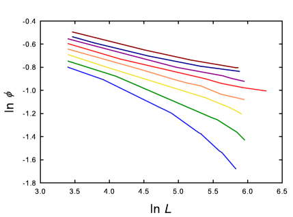
Varying the density from 0.71 to 0.78 (for fixed $p=1$ and $a=0$), we find the set of envelopes shown in Fig. 15. For $\rho\leq 0.73$ the envelopes curve downward, while for $0.74\leq\rho\leq 0.76$ there is no clear curvature; for $\rho\geq 0.77$ the data appear to curve upward. Thus the onset of global order occurs at a density close to 0.77. For densities in the range 0.74-0.76, the order parameter appears to decay as a power law of the system size, with an exponent $\beta/\nu_{||}$ varying between about 0.173 and 0.143. For a small drive ($p=1/8$, $a=0$), a similar analysis shows that the transition occurs at $\rho\simeq 0.73$. Determining the precise value of $\rho_{c}$ as a function of the drive parameters, and verifying the existence of a “critical phase” in which the order parameter scales as an inverse power of $L$, will require extensive studies of larger systems, a task we defer to future work.

Figure 14: Order parameter versus system size for $p=1$, $a=0$ and $\rho=0.74$. Values for system sizes 140 and 144 are highlighted for comparison. The bold line represents the envelope.

Figure 15: (Color online) Envelope of order parameter for $p=1$, $a=0$ and (lower to upper) $\rho=0.71$, 0.72,…, 0.78.

IV.4 Correlation functions

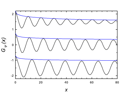
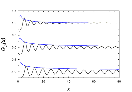
Along with the local and global order parameters discussed above, two-point correlation functions afford insight into the organization of the driven system. The charge-charge and density-density correlation functions are plotted in Figs. 16 and 17, respectively, for maximum drive. $G_{\psi||}$ exhibits the oscillations expected given the stripe pattern. Interestingly, the decay of $G_{\psi\perp}$, which reflects the persistence of stripes in the direction perpendicular to the drive, decays in a manner qualitatively similar to the envelope of the oscillations in $G_{\psi||}$. The density-density correlation function along the drive, $G_{\rho||}$, exhibits weak oscillations at twice the spatial frequency as the charge-charge correlation, reflecting a reduction in density at the interfaces between stripes.

At the lowest density ($\rho=0.7$) shown in the figures, all four correlation functions decay in a manner best described by a stretched exponential, $G\sim\exp[-(x/\xi)^{\beta}]$, with exponents $\beta$ ranging from 0.36 (for $G_{\rho||}$) to 0.55 (for $G_{\psi||}$ and $G_{\psi\perp}$. (For correlations along the drive, the envelope of the oscillations decays as a stretched exponential.) For density 0.75, stretched-exponential decay is again observed, with $\beta\simeq 0.2$, except in the case of $G_{\psi\perp}$, which is better fit by a power law, $G\sim 1/r^{\alpha}$, with $\alpha=0.133$. At density 0.8, $G_{\psi||}$ approaches a nonzero limit of about 0.41 as $x\to\infty$, marking long-range coherence of the stripe pattern. The other correlation functions decay as power laws, with exponents $\alpha=0.080$ (for $G_{\psi\perp}$), 0.62 (for $G_{\rho||}$) and 0.33 ($G_{\rho\perp}$). Thus, correlations decay more slowly at higher density. A nonzero limiting value of $G_{\psi||}$ provides an alternative for detecting long-range order; we defer a systematic analysis using this criterion to future work.

Figure 16: (Color online) Charge-charge correlation functions $G_{\psi||}(x)$, along drive (oscillating), and $G_{\psi\perp}(x)$, perpendicular to drive (decaying monotonically), for $p=1$, $a=0$ and (upper to lower) density $\rho=0.7$, 0.75 and 0.8. The curves for $\rho=0.7$ (0.8) have been shifted upward (downward) by 1.5 for legibility.

Figure 17: (Color online) Density-density correlation functions $G_{\rho||}(x)$, along drive (oscillating), and $G_{\rho\perp}(x)$, perpendicular to drive (decaying monotonically for $x\geq 2$), for parameters as in Fig. 16. The correlation functions are multiplied by 10, and curves for $\rho=0.7$ (0.8) have been shifted upward (downward) by 1, for legibility.

IV.5 Interface width

As shown above, the boundary between A- and B-rich phases defines an interface oriented, on average, perpendicular to the drive, but with significant fluctuations. Thus the scaling properties of the interface width with time and system size are of interest. We examine these properties in the single-stripe regime, in which identification of the interface is relatively simple. Given a configuration, we define for each $j=1,...,L$ in the direction perpendicular to the drive, and for $\ell=1,...,L$ along the drive, the function,

$$s(\ell,j)\equiv\sum_{i=1}^{\ell}\sigma_{i,j}.$$ (12)

Since $s(\ell,j)$ represents the excess of A particles over B particles in the first $\ell$ sites in row $j$, the values of $\ell$ for which $s(\ell,j)$ takes its maximum and minimum correspond to the interface positions in this row. (If the sites at which the maximum or minimum values occur are not unique, we use the smallest $\ell$ at which the extremum occurs.) Given the set of sites $\ell_{+}(j)$ marking the maximum, we construct a random walk representation of the interface, $h_{+}(j)$, by setting $h_{+}(1)=0$ and, for $j\geq 2$, taking $h_{+}(j)=h_{+}(j-1)+[\ell_{+}(j)-\ell_{+}(j-1)]$, where the difference in the square brackets is calculated under periodic boundaries. A second interface is constructed using the positions at which $s(\ell,j)$ takes its minimum. The width of each interface is given by,

$$w=\left\{\frac{1}{L}\sum_{j=1}^{L}\left[h_{+}(j)-\overline{h}\right]^{2}\right\}^{1/2},$$ (13)

where $\overline{h}=(1/L)\sum_{j=1}^{L}h_{+}(j)$.

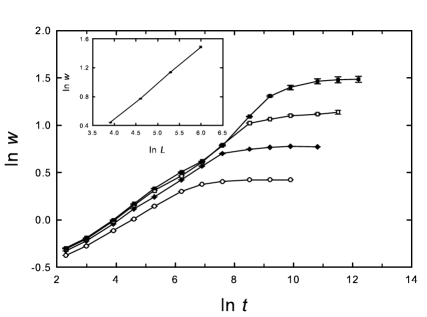
We examine the scaling properties of the interface width as a function of time and system size, plotting, in Fig. 18 (main graph), the width versus time for system sizes $L=50$, 100, 200 and 400, and (inset) the saturation (long-time) width $w_{sat}$ versus system size. These data are for $p=1/3$, $a=0$, and density $\rho=0.85$ (single-stripe regime). The data for $w(t)$ do not follow simple power laws, and cannot be collapsed onto a single curve by rescaling time and width. It is nevertheless possible to estimate the growth exponent $\beta_{w}$ (associated with the behavior $w\sim t^{\beta_{w}}$) using the most linear portions of the graphs (specifically, the second through fifth points in the present case), yielding $\beta_{w}=0.182(3)$, 0.205(4), 0.223(5) and 0.228(6), for system sizes 50 through 400, respectively. The expected scaling of the saturation width, $w_{sat}\sim L^{\alpha}$ is satisfied to reasonable approximation; for $L\geq 100$ we find $\alpha=0.516(6)$. We note that the exponent values are not very different from those of the Edwards-Wilkinson (EW) class, $\alpha=1/2$ and $\beta_{w}=1/4$; it is conceivable that the observed deviations reflect finite-size effects. We defer a more precise determination of the interface width, including analyses of multi-stripe systems, to future work.

Figure 18: Interface width $w$ versus time for $p=1/3$, $a=0$ and system sizes $L=50$, 100, 200 and 400 (lower to upper). Inset: $w_{sat}$ versus $L$.

V Summary and outlook

We study nonequilibrium stationary properties of a Widom-Rowlinson lattice gas subject to a drive favoring particle hopping along one axis and suppressing hopping to the opposite direction. The stationary properties are surprisingly different from those of the driven lattice gas with attractive interactions. As in the equilibrium WRLG wrlg , there is a phase transition with segregation between particle species as the density is increased; the critical density for phase separation increases with drive. We find that even in the disordered phase, there is a preferred wavelength $\lambda$ evident in the charge-charge correlation function along the drive direction, and that the associated structure factor $S(k,0)$ does not take the usual Ornstein-Zernike form. With increasing density, local ordering into A- and B-rich regions occurs, with the appearance of stripes oriented perpendicular to the drive, but without global coherence. Increasing the density further, we observe a transition to a stripe pattern with long-range order. We characterize the system in terms of local and global order parameters, correlation functions and associated structure factors, and provide preliminary results on interface roughness and the particle current provoked by the drive.

Our study leaves many intriguing questions for future study. Among them, we highlight:

1. Why does phase separation result in stripes of a characteristic width, $\lambda$, instead of two regions, as happens in equilibrium? Simulations suggest that very broad stripes are unstable, but the underlying mechanism is unclear.

2. Why do the stripes form perpendicular to the drive? Again, we observe an instability in an interface oriented parallel to the drive - undulations on such an interface tend to grow - but a quantitative explanation is lacking.

3. Can one develop a hydrodynamic description or time-dependent Ginzburg-Landau theory capable of reproducing the phenomenology observed in simulations? Can one derive a quantitative prediction for the current? We find (Sec. III) that although simple mean-field analyses do not predict the phase diagram, they do yield quite good predictions for the current.

4. What is the nature of the phase transition to long-range order of the stripe pattern? Can it be connected to (equilibrium) transitions in smectic liquid crystals?

5. Do the scaling properties of the interfaces fall in the Edwards-Wilkinson class, or some other known class of growth processes?

6. To what extent does entropy maximization, which is the sole factor determining static properties at equilibrium, hold in the driven system, particularly for a weak drive? Related to this, is the zero-drive limit smooth or singular?

Although these and other questions remain open, our study demonstrates that the driven Widom-Rowlinson lattice gas exhibits surprising behaviors not previously observed in driven systems.