Fast eigenpairs computation
with operator adapted wavelets and hierarchical subspace correction

Hehu Xie hhxie@lsec.cc.ac.cn. LSEC, NCMIS, Institute of Computational Mathematics, Academy of Mathematics and Systems Science, Chinese Academy of Sciences, Beijing 100190, China, and University of Chinese Academy of Sciences, Beijing 100049, China.      Lei Zhang111lzhang2012@sjtu.edu.cn. School of Mathematical Sciences, Institute of Natural Sciences, and Ministry of Education Key Laboratory of Scientific and Engineering Computing (MOE-LSC), Shanghai Jiao Tong University, 800 Dongchuan Road, Shanghai 200240, China.      Houman Owhadi222owhadi@caltech.edu. California Institute of Technology, Computing & Mathematical Sciences, MC 9-94 Pasadena, CA 91125.
Abstract

We present a method for the fast computation of the eigenpairs of a bijective positive symmetric linear operator \mathcal{L}. The method is based on a combination of operator adapted wavelets (gamblets) with hierarchical subspace correction. First, gamblets provide a raw but fast approximation of the eigensubspaces of \mathcal{L} by block-diagonalizing \mathcal{L} into sparse and well-conditioned blocks. Next, the hierarchical subspace correction method, computes the eigenpairs associated with the Galerkin restriction of \mathcal{L} to a coarse (low dimensional) gamblet subspace, and then, corrects those eigenpairs by solving a hierarchy of linear problems in the finer gamblet subspaces (from coarse to fine, using multigrid iteration). The proposed algorithm is robust to the presence of multiple (a continuum of) scales and is shown to be of near-linear complexity when \mathcal{L} is an (arbitrary local, e.g. differential) operator mapping 0s(Ω)subscriptsuperscript𝑠0Ω\mathcal{H}^{s}_{0}(\Omega) to s(Ω)superscript𝑠Ω\mathcal{H}^{-s}(\Omega) (e.g. an elliptic PDE with rough coefficients).

Keywords. Multiscale eigenvalue problem, gamblet decomposition, multigrid iteration, subspace correction, numerical homogenization.

AMS subject classifications. 65N30, 65N25, 65L15, 65B99.

1 Introduction

Solving large scale eigenvalue problems is one of the most fundamental and challenging tasks in modern science and engineering. Although high-dimensional eigenvalue problems are ubiquitous in physical sciences, data and imaging sciences, and machine learning, the class of eigensolvers is not as diverse as that of linear solvers (which comprises many efficient algorithms such as geometric and algebraic multigrid [11, 20], approximate Gaussian elimination [33], etc.). In particular, eigenvalue problems may involve operators with nonseparable multiple scales, and the nonlinear interplay between those coupled scales and the eigenvalue problem poses significant challenges for numerical analysis and scientific computing [4, 14, 59, 37].

Krylov subspace type methods remain the most reliable and efficient tools for large scale eigenproblems, and alternative approaches such as optimization based methods and nonlinear solver based methods have been pursued in the recent years. For example, the Implicitly Restarted Lanczos/Arnoldi Method (IRLM/IRAM) [49], the Preconditioned INVerse ITeration (PINVIT) method [19, 10, 24], the Locally Optimal Block Preconditioned Conjugate Gradient (LOBPCG) method [25, 28], and the Jacobi-Davidson-type techniques [7] have been developed. For those state-of-the-art eigensolvers, the efficient application of preconditioning [24] is often crucial for the faster convergence and the reduction of computation cost, especially for multiscale eigenproblems.

Recently, two-level [57, 37] and multilevel [34, 35, 36, 55, 56] correction methods have been proposed to reduce the complexity of solving eigenpairs associated with low eigenvalues by first solving a coarse mesh/scale approximation, which can then be corrected by solving linear systems (corresponding to linearized eigenvalue problems) on a hierarchy of finer meshes/scales. Although the multilevel correction approach has been extended to multigrid methods for linear and nonlinear eigenvalue problems [16, 34, 35, 36, 23, 55, 56], the regularity estimates required for linear complexity do not hold for PDEs with rough coefficients and a naive application of the correction approach to multiscale eigenvalue problems may converge very slowly. For two-level methods [57] this lack of robustness can be alleviated by numerical homogenization techniques [37], e.g., the so-called Localized Orthogonal Decomposition (LOD) method. For multilevel methods, gamblets [41, 42, 44, 48, 43] (operator-adapted wavelets satisfying three desirable properties: scale orthogonality, well-conditioned multi-resolution decomposition, and localization) provide a natural multiresolution decomposition ensuring robustness for multiscale eigenproblems. As described in [43, Sec. 5.1.3], these three properties are analogous to those required of Wannier functions [29, 54], which can be characterized as linear combinations χi=jci,jvjsubscript𝜒𝑖subscript𝑗subscript𝑐𝑖𝑗subscript𝑣𝑗\chi_{i}=\sum_{j}c_{i,j}v_{j} of eigenfunctions vjsubscript𝑣𝑗v_{j} associated with eigenvalues λjsubscript𝜆𝑗\lambda_{j} such that the size of ci,jsubscript𝑐𝑖𝑗c_{i,j} is large for λjsubscript𝜆𝑗\lambda_{j} close to λisubscript𝜆𝑖\lambda_{i} and small otherwise, and such that the resulting linear combinations χisubscript𝜒𝑖\chi_{i} are concentrated in space.

The aim of this paper is therefore to design a fast multilevel numerical method for multiscale eigenvalue problems (e.g. for PDEs that may have rough and highly oscillatory coefficients) associated with a bijective positive symmetric linear operator \mathcal{L}, by integrating the multilevel correction approach with the gamblet multiresolution decomposition. In this merger, the gamblet decomposition supplies a hierarchy of coarse (sub)spaces for the multilevel correction method. The overall computational cost is that of solving a sequence of linear problems over this hierarchy (using a gamblet based multigrid approach [41]). Recently, Hou et. al. [21] proposed to compute the leftmost eigenpairs of a sparse symmetric positive matrix by combining the implicitly restarted Lanczos method with a gamblet-like multiresolution decomposition where local eigenfunctions are used as measurement functions. This paper shows that the gamblet multilevel decomposition (1) enhances the convergence rate of eigenvalue solvers by enabling (through a gamblet based multigrid method) the fast and robust convergence of inner iterations (linear solves) in the multilevel correction method, and (2) provides efficient preconditioners for state-of-the-art eigensolvers such as the LOBPCG method.

Outline

This paper is organized as follows: We summarize the gamblet decomposition, its properties, and the gamblet based multigrid method in Section § 2 (see [41, 42, 44, 48, 43] for the detailed construction). We present the gamblet based multilevel method for multiscale eigenvalue problems and its rigorous analysis in Section § 3. Our theoretical results are numerically illustrated in Section § 4 where the proposed method is compared with state-of-the-art eigensolvers (such as LOBPCG).

Notation

The symbol C𝐶C denotes generic positive constant that may change from one line of an estimate to the next. C𝐶C will be independent from the eigenvalues (otherwise a subscript λ𝜆\lambda will be added), and the dependencies of C𝐶C will normally be clear from the context or stated explicitly.

2 Gamblet Decomposition and Gamblet based Multigrid Method

Although multigrid methods [11, 20] have been highly successful in solving elliptic PDEs, their convergence rates can be severely affected by the lack of regularity of the PDE coefficients [53]. Although classical wavelet based methods [13, 17] enable a multi-resolution decomposition of the solution space, their performance can also be affected by their lack of adaptation to the coefficients of the PDE. The introduction of gamblets in [41] addressed the problem of designing multigrid/multiresolution methods that are provably robust with respect to rough (Lsuperscript𝐿L^{\infty}) PDE coefficients.

Gamblets are derived from a game theoretic approach to numerical analysis [41, 42]. They (1) are elementary solutions of hierarchical information games associated with the process of computing with partial information and limited resources, (2) have a natural Bayesian interpretation under the mixed strategy emerging from the game theoretic formulation, (3) induce a multi-resolution decomposition of the solution space that is adapted to the numerical discretization of the underlying PDE. The (fast) gamblet transform has 𝒪(Nlog2d+1N)𝒪𝑁superscript2𝑑1𝑁\mathcal{O}(N\log^{2d+1}N) complexity for the first solve and 𝒪(Nlogd+1N)𝒪𝑁superscript𝑑1𝑁\mathcal{O}(N\log^{d+1}N) for subsequent solves to achieve grid-size accuracy in H1superscript𝐻1H^{1}-norm for elliptic problems [43].

2.1 The abstract setting

We introduce the formulation of gamblets with an abstract setting since its application is not limited to scalar elliptic problems such as examples 2.1 and 2.2. Let (V,),(V,)(V,\|\cdot\|),(V^{*},\|\cdot\|_{*}) and (V0,0)(V_{0},\|\cdot\|_{0}) be Hilbert spaces such that VV0V𝑉subscript𝑉0superscript𝑉V\subset V_{0}\subset V^{*} and such that the natural embedding i:V0V:𝑖subscript𝑉0superscript𝑉i:V_{0}\rightarrow V^{*} is compact and dense. Let (V,)(V^{*},\|\cdot\|_{*}) be the dual of (V,)(V,\|\cdot\|) using the dual pairing obtained from the Gelfand triple.

Let the operator \mathcal{L} be a symmetric positive linear bijection mapping V𝑉V to Vsuperscript𝑉V^{*}. Write [,][\cdot,\cdot] for the duality pairing between Vsuperscript𝑉V^{*} and V𝑉V (derived from the Riesz duality between V0subscript𝑉0V_{0} and itself) such that

u2=[u,u] for uV.superscriptnorm𝑢2𝑢𝑢 for 𝑢𝑉\|u\|^{2}=[\mathcal{L}u,u]\text{ for }u\in V\,. (2.1)

The corresponding inner product on V𝑉V is defined by

u,v:=[u,v]for u,vV,formulae-sequenceassign𝑢𝑣𝑢𝑣for 𝑢𝑣𝑉\big{\langle}u,v\big{\rangle}:=[\mathcal{L}u,v]\quad\text{for }u,v\in V, (2.2)

and \|\cdot\|_{*} is the corresponding dual-norm on Vsuperscript𝑉V^{*}, i.e.

ϕ=supvV,v0[ϕ,v]v for ϕV.subscriptnormitalic-ϕsubscriptsupremumformulae-sequence𝑣𝑉𝑣0italic-ϕ𝑣norm𝑣 for italic-ϕsuperscript𝑉\|\phi\|_{*}=\sup_{v\in V,v\neq 0}\frac{[\phi,v]}{\|v\|}\text{ for }\phi\in V^{*}\,. (2.3)

Given gV𝑔superscript𝑉g\in V^{*}, we will consider the solution u𝑢u of the variational problem

u,v=[g,v], for vV.formulae-sequence𝑢𝑣𝑔𝑣 for 𝑣𝑉\big{\langle}u,v\big{\rangle}=[g,v],\quad\text{ for }v\in V\,. (2.4)
Example 2.1.

Let ΩΩ\Omega be a bounded open subset of dsuperscript𝑑\mathbb{R}^{d} (of arbitrary dimension d𝑑superscriptd\in\mathbb{N}^{*}) with uniformly Lipschitz boundary. Given s𝑠s\in\mathbb{N}, let

:0s(Ω)s(Ω):subscriptsuperscript𝑠0Ωsuperscript𝑠Ω\mathcal{L}\,:\,\mathcal{H}^{s}_{0}(\Omega)\rightarrow\mathcal{H}^{-s}(\Omega) (2.5)

be a continuous linear bijection between 0s(Ω)subscriptsuperscript𝑠0Ω\mathcal{H}^{s}_{0}(\Omega) and s(Ω)superscript𝑠Ω\mathcal{H}^{-s}(\Omega), where 0s(Ω)subscriptsuperscript𝑠0Ω\mathcal{H}^{s}_{0}(\Omega) is the Sobolev space of order s𝑠s with zero trace, and s(Ω)superscript𝑠Ω\mathcal{H}^{-s}(\Omega) is the topological dual of 0s(Ω)subscriptsuperscript𝑠0Ω\mathcal{H}^{s}_{0}(\Omega) [1]. Assume \mathcal{L} to be symmetric, positive and local, i.e. [u,v]=[u,v]𝑢𝑣𝑢𝑣[\mathcal{L}u,v]=[u,\mathcal{L}v] and [u,u]0𝑢𝑢0[\mathcal{L}u,u]\geq 0 for u,v0s(Ω)𝑢𝑣subscriptsuperscript𝑠0Ωu,v\in\mathcal{H}^{s}_{0}(\Omega) and [u,v]=0𝑢𝑣0[\mathcal{L}u,v]=0 if u,v𝑢𝑣u,v have disjoint supports in ΩΩ\Omega. In this example V,V𝑉superscript𝑉V,V^{*} and V0subscript𝑉0V_{0} are 0s(Ω)subscriptsuperscript𝑠0Ω\mathcal{H}^{s}_{0}(\Omega), s(Ω)superscript𝑠Ω\mathcal{H}^{-s}(\Omega) and L2(Ω)superscript𝐿2ΩL^{2}(\Omega) endowed with the norms u2=Ωuusuperscriptnorm𝑢2subscriptΩ𝑢𝑢\|u\|^{2}=\int_{\Omega}u\mathcal{L}u, ϕ2=Ωϕ1ϕsuperscriptsubscriptnormitalic-ϕ2subscriptΩitalic-ϕsuperscript1italic-ϕ\|\phi\|_{*}^{2}=\int_{\Omega}\phi\mathcal{L}^{-1}\phi and u0=uL2(Ω)subscriptnorm𝑢0subscriptnorm𝑢superscript𝐿2Ω\|u\|_{0}=\|u\|_{L^{2}(\Omega)}.

Example 2.2.

Consider Example 2.1 with s=1𝑠1s=1, =div(a(x))\mathcal{L}=-\operatorname{div}\big{(}a(x)\nabla\cdot\big{)} and a(x)𝑎𝑥a(x) is a symmetric, uniformly elliptic d×d𝑑𝑑d\times d matrix with entries in L(Ω)superscript𝐿ΩL^{\infty}(\Omega) such that for all xΩ𝑥Ωx\in\Omega and dsuperscript𝑑\ell\in\mathbb{R}^{d},

λmin(a)||2Ta(x)λmax(a)||2.subscript𝜆𝑎superscript2superscript𝑇𝑎𝑥subscript𝜆𝑎superscript2\lambda_{\min}(a)|\ell|^{2}\leq\ell^{T}a(x)\ell\leq\lambda_{\max}(a)|\ell|^{2}. (2.6)

Note that

v2=Ω(v)Tav for v01(Ω),formulae-sequencesuperscriptnorm𝑣2subscriptΩsuperscript𝑣𝑇𝑎𝑣 for 𝑣subscriptsuperscript10Ω\|v\|^{2}=\int_{\Omega}(\nabla v)^{T}a\nabla v\ \ \text{ for }v\in\mathcal{H}^{1}_{0}(\Omega)\,, (2.7)

and the solution of (2.4) is the solution of the PDE

{div(a(x)u(x))=g(x)xΩ,u=0onΩ.casesformulae-sequencediv𝑎𝑥𝑢𝑥𝑔𝑥𝑥Ωotherwise𝑢0onΩotherwise\begin{cases}-\operatorname{div}\big{(}a(x)\nabla u(x)\big{)}=g(x)\quad x\in\Omega,\\ u=0\quad\text{on}\quad\partial\Omega\,.\end{cases} (2.8)

2.2 Gamblets

Here we give a brief reminder of the construction of gamblets. See Example 2.3 for a concrete example for scalar elliptic equation and Section § 4.1 for the numerical implementation, and also [41, 42, 44, 48, 43] for more details.

Measurement functions.

Let (1),,(q)superscript1superscript𝑞\mathcal{I}^{(1)},\ldots,\mathcal{I}^{(q)} be a hierarchy of labels and let ϕi(k)superscriptsubscriptitalic-ϕ𝑖𝑘\phi_{i}^{(k)} be a hierarchy of nested elements of Vsuperscript𝑉V^{*} such that

ϕi(k)=j(k+1)πi,j(k,k+1)ϕj(k+1) for k{1,,q1} and i(k),formulae-sequencesuperscriptsubscriptitalic-ϕ𝑖𝑘subscript𝑗superscript𝑘1subscriptsuperscript𝜋𝑘𝑘1𝑖𝑗superscriptsubscriptitalic-ϕ𝑗𝑘1 for 𝑘1𝑞1 and 𝑖superscript𝑘\phi_{i}^{(k)}=\sum_{j\in\mathcal{I}^{(k+1)}}\pi^{(k,k+1)}_{i,j}\phi_{j}^{(k+1)}\ \ \text{ for }k\in\{1,\ldots,q-1\}\text{ and }i\in\mathcal{I}^{(k)}\,, (2.9)

for some rank |(k)|superscript𝑘|\mathcal{I}^{(k)}|, (k)×(k+1)superscript𝑘superscript𝑘1\mathcal{I}^{(k)}\times\mathcal{I}^{(k+1)} matrices π(k,k+1)superscript𝜋𝑘𝑘1\pi^{(k,k+1)} and such that the (ϕi(k))i(k)subscriptsuperscriptsubscriptitalic-ϕ𝑖𝑘𝑖superscript𝑘(\phi_{i}^{(k)})_{i\in\mathcal{I}^{(k)}} are linearly independent and π(k,k+1)π(k+1,k)=I(k)superscript𝜋𝑘𝑘1superscript𝜋𝑘1𝑘subscript𝐼superscript𝑘\pi^{(k,k+1)}\pi^{(k+1,k)}=I_{\mathcal{I}^{(k)}} for k{1,,q1}𝑘1𝑞1k\in\{1,\ldots,q-1\} (writing I𝒥subscript𝐼𝒥I_{\mathcal{J}} for the 𝒥×𝒥𝒥𝒥\mathcal{J}\times\mathcal{J} identity matrix and π(k+1,k)superscript𝜋𝑘1𝑘\pi^{(k+1,k)} for (π(k,k+1))Tsuperscriptsuperscript𝜋𝑘𝑘1𝑇(\pi^{(k,k+1)})^{T}). Although not required in the general theory of gamblets [43] in this paper we assume that the ϕi(k)superscriptsubscriptitalic-ϕ𝑖𝑘\phi_{i}^{(k)} are elements of V0subscript𝑉0V_{0} and have uniformly well conditioned mass matrices in the sense that C1|x|2ixiϕi(k)02C|x|2superscript𝐶1superscript𝑥2superscriptsubscriptnormsubscript𝑖subscript𝑥𝑖superscriptsubscriptitalic-ϕ𝑖𝑘02𝐶superscript𝑥2C^{-1}|x|^{2}\leq\|\sum_{i}x_{i}\phi_{i}^{(k)}\|_{0}^{2}\leq C|x|^{2} (for all x𝑥x and k𝑘k).

Operator adapted pre-wavelets.

For k{1,,q}𝑘1𝑞k\in\{1,\ldots,q\}, let Θ(k)superscriptΘ𝑘\Theta^{(k)} be the symmetric positive definite matrix with entries Θi,j(k):=[ϕi(k),1ϕj(k)]assignsubscriptsuperscriptΘ𝑘𝑖𝑗superscriptsubscriptitalic-ϕ𝑖𝑘superscript1superscriptsubscriptitalic-ϕ𝑗𝑘\Theta^{(k)}_{i,j}:=[\phi_{i}^{(k)},\mathcal{L}^{-1}\phi_{j}^{(k)}] and (writing Θ(k),1superscriptΘ𝑘1\Theta^{(k),-1} for the inverse of Θ(k)superscriptΘ𝑘\Theta^{(k)}) let

ψi(k)=j(k)Θi,j(k),1ϕj(k) for i(k).formulae-sequencesuperscriptsubscript𝜓𝑖𝑘subscript𝑗superscript𝑘subscriptsuperscriptΘ𝑘1𝑖𝑗superscriptsubscriptitalic-ϕ𝑗𝑘 for 𝑖superscript𝑘\psi_{i}^{(k)}=\sum_{j\in\mathcal{I}^{(k)}}\Theta^{(k),-1}_{i,j}\phi_{j}^{(k)}\ \ \text{ for }i\in\mathcal{I}^{(k)}\,. (2.10)

The elements ψi(k)superscriptsubscript𝜓𝑖𝑘\psi_{i}^{(k)} form a bi-orthogonal system with respect to the elements ϕi(k)superscriptsubscriptitalic-ϕ𝑖𝑘\phi_{i}^{(k)}, i.e. [ϕj(k),ψi(k)]=δi,jsuperscriptsubscriptitalic-ϕ𝑗𝑘superscriptsubscript𝜓𝑖𝑘subscript𝛿𝑖𝑗[\phi_{j}^{(k)},\psi_{i}^{(k)}]=\delta_{i,j} and

u(k):=i(k)[ϕi(k),u]ψi(k),assignsuperscript𝑢𝑘subscript𝑖superscript𝑘superscriptsubscriptitalic-ϕ𝑖𝑘𝑢superscriptsubscript𝜓𝑖𝑘u^{(k)}:=\sum_{i\in\mathcal{I}^{(k)}}[\phi_{i}^{(k)},u]\psi_{i}^{(k)}\,, (2.11)

is the ,\big{\langle}\cdot,\cdot\big{\rangle} orthogonal projection of uV𝑢𝑉u\in V onto

𝔙(k):=span{ψi(k)i(k)}.assignsuperscript𝔙𝑘spanconditionalsuperscriptsubscript𝜓𝑖𝑘𝑖superscript𝑘\mathfrak{V}^{(k)}:=\operatorname{span}\{\psi_{i}^{(k)}\mid i\in\mathcal{I}^{(k)}\}\,. (2.12)

Furthermore A(k):=Θ(k),1assignsuperscript𝐴𝑘superscriptΘ𝑘1A^{(k)}:=\Theta^{(k),-1} can be identified as the stiffness matrix of the ψi(k)superscriptsubscript𝜓𝑖𝑘\psi_{i}^{(k)}, i.e.

Ai,j(k)=ψi(k),ψj(k) for i,j(k).formulae-sequencesubscriptsuperscript𝐴𝑘𝑖𝑗superscriptsubscript𝜓𝑖𝑘superscriptsubscript𝜓𝑗𝑘 for 𝑖𝑗superscript𝑘A^{(k)}_{i,j}=\big{\langle}\psi_{i}^{(k)},\psi_{j}^{(k)}\big{\rangle}\ \ \text{ for }i,j\in\mathcal{I}^{(k)}\,. (2.13)

The ψi(k)superscriptsubscript𝜓𝑖𝑘\psi_{i}^{(k)} are nested pre-wavelets in the sense that 𝔙(k)𝔙(k+1)superscript𝔙𝑘superscript𝔙𝑘1\mathfrak{V}^{(k)}\subset\mathfrak{V}^{(k+1)} and

ψi(k)=j(k+1)Ri,j(k,k+1)ψj(k+1),superscriptsubscript𝜓𝑖𝑘subscript𝑗superscript𝑘1subscriptsuperscript𝑅𝑘𝑘1𝑖𝑗superscriptsubscript𝜓𝑗𝑘1\psi_{i}^{(k)}=\sum_{j\in\mathcal{I}^{(k+1)}}R^{(k,k+1)}_{i,j}\psi_{j}^{(k+1)}\,, (2.14)

where R(k,k+1)=A(k)π(k,k+1)Θ(k+1)superscript𝑅𝑘𝑘1superscript𝐴𝑘superscript𝜋𝑘𝑘1superscriptΘ𝑘1R^{(k,k+1)}=A^{(k)}\pi^{(k,k+1)}\Theta^{(k+1)} acts as an interpolation matrix.

Gamblets (operator adapted wavelets).

Let (𝒥(k))2kqsubscriptsuperscript𝒥𝑘2𝑘𝑞(\mathcal{J}^{(k)})_{2\leq k\leq q} be a hierarchy of labels such that (writing |𝒥(k)|superscript𝒥𝑘|\mathcal{J}^{(k)}| for the cardinal of 𝒥(k)superscript𝒥𝑘\mathcal{J}^{(k)}) |𝒥(k)|=|(k)||(k1)|superscript𝒥𝑘superscript𝑘superscript𝑘1|\mathcal{J}^{(k)}|=|\mathcal{I}^{(k)}|-|\mathcal{I}^{(k-1)}|. For k{2,,q}𝑘2𝑞k\in\{2,\ldots,q\}, let W(k)superscript𝑊𝑘W^{(k)} be a 𝒥(k)×(k)superscript𝒥𝑘superscript𝑘\mathcal{J}^{(k)}\times\mathcal{I}^{(k)} matrix such that (writing W(k),Tsuperscript𝑊𝑘𝑇W^{(k),T} for the transpose of W(k)superscript𝑊𝑘W^{(k)})

Ker(π(k1,k))=Im(W(k),T) and W(k)W(k),T=I𝒥(k).Kersuperscript𝜋𝑘1𝑘Imsuperscript𝑊𝑘𝑇 and superscript𝑊𝑘superscript𝑊𝑘𝑇subscript𝐼superscript𝒥𝑘\operatorname{Ker}(\pi^{(k-1,k)})=\operatorname{Im}(W^{(k),T})\text{ and }W^{(k)}W^{(k),T}=I_{\mathcal{J}^{(k)}}\,. (2.15)

Define

χi(k):=j(k)Wi,j(k)ψj(k) k{2,,q} and i𝒥(k) .assignsuperscriptsubscript𝜒𝑖𝑘subscript𝑗superscript𝑘subscriptsuperscript𝑊𝑘𝑖𝑗superscriptsubscript𝜓𝑗𝑘 k{2,,q} and i𝒥(k) \chi_{i}^{(k)}:=\sum_{j\in\mathcal{I}^{(k)}}W^{(k)}_{i,j}\psi_{j}^{(k)}\ \ \text{ $k\in\{2,\ldots,q\}$ and $i\in\mathcal{J}^{(k)}$ }\,. (2.16)

Then u(k)u(k1)superscript𝑢𝑘superscript𝑢𝑘1u^{(k)}-u^{(k-1)} is the ,\big{\langle}\cdot,\cdot\big{\rangle} orthogonal projection of uV𝑢𝑉u\in V onto

𝔚(k):=span{χi(k)i𝒥(k)}.assignsuperscript𝔚𝑘spanconditionalsuperscriptsubscript𝜒𝑖𝑘𝑖superscript𝒥𝑘\mathfrak{W}^{(k)}:=\operatorname{span}\{\chi_{i}^{(k)}\mid i\in\mathcal{J}^{(k)}\}\,. (2.17)

We will also write 𝒥(1):=(1)assignsuperscript𝒥1superscript1\mathcal{J}^{(1)}:=\mathcal{I}^{(1)}, χi(1):=ψi(1)assignsubscriptsuperscript𝜒1𝑖superscriptsubscript𝜓𝑖1\chi^{(1)}_{i}:=\psi_{i}^{(1)}, 𝔚(1):=𝔙(1)assignsuperscript𝔚1superscript𝔙1\mathfrak{W}^{(1)}:=\mathfrak{V}^{(1)}. We call those operator adapted wavelets χi(k)superscriptsubscript𝜒𝑖𝑘\chi_{i}^{(k)}, gamblets. Furthermore 𝔚(k)superscript𝔚𝑘\mathfrak{W}^{(k)} is the ,\big{\langle}\cdot,\cdot\big{\rangle}-orthogonal complement of 𝔙(k1)superscript𝔙𝑘1\mathfrak{V}^{(k-1)} in 𝔙(k)superscript𝔙𝑘\mathfrak{V}^{(k)}, i.e. 𝔙(k)=𝔙(k1)𝔚(k),superscript𝔙𝑘direct-sumsuperscript𝔙𝑘1superscript𝔚𝑘\mathfrak{V}^{(k)}=\mathfrak{V}^{(k-1)}\oplus\mathfrak{W}^{(k)}\,,

𝔙(q)=𝔙(1)𝔚(2)𝔚(q),superscript𝔙𝑞direct-sumsuperscript𝔙1superscript𝔚2superscript𝔚𝑞\mathfrak{V}^{(q)}=\mathfrak{V}^{(1)}\oplus\mathfrak{W}^{(2)}\oplus\cdots\oplus\mathfrak{W}^{(q)}\,, (2.18)

and writing 𝔚(q+1)superscript𝔚𝑞1\mathfrak{W}^{(q+1)} for the ,\big{\langle}\cdot,\cdot\big{\rangle}-orthogonal complement of 𝔙(q)superscript𝔙𝑞\mathfrak{V}^{(q)} in V𝑉V, u=u(1)+(u(2)u(1))++(u(q+1)u(q))𝑢superscript𝑢1superscript𝑢2superscript𝑢1superscript𝑢𝑞1superscript𝑢𝑞u=u^{(1)}+(u^{(2)}-u^{(1)})+\cdots+(u^{(q+1)}-u^{(q)}) is the multiresolution decomposition of u𝑢u over V=𝔙(1)+𝔚(2)++𝔚(q+1)𝑉superscript𝔙1superscript𝔚2superscript𝔚𝑞1V=\mathfrak{V}^{(1)}+\mathfrak{W}^{(2)}+\cdots+\mathfrak{W}^{(q+1)}, namely, the gamblet decomposition of u𝑢u.

For k{2,,q}𝑘2𝑞k\in\{2,\ldots,q\}, B(k)=W(k)A(k)W(k),Tsuperscript𝐵𝑘superscript𝑊𝑘superscript𝐴𝑘superscript𝑊𝑘𝑇B^{(k)}=W^{(k)}A^{(k)}W^{(k),T} is the stiffness matrix of the χi(k)subscriptsuperscript𝜒𝑘𝑖\chi^{(k)}_{i}, i.e.

Bi,j(k)=χi(k),χj(k) for i,j𝒥(k).formulae-sequencesubscriptsuperscript𝐵𝑘𝑖𝑗superscriptsubscript𝜒𝑖𝑘superscriptsubscript𝜒𝑗𝑘 for 𝑖𝑗superscript𝒥𝑘B^{(k)}_{i,j}=\big{\langle}\chi_{i}^{(k)},\chi_{j}^{(k)}\big{\rangle}\ \ \text{ for }i,j\in\mathcal{J}^{(k)}\,. (2.19)

and B(1):=A(1)assignsuperscript𝐵1superscript𝐴1B^{(1)}:=A^{(1)}.

Quantitative estimates.

Under general stability conditions on the ϕi(k)superscriptsubscriptitalic-ϕ𝑖𝑘\phi_{i}^{(k)} [41, 44, 42, 48, 43] these operator adapted wavelets satisfy the quantitative estimates of Property 2.1, we will first state those estimates and provide an example of their validity in the general setting of Example 2.1.

Property 2.1.

The following properties are satisfied for some constant C>0𝐶0C>0 and H(0,1)𝐻01H\in(0,1):

  1. 1

    Approximation:

    uu(k)0CHkuu(k) for uV,subscriptnorm𝑢superscript𝑢𝑘0𝐶superscript𝐻𝑘norm𝑢superscript𝑢𝑘 for 𝑢𝑉\|u-u^{{(k)}}\|_{0}\leq CH^{k}\|u-u^{{(k)}}\|\text{ for }u\in V, (2.20)

    and

    uu(k)CHku0 for u1V0.norm𝑢superscript𝑢𝑘𝐶superscript𝐻𝑘subscriptnorm𝑢0 for 𝑢superscript1subscript𝑉0\|u-u^{{(k)}}\|\leq CH^{k}\|\mathcal{L}u\|_{0}\text{ for }u\in\mathcal{L}^{-1}V_{0}\,. (2.21)
  2. 2

    Uniform bounded condition number: Writing Cond(B)Cond𝐵\operatorname{Cond}(B) for the condition number of a matrix B𝐵B we have for k{1,,q}𝑘1𝑞k\in\{1,\cdots,q\},

    C1H2(k1)I𝒥(k)B(k)CH2kI𝒥(k) and Cond(B(k))CH2.superscript𝐶1superscript𝐻2𝑘1subscript𝐼superscript𝒥𝑘superscript𝐵𝑘𝐶superscript𝐻2𝑘subscript𝐼superscript𝒥𝑘 and Condsuperscript𝐵𝑘𝐶superscript𝐻2C^{-1}H^{-2(k-1)}I_{\mathcal{J}^{{(k)}}}\leq B^{(k)}\leq CH^{-2k}I_{\mathcal{J}^{{(k)}}}\text{ and }\operatorname{Cond}(B^{(k)})\leq CH^{-2}\,. (2.22)

    and

    C1I(k)A(k)CH2kI(k).superscript𝐶1subscript𝐼superscript𝑘superscript𝐴𝑘𝐶superscript𝐻2𝑘subscript𝐼superscript𝑘C^{-1}I_{\mathcal{I}^{{(k)}}}\leq A^{(k)}\leq CH^{-2k}I_{\mathcal{I}^{{(k)}}}\,. (2.23)
  3. 3

    Near linear complexity: The wavelets ψi(k),χi(k)superscriptsubscript𝜓𝑖𝑘superscriptsubscript𝜒𝑖𝑘\psi_{i}^{(k)},\chi_{i}^{(k)} and stiffness matrices A(k),B(k)superscript𝐴𝑘superscript𝐵𝑘A^{(k)},B^{(k)} can be computed to precision ε𝜀\varepsilon (in \|\cdot\|-energy norm for elements of V𝑉V and in Frobenius norm for matrices) in O(NpolylogNε)O𝑁polylog𝑁𝜀\operatorname{O}(N\operatorname{polylog}\frac{N}{\varepsilon}) complexity.

Refer to caption
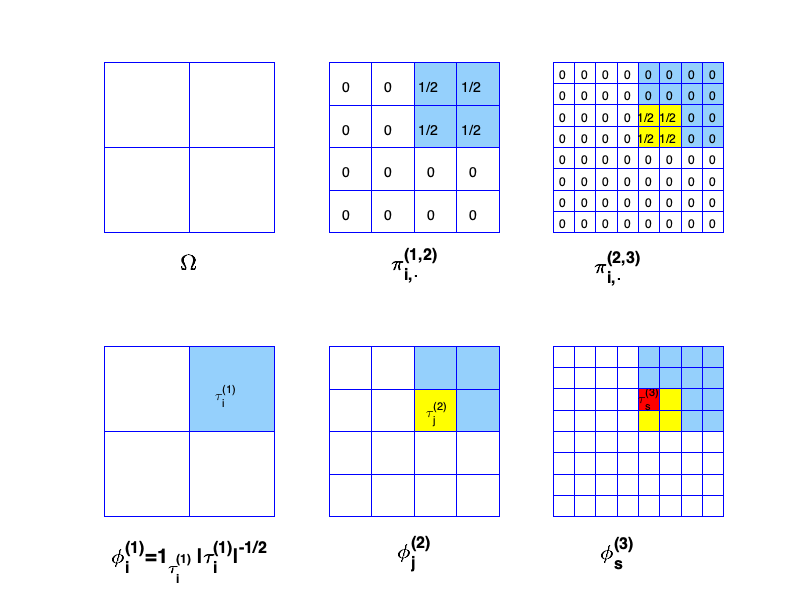
Figure 1: Nested partition of Ω=(0,1)2Ωsuperscript012\Omega=(0,1)^{2} such that the k𝑘kth level corresponds to a uniform partition of ΩΩ\Omega into 2k×2ksuperscript2𝑘superscript2𝑘2^{-k}\times 2^{-k} squares. The top row shows the entries of πi,(1,2)subscriptsuperscript𝜋12𝑖\pi^{(1,2)}_{i,\cdot} and πj,(2,3)subscriptsuperscript𝜋23𝑗\pi^{(2,3)}_{j,\cdot}. The bottom row shows the support of ϕi(1),ϕj(2)superscriptsubscriptitalic-ϕ𝑖1superscriptsubscriptitalic-ϕ𝑗2\phi_{i}^{(1)},\phi_{j}^{(2)} and ϕs(3)superscriptsubscriptitalic-ϕ𝑠3\phi_{s}^{(3)}. Note that j(1)=s(1)=isuperscript𝑗1superscript𝑠1𝑖j^{(1)}=s^{(1)}=i and s(2)=jsuperscript𝑠2𝑗s^{(2)}=j.
Example 2.3.

Consider Example 2.1. Let (q)superscript𝑞\mathcal{I}^{(q)} be the finite set of q𝑞q-tuples of the form i=(i1,,iq)𝑖subscript𝑖1subscript𝑖𝑞i=(i_{1},\ldots,i_{q}). For 1k<q1𝑘𝑞1\leq k<q and a r𝑟r-tuple of the form i=(i1,,iq)𝑖subscript𝑖1subscript𝑖𝑞i=(i_{1},\ldots,i_{q}), write i(k):=(i1,,ik)assignsuperscript𝑖𝑘subscript𝑖1subscript𝑖𝑘i^{(k)}:=(i_{1},\ldots,i_{k}). For 1kq1𝑘𝑞1\leq k\leq q and i=(i1,,iq)(q)𝑖subscript𝑖1subscript𝑖𝑞superscript𝑞i=(i_{1},\ldots,i_{q})\in\mathcal{I}^{(q)}, write (k):={i(k):i(q)}assignsuperscript𝑘conditional-setsuperscript𝑖𝑘𝑖superscript𝑞\mathcal{I}^{(k)}:=\{i^{(k)}\,:\,i\in\mathcal{I}^{(q)}\}. Let δ,h(0,1)𝛿01\delta,h\in(0,1). Let (τi(k))i(k)subscriptsuperscriptsubscript𝜏𝑖𝑘𝑖superscript𝑘(\tau_{i}^{(k)})_{i\in\mathcal{I}^{(k)}} be uniformly Lipschitz convex sets forming a nested partition of ΩΩ\Omega, i.e. such that Ω=i(k)τi(k),k{1,,q}formulae-sequenceΩsubscript𝑖superscript𝑘superscriptsubscript𝜏𝑖𝑘𝑘1𝑞\Omega=\cup_{i\in\mathcal{I}^{(k)}}\tau_{i}^{(k)},\quad k\in\{1,\ldots,q\} is a disjoint union except for the boundaries, and τi(k)=j(k+1):j(k)=iτj(k+1),k{1,,q1}formulae-sequencesuperscriptsubscript𝜏𝑖𝑘subscript:𝑗superscript𝑘1superscript𝑗𝑘𝑖superscriptsubscript𝜏𝑗𝑘1𝑘1𝑞1\tau_{i}^{(k)}=\cup_{j\in\mathcal{I}^{(k+1)}:j^{(k)}=i}\tau_{j}^{(k+1)},\quad k\in\{1,\ldots,q-1\}. Assume that each τi(k)superscriptsubscript𝜏𝑖𝑘\tau_{i}^{(k)}, contains a ball of center xi(k)superscriptsubscript𝑥𝑖𝑘x_{i}^{(k)} and radius δhk𝛿superscript𝑘\delta h^{k}, and is contained in the ball of center xi(k)superscriptsubscript𝑥𝑖𝑘x_{i}^{(k)} and radius δ1hksuperscript𝛿1superscript𝑘\delta^{-1}h^{k}. Writing |τi(k)|subscriptsuperscript𝜏𝑘𝑖|\tau^{(k)}_{i}| for the volume of τi(k)subscriptsuperscript𝜏𝑘𝑖\tau^{(k)}_{i}, take

ϕi(k):=1τi(k)|τi(k)|12.assignsuperscriptsubscriptitalic-ϕ𝑖𝑘subscript1subscriptsuperscript𝜏𝑘𝑖superscriptsubscriptsuperscript𝜏𝑘𝑖12\phi_{i}^{(k)}:=1_{\tau^{(k)}_{i}}|\tau^{(k)}_{i}|^{-\frac{1}{2}}\,. (2.24)

The nesting relation (2.9) is then satisfied with πi,j(k,k+1):=|τj(k+1)|12|τi(k)|12assignsubscriptsuperscript𝜋𝑘𝑘1𝑖𝑗superscriptsubscriptsuperscript𝜏𝑘1𝑗12superscriptsubscriptsuperscript𝜏𝑘𝑖12\pi^{(k,k+1)}_{i,j}:=|\tau^{(k+1)}_{j}|^{\frac{1}{2}}|\tau^{(k)}_{i}|^{-\frac{1}{2}} for j(k)=isuperscript𝑗𝑘𝑖j^{(k)}=i and πi,j(k,k+1):=0assignsubscriptsuperscript𝜋𝑘𝑘1𝑖𝑗0\pi^{(k,k+1)}_{i,j}:=0 otherwise. Observe also that ixiϕi(k)L2(Ω)2=|x|2superscriptsubscriptnormsubscript𝑖subscript𝑥𝑖superscriptsubscriptitalic-ϕ𝑖𝑘superscript𝐿2Ω2superscript𝑥2\|\sum_{i}x_{i}\phi_{i}^{(k)}\|_{L^{2}(\Omega)}^{2}=|x|^{2}. For i:=(i1,,ik+1)(k+1)assign𝑖subscript𝑖1subscript𝑖𝑘1superscript𝑘1i:=(i_{1},\ldots,i_{k+1})\in\mathcal{I}^{(k+1)} write i(k):=(i1,,ik)(k)assignsuperscript𝑖𝑘subscript𝑖1subscript𝑖𝑘superscript𝑘i^{(k)}:=(i_{1},\ldots,i_{k})\in\mathcal{I}^{(k)} and note that π(k,k+1)superscript𝜋𝑘𝑘1\pi^{(k,k+1)} is cellular in the sense that πi,j(k,k+1)=0subscriptsuperscript𝜋𝑘𝑘1𝑖𝑗0\pi^{(k,k+1)}_{i,j}=0 for j(k)isuperscript𝑗𝑘𝑖j^{(k)}\not=i. Choose (𝒥(k))2kqsubscriptsuperscript𝒥𝑘2𝑘𝑞(\mathcal{J}^{(k)})_{2\leq k\leq q} to be a finite set of k𝑘k-tuples of the form j=(j1,,jk)𝑗subscript𝑗1subscript𝑗𝑘j=(j_{1},\ldots,j_{k}) such that j(k1):=(j1,,jk1)(k1)assignsuperscript𝑗𝑘1subscript𝑗1subscript𝑗𝑘1superscript𝑘1j^{(k-1)}:=(j_{1},\ldots,j_{k-1})\in\mathcal{I}^{(k-1)} and |𝒥(k)|=|(k)||(k1)|superscript𝒥𝑘superscript𝑘superscript𝑘1|\mathcal{J}^{(k)}|=|\mathcal{I}^{(k)}|-|\mathcal{I}^{(k-1)}|. See Figure 1 for an illustration. Choose W(k)superscript𝑊𝑘W^{(k)} as in (2.15) and cellular in the sense that Wi,j(k)=0subscriptsuperscript𝑊𝑘𝑖𝑗0W^{(k)}_{i,j}=0 for i(k1)j(k1)superscript𝑖𝑘1superscript𝑗𝑘1i^{(k-1)}\not=j^{(k-1)} (see [41, 42, 43, 44] for examples). (2.18) then corresponds to a multi-resolution decomposition of 0s(Ω)subscriptsuperscript𝑠0Ω\mathcal{H}^{s}_{0}(\Omega) that is adapted to the operator \mathcal{L}.

We have the following theorem [42, 43, 48].

Theorem 2.4.

The properties in Property 2.1 are satisfied for Examples 2.1 and 2.3 with H=hs𝐻superscript𝑠H=h^{s} and a constant C𝐶C depending only on δ,Ω,d,s𝛿Ω𝑑𝑠\delta,\Omega,d,s,

:=supu0s(Ω)us(Ω)u0s(Ω) and 1:=supu0s(Ω)u0s(Ω)us(Ω).assignnormsubscriptsupremum𝑢subscriptsuperscript𝑠0Ωsubscriptnorm𝑢superscript𝑠Ωsubscriptnorm𝑢subscriptsuperscript𝑠0Ω and normsuperscript1assignsubscriptsupremum𝑢subscriptsuperscript𝑠0Ωsubscriptnorm𝑢subscriptsuperscript𝑠0Ωsubscriptnorm𝑢superscript𝑠Ω\|\mathcal{L}\|:=\sup_{u\in\mathcal{H}^{s}_{0}(\Omega)}\frac{\|\mathcal{L}u\|_{\mathcal{H}^{-s}(\Omega)}}{\|u\|_{\mathcal{H}^{s}_{0}(\Omega)}}\ \text{ and }\ \|\mathcal{L}^{-1}\|:=\sup_{u\in\mathcal{H}^{s}_{0}(\Omega)}\frac{\|u\|_{\mathcal{H}^{s}_{0}(\Omega)}}{\|\mathcal{L}u\|_{\mathcal{H}^{-s}(\Omega)}}\,. (2.25)

Furthermore, the wavelets χi(k)superscriptsubscript𝜒𝑖𝑘\chi_{i}^{(k)} and ψi(k)superscriptsubscript𝜓𝑖𝑘\psi_{i}^{(k)} are exponentially localized, i.e.

ψi(k)s(ΩB(xi(k),nhk))Chsken/C and χi(k)s(ΩB(xi(k),nhk1))Chsken/C,subscriptnormsuperscriptsubscript𝜓𝑖𝑘superscript𝑠Ω𝐵superscriptsubscript𝑥𝑖𝑘𝑛superscript𝑘𝐶superscript𝑠𝑘superscript𝑒𝑛𝐶 and subscriptnormsuperscriptsubscript𝜒𝑖𝑘superscript𝑠Ω𝐵superscriptsubscript𝑥𝑖𝑘𝑛superscript𝑘1𝐶superscript𝑠𝑘superscript𝑒𝑛𝐶\|\psi_{i}^{(k)}\|_{\mathcal{H}^{s}(\Omega\setminus B(x_{i}^{(k)},nh^{k}))}\leq Ch^{-sk}e^{-n/C}\text{ and }\|\chi_{i}^{(k)}\|_{\mathcal{H}^{s}(\Omega\setminus B(x_{i}^{(k)},nh^{k-1}))}\leq Ch^{-sk}e^{-n/C}\,, (2.26)

and the wavelets ψi(k),χi(k)superscriptsubscript𝜓𝑖𝑘superscriptsubscript𝜒𝑖𝑘\psi_{i}^{(k)},\chi_{i}^{(k)} and stiffness matrices A(k),B(k)superscript𝐴𝑘superscript𝐵𝑘A^{(k)},B^{(k)} can be computed to precision ε𝜀\varepsilon (in \|\cdot\|-energy norm for elements of V𝑉V and in Frobenius norm for matrices) in O(Nlog2d+1Nε)O𝑁superscript2𝑑1𝑁𝜀\operatorname{O}(N\log^{2d+1}\frac{N}{\varepsilon}) complexity [43].

Remark 2.5.

Rigorous exponential decay/localization results such as (2.26) have been pioneered in [38] for the localized orthogonal decomposition (LOD) basis functions. Although gamblets are derived from a different perspective (namely, a game theoretic approach), from the numerical point of view, gamblets can be seen as a multilevel generalization of optimal recovery splines [39] and of numerical homogenization basis functions such as RPS (rough polyharmonic splines) [45] and variational multiscale/LOD basis functions [22, 38].

Remark 2.6.

For Examples 2.1 and 2.3, the wavelets ψi(k),χi(k)superscriptsubscript𝜓𝑖𝑘superscriptsubscript𝜒𝑖𝑘\psi_{i}^{(k)},\chi_{i}^{(k)} and stiffness matrices A(k),B(k)superscript𝐴𝑘superscript𝐵𝑘A^{(k)},B^{(k)} can also be computed in O(Nlog2dNε)O𝑁superscript2𝑑𝑁𝜀\operatorname{O}(N\log^{2d}\frac{N}{\varepsilon}) complexity using the incomplete Cholesky factorization approach of [48].

Discrete case

From now on we will consider the situation where V𝑉V is finite-dimensional and 𝔙(q)=Vsuperscript𝔙𝑞𝑉\mathfrak{V}^{(q)}=V. In the setting of Example 2.1 we will identify V𝑉V with the linear space spanned by the finite-elements ψ~isubscript~𝜓𝑖\tilde{\psi}_{i} (e.g. piecewise linear or bi-linear tent functions on a fine mesh/grid in the setting of Example 2.2) used to discretize the operator \mathcal{L}, use (q)superscript𝑞\mathcal{I}^{(q)} to label the elements ψ~isubscript~𝜓𝑖\tilde{\psi}_{i} and set ψi(q)=ψ~i(q)superscriptsubscript𝜓𝑖𝑞superscriptsubscript~𝜓𝑖𝑞\psi_{i}^{(q)}=\tilde{\psi}_{i}^{(q)} for i(q)𝑖superscript𝑞i\in\mathcal{I}^{(q)}. The gamblet transform [41, 42, 43] is then summarized in Algorithm 1 and we have the decompsoition

V=𝔚(1)𝔚(2)𝔚(q).𝑉direct-sumsuperscript𝔚1superscript𝔚2superscript𝔚𝑞V=\mathfrak{W}^{(1)}\oplus\mathfrak{W}^{(2)}\oplus\cdots\oplus\mathfrak{W}^{(q)}\,. (2.27)
Algorithm 1 The Gamblet Transform.
1:   ψi(q)=ψ~isubscriptsuperscript𝜓𝑞𝑖subscript~𝜓𝑖\psi^{(q)}_{i}=\tilde{\psi}_{i}
2:   Ai,j(q)=ψi(q),ψj(q)subscriptsuperscript𝐴𝑞𝑖𝑗superscriptsubscript𝜓𝑖𝑞superscriptsubscript𝜓𝑗𝑞A^{(q)}_{i,j}=\big{\langle}\psi_{i}^{(q)},\psi_{j}^{(q)}\big{\rangle}
3:  for k=q𝑘𝑞k=q to 222 do
4:      B(k)=W(k)A(k)W(k),Tsuperscript𝐵𝑘superscript𝑊𝑘superscript𝐴𝑘superscript𝑊𝑘𝑇B^{(k)}=W^{(k)}A^{(k)}W^{(k),T}
5:      χi(k)=j(k)Wi,j(k)ψj(k)subscriptsuperscript𝜒𝑘𝑖subscript𝑗superscript𝑘superscriptsubscript𝑊𝑖𝑗𝑘superscriptsubscript𝜓𝑗𝑘\chi^{(k)}_{i}=\sum_{j\in\mathcal{I}^{(k)}}W_{i,j}^{(k)}\psi_{j}^{(k)}
6:      R(k1,k)=π(k1,k)(I(k)A(k)W(k),TB(k),1W(k))superscript𝑅𝑘1𝑘superscript𝜋𝑘1𝑘superscript𝐼𝑘superscript𝐴𝑘superscript𝑊𝑘𝑇superscript𝐵𝑘1superscript𝑊𝑘R^{(k-1,k)}=\pi^{(k-1,k)}(I^{(k)}-A^{(k)}W^{(k),T}B^{(k),-1}W^{(k)})
7:      A(k1)=R(k1,k)A(k)R(k,k1)superscript𝐴𝑘1superscript𝑅𝑘1𝑘superscript𝐴𝑘superscript𝑅𝑘𝑘1A^{(k-1)}=R^{(k-1,k)}A^{(k)}R^{(k,k-1)}
8:      ψi(k1)=j(k)Ri,j(k1,k)ψj(k)subscriptsuperscript𝜓𝑘1𝑖subscript𝑗superscript𝑘superscriptsubscript𝑅𝑖𝑗𝑘1𝑘superscriptsubscript𝜓𝑗𝑘\psi^{(k-1)}_{i}=\sum_{j\in\mathcal{I}^{(k)}}R_{i,j}^{(k-1,k)}\psi_{j}^{(k)}
9:  end for
Fast gamblet transform

The acceleration of Algorithm 1 to O(Nlog2d+1Nε)O𝑁superscript2𝑑1𝑁𝜀\operatorname{O}(N\log^{2d+1}\frac{N}{\varepsilon}) complexity is based on the truncation and localization of the computation of the interpolation matrices R(k,k+1)superscript𝑅𝑘𝑘1R^{(k,k+1)} that is enabled by the exponential decay of gamblets and the uniform bound on Cond(B(k))Condsuperscript𝐵𝑘\operatorname{Cond}(B^{(k)}). In the setting of Examples 2.1 and 2.3, this acceleration is equivalent to localizing the computation of each gamblet ψi(k)superscriptsubscript𝜓𝑖𝑘\psi_{i}^{(k)} to a sub-domain centered on τi(k)superscriptsubscript𝜏𝑖𝑘\tau_{i}^{(k)} and of diameter 𝒪(Hklog1Hk)𝒪superscript𝐻𝑘1superscript𝐻𝑘\mathcal{O}(H^{k}\log\frac{1}{H^{k}}). We refer to [41, 42, 43] for a detailed description of this acceleration.

Higher order problems

Although the local linear elliptic operators of Example 2.1 are used as prototypical examples, the proposed theory and algorithms is presented in the abstract setting of linear operators on Hilbert spaces to not only emphasize the generality of the proposed method (which could also be applied to Graph Laplacians with well behaved gamblets) but also to clarify/simplify its application to higher order eigenvalue problems. For such applications the method is directly applied to the SPD matrix representation A𝐴A of the discretized operator as described in [43, Chap. 21]. The identification of level q𝑞q gamblets ψi(q)superscriptsubscript𝜓𝑖𝑞\psi_{i}^{(q)} in Step 1 of Algorithm 1 with the finite elements ψ~isubscript~𝜓𝑖\tilde{\psi}_{i} used to discretize the operator is, when the gamblet transform is applied to the SPD matrix A𝐴A, equivalent to the identification of level q𝑞q gamblets ψi(q)superscriptsubscript𝜓𝑖𝑞\psi_{i}^{(q)} with the unit vectors of Nsuperscript𝑁\mathbb{R}^{N}. The nesting matrices π(k1,k)superscript𝜋𝑘1𝑘\pi^{(k-1,k)} remain those associated with the Haar pre-wavelets of Example 2.3 (the algorithm does not require the explicit input of measurement functions, only those nesting matrices are used as inputs and they remain unchanged). Of course fine scale finite elements ψ~isubscript~𝜓𝑖\tilde{\psi}_{i} (used to discretize the operator) have to be of sufficient accuracy for the approximation of the required eigenpairs (see [12, 60] and references therein for further discussion of the discretization issue).

2.3 Gamblet based Multigrid Method

The gamblet decomposition enables the construction of efficient multigrid solvers and preconditioners. Suppose we have computed the decomposition (2.27), the stiffness matrices A(k)superscript𝐴𝑘A^{(k)} and interpolation matrices R(k1,k)superscript𝑅𝑘1𝑘R^{(k-1,k)} in Algorithm 1, or more precisely their numerical approximations using the fast gamblet transform [41, 42, 48, 43], to a degree that is sufficient to obtain grid-size accuracy in the resolution of the discretization of (2.4). We will write R(k,k1):=(R(k1,k))Tassignsuperscript𝑅𝑘𝑘1superscriptsuperscript𝑅𝑘1𝑘𝑇R^{(k,k-1)}:=(R^{(k-1,k)})^{T} for the restriction matrix associated with the interpolation matrix R(k1,k)superscript𝑅𝑘1𝑘R^{(k-1,k)}.

For g(k)(k)superscript𝑔𝑘superscriptsuperscript𝑘g^{(k)}\in\mathbb{R}^{\mathcal{I}^{(k)}} consider the linear system

A(k)z=g(k).superscript𝐴𝑘𝑧superscript𝑔𝑘A^{(k)}z=g^{(k)}. (2.28)

Algorithm 2 provides a multigrid approximation MG(k,z0,g(k))MG𝑘subscript𝑧0superscript𝑔𝑘\operatorname{\texttt{MG}}(k,z_{0},g^{(k)}) of the solution z𝑧z of (2.28) based on an initial guess z0subscript𝑧0z_{0} and a number of iterations k𝑘k. In that algorithm, m1subscript𝑚1m_{1} and m2subscript𝑚2m_{2} are nonnegative integers (and p=1𝑝1p=1 or 222. p=1𝑝1p=1 corresponds to a 𝒱𝒱\mathcal{V}-cycle method and p=2𝑝2p=2 corresponds to a 𝒲𝒲\mathcal{W}-cycle method). Λ(k)superscriptΛ𝑘\Lambda^{(k)} is an upper bound for the spectral radius of A(k)superscript𝐴𝑘A^{(k)}. Under Condition 2.1 we take Λ(k)=CH2ksuperscriptΛ𝑘𝐶superscript𝐻2𝑘\Lambda^{(k)}=CH^{-2k} where C𝐶C and H𝐻H are the constants appearing in the bound A(k)CH2kI(k)superscript𝐴𝑘𝐶superscript𝐻2𝑘subscript𝐼superscript𝑘A^{(k)}\leq CH^{-2k}I_{\mathcal{I}^{{(k)}}}.

Remark 2.7.

We use the simple Richardson iteration in the smoothing step of Algorithm 2. In practice, Gauss-Seidel and CG can also be used as a smoother.

Remark 2.8.

The number of operations required in the k𝑘k-th level iteration defined by Algorithm 2 is 𝒪(Nk(logNkε)2d+1)𝒪subscript𝑁𝑘superscriptsubscript𝑁𝑘𝜀2𝑑1\displaystyle\mathcal{O}(N_{k}(\log\frac{N_{k}}{\varepsilon})^{2d+1}), where Nk:=dim(𝔙(k))assignsubscript𝑁𝑘dimsuperscript𝔙𝑘N_{k}:=\textrm{dim}(\mathfrak{V}^{{(k)}}).

Algorithm 2 Gamblet based Multigrid (k𝑘k-th Level Iteration)

For k=1𝑘1k=1, MG(1,z0,g(1))MG1subscript𝑧0superscript𝑔1\operatorname{\texttt{MG}}(1,z_{0},g^{(1)}) is the solution obtained from a direct method. Namely

A(1)MG(1,z0,g(1))=g(1).superscript𝐴1MG1subscript𝑧0superscript𝑔1superscript𝑔1\displaystyle A^{(1)}\operatorname{\texttt{MG}}(1,z_{0},g^{(1)})=g^{(1)}. (2.29)

For k>1𝑘1k>1, MG(k,z0,g(k))MG𝑘subscript𝑧0superscript𝑔𝑘\operatorname{\texttt{MG}}(k,z_{0},g^{(k)}) is obtained recursively in three steps,

  1. 1.

    Presmoothing: For 1m11subscript𝑚11\leq\ell\leq m_{1}, let

    z=z1+1Λ(k)(g(k)A(k)z1),subscript𝑧subscript𝑧11superscriptΛ𝑘superscript𝑔𝑘superscript𝐴𝑘subscript𝑧1\displaystyle z_{\ell}=z_{\ell-1}+\frac{1}{\Lambda^{(k)}}(g^{(k)}-A^{(k)}z_{\ell-1}), (2.30)
  2. 2.

    Error Correction: Let g(k1):=R(k1,k)(g(k)A(k)z0)assignsuperscript𝑔𝑘1superscript𝑅𝑘1𝑘superscript𝑔𝑘superscript𝐴𝑘subscript𝑧0g^{(k-1)}:=R^{(k-1,k)}(g^{(k)}-A^{(k)}z_{0}) and q0(k1)=0superscriptsubscript𝑞0𝑘10q_{0}^{(k-1)}=0. For 1ip1𝑖𝑝1\leq i\leq p, let

    qi(k1)=MG(k1,qi1(k1),g(k1)).superscriptsubscript𝑞𝑖𝑘1MG𝑘1superscriptsubscript𝑞𝑖1𝑘1superscript𝑔𝑘1\displaystyle q_{i}^{(k-1)}=\operatorname{\texttt{MG}}(k-1,q_{i-1}^{(k-1)},g^{(k-1)}). (2.31)

    Then zm1+1:=zm1+R(k,k1)qp(k1)assignsubscript𝑧subscript𝑚11subscript𝑧subscript𝑚1superscript𝑅𝑘𝑘1superscriptsubscript𝑞𝑝𝑘1z_{m_{1}+1}:=z_{m_{1}}+R^{(k,k-1)}q_{p}^{(k-1)}.

  3. 3.

    Postsmoothing: For m1+2m1+m2+1subscript𝑚12subscript𝑚1subscript𝑚21m_{1}+2\leq\ell\leq m_{1}+m_{2}+1, let

    z=z1+1Λ(k)(g(k)A(k)z1).subscript𝑧subscript𝑧11superscriptΛ𝑘superscript𝑔𝑘superscript𝐴𝑘subscript𝑧1\displaystyle z_{\ell}=z_{\ell-1}+\frac{1}{\Lambda^{(k)}}(g^{(k)}-A^{(k)}z_{\ell-1}). (2.32)

Then the output of the kthsuperscript𝑘thk^{\textrm{th}} level iteration is

MG(k,z0,g(k)):=zm1+m2+1.assignMG𝑘subscript𝑧0superscript𝑔𝑘subscript𝑧subscript𝑚1subscript𝑚21\displaystyle\operatorname{\texttt{MG}}(k,z_{0},g^{(k)}):=z_{m_{1}+m_{2}+1}. (2.33)

Items 1 and 2 of Property 2.1 (i.e. the bounds on approximation errors and condition numbers) imply the following result of 𝒱𝒱\mathcal{V}-cycle convergence.

Theorem 2.9 (Convergence of the kthsuperscript𝑘thk^{\textrm{th}} Level Iteration).

Let m1=m2=m/2subscript𝑚1subscript𝑚2𝑚2m_{1}=m_{2}=m/2, and k𝑘k be the level number of Algorithm 2, and p=1𝑝1p=1. For any 0<θ<10𝜃10<\theta<1, there exists m𝑚m independent from k𝑘k such that

zMG(k,z0,g)A(k)θzz0A(k),subscriptnorm𝑧MG𝑘subscript𝑧0𝑔superscript𝐴𝑘𝜃subscriptnorm𝑧subscript𝑧0superscript𝐴𝑘\|z-\operatorname{\texttt{MG}}(k,z_{0},g)\|_{A^{(k)}}\leq\theta\|z-z_{0}\|_{A^{(k)}}, (2.34)
Proof.

Theorem 2.9 follows from the following smoothing and approximation properties introduced in [40, Section 3.3.7]:

Smoothing property: The iteration matrix on every grid level can be written as S(k)=IM(k),1A(k)superscript𝑆𝑘𝐼superscript𝑀𝑘1superscript𝐴𝑘S^{(k)}=I-M^{(k),-1}A^{(k)}, where M(k)superscript𝑀𝑘M^{(k)} is symmetric and satisfies

M(k)A(k)superscript𝑀𝑘superscript𝐴𝑘M^{(k)}\geq A^{(k)} (2.35)

Approximation property: It holds true that

A(k),1R(k,k1)A(k1),1R(k1,k)2CM(k)21subscriptnormsuperscript𝐴𝑘1superscript𝑅𝑘𝑘1superscript𝐴𝑘11superscript𝑅𝑘1𝑘2𝐶superscriptsubscriptnormsuperscript𝑀𝑘21\|A^{(k),-1}-R^{(k,k-1)}A^{(k-1),-1}R^{(k-1,k)}\|_{2}\leq C\|M^{(k)}\|_{2}^{-1} (2.36)

Taking M(k)=A(k)I(k)=CH2ksuperscript𝑀𝑘superscript𝐴𝑘superscript𝐼𝑘𝐶superscript𝐻2𝑘\displaystyle M^{(k)}=A^{(k)}I^{(k)}=CH^{-2k} in Algorithm 2 implies the smoothing property (2.35) by equation (2.23) in Property 2.1. There are two approaches to proving the approximation property (2.36). The first one would be to adapt the classical approach as presented in [40, p.130] (in that approach (2.36) is implied by equations (2.20) and (2.21) and the it requires the mass matrix of the gamblets to be well conditioned which follows from [58, Thm. 6.3]). Here we present a second approach. First observe that D:=A(k),1R(k,k1)A(k1),1R(k1,k)assign𝐷superscript𝐴𝑘1superscript𝑅𝑘𝑘1superscript𝐴𝑘11superscript𝑅𝑘1𝑘D:=A^{(k),-1}-R^{(k,k-1)}A^{(k-1),-1}R^{(k-1,k)} is symmetric and positive. Indeed using R(k1,k)=A(k1)π(k1,k)A(k),1superscript𝑅𝑘1𝑘superscript𝐴𝑘1superscript𝜋𝑘1𝑘superscript𝐴𝑘1R^{(k-1,k)}=A^{(k-1)}\pi^{(k-1,k)}A^{(k),-1}, we have for z=A(k)y𝑧superscript𝐴𝑘𝑦z=A^{(k)}y, zTDz=yTA(k)yyTπ(k,k1)A(k1)π(k1,k)y=u(k)u(k1)2superscript𝑧𝑇𝐷𝑧superscript𝑦𝑇superscript𝐴𝑘𝑦superscript𝑦𝑇superscript𝜋𝑘𝑘1superscript𝐴𝑘1superscript𝜋𝑘1𝑘𝑦superscriptnormsuperscript𝑢𝑘superscript𝑢𝑘12z^{T}Dz=y^{T}A^{(k)}y-y^{T}\pi^{(k,k-1)}A^{(k-1)}\pi^{(k-1,k)}y=\|u^{(k)}-u^{(k-1)}\|^{2} with u(k)=i(k)yiψi(k)superscript𝑢𝑘subscript𝑖superscript𝑘subscript𝑦𝑖superscriptsubscript𝜓𝑖𝑘u^{(k)}=\sum_{i\in\mathcal{I}^{(k)}}y_{i}\psi_{i}^{(k)} (see [43, Prop. 13.30] for details). Therefore D2=sup|x|=1xTDxsubscriptnorm𝐷2subscriptsupremum𝑥1superscript𝑥𝑇𝐷𝑥\|D\|_{2}=\sup_{|x|=1}x^{T}Dx. Now take g=ixiϕi(k)𝑔subscript𝑖subscript𝑥𝑖superscriptsubscriptitalic-ϕ𝑖𝑘g=\sum_{i}x_{i}\phi_{i}^{(k)} and u=1g𝑢superscript1𝑔u=\mathcal{L}^{-1}g. Then xTA(k),1x=u2superscript𝑥𝑇superscript𝐴𝑘1𝑥superscriptnorm𝑢2x^{T}A^{(k),-1}x=\|u\|^{2} and xTR(k,k1)A(k1),1R(k1,k)x=u(k1)2superscript𝑥𝑇superscript𝑅𝑘𝑘1superscript𝐴𝑘11superscript𝑅𝑘1𝑘𝑥superscriptnormsuperscript𝑢𝑘12x^{T}R^{(k,k-1)}A^{(k-1),-1}R^{(k-1,k)}x=\|u^{(k-1)}\|^{2}. Therefore xTDx=u2u(k1)2=uu(k1)2superscript𝑥𝑇𝐷𝑥superscriptnorm𝑢2superscriptnormsuperscript𝑢𝑘12superscriptnorm𝑢superscript𝑢𝑘12x^{T}Dx=\|u\|^{2}-\|u^{(k-1)}\|^{2}=\|u-u^{(k-1)}\|^{2}. Using equation (2.21) in Property 2.1 we have uu(k1)2CH2(k1)g02superscriptnorm𝑢superscript𝑢𝑘12𝐶superscript𝐻2𝑘1superscriptsubscriptnorm𝑔02\|u-u^{(k-1)}\|^{2}\leq CH^{2(k-1)}\|g\|_{0}^{2}. Using g02C|x|2superscriptsubscriptnorm𝑔02𝐶superscript𝑥2\|g\|_{0}^{2}\leq C|x|^{2} we deduce that D2CH2(k1)subscriptnorm𝐷2𝐶superscript𝐻2𝑘1\|D\|_{2}\leq CH^{2(k-1)} which implies the result for M(k)=A(k)I(k)=CH2ksuperscript𝑀𝑘superscript𝐴𝑘superscript𝐼𝑘𝐶superscript𝐻2𝑘\displaystyle M^{(k)}=A^{(k)}I^{(k)}=CH^{-2k} (a factor H2superscript𝐻2H^{-2} is absorbed into C𝐶C).

We conclude the proof of (2.34) by applying [40, Theorem 3.9], and taking θCC+m𝜃𝐶𝐶𝑚\displaystyle\theta\geq\frac{C}{C+m}, where C𝐶C is the constant in (2.36).

Remark 2.10.

The LOD [38] based Schwarz subspace decomposition/correction method of [31, 30] also leads to a robust two-level preconditioning method for PDEs with rough coefficients. From a multigrid perspective, a multilevel version of [31, 30] would be closer to a domain decomposition/additive multigrid method compared to the proposed gamblet multigrid, which is a variant of the multiplicative multigrid method.

3 Gamblet Subspace Correction Method for Eigenvalue Problem

We will now describe the gamblet based multilevel correction method. Consider the abstract setting of Section 2.1 and write ,0subscript0\big{\langle}\cdot,\cdot\big{\rangle}_{0} for the scalar product associated with the norm 0\|\cdot\|_{0} placed on V0subscript𝑉0V_{0}. Since [,][\cdot,\cdot] is the dual product between Vsuperscript𝑉V^{*} and V𝑉V induced by the Gelfand triple VV0V𝑉subscript𝑉0superscript𝑉V\subset V_{0}\subset V^{*} we will also write [u,v]:=u,v0assign𝑢𝑣subscript𝑢𝑣0[u,v]:=\big{\langle}u,v\big{\rangle}_{0} for u,vV0𝑢𝑣subscript𝑉0u,v\in V_{0}.

Consider the eigenvalue problem: Find (λ,v)×V𝜆𝑣𝑉(\lambda,v)\in\mathbb{R}\times V, such that v,v=1𝑣𝑣1\langle v,v\rangle=1, and

v,w𝑣𝑤\displaystyle\langle v,w\rangle =\displaystyle= λ[v,w],wV.𝜆𝑣𝑤for-all𝑤𝑉\displaystyle\lambda[v,w],\quad\forall w\in V. (3.1)

The compact embedding property implies that the eigenvalue problem (3.1) has a sequence of eigenvalues {λj}subscript𝜆𝑗\{\lambda_{j}\} (see [6, 15]):

0<λ1λ2λ,limλ=,formulae-sequence0subscript𝜆1subscript𝜆2subscript𝜆subscriptsubscript𝜆0<\lambda_{1}\leq\lambda_{2}\leq\cdots\leq\lambda_{\ell}\leq\cdots,\ \ \ \lim_{\ell\rightarrow\infty}\lambda_{\ell}=\infty,

with associated eigenfunctions

v1,v2,,v,,subscript𝑣1subscript𝑣2subscript𝑣v_{1},v_{2},\cdots,v_{\ell},\cdots,

where vi,vj=δi,jsubscript𝑣𝑖subscript𝑣𝑗subscript𝛿𝑖𝑗\langle v_{i},v_{j}\rangle=\delta_{i,j} (δi,jsubscript𝛿𝑖𝑗\delta_{i,j} denotes the Kronecker function). In the sequence {λj}subscript𝜆𝑗\{\lambda_{j}\}, the λjsubscript𝜆𝑗\lambda_{j}’s are repeated according to their geometric multiplicity. For our analysis, recall the following definition for the smallest eigenvalue (see [6, 15])

λ1=min0wVw,w[w,w].subscript𝜆1subscript0𝑤𝑉𝑤𝑤𝑤𝑤\displaystyle\lambda_{1}=\min_{0\neq w\in V}\frac{\langle w,w\rangle}{[w,w]}. (3.2)

Define the subspace approximation problem for eigenvalue problem (3.1) on 𝔙(k)superscript𝔙𝑘\mathfrak{V}^{{(k)}} as follows: Find (λ¯(k),v¯(k))×𝔙(k)superscript¯𝜆𝑘superscript¯𝑣𝑘superscript𝔙𝑘(\bar{\lambda}^{{(k)}},\bar{v}^{{(k)}})\in\mathbb{R}\times\mathfrak{V}^{{(k)}} such that v¯(k),v¯(k)=1superscript¯𝑣𝑘superscript¯𝑣𝑘1\langle\bar{v}^{(k)},\bar{v}^{(k)}\rangle=1 and

v¯(k),wsuperscript¯𝑣𝑘𝑤\displaystyle\langle\bar{v}^{{(k)}},w\rangle =\displaystyle= λ¯(k)[v¯(k),w],w𝔙(k).superscript¯𝜆𝑘superscript¯𝑣𝑘𝑤for-all𝑤superscript𝔙𝑘\displaystyle\bar{\lambda}^{{(k)}}[\bar{v}^{(k)},w],\quad\ \ \ \forall w\in\mathfrak{V}^{{(k)}}. (3.3)

From [5, 6, 15], the discrete eigenvalue problem (3.3) has eigenvalues:

0<λ¯1(k)λ¯2(k)λ¯j(k)λ¯Nk(k),0superscriptsubscript¯𝜆1𝑘superscriptsubscript¯𝜆2𝑘superscriptsubscript¯𝜆𝑗𝑘superscriptsubscript¯𝜆subscript𝑁𝑘𝑘0<\bar{\lambda}_{1}^{{(k)}}\leq\bar{\lambda}_{2}^{{(k)}}\leq\cdots\leq\bar{\lambda}_{j}^{{(k)}}\leq\cdots\leq\bar{\lambda}_{N_{k}}^{{(k)}},

and corresponding eigenfunctions

v¯1(k),v¯2(k),,v¯j(k),v¯Nk(k),superscriptsubscript¯𝑣1𝑘superscriptsubscript¯𝑣2𝑘superscriptsubscript¯𝑣𝑗𝑘superscriptsubscript¯𝑣subscript𝑁𝑘𝑘\bar{v}_{1}^{{(k)}},\bar{v}_{2}^{{(k)}},\cdots,\bar{v}_{j}^{{(k)}}\cdots,\bar{v}_{N_{k}}^{{(k)}},

where v¯i(k),v¯j(k)=δi,j,1i,jNkformulae-sequencesuperscriptsubscript¯𝑣𝑖𝑘superscriptsubscript¯𝑣𝑗𝑘subscript𝛿𝑖𝑗formulae-sequence1𝑖𝑗subscript𝑁𝑘\langle\bar{v}_{i}^{{(k)}},\bar{v}_{j}^{{(k)}}\rangle=\delta_{i,j},1\leq i,j\leq N_{k}, and Nk:=dim(𝔙(k))assignsubscript𝑁𝑘dimsuperscript𝔙𝑘N_{k}:={\operatorname{dim}}(\mathfrak{V}^{(k)}).

From the min-max principle [5, 6], we have the following upper bound result

λiλ¯i(k), 1iNk.formulae-sequencesubscript𝜆𝑖superscriptsubscript¯𝜆𝑖𝑘1𝑖subscript𝑁𝑘\displaystyle\lambda_{i}\leq\bar{\lambda}_{i}^{(k)},\ \ \ \ 1\leq i\leq N_{k}. (3.4)

Define

η(𝔙(k))𝜂superscript𝔙𝑘\displaystyle\eta(\mathfrak{V}^{{(k)}}) =\displaystyle= supfV0,f0=1infw𝔙(k)1fw.subscriptsupremumformulae-sequence𝑓subscript𝑉0subscriptnorm𝑓01subscriptinfimum𝑤superscript𝔙𝑘normsuperscript1𝑓𝑤\displaystyle\sup_{f\in V_{0},\|f\|_{0}=1}\inf_{w\in\mathfrak{V}^{{(k)}}}\|\mathcal{L}^{-1}f-w\|. (3.5)

Let M(λi)𝑀subscript𝜆𝑖M(\lambda_{i}) denote the eigenspace corresponding to the eigenvalue λisubscript𝜆𝑖\lambda_{i}, namely,

M(λi):={vVv,w=λi[v,w],wV},assign𝑀subscript𝜆𝑖conditional-set𝑣𝑉formulae-sequence𝑣𝑤subscript𝜆𝑖𝑣𝑤for-all𝑤𝑉\displaystyle M(\lambda_{i}):=\big{\{}v\in V\mid\langle v,w\rangle=\lambda_{i}[v,w],\quad\forall w\in V\big{\}}, (3.6)

and define

δk(λi)=supvM(λi),v=1infw𝔙(k)vw.subscript𝛿𝑘subscript𝜆𝑖subscriptsupremumformulae-sequence𝑣𝑀subscript𝜆𝑖norm𝑣1subscriptinfimum𝑤superscript𝔙𝑘norm𝑣𝑤\displaystyle\delta_{k}(\lambda_{i})=\sup_{v\in M(\lambda_{i}),\|v\|=1}\inf_{w\in\mathfrak{V}^{{(k)}}}\|v-w\|. (3.7)
Proposition 3.1.

Property 2.1 implies

η(𝔙(k))CHk,δk(λi)CλiHkandδk(λi)λiη(𝔙(k)),formulae-sequence𝜂superscript𝔙𝑘𝐶superscript𝐻𝑘formulae-sequencesubscript𝛿𝑘subscript𝜆𝑖𝐶subscript𝜆𝑖superscript𝐻𝑘andsubscript𝛿𝑘subscript𝜆𝑖subscript𝜆𝑖𝜂superscript𝔙𝑘\eta(\mathfrak{V}^{{(k)}})\leq CH^{k},\ \ \ \delta_{k}(\lambda_{i})\leq C\sqrt{\lambda_{i}}H^{k}\ \ \text{and}\ \ \delta_{k}(\lambda_{i})\leq\sqrt{\lambda_{i}}\eta(\mathfrak{V}^{{(k)}})\,, (3.8)

for k{1,,q}𝑘1𝑞k\in\{1,\ldots,q\} where C𝐶C and H𝐻H are the constants appearing in Property 2.1.

In order to provide the error estimate for the numerical scheme (3.3), we define the corresponding projection operator 𝒫ksubscript𝒫𝑘\mathcal{P}_{k} as follows

𝒫ku,w=u,w,w𝔙(k).formulae-sequencesubscript𝒫𝑘𝑢𝑤𝑢𝑤for-all𝑤superscript𝔙𝑘\displaystyle\langle\mathcal{P}_{k}u,w\rangle=\langle u,w\rangle,\ \ \ \ \forall w\in\mathfrak{V}^{{(k)}}. (3.9)

It is obvious that

u𝒫ku=infw𝔙(k)uw.norm𝑢subscript𝒫𝑘𝑢subscriptinfimum𝑤superscript𝔙𝑘norm𝑢𝑤\displaystyle\|u-\mathcal{P}_{k}u\|=\inf_{w\in\mathfrak{V}^{{(k)}}}\|u-w\|.

The following Rayleigh quotient expansion of the eigenvalue error is a useful tool to obtain error estimates for eigenvalue approximations.

Lemma 3.1.

([5]) Assume (λ,v)𝜆𝑣(\lambda,v) is an eigenpair for the eigenvalue problem (3.1). Then for any wV\{0}𝑤\𝑉0w\in V\backslash\{0\}, the following expansion holds:

w,w[w,w]λ=wu,wu[w,w]λ[wu,wu][w,w],uM(λ).formulae-sequence𝑤𝑤𝑤𝑤𝜆𝑤𝑢𝑤𝑢𝑤𝑤𝜆𝑤𝑢𝑤𝑢𝑤𝑤for-all𝑢𝑀𝜆\frac{\langle w,w\rangle}{[w,w]}-\lambda=\frac{\langle w-u,w-u\rangle}{[w,w]}-\lambda\frac{[w-u,w-u]}{[w,w]},\ \ \ \forall u\in M(\lambda). (3.10)

For simplicity we will from now on restrict the presentation to the identification of a simple eigenpair (λ,v)𝜆𝑣(\lambda,v) (the numerical method and results can naturally be extended to multiple eigenpairs). Let E:VM(λi):𝐸𝑉𝑀subscript𝜆𝑖E\,:\,V\rightarrow M(\lambda_{i}) be the spectral projection operator [5] defined by

E=12πiΓ(z)1𝑑z,𝐸12𝜋isubscriptΓsuperscript𝑧1differential-d𝑧\displaystyle E=\frac{1}{2\pi\textrm{i}}\int_{\Gamma}\big{(}z-\mathcal{L}\big{)}^{-1}dz, (3.11)

where ΓΓ\Gamma is a Jordan curve in \mathbb{C} enclosing the desired eigenvalue λisubscript𝜆𝑖\lambda_{i} and no other eigenvalues.

We introduce the following lemma from [50] before stating error estimates of the subspace projection method.

Lemma 3.2.

([50, Lemma 6.4]) For any exact eigenpair (λ,v)𝜆𝑣(\lambda,v) of (3.1), the following equality holds

(λ¯j(k)λ)[𝒫kv,v¯j(k)]=λ[v𝒫kv,v¯j(k)],j=1,,Nk.formulae-sequencesuperscriptsubscript¯𝜆𝑗𝑘𝜆subscript𝒫𝑘𝑣superscriptsubscript¯𝑣𝑗𝑘𝜆𝑣subscript𝒫𝑘𝑣superscriptsubscript¯𝑣𝑗𝑘𝑗1subscript𝑁𝑘\displaystyle(\bar{\lambda}_{j}^{{(k)}}-\lambda)[\mathcal{P}_{k}v,\bar{v}_{j}^{{(k)}}]=\lambda[v-\mathcal{P}_{k}v,\bar{v}_{j}^{{(k)}}],\ \ \ j=1,\cdots,N_{k}.

The following lemma gives the error estimates for the gamblet subspace approximation, which is a direct application of the subspace approximation theory for eigenvalue problems, see [5, Lemma 3.6, Theorem 4.4] and [15].

Lemma 3.3.

Let (λ,v)𝜆𝑣(\lambda,v) denote an exact eigenpair of the eigenvalue problem (3.1). Assume the eigenpair approximation (λ¯i(k),v¯i(k))superscriptsubscript¯𝜆𝑖𝑘superscriptsubscript¯𝑣𝑖𝑘(\bar{\lambda}_{i}^{{(k)}},\bar{v}_{i}^{{(k)}}) has the property that μ¯i(k)=1/λ¯i(k)superscriptsubscript¯𝜇𝑖𝑘1superscriptsubscript¯𝜆𝑖𝑘\bar{\mu}_{i}^{{(k)}}=1/\bar{\lambda}_{i}^{{(k)}} is closest to μ=1/λ𝜇1𝜆\mu=1/\lambda. The corresponding spectral projection Ei,k:Vspan{v¯i(k)}:subscript𝐸𝑖𝑘maps-to𝑉s𝑝𝑎𝑛superscriptsubscript¯𝑣𝑖𝑘E_{i,k}:V\mapsto{\mathrm{s}pan}\{\bar{v}_{i}^{{(k)}}\} is defined as follows

Ei,kw,v¯i(k)=w,v¯i(k),wV.formulae-sequencesubscript𝐸𝑖𝑘𝑤superscriptsubscript¯𝑣𝑖𝑘𝑤superscriptsubscript¯𝑣𝑖𝑘for-all𝑤𝑉\displaystyle\langle E_{i,k}w,\bar{v}_{i}^{{(k)}}\rangle=\langle w,\bar{v}_{i}^{{(k)}}\rangle,\ \ \ \ \forall w\in V.

The eigenpair approximations (λ¯i(k),v¯i(k))superscriptsubscript¯𝜆𝑖𝑘superscriptsubscript¯𝑣𝑖𝑘(\bar{\lambda}_{i}^{{(k)}},\bar{v}_{i}^{{(k)}}) (i=1,2,,Nk)𝑖12subscript𝑁𝑘(i=1,2,\cdots,N_{k}) has the following error estimates

Ei,kvvnormsubscript𝐸𝑖𝑘𝑣𝑣\displaystyle\|E_{i,k}v-v\| \displaystyle\leq 1+1λ1δλ(k),2η2(𝔙(k))δk(λi),11subscript𝜆1superscriptsubscript𝛿𝜆𝑘2superscript𝜂2superscript𝔙𝑘subscript𝛿𝑘subscript𝜆𝑖\displaystyle\sqrt{1+\frac{1}{\lambda_{1}\delta_{\lambda}^{(k),2}}\eta^{2}(\mathfrak{V}^{{(k)}})}\delta_{k}(\lambda_{i}), (3.12)
Ei,kvv0subscriptnormsubscript𝐸𝑖𝑘𝑣𝑣0\displaystyle\|E_{i,k}v-v\|_{0} \displaystyle\leq (1+1λ1δλ(k))η(𝔙(k))Ei,kvv,11subscript𝜆1superscriptsubscript𝛿𝜆𝑘𝜂superscript𝔙𝑘normsubscript𝐸𝑖𝑘𝑣𝑣\displaystyle\Big{(}1+\frac{1}{\lambda_{1}\delta_{\lambda}^{(k)}}\Big{)}\eta(\mathfrak{V}^{{(k)}})\|E_{i,k}v-v\|, (3.13)

where δλ(k)superscriptsubscript𝛿𝜆𝑘\delta_{\lambda}^{(k)} is defined as follows

δλ(k)superscriptsubscript𝛿𝜆𝑘\displaystyle\delta_{\lambda}^{(k)} :=assign\displaystyle:= minji|1λ¯j(k)1λ|subscript𝑗𝑖1superscriptsubscript¯𝜆𝑗𝑘1𝜆\displaystyle\min_{j\neq i}\Big{|}\frac{1}{\bar{\lambda}_{j}^{{(k)}}}-\frac{1}{\lambda}\Big{|} (3.14)

and δλ(k),2=(δλ(k))2superscriptsubscript𝛿𝜆𝑘2superscriptsuperscriptsubscript𝛿𝜆𝑘2\delta_{\lambda}^{(k),2}=(\delta_{\lambda}^{(k)})^{2}.

Proof.

Following a classical duality argument found in finite element method, we have

(I𝒫k)u0=supg0=1[(I𝒫k)u,g]=supg0=1(I𝒫k)u,1gsubscriptnorm𝐼subscript𝒫𝑘𝑢0subscriptsupremumsubscriptnorm𝑔01𝐼subscript𝒫𝑘𝑢𝑔subscriptsupremumsubscriptnorm𝑔01𝐼subscript𝒫𝑘𝑢superscript1𝑔\displaystyle\|(I-\mathcal{P}_{k})u\|_{0}=\sup_{\|g\|_{0}=1}[(I-\mathcal{P}_{k})u,g]=\sup_{\|g\|_{0}=1}\langle(I-\mathcal{P}_{k})u,\mathcal{L}^{-1}g\rangle (3.15)
=supg0=1(I𝒫k)u,(I𝒫k)1gη(𝔙(k))(I𝒫k)u.absentsubscriptsupremumsubscriptnorm𝑔01𝐼subscript𝒫𝑘𝑢𝐼subscript𝒫𝑘superscript1𝑔𝜂superscript𝔙𝑘norm𝐼subscript𝒫𝑘𝑢\displaystyle=\sup_{\|g\|_{0}=1}\langle(I-\mathcal{P}_{k})u,(I-\mathcal{P}_{k})\mathcal{L}^{-1}g\rangle\leq\eta(\mathfrak{V}^{{(k)}})\|(I-\mathcal{P}_{k})u\|.

Since (IEi,k)𝒫kv𝔙(k)𝐼subscript𝐸𝑖𝑘subscript𝒫𝑘𝑣superscript𝔙𝑘(I-E_{i,k})\mathcal{P}_{k}v\in\mathfrak{V}^{{(k)}} and (IEi,k)𝒫kv,v¯i(k)=0𝐼subscript𝐸𝑖𝑘subscript𝒫𝑘𝑣superscriptsubscript¯𝑣𝑖𝑘0\langle(I-E_{i,k})\mathcal{P}_{k}v,\bar{v}_{i}^{{(k)}}\rangle=0, the following orthogonal expansion holds

(IEi,k)𝒫kv=jiαjv¯j(k),𝐼subscript𝐸𝑖𝑘subscript𝒫𝑘𝑣subscript𝑗𝑖subscript𝛼𝑗superscriptsubscript¯𝑣𝑗𝑘\displaystyle(I-E_{i,k})\mathcal{P}_{k}v=\sum_{j\neq i}\alpha_{j}\bar{v}_{j}^{{(k)}}, (3.16)

where αj=𝒫kv,v¯j(k)subscript𝛼𝑗subscript𝒫𝑘𝑣superscriptsubscript¯𝑣𝑗𝑘\alpha_{j}=\langle\mathcal{P}_{k}v,\bar{v}_{j}^{{(k)}}\rangle. From Lemma 3.2, we have

αjsubscript𝛼𝑗\displaystyle\alpha_{j} =\displaystyle= 𝒫kv,v¯j(k)=λ¯j(k)[𝒫kv,v¯j(k)]=λ¯j(k)λλ¯j(k)λ[v𝒫kv,v¯j(k)]subscript𝒫𝑘𝑣superscriptsubscript¯𝑣𝑗𝑘superscriptsubscript¯𝜆𝑗𝑘subscript𝒫𝑘𝑣superscriptsubscript¯𝑣𝑗𝑘superscriptsubscript¯𝜆𝑗𝑘𝜆superscriptsubscript¯𝜆𝑗𝑘𝜆𝑣subscript𝒫𝑘𝑣superscriptsubscript¯𝑣𝑗𝑘\displaystyle\langle\mathcal{P}_{k}v,\bar{v}_{j}^{{(k)}}\rangle=\bar{\lambda}_{j}^{{(k)}}[\mathcal{P}_{k}v,\bar{v}_{j}^{{(k)}}]=\frac{\bar{\lambda}_{j}^{{(k)}}\lambda}{\bar{\lambda}_{j}^{{(k)}}-\lambda}\big{[}v-\mathcal{P}_{k}v,\bar{v}_{j}^{{(k)}}\big{]} (3.17)
=\displaystyle= 1μμ¯j(k)[v𝒫kv,v¯j(k)],1𝜇superscriptsubscript¯𝜇𝑗𝑘𝑣subscript𝒫𝑘𝑣superscriptsubscript¯𝑣𝑗𝑘\displaystyle\frac{1}{\mu-\bar{\mu}_{j}^{{(k)}}}\big{[}v-\mathcal{P}_{k}v,\bar{v}_{j}^{{(k)}}\big{]},

where μ=1/λ𝜇1𝜆\mu=1/\lambda and μ¯j(k)=1/λ¯j(k)superscriptsubscript¯𝜇𝑗𝑘1superscriptsubscript¯𝜆𝑗𝑘\bar{\mu}_{j}^{{(k)}}=1/\bar{\lambda}_{j}^{{(k)}}.

From the property of eigenvectors v¯1(k),,v¯m(k)superscriptsubscript¯𝑣1𝑘superscriptsubscript¯𝑣𝑚𝑘\bar{v}_{1}^{{(k)}},\cdots,\bar{v}_{m}^{{(k)}}, the following identities hold

1=v¯j(k),v¯j(k)=λ¯j(k)[v¯j(k),v¯j(k)]=λ¯j(k)v¯j(k)02,1superscriptsubscript¯𝑣𝑗𝑘superscriptsubscript¯𝑣𝑗𝑘superscriptsubscript¯𝜆𝑗𝑘superscriptsubscript¯𝑣𝑗𝑘superscriptsubscript¯𝑣𝑗𝑘superscriptsubscript¯𝜆𝑗𝑘superscriptsubscriptnormsuperscriptsubscript¯𝑣𝑗𝑘02\displaystyle 1=\langle\bar{v}_{j}^{{(k)}},\bar{v}_{j}^{{(k)}}\rangle=\bar{\lambda}_{j}^{{(k)}}\big{[}\bar{v}_{j}^{{(k)}},\bar{v}_{j}^{{(k)}}\big{]}=\bar{\lambda}_{j}^{{(k)}}\|\bar{v}_{j}^{{(k)}}\|_{0}^{2},

which leads to the following property

v¯j(k)02=1λ¯j(k)=μ¯j(k).superscriptsubscriptnormsuperscriptsubscript¯𝑣𝑗𝑘021superscriptsubscript¯𝜆𝑗𝑘superscriptsubscript¯𝜇𝑗𝑘\displaystyle\|\bar{v}_{j}^{{(k)}}\|_{0}^{2}=\frac{1}{\bar{\lambda}_{j}^{{(k)}}}=\bar{\mu}_{j}^{{(k)}}. (3.18)

From (3.3) and definitions of eigenvectors v¯1(k),,u¯m(k)superscriptsubscript¯𝑣1𝑘superscriptsubscript¯𝑢𝑚𝑘\bar{v}_{1}^{{(k)}},\cdots,\bar{u}_{m}^{{(k)}}, we have the following equalities

v¯j(k),v¯i(k)=δij,[v¯j(k)v¯j(k)0,v¯i(k)v¯i(k)0]=δij, 1i,jNk.formulae-sequencesuperscriptsubscript¯𝑣𝑗𝑘superscriptsubscript¯𝑣𝑖𝑘subscript𝛿𝑖𝑗formulae-sequencesuperscriptsubscript¯𝑣𝑗𝑘subscriptnormsuperscriptsubscript¯𝑣𝑗𝑘0superscriptsubscript¯𝑣𝑖𝑘subscriptnormsuperscriptsubscript¯𝑣𝑖𝑘0subscript𝛿𝑖𝑗formulae-sequence1𝑖𝑗subscript𝑁𝑘\displaystyle\langle\bar{v}_{j}^{{(k)}},\bar{v}_{i}^{{(k)}}\rangle=\delta_{ij},\ \ \ \ \ \Big{[}\frac{\bar{v}_{j}^{{(k)}}}{\|\bar{v}_{j}^{{(k)}}\|_{0}},\frac{\bar{v}_{i}^{{(k)}}}{\|\bar{v}_{i}^{{(k)}}\|_{0}}\Big{]}=\delta_{ij},\ \ \ 1\leq i,j\leq N_{k}. (3.19)

Combining (3.16), (3.17), (3.18) and (3.19), the following estimates hold

(IEi,k)𝒫kv2=jiαjv¯j(k)2=jiαj2=ji(1μμ¯j(k))2|[v𝒫kv,v¯j(k)]|2superscriptnorm𝐼subscript𝐸𝑖𝑘subscript𝒫𝑘𝑣2superscriptnormsubscript𝑗𝑖subscript𝛼𝑗superscriptsubscript¯𝑣𝑗𝑘2subscript𝑗𝑖superscriptsubscript𝛼𝑗2subscript𝑗𝑖superscript1𝜇superscriptsubscript¯𝜇𝑗𝑘2superscript𝑣subscript𝒫𝑘𝑣superscriptsubscript¯𝑣𝑗𝑘2\displaystyle\|(I-E_{i,k})\mathcal{P}_{k}v\|^{2}=\Big{\|}\sum_{j\neq i}\alpha_{j}\bar{v}_{j}^{{(k)}}\Big{\|}^{2}=\sum_{j\neq i}\alpha_{j}^{2}=\sum_{j\neq i}\Big{(}\frac{1}{\mu-\bar{\mu}_{j}^{{(k)}}}\Big{)}^{2}\Big{|}\big{[}v-\mathcal{P}_{k}v,\bar{v}_{j}^{{(k)}}\big{]}\Big{|}^{2}
1δλ(k),2jiv¯j(k)02|[v𝒫kv,v¯j(k)v¯j(k)0]|2=1δλ(k),2jiμ¯j(k)|[v𝒫kv,v¯j(k)v¯j(k)0]|2absent1superscriptsubscript𝛿𝜆𝑘2subscript𝑗𝑖superscriptsubscriptnormsuperscriptsubscript¯𝑣𝑗𝑘02superscript𝑣subscript𝒫𝑘𝑣superscriptsubscript¯𝑣𝑗𝑘subscriptnormsuperscriptsubscript¯𝑣𝑗𝑘021superscriptsubscript𝛿𝜆𝑘2subscript𝑗𝑖superscriptsubscript¯𝜇𝑗𝑘superscript𝑣subscript𝒫𝑘𝑣superscriptsubscript¯𝑣𝑗𝑘subscriptnormsuperscriptsubscript¯𝑣𝑗𝑘02\displaystyle\leq\frac{1}{\delta_{\lambda}^{(k),2}}\sum_{j\neq i}\|\bar{v}_{j}^{{(k)}}\|_{0}^{2}\Big{|}\Big{[}v-\mathcal{P}_{k}v,\frac{\bar{v}_{j}^{{(k)}}}{\|\bar{v}_{j}^{{(k)}}\|_{0}}\Big{]}\Big{|}^{2}=\frac{1}{\delta_{\lambda}^{(k),2}}\sum_{j\neq i}\bar{\mu}_{j}^{{(k)}}\Big{|}\Big{[}v-\mathcal{P}_{k}v,\frac{\bar{v}_{j}^{{(k)}}}{\|\bar{v}_{j}^{{(k)}}\|_{0}}\Big{]}\Big{|}^{2}
μ¯1(k)δλ(k),2v𝒫kv02.absentsuperscriptsubscript¯𝜇1𝑘superscriptsubscript𝛿𝜆𝑘2superscriptsubscriptnorm𝑣subscript𝒫𝑘𝑣02\displaystyle\leq\frac{\bar{\mu}_{1}^{{(k)}}}{\delta_{\lambda}^{(k),2}}\|v-\mathcal{P}_{k}v\|_{0}^{2}. (3.20)

From (3.15), (3) and the orthogonal property v𝒫kv,(IEi,k)𝒫kv=0𝑣subscript𝒫𝑘𝑣𝐼subscript𝐸𝑖𝑘subscript𝒫𝑘𝑣0\langle v-\mathcal{P}_{k}v,(I-E_{i,k})\mathcal{P}_{k}v\rangle=0, we have the following error estimates

vEi,kv2=v𝒫kv2+(IEi,k)𝒫kv2superscriptnorm𝑣subscript𝐸𝑖𝑘𝑣2superscriptnorm𝑣subscript𝒫𝑘𝑣2superscriptnorm𝐼subscript𝐸𝑖𝑘subscript𝒫𝑘𝑣2\displaystyle\|v-E_{i,k}v\|^{2}=\|v-\mathcal{P}_{k}v\|^{2}+\|(I-E_{i,k})\mathcal{P}_{k}v\|^{2}
(I𝒫k)v2+μ¯1(k)δλ(k),2v𝒫kv02(1+μ¯1(k)δλ(k),2η(𝔙(k))2)(I𝒫k)v2,absentsuperscriptnorm𝐼subscript𝒫𝑘𝑣2superscriptsubscript¯𝜇1𝑘superscriptsubscript𝛿𝜆𝑘2superscriptsubscriptnorm𝑣subscript𝒫𝑘𝑣021superscriptsubscript¯𝜇1𝑘superscriptsubscript𝛿𝜆𝑘2𝜂superscriptsuperscript𝔙𝑘2superscriptnorm𝐼subscript𝒫𝑘𝑣2\displaystyle\leq\|(I-\mathcal{P}_{k})v\|^{2}+\frac{\bar{\mu}_{1}^{{(k)}}}{\delta_{\lambda}^{(k),2}}\|v-\mathcal{P}_{k}v\|_{0}^{2}\leq\Big{(}1+\frac{\bar{\mu}_{1}^{{(k)}}}{\delta_{\lambda}^{(k),2}}\eta(\mathfrak{V}^{{(k)}})^{2}\Big{)}\|(I-\mathcal{P}_{k})v\|^{2},

which is the desired result (3.12).

Similarly, combining (3.16), (3.17), (3.18) and (3.19), leads to the following estimates

(IEi,k)𝒫kv02=jiαjv¯j(k)02=jiαj2v¯j(k)02superscriptsubscriptnorm𝐼subscript𝐸𝑖𝑘subscript𝒫𝑘𝑣02superscriptsubscriptnormsubscript𝑗𝑖subscript𝛼𝑗superscriptsubscript¯𝑣𝑗𝑘02subscript𝑗𝑖superscriptsubscript𝛼𝑗2superscriptsubscriptnormsuperscriptsubscript¯𝑣𝑗𝑘02\displaystyle\|(I-E_{i,k})\mathcal{P}_{k}v\|_{0}^{2}=\Big{\|}\sum_{j\neq i}\alpha_{j}\bar{v}_{j}^{{(k)}}\Big{\|}_{0}^{2}=\sum_{j\neq i}\alpha_{j}^{2}\|\bar{v}_{j}^{{(k)}}\|_{0}^{2} (3.21)
=\displaystyle= ji(1μμ¯j(k))2|[v𝒫kv,v¯j(k)]|2v¯j(k)02subscript𝑗𝑖superscript1𝜇superscriptsubscript¯𝜇𝑗𝑘2superscript𝑣subscript𝒫𝑘𝑣superscriptsubscript¯𝑣𝑗𝑘2superscriptsubscriptnormsuperscriptsubscript¯𝑣𝑗𝑘02\displaystyle\sum_{j\neq i}\Big{(}\frac{1}{\mu-\bar{\mu}_{j}^{{(k)}}}\Big{)}^{2}\Big{|}\big{[}v-\mathcal{P}_{k}v,\bar{v}_{j}^{{(k)}}\big{]}\Big{|}^{2}\|\bar{v}_{j}^{{(k)}}\|_{0}^{2}
\displaystyle\leq 1δλ(k),2ji|[v𝒫kv,v¯j(k)v¯j(k)0]|2v¯j(k)041superscriptsubscript𝛿𝜆𝑘2subscript𝑗𝑖superscript𝑣subscript𝒫𝑘𝑣superscriptsubscript¯𝑣𝑗𝑘subscriptnormsuperscriptsubscript¯𝑣𝑗𝑘02superscriptsubscriptnormsuperscriptsubscript¯𝑣𝑗𝑘04\displaystyle\frac{1}{\delta_{\lambda}^{(k),2}}\sum_{j\neq i}\Big{|}\Big{[}v-\mathcal{P}_{k}v,\frac{\bar{v}_{j}^{{(k)}}}{\|\bar{v}_{j}^{{(k)}}\|_{0}}\Big{]}\Big{|}^{2}\|\bar{v}_{j}^{{(k)}}\|_{0}^{4}
=\displaystyle= 1δλ(k),2ji(μ¯j(k))2|[v𝒫kv,v¯j(k)v¯j(k)0]|2(μ¯1(k)δλ(k))2v𝒫kv02.1superscriptsubscript𝛿𝜆𝑘2subscript𝑗𝑖superscriptsuperscriptsubscript¯𝜇𝑗𝑘2superscript𝑣subscript𝒫𝑘𝑣superscriptsubscript¯𝑣𝑗𝑘subscriptnormsuperscriptsubscript¯𝑣𝑗𝑘02superscriptsuperscriptsubscript¯𝜇1𝑘superscriptsubscript𝛿𝜆𝑘2superscriptsubscriptnorm𝑣subscript𝒫𝑘𝑣02\displaystyle\frac{1}{\delta_{\lambda}^{(k),2}}\sum_{j\neq i}(\bar{\mu}_{j}^{{(k)}})^{2}\Big{|}\Big{[}v-\mathcal{P}_{k}v,\frac{\bar{v}_{j}^{{(k)}}}{\|\bar{v}_{j}^{{(k)}}\|_{0}}\Big{]}\Big{|}^{2}\leq\Big{(}\frac{\bar{\mu}_{1}^{{(k)}}}{\delta_{\lambda}^{(k)}}\Big{)}^{2}\|v-\mathcal{P}_{k}v\|_{0}^{2}.

By (3.15) and (3.21), we have the following inequalities

(IEi,k)𝒫kv0μ¯1(k)δλ(k)v𝒫kv0μ¯1(k)δλ(k)η(𝔙(k))(I𝒫k)v.subscriptnorm𝐼subscript𝐸𝑖𝑘subscript𝒫𝑘𝑣0superscriptsubscript¯𝜇1𝑘superscriptsubscript𝛿𝜆𝑘subscriptnorm𝑣subscript𝒫𝑘𝑣0superscriptsubscript¯𝜇1𝑘superscriptsubscript𝛿𝜆𝑘𝜂superscript𝔙𝑘norm𝐼subscript𝒫𝑘𝑣\displaystyle\|(I-E_{i,k})\mathcal{P}_{k}v\|_{0}\leq\frac{\bar{\mu}_{1}^{{(k)}}}{\delta_{\lambda}^{(k)}}\|v-\mathcal{P}_{k}v\|_{0}\leq\frac{\bar{\mu}_{1}^{{(k)}}}{\delta_{\lambda}^{(k)}}\eta(\mathfrak{V}^{{(k)}})\|(I-\mathcal{P}_{k})v\|. (3.22)

From (3.15), (3.22) and the triangle inequality, we conclude that the following error estimate for the eigenvector approximation in L2superscript𝐿2L^{2}-norm holds,

vEi,kv0v𝒫kv0+(IEi,k)𝒫kv0subscriptnorm𝑣subscript𝐸𝑖𝑘𝑣0subscriptnorm𝑣subscript𝒫𝑘𝑣0subscriptnorm𝐼subscript𝐸𝑖𝑘subscript𝒫𝑘𝑣0\displaystyle\|v-E_{i,k}v\|_{0}\leq\|v-\mathcal{P}_{k}v\|_{0}+\|(I-E_{i,k})\mathcal{P}_{k}v\|_{0} (3.23)
\displaystyle\leq v𝒫kv0+μ¯1(k)δλ(k)η(𝔙(k))(I𝒫k)vsubscriptnorm𝑣subscript𝒫𝑘𝑣0superscriptsubscript¯𝜇1𝑘superscriptsubscript𝛿𝜆𝑘𝜂superscript𝔙𝑘norm𝐼subscript𝒫𝑘𝑣\displaystyle\|v-\mathcal{P}_{k}v\|_{0}+\frac{\bar{\mu}_{1}^{{(k)}}}{\delta_{\lambda}^{(k)}}\eta(\mathfrak{V}^{{(k)}})\|(I-\mathcal{P}_{k})v\|
\displaystyle\leq (1+μ¯1(k)δλ(k))η(𝔙(k))(I𝒫k)v1superscriptsubscript¯𝜇1𝑘superscriptsubscript𝛿𝜆𝑘𝜂superscript𝔙𝑘norm𝐼subscript𝒫𝑘𝑣\displaystyle\Big{(}1+\frac{\bar{\mu}_{1}^{{(k)}}}{\delta_{\lambda}^{(k)}}\Big{)}\eta(\mathfrak{V}^{{(k)}})\|(I-\mathcal{P}_{k})v\|
\displaystyle\leq (1+μ¯1(k)δλ(k))η(𝔙(k))(IEi,k)v.1superscriptsubscript¯𝜇1𝑘superscriptsubscript𝛿𝜆𝑘𝜂superscript𝔙𝑘norm𝐼subscript𝐸𝑖𝑘𝑣\displaystyle\Big{(}1+\frac{\bar{\mu}_{1}^{{(k)}}}{\delta_{\lambda}^{(k)}}\Big{)}\eta(\mathfrak{V}^{{(k)}})\|(I-E_{i,k})v\|.

This is the second desired result (3.13) and the proof is complete. ∎

In order to analyze the method which will be given in this section, we state some error estimates in the following lemma.

Lemma 3.4.

Under the conditions of Lemma 3.3, the following error estimates hold

vv¯i(k)norm𝑣superscriptsubscript¯𝑣𝑖𝑘\displaystyle\|v-\bar{v}_{i}^{{(k)}}\| \displaystyle\leq 2(1+1λ1δλ(k),2η2(𝔙(k)))(I𝒫k)v,211subscript𝜆1superscriptsubscript𝛿𝜆𝑘2superscript𝜂2superscript𝔙𝑘norm𝐼subscript𝒫𝑘𝑣\displaystyle\sqrt{2\Big{(}1+\frac{1}{\lambda_{1}\delta_{\lambda}^{(k),2}}\eta^{2}(\mathfrak{V}^{{(k)}})\Big{)}}\|(I-\mathcal{P}_{k})v\|, (3.24)
λvλ¯i(k)v¯i(k)0subscriptnorm𝜆𝑣superscriptsubscript¯𝜆𝑖𝑘superscriptsubscript¯𝑣𝑖𝑘0\displaystyle\|\lambda v-\bar{\lambda}_{i}^{{(k)}}\bar{v}_{i}^{{(k)}}\|_{0} \displaystyle\leq Cλη(𝔙(k))vv¯i(k),subscript𝐶𝜆𝜂superscript𝔙𝑘norm𝑣superscriptsubscript¯𝑣𝑖𝑘\displaystyle C_{\lambda}\eta(\mathfrak{V}^{{(k)}})\|v-\bar{v}_{i}^{{(k)}}\|, (3.25)
vv¯i(k)norm𝑣superscriptsubscript¯𝑣𝑖𝑘\displaystyle\|v-\bar{v}_{i}^{{(k)}}\| \displaystyle\leq 11Dλη(𝔙(k))v𝒫kv,11subscript𝐷𝜆𝜂superscript𝔙𝑘norm𝑣subscript𝒫𝑘𝑣\displaystyle\frac{1}{1-D_{\lambda}\eta(\mathfrak{V}^{{(k)}})}\|v-\mathcal{P}_{k}v\|, (3.26)

where

Cλ=2|λ|(1+1λ1δλ(k))+λ¯i(k)1+1λ1δλ(k),2η2(𝔙(k))2,subscript𝐶𝜆2𝜆11subscript𝜆1superscriptsubscript𝛿𝜆𝑘superscriptsubscript¯𝜆𝑖𝑘11subscript𝜆1superscriptsubscript𝛿𝜆𝑘2superscript𝜂2superscriptsuperscript𝔙𝑘2\displaystyle C_{\lambda}=2|\lambda|\Big{(}1+\frac{1}{\lambda_{1}\delta_{\lambda}^{(k)}}\Big{)}+\bar{\lambda}_{i}^{{(k)}}\sqrt{1+\frac{1}{\lambda_{1}\delta_{\lambda}^{(k),2}}\eta^{2}(\mathfrak{V}^{{(k)}})^{2}}, (3.27)

and

Dλ=1λ1(2|λ|(1+1λ1δλ(k))+λ¯i(k)1+1λ1δλ(k),2η2(𝔙(k))).subscript𝐷𝜆1subscript𝜆12𝜆11subscript𝜆1superscriptsubscript𝛿𝜆𝑘superscriptsubscript¯𝜆𝑖𝑘11subscript𝜆1superscriptsubscript𝛿𝜆𝑘2superscript𝜂2superscript𝔙𝑘\displaystyle D_{\lambda}=\frac{1}{\sqrt{\lambda_{1}}}\left(2|\lambda|\Big{(}1+\frac{1}{\lambda_{1}\delta_{\lambda}^{(k)}}\Big{)}+\bar{\lambda}_{i}^{{(k)}}\sqrt{1+\frac{1}{\lambda_{1}\delta_{\lambda}^{(k),2}}\eta^{2}(\mathfrak{V}^{{(k)}})}\right). (3.28)
Proof.

Let us set α>0𝛼0\alpha>0 such that Ei,kv=αv¯i(k)subscript𝐸𝑖𝑘𝑣𝛼superscriptsubscript¯𝑣𝑖𝑘E_{i,k}v=\alpha\bar{v}_{i}^{{(k)}}. Then it implies that

1=vEi,kv=αv¯i(k)=α.1norm𝑣normsubscript𝐸𝑖𝑘𝑣𝛼normsuperscriptsubscript¯𝑣𝑖𝑘𝛼\displaystyle 1=\|v\|\geq\|E_{i,k}v\|=\alpha\|\bar{v}_{i}^{{(k)}}\|=\alpha. (3.29)

Based on the error estimates in Lemma 3.3, the property v=v¯i(k)=1norm𝑣normsuperscriptsubscript¯𝑣𝑖𝑘1\|v\|=\|\bar{v}_{i}^{{(k)}}\|=1 and (3.29), we have the following estimations

vv¯i(k)2=vEi,kv2+v¯i(k)Ei,kv2superscriptnorm𝑣superscriptsubscript¯𝑣𝑖𝑘2superscriptnorm𝑣subscript𝐸𝑖𝑘𝑣2superscriptnormsuperscriptsubscript¯𝑣𝑖𝑘subscript𝐸𝑖𝑘𝑣2\displaystyle\|v-\bar{v}_{i}^{{(k)}}\|^{2}=\|v-E_{i,k}v\|^{2}+\|\bar{v}_{i}^{{(k)}}-E_{i,k}v\|^{2} (3.30)
=\displaystyle= vEi,kv2+v¯i(k)22v¯i(k),Ei,kv+Ei,kv2superscriptnorm𝑣subscript𝐸𝑖𝑘𝑣2superscriptnormsuperscriptsubscript¯𝑣𝑖𝑘22superscriptsubscript¯𝑣𝑖𝑘subscript𝐸𝑖𝑘𝑣superscriptnormsubscript𝐸𝑖𝑘𝑣2\displaystyle\|v-E_{i,k}v\|^{2}+\|\bar{v}_{i}^{{(k)}}\|^{2}-2\langle\bar{v}_{i}^{{(k)}},E_{i,k}v\rangle+\|E_{i,k}v\|^{2}
=\displaystyle= vEi,kv2+12v¯i(k)Ei,kv+Ei,kv2superscriptnorm𝑣subscript𝐸𝑖𝑘𝑣212normsuperscriptsubscript¯𝑣𝑖𝑘normsubscript𝐸𝑖𝑘𝑣superscriptnormsubscript𝐸𝑖𝑘𝑣2\displaystyle\|v-E_{i,k}v\|^{2}+1-2\|\bar{v}_{i}^{{(k)}}\|\|E_{i,k}v\|+\|E_{i,k}v\|^{2}
=\displaystyle= vEi,kv2+v22vEi,kv+Ei,kv2superscriptnorm𝑣subscript𝐸𝑖𝑘𝑣2superscriptnorm𝑣22norm𝑣normsubscript𝐸𝑖𝑘𝑣superscriptnormsubscript𝐸𝑖𝑘𝑣2\displaystyle\|v-E_{i,k}v\|^{2}+\|v\|^{2}-2\|v\|\|E_{i,k}v\|+\|E_{i,k}v\|^{2}
\displaystyle\leq vEi,kv2+v22v,Ei,kv+Ei,kv22vEi,kv2.superscriptnorm𝑣subscript𝐸𝑖𝑘𝑣2superscriptnorm𝑣22𝑣subscript𝐸𝑖𝑘𝑣superscriptnormsubscript𝐸𝑖𝑘𝑣22superscriptnorm𝑣subscript𝐸𝑖𝑘𝑣2\displaystyle\|v-E_{i,k}v\|^{2}+\|v\|^{2}-2\langle v,E_{i,k}v\rangle+\|E_{i,k}v\|^{2}\leq 2\|v-E_{i,k}v\|^{2}.

(3.12) and (3.30) lead to the desired result (3.24).

With the help of (3.13) and the property (3.29) and v0=1λv¯i(k)0=1λ¯i(k)subscriptnorm𝑣01𝜆subscriptnormsuperscriptsubscript¯𝑣𝑖𝑘01superscriptsubscript¯𝜆𝑖𝑘\|v\|_{0}=\frac{1}{\sqrt{\lambda}}\geq\|\bar{v}_{i}^{{(k)}}\|_{0}=\frac{1}{\sqrt{\bar{\lambda}_{i}^{{(k)}}}}, we have the following estimates for vv¯i(k)0subscriptnorm𝑣superscriptsubscript¯𝑣𝑖𝑘0\|v-\bar{v}_{i}^{{(k)}}\|_{0}

vv¯i(k)0vEi,kv0+Ei,kvv¯i(k)0subscriptnorm𝑣superscriptsubscript¯𝑣𝑖𝑘0subscriptnorm𝑣subscript𝐸𝑖𝑘𝑣0subscriptnormsubscript𝐸𝑖𝑘𝑣superscriptsubscript¯𝑣𝑖𝑘0\displaystyle\|v-\bar{v}_{i}^{{(k)}}\|_{0}\leq\|v-E_{i,k}v\|_{0}+\|E_{i,k}v-\bar{v}_{i}^{{(k)}}\|_{0} (3.31)
=\displaystyle= vEi,kv0+v¯i(k)0Ei,kv0=vEi,kv0+1λ¯i(k)Ei,kv0subscriptnorm𝑣subscript𝐸𝑖𝑘𝑣0subscriptnormsuperscriptsubscript¯𝑣𝑖𝑘0subscriptnormsubscript𝐸𝑖𝑘𝑣0subscriptnorm𝑣subscript𝐸𝑖𝑘𝑣01superscriptsubscript¯𝜆𝑖𝑘subscriptnormsubscript𝐸𝑖𝑘𝑣0\displaystyle\|v-E_{i,k}v\|_{0}+\|\bar{v}_{i}^{{(k)}}\|_{0}-\|E_{i,k}v\|_{0}=\|v-E_{i,k}v\|_{0}+\frac{1}{\sqrt{\bar{\lambda}_{i}^{{(k)}}}}-\|E_{i,k}v\|_{0}
\displaystyle\leq vEi,kv0+1λEi,kv0=vEi,kv0+v0Ei,kv0subscriptnorm𝑣subscript𝐸𝑖𝑘𝑣01𝜆subscriptnormsubscript𝐸𝑖𝑘𝑣0subscriptnorm𝑣subscript𝐸𝑖𝑘𝑣0subscriptnorm𝑣0subscriptnormsubscript𝐸𝑖𝑘𝑣0\displaystyle\|v-E_{i,k}v\|_{0}+\frac{1}{\sqrt{\lambda}}-\|E_{i,k}v\|_{0}=\|v-E_{i,k}v\|_{0}+\|v\|_{0}-\|E_{i,k}v\|_{0}
\displaystyle\leq vEi,kv0+vEi,kv02vEi,kv0subscriptnorm𝑣subscript𝐸𝑖𝑘𝑣0subscriptnorm𝑣subscript𝐸𝑖𝑘𝑣02subscriptnorm𝑣subscript𝐸𝑖𝑘𝑣0\displaystyle\|v-E_{i,k}v\|_{0}+\|v-E_{i,k}v\|_{0}\leq 2\|v-E_{i,k}v\|_{0}
\displaystyle\leq 2(1+1λ¯1(k)δλ(k))η(𝔙(k))vEi,kv2(1+1λ1δλ(k))η(𝔙(k))vv¯i(k).211superscriptsubscript¯𝜆1𝑘superscriptsubscript𝛿𝜆𝑘𝜂superscript𝔙𝑘norm𝑣subscript𝐸𝑖𝑘𝑣211subscript𝜆1superscriptsubscript𝛿𝜆𝑘𝜂superscript𝔙𝑘norm𝑣superscriptsubscript¯𝑣𝑖𝑘\displaystyle 2\Big{(}1+\frac{1}{\bar{\lambda}_{1}^{{(k)}}\delta_{\lambda}^{(k)}}\Big{)}\eta(\mathfrak{V}^{{(k)}})\|v-E_{i,k}v\|\leq 2\Big{(}1+\frac{1}{\lambda_{1}\delta_{\lambda}^{(k)}}\Big{)}\eta(\mathfrak{V}^{{(k)}})\|v-\bar{v}_{i}^{{(k)}}\|.

From the expansion (3.10), the definition (3.5), error estimate (3.12) and the property v¯i(k)Ev¯i(k)=vEi,kvvv¯i(k)normsuperscriptsubscript¯𝑣𝑖𝑘𝐸superscriptsubscript¯𝑣𝑖𝑘norm𝑣subscript𝐸𝑖𝑘𝑣norm𝑣superscriptsubscript¯𝑣𝑖𝑘\|\bar{v}_{i}^{{(k)}}-E\bar{v}_{i}^{{(k)}}\|=\|v-E_{i,k}v\|\leq\|v-\bar{v}_{i}^{{(k)}}\|, the following error estimates hold

|λλ¯i(k)|v¯i(k)Ev¯i(k)2v¯i(k)02=vEi,kv2v¯i(k)02𝜆superscriptsubscript¯𝜆𝑖𝑘superscriptnormsuperscriptsubscript¯𝑣𝑖𝑘𝐸superscriptsubscript¯𝑣𝑖𝑘2superscriptsubscriptnormsuperscriptsubscript¯𝑣𝑖𝑘02superscriptnorm𝑣subscript𝐸𝑖𝑘𝑣2superscriptsubscriptnormsuperscriptsubscript¯𝑣𝑖𝑘02\displaystyle|\lambda-\bar{\lambda}_{i}^{{(k)}}|\leq\frac{\|\bar{v}_{i}^{{(k)}}-E\bar{v}_{i}^{{(k)}}\|^{2}}{\|\bar{v}_{i}^{{(k)}}\|_{0}^{2}}=\frac{\|v-E_{i,k}v\|^{2}}{\|\bar{v}_{i}^{{(k)}}\|_{0}^{2}} (3.32)
\displaystyle\leq λ¯i(k)1+1λ1δλ(k),2η2(𝔙(k))(I𝒫k)vvv¯i(k)superscriptsubscript¯𝜆𝑖𝑘11subscript𝜆1superscriptsubscript𝛿𝜆𝑘2superscript𝜂2superscript𝔙𝑘norm𝐼subscript𝒫𝑘𝑣norm𝑣superscriptsubscript¯𝑣𝑖𝑘\displaystyle\bar{\lambda}_{i}^{{(k)}}\sqrt{1+\frac{1}{\lambda_{1}\delta_{\lambda}^{(k),2}}\eta^{2}(\mathfrak{V}^{{(k)}})}\|(I-\mathcal{P}_{k})v\|\|v-\bar{v}_{i}^{{(k)}}\|
\displaystyle\leq λλ¯i(k)1+1λ1δλ(k),2η2(𝔙(k))(I𝒫k)1vvv¯i(k)𝜆superscriptsubscript¯𝜆𝑖𝑘11subscript𝜆1superscriptsubscript𝛿𝜆𝑘2superscript𝜂2superscript𝔙𝑘norm𝐼subscript𝒫𝑘superscript1𝑣norm𝑣superscriptsubscript¯𝑣𝑖𝑘\displaystyle\lambda\bar{\lambda}_{i}^{{(k)}}\sqrt{1+\frac{1}{\lambda_{1}\delta_{\lambda}^{(k),2}}\eta^{2}(\mathfrak{V}^{{(k)}})}\|(I-\mathcal{P}_{k})\mathcal{L}^{-1}v\|\|v-\bar{v}_{i}^{{(k)}}\|
\displaystyle\leq λλ¯i(k)1+1λ1δλ(k),2η2(𝔙(k))η(𝔙(k))v0vv¯i(k)𝜆superscriptsubscript¯𝜆𝑖𝑘11subscript𝜆1superscriptsubscript𝛿𝜆𝑘2superscript𝜂2superscript𝔙𝑘𝜂superscript𝔙𝑘subscriptnorm𝑣0norm𝑣superscriptsubscript¯𝑣𝑖𝑘\displaystyle\lambda\bar{\lambda}_{i}^{{(k)}}\sqrt{1+\frac{1}{\lambda_{1}\delta_{\lambda}^{(k),2}}\eta^{2}(\mathfrak{V}^{{(k)}})}\eta(\mathfrak{V}^{{(k)}})\|v\|_{0}\|v-\bar{v}_{i}^{{(k)}}\|
\displaystyle\leq λλ¯i(k)1+1λ1δλ(k),2η2(𝔙(k))η(𝔙(k))vv¯i(k).𝜆superscriptsubscript¯𝜆𝑖𝑘11subscript𝜆1superscriptsubscript𝛿𝜆𝑘2superscript𝜂2superscript𝔙𝑘𝜂superscript𝔙𝑘norm𝑣superscriptsubscript¯𝑣𝑖𝑘\displaystyle\sqrt{\lambda}\bar{\lambda}_{i}^{{(k)}}\sqrt{1+\frac{1}{\lambda_{1}\delta_{\lambda}^{(k),2}}\eta^{2}(\mathfrak{V}^{{(k)}})}\eta(\mathfrak{V}^{{(k)}})\|v-\bar{v}_{i}^{{(k)}}\|.

Then the combination of (3.31), (3.32) and the property v¯i(k)0=1/λ¯i(k)1/λsubscriptnormsuperscriptsubscript¯𝑣𝑖𝑘01superscriptsubscript¯𝜆𝑖𝑘1𝜆\|\bar{v}_{i}^{{(k)}}\|_{0}=1/\sqrt{\bar{\lambda}_{i}^{{(k)}}}\leq 1/\sqrt{\lambda} leads to the following estimate

λvλ¯i(k)v¯i(k)0|λ|vv¯i(k)0+v¯i(k)0|λλ¯i(k)0subscriptnorm𝜆𝑣superscriptsubscript¯𝜆𝑖𝑘superscriptsubscript¯𝑣𝑖𝑘0𝜆subscriptnorm𝑣superscriptsubscript¯𝑣𝑖𝑘0subscriptnormsuperscriptsubscript¯𝑣𝑖𝑘0subscriptdelimited-|‖𝜆superscriptsubscript¯𝜆𝑖𝑘0\displaystyle\|\lambda v-\bar{\lambda}_{i}^{{(k)}}\bar{v}_{i}^{{(k)}}\|_{0}\leq|\lambda|\|v-\bar{v}_{i}^{{(k)}}\|_{0}+\|\bar{v}_{i}^{{(k)}}\|_{0}|\lambda-\bar{\lambda}_{i}^{{(k)}}\|_{0} (3.33)
\displaystyle\leq (2|λ|(1+1λ1δλ(k))+v¯i(k)0λλ¯i(k)1+1λ1δλ(k),2η(𝔙(k))2)η(𝔙(k))vv¯i(k)2𝜆11subscript𝜆1superscriptsubscript𝛿𝜆𝑘subscriptnormsuperscriptsubscript¯𝑣𝑖𝑘0𝜆superscriptsubscript¯𝜆𝑖𝑘11subscript𝜆1superscriptsubscript𝛿𝜆𝑘2𝜂superscriptsuperscript𝔙𝑘2𝜂superscript𝔙𝑘norm𝑣superscriptsubscript¯𝑣𝑖𝑘\displaystyle\left(2|\lambda|\Big{(}1+\frac{1}{\lambda_{1}\delta_{\lambda}^{(k)}}\Big{)}+\|\bar{v}_{i}^{{(k)}}\|_{0}\sqrt{\lambda}\bar{\lambda}_{i}^{{(k)}}\sqrt{1+\frac{1}{\lambda_{1}\delta_{\lambda}^{(k),2}}\eta(\mathfrak{V}^{{(k)}})^{2}}\right)\eta(\mathfrak{V}^{{(k)}})\|v-\bar{v}_{i}^{{(k)}}\|
\displaystyle\leq (2|λ|(1+1λ1δλ(k))+λ¯i(k)1+1λ1δλ(k),2η2(𝔙(k))2)η(𝔙(k))vv¯i(k),2𝜆11subscript𝜆1superscriptsubscript𝛿𝜆𝑘superscriptsubscript¯𝜆𝑖𝑘11subscript𝜆1superscriptsubscript𝛿𝜆𝑘2superscript𝜂2superscriptsuperscript𝔙𝑘2𝜂superscript𝔙𝑘norm𝑣superscriptsubscript¯𝑣𝑖𝑘\displaystyle\left(2|\lambda|\Big{(}1+\frac{1}{\lambda_{1}\delta_{\lambda}^{(k)}}\Big{)}+\bar{\lambda}_{i}^{{(k)}}\sqrt{1+\frac{1}{\lambda_{1}\delta_{\lambda}^{(k),2}}\eta^{2}(\mathfrak{V}^{{(k)}})^{2}}\right)\eta(\mathfrak{V}^{{(k)}})\|v-\bar{v}_{i}^{{(k)}}\|,

which is the desired result (3.25).

We now investigate the distance of 𝒫kvsubscript𝒫𝑘𝑣\mathcal{P}_{k}v from v¯i(k)superscriptsubscript¯𝑣𝑖𝑘\bar{v}_{i}^{{(k)}}. First, the following estimate holds

𝒫kvv¯i(k)2=𝒫kvv¯i(k),𝒫kvv¯i(k)=vv¯i(k),𝒫kvv¯i(k)superscriptnormsubscript𝒫𝑘𝑣superscriptsubscript¯𝑣𝑖𝑘2subscript𝒫𝑘𝑣superscriptsubscript¯𝑣𝑖𝑘subscript𝒫𝑘𝑣superscriptsubscript¯𝑣𝑖𝑘𝑣superscriptsubscript¯𝑣𝑖𝑘subscript𝒫𝑘𝑣superscriptsubscript¯𝑣𝑖𝑘\displaystyle\|\mathcal{P}_{k}v-\bar{v}_{i}^{{(k)}}\|^{2}=\langle\mathcal{P}_{k}v-\bar{v}_{i}^{{(k)}},\mathcal{P}_{k}v-\bar{v}_{i}^{{(k)}}\rangle=\langle v-\bar{v}_{i}^{{(k)}},\mathcal{P}_{k}v-\bar{v}_{i}^{{(k)}}\rangle
=[λvλ¯i(k)v¯i(k),𝒫kvv¯i(k)]λvλ¯i(k)v¯i(k)0𝒫kvv¯i(k)0absent𝜆𝑣superscriptsubscript¯𝜆𝑖𝑘superscriptsubscript¯𝑣𝑖𝑘subscript𝒫𝑘𝑣superscriptsubscript¯𝑣𝑖𝑘subscriptnorm𝜆𝑣superscriptsubscript¯𝜆𝑖𝑘superscriptsubscript¯𝑣𝑖𝑘0subscriptnormsubscript𝒫𝑘𝑣superscriptsubscript¯𝑣𝑖𝑘0\displaystyle=[\lambda v-\bar{\lambda}_{i}^{{(k)}}\bar{v}_{i}^{{(k)}},\mathcal{P}_{k}v-\bar{v}_{i}^{{(k)}}]\leq\|\lambda v-\bar{\lambda}_{i}^{{(k)}}\bar{v}_{i}^{{(k)}}\|_{0}\|\mathcal{P}_{k}v-\bar{v}_{i}^{{(k)}}\|_{0}
1λ1λvλ¯i(k)v¯i(k)0𝒫kvv¯i(k).absent1subscript𝜆1subscriptnorm𝜆𝑣superscriptsubscript¯𝜆𝑖𝑘superscriptsubscript¯𝑣𝑖𝑘0normsubscript𝒫𝑘𝑣superscriptsubscript¯𝑣𝑖𝑘\displaystyle\leq\frac{1}{\sqrt{\lambda_{1}}}\|\lambda v-\bar{\lambda}_{i}^{{(k)}}\bar{v}_{i}^{{(k)}}\|_{0}\|\mathcal{P}_{k}v-\bar{v}_{i}^{{(k)}}\|. (3.34)

From (3.33) and (3), we have the following estimate

𝒫kvv¯i(k)1λ1λvλ¯i(k)v¯i(k)0normsubscript𝒫𝑘𝑣superscriptsubscript¯𝑣𝑖𝑘1subscript𝜆1subscriptnorm𝜆𝑣superscriptsubscript¯𝜆𝑖𝑘superscriptsubscript¯𝑣𝑖𝑘0\displaystyle\|\mathcal{P}_{k}v-\bar{v}_{i}^{{(k)}}\|\leq\frac{1}{\sqrt{\lambda_{1}}}\|\lambda v-\bar{\lambda}_{i}^{{(k)}}\bar{v}_{i}^{{(k)}}\|_{0}
1λ1(2|λ|(1+1λ1δλ(k))+λ¯i(k)1+μ¯1(k)δλ(k),2η(𝔙(k))2)η(𝔙(k))vv¯i(k).absent1subscript𝜆12𝜆11subscript𝜆1superscriptsubscript𝛿𝜆𝑘superscriptsubscript¯𝜆𝑖𝑘1superscriptsubscript¯𝜇1𝑘superscriptsubscript𝛿𝜆𝑘2𝜂superscriptsuperscript𝔙𝑘2𝜂superscript𝔙𝑘norm𝑣superscriptsubscript¯𝑣𝑖𝑘\displaystyle\leq\frac{1}{\sqrt{\lambda_{1}}}\left(2|\lambda|\Big{(}1+\frac{1}{\lambda_{1}\delta_{\lambda}^{(k)}}\Big{)}+\bar{\lambda}_{i}^{{(k)}}\sqrt{1+\frac{\bar{\mu}_{1}^{{(k)}}}{\delta_{\lambda}^{(k),2}}\eta(\mathfrak{V}^{{(k)}})^{2}}\right)\eta(\mathfrak{V}^{{(k)}})\|v-\bar{v}_{i}^{{(k)}}\|. (3.35)

(3) and the triangle inequality lead to the following inequality

vv¯i(k)v𝒫kv+𝒫kvv¯i(k)norm𝑣superscriptsubscript¯𝑣𝑖𝑘norm𝑣subscript𝒫𝑘𝑣normsubscript𝒫𝑘𝑣superscriptsubscript¯𝑣𝑖𝑘\displaystyle\|v-\bar{v}_{i}^{{(k)}}\|\leq\|v-\mathcal{P}_{k}v\|+\|\mathcal{P}_{k}v-\bar{v}_{i}^{{(k)}}\|
v𝒫kv+1λ1(2|λ|(1+1λ1δλ(k))+λ¯i(k)1+μ¯1(k)δλ(k),2η2(𝔙(k)))η(𝔙(k))vv¯i(k),absentnorm𝑣subscript𝒫𝑘𝑣1subscript𝜆12𝜆11subscript𝜆1superscriptsubscript𝛿𝜆𝑘superscriptsubscript¯𝜆𝑖𝑘1superscriptsubscript¯𝜇1𝑘superscriptsubscript𝛿𝜆𝑘2superscript𝜂2superscript𝔙𝑘𝜂superscript𝔙𝑘norm𝑣superscriptsubscript¯𝑣𝑖𝑘\displaystyle\leq\|v-\mathcal{P}_{k}v\|+\frac{1}{\sqrt{\lambda_{1}}}\left(2|\lambda|\Big{(}1+\frac{1}{\lambda_{1}\delta_{\lambda}^{(k)}}\Big{)}+\bar{\lambda}_{i}^{{(k)}}\sqrt{1+\frac{\bar{\mu}_{1}^{{(k)}}}{\delta_{\lambda}^{(k),2}}\eta^{2}(\mathfrak{V}^{{(k)}})}\right)\eta(\mathfrak{V}^{{(k)}})\|v-\bar{v}_{i}^{{(k)}}\|,

which in turn implies that

vv¯i(k)norm𝑣superscriptsubscript¯𝑣𝑖𝑘\displaystyle\|v-\bar{v}_{i}^{{(k)}}\| \displaystyle\leq 111λ1(2|λ|(1+1λ1δλ(k))+λ¯i(k)1+1λ1δλ(k),2η2(𝔙(k)))η(𝔙(k))v𝒫kv111subscript𝜆12𝜆11subscript𝜆1superscriptsubscript𝛿𝜆𝑘superscriptsubscript¯𝜆𝑖𝑘11subscript𝜆1superscriptsubscript𝛿𝜆𝑘2superscript𝜂2superscript𝔙𝑘𝜂superscript𝔙𝑘norm𝑣subscript𝒫𝑘𝑣\displaystyle\frac{1}{1-\frac{1}{\sqrt{\lambda_{1}}}\left(2|\lambda|\Big{(}1+\frac{1}{\lambda_{1}\delta_{\lambda}^{(k)}}\Big{)}+\bar{\lambda}_{i}^{{(k)}}\sqrt{1+\frac{1}{\lambda_{1}\delta_{\lambda}^{(k),2}}\eta^{2}(\mathfrak{V}^{{(k)}})}\right)\eta(\mathfrak{V}^{{(k)}})}\|v-\mathcal{P}_{k}v\|
\displaystyle\leq 11Dλη(𝔙(k))v𝒫kv.11subscript𝐷𝜆𝜂superscript𝔙𝑘norm𝑣subscript𝒫𝑘𝑣\displaystyle\frac{1}{1-D_{\lambda}\eta(\mathfrak{V}^{{(k)}})}\|v-\mathcal{P}_{k}v\|.

This completes the proof of the desired result (3.26). ∎

3.1 One Correction Step

To describe the multilevel correction method we first present the “one correction step”. Given an eigenpair approximation (λ(k,),v(k,))×𝔙(k)superscript𝜆𝑘superscript𝑣𝑘superscript𝔙𝑘(\lambda^{(k,\ell)},v^{(k,\ell)})\in\mathbb{R}\times\mathfrak{V}^{{(k)}}, Algorithm 3 produces an improved eigenpair approximation (λ(k,+1),v(k,+1))×𝔙(k)superscript𝜆𝑘1superscript𝑣𝑘1superscript𝔙𝑘(\lambda^{(k,\ell+1)},v^{(k,\ell+1)})\in\mathbb{R}\times\mathfrak{V}^{{(k)}}. In this algorithm, the superscript (k,)𝑘(k,\ell) denotes the \ell-th correction step in the k𝑘k-th level gamblet space.

Algorithm 3 One Correction Step
  1. 1.

    Let v~(k,+1)𝔙(k)superscript~𝑣𝑘1superscript𝔙𝑘\widetilde{v}^{(k,\ell+1)}\in\mathfrak{V}^{{(k)}} be the solution of the linear system

    v~(k,+1),wsuperscript~𝑣𝑘1𝑤\displaystyle\langle\widetilde{v}^{(k,\ell+1)},w\rangle =\displaystyle= λ(k,)[v(k,),w],w𝔙(k).superscript𝜆𝑘superscript𝑣𝑘𝑤for-all𝑤superscript𝔙𝑘\displaystyle\lambda^{(k,\ell)}[v^{(k,\ell)},w],\ \ \ \forall w\in\mathfrak{V}^{{(k)}}. (3.36)

    Approximate v~(k,+1)superscript~𝑣𝑘1\widetilde{v}^{(k,\ell+1)} by v^(k,+1)=MG(k,v(k,),λ(k,)v(k,))superscript^𝑣𝑘1MG𝑘superscript𝑣𝑘superscript𝜆𝑘superscript𝑣𝑘\widehat{v}^{(k,\ell+1)}=\operatorname{\texttt{MG}}(k,v^{(k,\ell)},\lambda^{(k,\ell)}v^{(k,\ell)}) using Algorithm 2.

  2. 2.

    Let 𝔙(1)superscript𝔙1\mathfrak{V}^{{(1)}} be the coarsest gamblet space, define

    𝔙(1,k)=𝔙(1)+span{v^(k,+1)}superscript𝔙1𝑘superscript𝔙1spansuperscript^𝑣𝑘1\mathfrak{V}^{{(1,k)}}=\mathfrak{V}^{{(1)}}+{\textrm{span}}\{\widehat{v}^{(k,\ell+1)}\}

    and solve the subspace eigenvalue problem: Find (λ(k,+1),v(k,+1))×𝔙(1,k)superscript𝜆𝑘1superscript𝑣𝑘1superscript𝔙1𝑘(\lambda^{(k,\ell+1)},v^{(k,\ell+1)})\in\mathbb{R}\times\mathfrak{V}^{{(1,k)}} such that v(k,+1),v(k,+1)=1superscript𝑣𝑘1superscript𝑣𝑘11\langle v^{(k,\ell+1)},v^{(k,\ell+1)}\rangle=1 and

    v(k,+1),wsuperscript𝑣𝑘1𝑤\displaystyle\langle v^{(k,\ell+1)},w\rangle =\displaystyle= λ(k,+1)[v(k,+1),w],w𝔙(1,k).superscript𝜆𝑘1superscript𝑣𝑘1𝑤for-all𝑤superscript𝔙1𝑘\displaystyle\lambda^{(k,\ell+1)}[v^{(k,\ell+1)},w],\ \ \ \forall w\in\mathfrak{V}^{{(1,k)}}. (3.37)

Let EigenMG be the function summarizing the action of the steps described above, i.e.

(λ(k,+1),v(k,+1))=EigenMG(𝔙(1),λ(k,),v(k,),𝔙(k)).superscript𝜆𝑘1superscript𝑣𝑘1EigenMGsuperscript𝔙1superscript𝜆𝑘superscript𝑣𝑘superscript𝔙𝑘\displaystyle(\lambda^{(k,\ell+1)},v^{(k,\ell+1)})={\texttt{EigenMG}}(\mathfrak{V}^{{(1)}},\lambda^{(k,\ell)},v^{(k,\ell)},\mathfrak{V}^{{(k)}}).
Remark 3.2.

Notice that in (3.37), the orthogonalization is only performed in the coarse space 𝔙(1,k)superscript𝔙1𝑘\mathfrak{V}^{{(1,k)}} with dimension 1+dim𝔙(1)1d𝑖𝑚superscript𝔙11+{\mathrm{d}im}\mathfrak{V}^{(1)}.

For simplicity of notation, we assume that the eigenvalue gap δλ(k)superscriptsubscript𝛿𝜆𝑘\delta_{\lambda}^{{(k)}} has a uniform lower bound which is denoted by δλsubscript𝛿𝜆\delta_{\lambda} (which can be seen as the ”true” separation of the eigenvalues) in the following parts of this paper. This assumption is reasonable when the mesh size H𝐻H is small enough. We refer to [47, Theorem 4.6] for details on the dependence of error estimates on the eigenvalue gap. Furthermore, we also assume the concerned eigenpair approximation (λ(k,),v(k,))superscript𝜆𝑘superscript𝑣𝑘(\lambda^{{(k,\ell)}},v^{{(k,\ell)}}) is closet to the exact eigenpair (λ¯(k),v¯(k))superscript¯𝜆𝑘superscript¯𝑣𝑘(\bar{\lambda}^{{(k)}},\bar{v}^{{(k)}}) of (3.3) and (λ,v)𝜆𝑣(\lambda,v) of (3.1).

Theorem 3.1.

Assume there exists exact eigenpair (λ¯(k),v¯(k))superscript¯𝜆𝑘superscript¯𝑣𝑘(\bar{\lambda}^{{(k)}},\bar{v}^{{(k)}}) such that the eigenpair approximation (λ(k,),v(k,))superscript𝜆𝑘superscript𝑣𝑘(\lambda^{(k,\ell)},v^{(k,\ell)}) satisfies v(k,)=1normsuperscript𝑣𝑘1\|v^{(k,\ell)}\|=1 and

λ¯(k)v¯(k)λ(k,)v(k,)0C1η(𝔙(1))v¯(k)v(k,)subscriptnormsuperscript¯𝜆𝑘superscript¯𝑣𝑘superscript𝜆𝑘superscript𝑣𝑘0subscript𝐶1𝜂superscript𝔙1normsuperscript¯𝑣𝑘superscript𝑣𝑘\displaystyle\|\bar{\lambda}^{{(k)}}\bar{v}^{{(k)}}-\lambda^{(k,\ell)}v^{(k,\ell)}\|_{0}\leq C_{1}\eta(\mathfrak{V}^{{(1)}})\|\bar{v}^{{(k)}}-v^{(k,\ell)}\| (3.38)

for some constant C1subscript𝐶1C_{1}. The multigrid iteration for the linear equation (3.36) has the following uniform contraction rate

v^(k,+1)v~(k,+1)θv(k,)v~(k,+1)normsuperscript^𝑣𝑘1superscript~𝑣𝑘1𝜃normsuperscript𝑣𝑘superscript~𝑣𝑘1\displaystyle\|\widehat{v}^{(k,\ell+1)}-\widetilde{v}^{(k,\ell+1)}\|\leq\theta\|v^{(k,\ell)}-\widetilde{v}^{(k,\ell+1)}\| (3.39)

with θ<1𝜃1\theta<1 independent from k𝑘k and \ell.

Then the eigenpair approximation (λ(k,+1),v(k,+1))×𝔙(k)superscript𝜆𝑘1superscript𝑣𝑘1superscript𝔙𝑘(\lambda^{(k,\ell+1)},v^{(k,\ell+1)})\in\mathbb{R}\times\mathfrak{V}^{{(k)}} produced by Algorithm 3 satisfies

v¯(k)v(k,+1)normsuperscript¯𝑣𝑘superscript𝑣𝑘1\displaystyle\|\bar{v}^{{(k)}}-v^{(k,\ell+1)}\| \displaystyle\leq γv¯(k)v(k,),𝛾normsuperscript¯𝑣𝑘superscript𝑣𝑘\displaystyle\gamma\|\bar{v}^{{(k)}}-v^{(k,\ell)}\|, (3.40)
λ¯(k)v¯(k)λ(k,+1)v(k,+1)0subscriptnormsuperscript¯𝜆𝑘superscript¯𝑣𝑘superscript𝜆𝑘1superscript𝑣𝑘10\displaystyle\|\bar{\lambda}^{{(k)}}\bar{v}^{{(k)}}-\lambda^{(k,\ell+1)}v^{(k,\ell+1)}\|_{0} \displaystyle\leq C¯λη(𝔙(1))v¯(k)v(k,+1),subscript¯𝐶𝜆𝜂superscript𝔙1normsuperscript¯𝑣𝑘superscript𝑣𝑘1\displaystyle\bar{C}_{\lambda}\eta(\mathfrak{V}^{{(1)}})\|\bar{v}^{{(k)}}-v^{(k,\ell+1)}\|, (3.41)

where the constants γ𝛾\gamma, C¯λsubscript¯𝐶𝜆\bar{C}_{\lambda} and Dλsubscript𝐷𝜆D_{\lambda} are defined as follows

γ=11D¯λη(𝔙(1))(θ+(1+θ)C1λ1η(𝔙(1))).𝛾11subscript¯𝐷𝜆𝜂superscript𝔙1𝜃1𝜃subscript𝐶1subscript𝜆1𝜂superscript𝔙1\displaystyle\gamma=\frac{1}{1-\bar{D}_{\lambda}\eta(\mathfrak{V}^{{(1)}})}\Big{(}\theta+(1+\theta)\frac{C_{1}}{\sqrt{\lambda_{1}}}\eta(\mathfrak{V}^{{(1)}})\Big{)}\,. (3.42)
C¯λ=2|λ|(1+1λ1δλ)+λ¯i(1)1+1λ1δλ2η2(𝔙(1))2,subscript¯𝐶𝜆2𝜆11subscript𝜆1subscript𝛿𝜆superscriptsubscript¯𝜆𝑖111subscript𝜆1superscriptsubscript𝛿𝜆2superscript𝜂2superscriptsuperscript𝔙12\displaystyle\bar{C}_{\lambda}=2|\lambda|\Big{(}1+\frac{1}{\lambda_{1}\delta_{\lambda}}\Big{)}+\bar{\lambda}_{i}^{{(1)}}\sqrt{1+\frac{1}{\lambda_{1}\delta_{\lambda}^{2}}\eta^{2}(\mathfrak{V}^{{(1)}})^{2}}, (3.43)
D¯λ=1λ1(2|λ|(1+1λ1δλ)+λ¯i(1)1+1λ1δλ2η2(𝔙(1))).subscript¯𝐷𝜆1subscript𝜆12𝜆11subscript𝜆1subscript𝛿𝜆superscriptsubscript¯𝜆𝑖111subscript𝜆1superscriptsubscript𝛿𝜆2superscript𝜂2superscript𝔙1\displaystyle\bar{D}_{\lambda}=\frac{1}{\sqrt{\lambda_{1}}}\left(2|\lambda|\Big{(}1+\frac{1}{\lambda_{1}\delta_{\lambda}}\Big{)}+\bar{\lambda}_{i}^{{(1)}}\sqrt{1+\frac{1}{\lambda_{1}\delta_{\lambda}^{2}}\eta^{2}(\mathfrak{V}^{{(1)}})}\right). (3.44)
Proof.

From (3.2), (3.3) and (3.36), we have for w𝔙(k)𝑤superscript𝔙𝑘w\in\mathfrak{V}^{{(k)}}

v¯(k)v~(k,+1),w=[(λ¯(k)v¯(k)λ(k,)v(k,)),w]superscript¯𝑣𝑘superscript~𝑣𝑘1𝑤superscript¯𝜆𝑘superscript¯𝑣𝑘superscript𝜆𝑘superscript𝑣𝑘𝑤\displaystyle\langle\bar{v}^{{(k)}}-\widetilde{v}^{(k,\ell+1)},w\rangle=[(\bar{\lambda}^{{(k)}}\bar{v}^{{(k)}}-\lambda^{(k,\ell)}v^{(k,\ell)}),w]
\displaystyle\leq λ¯(k)v¯(k)λ(k,)v(k,)0w0C1η(𝔙(k))v¯(k)v(k,)w0subscriptnormsuperscript¯𝜆𝑘superscript¯𝑣𝑘superscript𝜆𝑘superscript𝑣𝑘0subscriptnorm𝑤0subscript𝐶1𝜂superscript𝔙𝑘normsuperscript¯𝑣𝑘superscript𝑣𝑘subscriptnorm𝑤0\displaystyle\|\bar{\lambda}^{{(k)}}\bar{v}^{{(k)}}-\lambda^{(k,\ell)}v^{(k,\ell)}\|_{0}\|w\|_{0}\leq C_{1}\eta(\mathfrak{V}^{{(k)}})\|\bar{v}^{{(k)}}-v^{(k,\ell)}\|\|w\|_{0}
\displaystyle\leq 1λ1C1η(𝔙(k))v¯(k)v(k,)w.1subscript𝜆1subscript𝐶1𝜂superscript𝔙𝑘normsuperscript¯𝑣𝑘superscript𝑣𝑘norm𝑤\displaystyle\frac{1}{\sqrt{\lambda_{1}}}C_{1}\eta(\mathfrak{V}^{{(k)}})\|\bar{v}^{{(k)}}-v^{(k,\ell)}\|\|w\|.

Taking w=v¯(k)v~(k,+1)𝑤superscript¯𝑣𝑘superscript~𝑣𝑘1w=\bar{v}^{{(k)}}-\widetilde{v}^{(k,\ell+1)} we deduce from (3.38) that

v¯(k)v~(k,+1)normsuperscript¯𝑣𝑘superscript~𝑣𝑘1\displaystyle\|\bar{v}^{{(k)}}-\widetilde{v}^{(k,\ell+1)}\| \displaystyle\leq C1λ1η(𝔙(1))v¯(k)v(k,).subscript𝐶1subscript𝜆1𝜂superscript𝔙1normsuperscript¯𝑣𝑘superscript𝑣𝑘\displaystyle\frac{C_{1}}{\sqrt{\lambda_{1}}}\eta(\mathfrak{V}^{{(1)}})\|\bar{v}^{{(k)}}-v^{(k,\ell)}\|. (3.45)

Using (3.39) and (3.45) we deduce that

v¯(k)v^(k,+1)normsuperscript¯𝑣𝑘superscript^𝑣𝑘1\displaystyle\|\bar{v}^{{(k)}}-\widehat{v}^{(k,\ell+1)}\| \displaystyle\leq v¯(k)v~(k,+1)+v~(k,+1)v^(k,+1)normsuperscript¯𝑣𝑘superscript~𝑣𝑘1normsuperscript~𝑣𝑘1superscript^𝑣𝑘1\displaystyle\|\bar{v}^{{(k)}}-\widetilde{v}^{(k,\ell+1)}\|+\|\widetilde{v}^{(k,\ell+1)}-\widehat{v}^{(k,\ell+1)}\| (3.46)
\displaystyle\leq v¯(k)v~(k,+1)+θv~(k,+1)v(k,)normsuperscript¯𝑣𝑘superscript~𝑣𝑘1𝜃normsuperscript~𝑣𝑘1superscript𝑣𝑘\displaystyle\|\bar{v}^{{(k)}}-\widetilde{v}^{(k,\ell+1)}\|+\theta\|\widetilde{v}^{(k,\ell+1)}-v^{(k,\ell)}\|
\displaystyle\leq v¯(k)v~(k,+1)+θv~(k,+1)v¯(k)+θv¯(k)v(k,)normsuperscript¯𝑣𝑘superscript~𝑣𝑘1𝜃normsuperscript~𝑣𝑘1superscript¯𝑣𝑘𝜃normsuperscript¯𝑣𝑘superscript𝑣𝑘\displaystyle\|\bar{v}^{{(k)}}-\widetilde{v}^{(k,\ell+1)}\|+\theta\|\widetilde{v}^{(k,\ell+1)}-\bar{v}^{(k)}\|+\theta\|\bar{v}^{(k)}-v^{(k,\ell)}\|
\displaystyle\leq (1+θ)v¯(k)v~(k,+1)+θv¯(k)v(k,)1𝜃normsuperscript¯𝑣𝑘superscript~𝑣𝑘1𝜃normsuperscript¯𝑣𝑘superscript𝑣𝑘\displaystyle(1+\theta)\|\bar{v}^{{(k)}}-\widetilde{v}^{(k,\ell+1)}\|+\theta\|\bar{v}^{(k)}-v^{(k,\ell)}\|
\displaystyle\leq (θ+(1+θ)C1λ1η(𝔙(1)))v¯(k)v(k,).𝜃1𝜃subscript𝐶1subscript𝜆1𝜂superscript𝔙1normsuperscript¯𝑣𝑘superscript𝑣𝑘\displaystyle\Big{(}\theta+(1+\theta)\frac{C_{1}}{\sqrt{\lambda_{1}}}\eta(\mathfrak{V}^{{(1)}})\Big{)}\|\bar{v}^{(k)}-v^{(k,\ell)}\|.

The eigenvalue problem (3.37) can be seen as a low dimensional subspace approximation of the eigenvalue problem (3.3). Using (3.26), Lemmas 3.3, 3.4, and their proof, we obtain that

v¯(k)v(k,+1)normsuperscript¯𝑣𝑘superscript𝑣𝑘1\displaystyle\|\bar{v}^{{(k)}}-v^{(k,\ell+1)}\| \displaystyle\leq 11D¯λη(𝔙(1,k))infw(1,k)𝔙(1,k)v¯(k)w(1,k)11subscript¯𝐷𝜆𝜂superscript𝔙1𝑘subscriptinfimumsuperscript𝑤1𝑘superscript𝔙1𝑘normsuperscript¯𝑣𝑘superscript𝑤1𝑘\displaystyle\frac{1}{1-\bar{D}_{\lambda}\eta(\mathfrak{V}^{{(1,k)}})}\inf_{w^{{(1,k)}}\in\mathfrak{V}^{{(1,k)}}}\|\bar{v}^{{(k)}}-w^{{(1,k)}}\| (3.47)
\displaystyle\leq 11D¯λη(𝔙(1))v¯(k)v^(k,+1)11subscript¯𝐷𝜆𝜂superscript𝔙1normsuperscript¯𝑣𝑘superscript^𝑣𝑘1\displaystyle\frac{1}{1-\bar{D}_{\lambda}\eta(\mathfrak{V}^{{(1)}})}\|\bar{v}^{{(k)}}-\widehat{v}^{(k,\ell+1)}\|
\displaystyle\leq γv¯(k)v(k,),𝛾normsuperscript¯𝑣𝑘superscript𝑣𝑘\displaystyle\gamma\|\bar{v}^{{(k)}}-v^{(k,\ell)}\|,

and

λ¯(k)v¯(k)λ(k,+1)v(k,+1)0subscriptnormsuperscript¯𝜆𝑘superscript¯𝑣𝑘superscript𝜆𝑘1superscript𝑣𝑘10\displaystyle\|\bar{\lambda}^{{(k)}}\bar{v}^{{(k)}}-\lambda^{(k,\ell+1)}v^{(k,\ell+1)}\|_{0} \displaystyle\leq C¯λη(𝔙(1,k))v¯(k)v(k,+1)subscript¯𝐶𝜆𝜂superscript𝔙1𝑘normsuperscript¯𝑣𝑘superscript𝑣𝑘1\displaystyle\bar{C}_{\lambda}\eta(\mathfrak{V}^{{(1,k)}})\|\bar{v}^{{(k)}}-v^{(k,\ell+1)}\| (3.48)
\displaystyle\leq C¯λη(𝔙(1))v¯(k)v(k,+1).subscript¯𝐶𝜆𝜂superscript𝔙1normsuperscript¯𝑣𝑘superscript𝑣𝑘1\displaystyle\bar{C}_{\lambda}\eta(\mathfrak{V}^{{(1)}})\|\bar{v}^{{(k)}}-v^{(k,\ell+1)}\|.

Then we have the desired results (3.40) and (3.41) and conclude the proof. ∎

Remark 3.1.

Definition (3.42), Theorem 2.9, Lemmas 3.3 and 3.4 imply that γ𝛾\gamma is less than 111 when η(𝔙(1))𝜂superscript𝔙1\eta(\mathfrak{V}^{{(1)}}) is small enough. If λ𝜆\lambda is large or the spectral gap δλsubscript𝛿𝜆\delta_{\lambda} is small, then we need to use a smaller η(𝔙(1))𝜂superscript𝔙1\eta(\mathfrak{V}^{{(1)}}) or H𝐻H. Furthermore, we can increase the multigrid smoothing steps m1subscript𝑚1m_{1} and m2subscript𝑚2m_{2} to reduce θ𝜃\theta and then γ𝛾\gamma. These theoretical restrictions do not limit practical applications where (in numerical implementations), H𝐻H is simply chosen (just) small enough so that the number of elements of corresponding coarsest space (just) exceeds the required number of eigenpairs (H𝐻H and the coarsest space are adapted to the number of eigenpairs to be computed).

3.2 Multilevel Method for Eigenvalue Problem

In this subsection, we introduce the multilevel method based on the subspace correction method defined in Algorithm 3 and the properties of gamblet spaces. This multilevel method can achieve the same order of accuracy as the direct solve of the eigenvalue problem on the finest (gamblet) space. The multilevel method is presented in Algorithm 4.

Algorithm 4 Multilevel Correction Scheme
  1. 1.

    Define the following eigenvalue problem in 𝔙(1)superscript𝔙1\mathfrak{V}^{{(1)}}: Find (λ(1),v(1))×𝔙(1)superscript𝜆1superscript𝑣1superscript𝔙1(\lambda^{{(1)}},v^{{(1)}})\in\mathbb{R}\times\mathfrak{V}^{{(1)}} such that v(1),v(1)=1superscript𝑣1superscript𝑣11\langle v^{{(1)}},v^{{(1)}}\rangle=1 and

    v(1),w(1)=λ(1)[v(1),w(1)],w(1)𝔙(1).formulae-sequencesuperscript𝑣1superscript𝑤1superscript𝜆1superscript𝑣1superscript𝑤1for-allsuperscript𝑤1superscript𝔙1\langle v^{{(1)}},w^{{(1)}}\rangle=\lambda^{{(1)}}[v^{{(1)}},w^{{(1)}}],\quad\forall w^{{(1)}}\in\mathfrak{V}^{{(1)}}.

    (λ(1),v(1))×𝔙(1)superscript𝜆1superscript𝑣1superscript𝔙1(\lambda^{{(1)}},v^{{(1)}})\in\mathbb{R}\times\mathfrak{V}^{{(1)}} is the initial eigenpair approximation.

  2. 2.

    For k=2,,q𝑘2𝑞k=2,\cdots,q, do the following iterations

    • Set λ(k,0)=λ(k1)superscript𝜆𝑘0superscript𝜆𝑘1\lambda^{(k,0)}=\lambda^{{(k-1)}} and v(k,0)=v(k1)superscript𝑣𝑘0superscript𝑣𝑘1v^{(k,0)}=v^{{(k-1)}}.

    • Perform the following subspace correction steps for =0,,ϖ10italic-ϖ1\ell=0,\cdots,\varpi-1:

      (λ(k,+1),v(k,+1))=EigenMG(𝔙(1),λ(k,),v(k,),𝔙(k)).superscript𝜆𝑘1superscript𝑣𝑘1EigenMGsuperscript𝔙1superscript𝜆𝑘superscript𝑣𝑘superscript𝔙𝑘\displaystyle(\lambda^{(k,\ell+1)},v^{(k,\ell+1)})={\texttt{EigenMG}}(\mathfrak{V}^{{(1)}},\lambda^{(k,\ell)},v^{(k,\ell)},\mathfrak{V}^{{(k)}}).
    • Set λ(k)=λ(k,ϖ)superscript𝜆𝑘superscript𝜆𝑘italic-ϖ\lambda^{{(k)}}=\lambda^{(k,\varpi)} and v(k)=v(k,ϖ)superscript𝑣𝑘superscript𝑣𝑘italic-ϖv^{{(k)}}=v^{(k,\varpi)}.

    End Do

Finally, we obtain an eigenpair approximation (λ(q),v(q))×𝔙(q)superscript𝜆𝑞superscript𝑣𝑞superscript𝔙𝑞(\lambda^{{(q)}},v^{{(q)}})\in\mathbb{R}\times\mathfrak{V}^{{(q)}} in the finest gamblet space.

Theorem 3.2.

After implementing Algorithm 4, the resulting eigenpair approximation (λ(q),v(q))superscript𝜆𝑞superscript𝑣𝑞(\lambda^{{(q)}},v^{{(q)}}) has the following error estimates

v¯(q)v(q)normsuperscript¯𝑣𝑞superscript𝑣𝑞\displaystyle\|\bar{v}^{{(q)}}-v^{{(q)}}\| \displaystyle\leq 2k=1q1γ(qk)ϖδk(λ),2superscriptsubscript𝑘1𝑞1superscript𝛾𝑞𝑘italic-ϖsubscript𝛿𝑘𝜆\displaystyle 2\sum_{k=1}^{q-1}\gamma^{(q-k)\varpi}\delta_{k}(\lambda), (3.49)
v¯(q)v(q)0subscriptnormsuperscript¯𝑣𝑞superscript𝑣𝑞0\displaystyle\|\bar{v}^{{(q)}}-v^{{(q)}}\|_{0} \displaystyle\leq 2(1+1λ1δλ)η(𝔙(1))v¯(q)v(q),211subscript𝜆1subscript𝛿𝜆𝜂superscript𝔙1normsuperscript¯𝑣𝑞superscript𝑣𝑞\displaystyle 2\Big{(}1+\frac{1}{\lambda_{1}\delta_{\lambda}}\Big{)}\eta(\mathfrak{V}^{{(1)}})\|\bar{v}^{{(q)}}-v^{{(q)}}\|, (3.50)
|λ¯(q)λ(q)|superscript¯𝜆𝑞superscript𝜆𝑞\displaystyle|\bar{\lambda}^{{(q)}}-\lambda^{{(q)}}| \displaystyle\leq λ(q)v(q)v¯(q)2,superscript𝜆𝑞superscriptnormsuperscript𝑣𝑞superscript¯𝑣𝑞2\displaystyle\lambda^{{(q)}}\|v^{{(q)}}-\bar{v}^{{(q)}}\|^{2}, (3.51)

where ϖitalic-ϖ\varpi is the number of subspace correction steps in Algorithm 4.

Proof.

Define ek:=v¯(k)v(k)assignsubscript𝑒𝑘superscript¯𝑣𝑘superscript𝑣𝑘e_{k}:=\bar{v}^{{(k)}}-v^{{(k)}}. From step 1 in Algorithm 4, it is obvious e1=0subscript𝑒10e_{1}=0. Then the assumption (3.38) in Theorem 3.1 is satisfied for k=1𝑘1k=1. From the definitions of Algorithms 3 and 4, Theorem 3.1 and recursive argument, the assumption (3.38) holds for each level of space 𝔙(k)superscript𝔙𝑘\mathfrak{V}^{{(k)}} (k=1,,q𝑘1𝑞k=1,\cdots,q) with C1=C¯λsubscript𝐶1subscript¯𝐶𝜆C_{1}=\bar{C}_{\lambda} in (3.43). Then the convergence rate (3.40) is valid for all k=1,,q𝑘1𝑞k=1,\cdots,q and =0,,ϖ10italic-ϖ1\ell=0,\cdots,\varpi-1.

For k=2,,q𝑘2𝑞k=2,\cdots,q, by Theorem 3.1 and recursive argument, we have

eknormsubscript𝑒𝑘\displaystyle\|e_{k}\| \displaystyle\leq γϖv¯(k)v(k1)superscript𝛾italic-ϖnormsuperscript¯𝑣𝑘superscript𝑣𝑘1\displaystyle\gamma^{\varpi}\|\bar{v}^{{(k)}}-v^{{(k-1)}}\| (3.52)
\displaystyle\leq γϖ(v¯(k)v¯(k1)+v¯(k1)v(k1))superscript𝛾italic-ϖnormsuperscript¯𝑣𝑘superscript¯𝑣𝑘1normsuperscript¯𝑣𝑘1superscript𝑣𝑘1\displaystyle\gamma^{\varpi}\big{(}\|\bar{v}^{{(k)}}-\bar{v}^{{(k-1)}}\|+\|\bar{v}^{{(k-1)}}-v^{{(k-1)}}\|\big{)}
\displaystyle\leq γϖ(v¯(k)v+vv¯(k1)+v¯(k1)v(k1))superscript𝛾italic-ϖnormsuperscript¯𝑣𝑘𝑣norm𝑣superscript¯𝑣𝑘1normsuperscript¯𝑣𝑘1superscript𝑣𝑘1\displaystyle\gamma^{\varpi}\big{(}\|\bar{v}^{{(k)}}-v\|+\|v-\bar{v}^{{(k-1)}}\|+\|\bar{v}^{{(k-1)}}-v^{{(k-1)}}\|\big{)}
=\displaystyle= γϖ(δk(λ)+δk1(λ)+ek1)superscript𝛾italic-ϖsubscript𝛿𝑘𝜆subscript𝛿𝑘1𝜆normsubscript𝑒𝑘1\displaystyle\gamma^{\varpi}\big{(}\delta_{k}(\lambda)+\delta_{k-1}(\lambda)+\|e_{k-1}\|\big{)}
\displaystyle\leq γϖ(2δk1(λ)+ek1).superscript𝛾italic-ϖ2subscript𝛿𝑘1𝜆normsubscript𝑒𝑘1\displaystyle\gamma^{\varpi}\big{(}2\delta_{k-1}(\lambda)+\|e_{k-1}\|\big{)}.

By iterating inequality (3.52), the following inequalities hold

eq2(γϖδq1(λ)++γ(q1)ϖδ1(λ))2k=1q1γ(qk)ϖδk(λ).normsubscript𝑒𝑞2superscript𝛾italic-ϖsubscript𝛿𝑞1𝜆superscript𝛾𝑞1italic-ϖsubscript𝛿1𝜆2superscriptsubscript𝑘1𝑞1superscript𝛾𝑞𝑘italic-ϖsubscript𝛿𝑘𝜆\displaystyle\|e_{q}\|\leq 2\big{(}\gamma^{\varpi}\delta_{q-1}(\lambda)+\cdots+\gamma^{(q-1)\varpi}\delta_{1}(\lambda)\big{)}\leq 2\sum_{k=1}^{q-1}\gamma^{(q-k)\varpi}\delta_{k}(\lambda). (3.53)

which leads to the desired result (3.49).

From (3.10), (3.31), (3.32) and (3.49), we have the following error estimates

v¯(q)v(q)0subscriptnormsuperscript¯𝑣𝑞superscript𝑣𝑞0\displaystyle\|\bar{v}^{{(q)}}-v^{{(q)}}\|_{0} \displaystyle\leq 2(1+1λ1δλ)η(𝔙(1))v¯(q)v(q),211subscript𝜆1subscript𝛿𝜆𝜂superscript𝔙1normsuperscript¯𝑣𝑞superscript𝑣𝑞\displaystyle 2\Big{(}1+\frac{1}{\lambda_{1}\delta_{\lambda}}\Big{)}\eta(\mathfrak{V}^{{(1)}})\|\bar{v}^{{(q)}}-v^{{(q)}}\|,
|λ¯(q)λ(q)|superscript¯𝜆𝑞superscript𝜆𝑞\displaystyle|\bar{\lambda}^{{(q)}}-\lambda^{{(q)}}| \displaystyle\leq v(q)v¯(q)2v(q)02λ(q)v(q)v¯(q)2,superscriptnormsuperscript𝑣𝑞superscript¯𝑣𝑞2superscriptsubscriptnormsuperscript𝑣𝑞02superscript𝜆𝑞superscriptnormsuperscript𝑣𝑞superscript¯𝑣𝑞2\displaystyle\frac{\|v^{{(q)}}-\bar{v}^{{(q)}}\|^{2}}{\|v^{{(q)}}\|_{0}^{2}}\leq\lambda^{{(q)}}\|v^{{(q)}}-\bar{v}^{{(q)}}\|^{2},

which are the desired results (3.50) and (3.51).

Remark 3.2.

The proof of Theorem 3.2 implies that the assumption (3.38) in Theorem 3.1 holds for C1=C¯λsubscript𝐶1subscript¯𝐶𝜆C_{1}=\bar{C}_{\lambda} in each level of space 𝔙(k)superscript𝔙𝑘\mathfrak{V}^{{(k)}} (k=1,,q𝑘1𝑞k=1,\cdots,q). The structure of Algorithm 4, implies that C¯λsubscript¯𝐶𝜆\bar{C}_{\lambda} does not change as the algorithm progresses from the initial space 𝔙(1)superscript𝔙1\mathfrak{V}^{{(1)}} to the finest one 𝔙(q)superscript𝔙𝑞\mathfrak{V}^{{(q)}}.

Corollary 3.3.

Let γ𝛾\gamma be the constant in (3.42). Given the uniform contraction rate 0<θ<10𝜃10<\theta<1 (obtained from Theorem 2.9) and given the bound η(𝔙(1))CH𝜂superscript𝔙1𝐶𝐻\eta(\mathfrak{V}^{{(1)}})\leq CH (obtained from Property 2.1, which is implied by Theorem 2.4) select 0<H<10𝐻10<H<1 small enough so that 0<γ<10𝛾10<\gamma<1 and then choose the integer ϖ>1italic-ϖ1\varpi>1 to satisfy

γϖH<1.superscript𝛾italic-ϖ𝐻1\frac{\gamma^{\varpi}}{H}<1\,. (3.54)

Then the resulting eigenpair approximation (λ(q),v(q))superscript𝜆𝑞superscript𝑣𝑞(\lambda^{{(q)}},v^{{(q)}}) obtained by Algorithm 4 has the following error estimates

vv(q)norm𝑣superscript𝑣𝑞\displaystyle\|v-v^{{(q)}}\| \displaystyle\leq CCλλHq,𝐶superscriptsubscript𝐶𝜆𝜆superscript𝐻𝑞\displaystyle C{C_{\lambda}^{\prime}}\sqrt{\lambda}H^{q}, (3.55)
vv(q)0subscriptnorm𝑣superscript𝑣𝑞0\displaystyle\|v-v^{{(q)}}\|_{0} \displaystyle\leq 2C2((1+1λ1δλ)(1+Hq1))CλHq,2superscript𝐶211subscript𝜆1subscript𝛿𝜆1superscript𝐻𝑞1superscriptsubscript𝐶𝜆superscript𝐻𝑞\displaystyle 2C^{2}\left(\Big{(}1+\frac{1}{\lambda_{1}\delta_{\lambda}}\Big{)}\Big{(}1+H^{q-1}\Big{)}\right){C_{\lambda}^{\prime}}H^{q}, (3.56)
|λλ(q)|𝜆superscript𝜆𝑞\displaystyle|\lambda-\lambda^{{(q)}}| \displaystyle\leq λλ(q)(CCλ)2H2q,𝜆superscript𝜆𝑞superscript𝐶superscriptsubscript𝐶𝜆2superscript𝐻2𝑞\displaystyle\lambda\lambda^{{(q)}}(CC_{\lambda}^{\prime})^{2}H^{2q}, (3.57)

where the constant C𝐶C comes from Property 2.1 or Proposition 3.1 and Cλsuperscriptsubscript𝐶𝜆{C_{\lambda}^{\prime}} is defined as follows

Cλ=(2λ(1+1λ1δλ2η2(𝔙(q)))+21(γϖH)q1γϖH).superscriptsubscript𝐶𝜆2𝜆11subscript𝜆1superscriptsubscript𝛿𝜆2superscript𝜂2superscript𝔙𝑞21superscriptsuperscript𝛾italic-ϖ𝐻𝑞1superscript𝛾italic-ϖ𝐻\displaystyle{C_{\lambda}^{\prime}}=\left(\sqrt{2\lambda\Big{(}1+\frac{1}{\lambda_{1}\delta_{\lambda}^{2}}\eta^{2}(\mathfrak{V}^{{(q)}})\Big{)}}+2\frac{1-\Big{(}\frac{\gamma^{\varpi}}{H}\Big{)}^{q}}{1-\frac{\gamma^{\varpi}}{H}}\right).
Proof.

From Lemma 3.4, Theorem 3.2, (3.8), (3.24) and (3.54), we have the following estimates

vv(q)vv¯(q)+v¯(q)v(q)norm𝑣superscript𝑣𝑞norm𝑣superscript¯𝑣𝑞normsuperscript¯𝑣𝑞superscript𝑣𝑞\displaystyle\|v-v^{{(q)}}\|\leq\|v-\bar{v}^{{(q)}}\|+\|\bar{v}^{{(q)}}-v^{{(q)}}\| (3.58)
\displaystyle\leq 2(1+1λ1δλ2η2(𝔙(q)))δq(λ)+2k=1q1γ(qk)ϖδk(λ)211subscript𝜆1superscriptsubscript𝛿𝜆2superscript𝜂2superscript𝔙𝑞subscript𝛿𝑞𝜆2superscriptsubscript𝑘1𝑞1superscript𝛾𝑞𝑘italic-ϖsubscript𝛿𝑘𝜆\displaystyle\sqrt{2\Big{(}1+\frac{1}{\lambda_{1}\delta_{\lambda}^{2}}\eta^{2}(\mathfrak{V}^{{(q)}})\Big{)}}\delta_{q}(\lambda)+2\sum_{k=1}^{q-1}\gamma^{(q-k)\varpi}\delta_{k}(\lambda)
\displaystyle\leq C2(1+1λ1δλ2η2(𝔙(q)))λHq+2Ck=1q1γ(qk)ϖλHk𝐶211subscript𝜆1superscriptsubscript𝛿𝜆2superscript𝜂2superscript𝔙𝑞𝜆superscript𝐻𝑞2𝐶superscriptsubscript𝑘1𝑞1superscript𝛾𝑞𝑘italic-ϖ𝜆superscript𝐻𝑘\displaystyle C\sqrt{2\Big{(}1+\frac{1}{\lambda_{1}\delta_{\lambda}^{2}}\eta^{2}(\mathfrak{V}^{{(q)}})\Big{)}}\sqrt{\lambda}H^{q}+2C\sum_{k=1}^{q-1}\gamma^{(q-k)\varpi}\sqrt{\lambda}H^{k}
\displaystyle\leq C2λ(1+1λ1δλ2η2(𝔙(q)))λHq+2CλHqk=0q1(γϖH)k𝐶2𝜆11subscript𝜆1superscriptsubscript𝛿𝜆2superscript𝜂2superscript𝔙𝑞𝜆superscript𝐻𝑞2𝐶𝜆superscript𝐻𝑞superscriptsubscript𝑘0𝑞1superscriptsuperscript𝛾italic-ϖ𝐻𝑘\displaystyle C\sqrt{2\lambda\Big{(}1+\frac{1}{\lambda_{1}\delta_{\lambda}^{2}}\eta^{2}(\mathfrak{V}^{{(q)}})\Big{)}}\sqrt{\lambda}H^{q}+2C\sqrt{\lambda}H^{q}\sum_{k=0}^{q-1}\Big{(}\frac{\gamma^{\varpi}}{H}\Big{)}^{k}
\displaystyle\leq C(2λ(1+1λ1δλ2η2(𝔙(q)))+21(γϖH)q1γϖH)λHq.𝐶2𝜆11subscript𝜆1superscriptsubscript𝛿𝜆2superscript𝜂2superscript𝔙𝑞21superscriptsuperscript𝛾italic-ϖ𝐻𝑞1superscript𝛾italic-ϖ𝐻𝜆superscript𝐻𝑞\displaystyle C\left(\sqrt{2\lambda\Big{(}1+\frac{1}{\lambda_{1}\delta_{\lambda}^{2}}\eta^{2}(\mathfrak{V}^{{(q)}})\Big{)}}+2\frac{1-\Big{(}\frac{\gamma^{\varpi}}{H}\Big{)}^{q}}{1-\frac{\gamma^{\varpi}}{H}}\right)\sqrt{\lambda}H^{q}.

This is the desired result (3.55).

From (3.8), (3.31), (3.49), (3.50) and (3.58), vv(q)0subscriptnorm𝑣superscript𝑣𝑞0\|v-v^{{(q)}}\|_{0} has the following estimates

vv(q)0vv¯(q)0+v¯(q)v(q)0subscriptnorm𝑣superscript𝑣𝑞0subscriptnorm𝑣superscript¯𝑣𝑞0subscriptnormsuperscript¯𝑣𝑞superscript𝑣𝑞0\displaystyle\|v-v^{{(q)}}\|_{0}\leq\|v-\bar{v}^{{(q)}}\|_{0}+\|\bar{v}^{{(q)}}-v^{{(q)}}\|_{0}
\displaystyle\leq 2(1+1λ1δλ)η(𝔙(q))vv¯(q)+2(1+1λ1δλ)η(𝔙(1))v¯(q)v(q)211subscript𝜆1subscript𝛿𝜆𝜂superscript𝔙𝑞norm𝑣superscript¯𝑣𝑞211subscript𝜆1subscript𝛿𝜆𝜂superscript𝔙1normsuperscript¯𝑣𝑞superscript𝑣𝑞\displaystyle 2\Big{(}1+\frac{1}{\lambda_{1}\delta_{\lambda}}\Big{)}\eta(\mathfrak{V}^{{(q)}})\|v-\bar{v}^{{(q)}}\|+2\Big{(}1+\frac{1}{\lambda_{1}\delta_{\lambda}}\Big{)}\eta(\mathfrak{V}^{{(1)}})\|\bar{v}^{{(q)}}-v^{{(q)}}\|
\displaystyle\leq 2C(1+1λ1δλ)η(𝔙(q))2(1+1λ1δλ2η2(𝔙(q)))Hq2𝐶11subscript𝜆1subscript𝛿𝜆𝜂superscript𝔙𝑞211subscript𝜆1superscriptsubscript𝛿𝜆2superscript𝜂2superscript𝔙𝑞superscript𝐻𝑞\displaystyle 2C\Big{(}1+\frac{1}{\lambda_{1}\delta_{\lambda}}\Big{)}\eta(\mathfrak{V}^{{(q)}})\sqrt{2\Big{(}1+\frac{1}{\lambda_{1}\delta_{\lambda}^{2}}\eta^{2}(\mathfrak{V}^{{(q)}})\Big{)}}H^{q}
+4C(1+1λ1δλ)η(𝔙(1))1(γϖH)q1γϖHHq4𝐶11subscript𝜆1subscript𝛿𝜆𝜂superscript𝔙11superscriptsuperscript𝛾italic-ϖ𝐻𝑞1superscript𝛾italic-ϖ𝐻superscript𝐻𝑞\displaystyle+4C\Big{(}1+\frac{1}{\lambda_{1}\delta_{\lambda}}\Big{)}\eta(\mathfrak{V}^{{(1)}})\frac{1-\Big{(}\frac{\gamma^{\varpi}}{H}\Big{)}^{q}}{1-\frac{\gamma^{\varpi}}{H}}H^{q}
\displaystyle\leq 2C((1+1λ1δλ)(1+Hq1))CλHq.2𝐶11subscript𝜆1subscript𝛿𝜆1superscript𝐻𝑞1superscriptsubscript𝐶𝜆superscript𝐻𝑞\displaystyle 2C\left(\Big{(}1+\frac{1}{\lambda_{1}\delta_{\lambda}}\Big{)}\Big{(}1+H^{q-1}\Big{)}\right){C_{\lambda}^{\prime}}H^{q}.

From (3.10) and (3.55), the error estimate for |λλ(q)|𝜆superscript𝜆𝑞|\lambda-\lambda^{{(q)}}| can be deduced as follows

|λλ(q)|𝜆superscript𝜆𝑞\displaystyle|\lambda-\lambda^{{(q)}}| \displaystyle\leq v(q)v2v(q)02λ(q)v(q)v2λλ(q)C2Cλ2H2q.superscriptnormsuperscript𝑣𝑞𝑣2superscriptsubscriptnormsuperscript𝑣𝑞02superscript𝜆𝑞superscriptnormsuperscript𝑣𝑞𝑣2𝜆superscript𝜆𝑞superscript𝐶2superscriptsuperscriptsubscript𝐶𝜆2superscript𝐻2𝑞\displaystyle\frac{\|v^{{(q)}}-v\|^{2}}{\|v^{{(q)}}\|_{0}^{2}}\leq\lambda^{{(q)}}\|v^{{(q)}}-v\|^{2}\leq\lambda\lambda^{{(q)}}C^{2}{C_{\lambda}^{\prime}}^{2}H^{2q}.

Then the desired results (3.56) and (3.57) is obtained and the proof is complete.

Remark 3.3.

The main computational work of Algorithm 3 is to solve the linear equation (3.36) by the multigrid method defined in Algorithm 2. Therefore Remark 2.8 implies the bound 𝒪(N(log(Nε))2d+1log(ε)/log(γ))𝒪𝑁superscript𝑁𝜀2𝑑1𝜀𝛾\mathcal{O}(N(\log(\frac{N}{\varepsilon}))^{2d+1}\log(\varepsilon)/\log(\gamma)) on the number of operations required to achieve accuracy ε𝜀\varepsilon (see [41, 42, 44, 48, 43]).

4 Numerical Results

In this section, numerical examples are presented to illustrate the efficiency of the Gamblet based multilevel correction method for benchmark multiscale eigenvalue problems. Furthermore, we will show that the Gamblets can also be used as efficient preconditioner for state-of-the-art eigensolvers such as LOBPCG method.

4.1 SPE10

In the first example, we solve the eigenvalue problem (2.8) on Ω=[1,1]×[1,1]Ω1111\Omega=[-1,1]\times[-1,1], and the coefficient matrix a(x)𝑎𝑥a(x) is taken from the data of the SPE10 benchmark
(http://www.spe.org/web/csp/). The contrast of a(x)𝑎𝑥a(x) is λmax(a)/λmin(a)1106similar-to-or-equalssubscript𝜆𝑎subscript𝜆𝑎1superscript106\lambda_{\max}(a)/\lambda_{\min}(a)\simeq 1\cdot 10^{6}.

The fine mesh 𝒯hsubscript𝒯\mathcal{T}_{h} is a regular square mesh with mesh size h=2(1+2q)12superscript1superscript2𝑞1h=2(1+2^{q})^{-1} and 128×128128128128\times 128 interior nodes. At the finest level, we use continuous bilinear nodal basis elements φisubscript𝜑𝑖\varphi_{i} spanned by {1,x1,x2,x1x2}1subscript𝑥1subscript𝑥2subscript𝑥1subscript𝑥2\displaystyle\{1,x_{1},x_{2},x_{1}x_{2}\} in each element of 𝒯hsubscript𝒯\mathcal{T}_{h}. a(x)𝑎𝑥a(x) is piecewise constant over 𝒯hsubscript𝒯\mathcal{T}_{h} as illustrated in Figure 2. The measurement function is chosen as in Example 2.3. For the gamblet decomposition, we choose H=1/2𝐻12H=1/2, q=7𝑞7q=7. The pre-wavelets ψ𝜓\psi and the gamblet decomposition of the solution u𝑢u for the elliptic equation diva(x)u=sin(πx)sin(πy)div𝑎𝑥𝑢𝜋𝑥𝜋𝑦-\operatorname{div}a(x)\nabla u=\sin(\pi x)\sin(\pi y) are shown in Figure 3 and Figure 4, respectively.
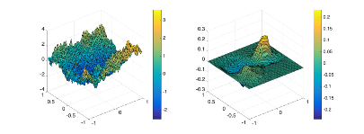
Refer to caption
Figure 2: Left: coefficient a(x)𝑎𝑥a(x) from SPE10 benchmark, in log10subscript10\log_{10} scale; Right: solution u𝑢u for the elliptic equation diva(x)u=sin(πx)sin(πy)div𝑎𝑥𝑢𝜋𝑥𝜋𝑦-\operatorname{div}a(x)\nabla u=\sin(\pi x)\sin(\pi y).
Refer to caption
Figure 3: Pre-wavelets ψ𝜓\psi at different scales.
Refer to caption
Figure 4: Solution for the elliptic equation with f=sin(πx)sin(πy)𝑓𝜋𝑥𝜋𝑦f=\sin(\pi x)\sin(\pi y).

We calculate the first 121212 eigenvalues using the multilevel correction method in Algorithm 4, therefore we actually take 𝔙(2)superscript𝔙2\mathfrak{V}^{(2)} as the coarsest subspace and the effective mesh size is H2=1/4superscript𝐻214H^{2}=1/4. We choose parameters m1=m2=2subscript𝑚1subscript𝑚22m_{1}=m_{2}=2 and p=1𝑝1p=1 in the multigrid iteration step defined in Algorithm 2 to solve the linear equation (3.36), and use Gauss-Seidel as the smoother.

We compare the gamblet based multilevel correction method with geometric multigrid multilevel correction method. In Table 1, we show the numerical results for the first 12 eigenvalues, here we take the number of subspace correction steps ϖ=1italic-ϖ1\varpi=1 for k=3,,q𝑘3𝑞k=3,\dots,q. For comparison, we also show the corresponding numerical results in Table 2 with the standard geometric multigrid linear solver. We observe much faster convergence for the gamblet based multilevel correction method (106superscript10610^{6} smaller for the first eigenvalue).

Table 1: Relative errors |(λi(k)λi)/λi|superscriptsubscript𝜆𝑖𝑘subscript𝜆𝑖subscript𝜆𝑖|(\lambda_{i}^{(k)}-\lambda_{i})/\lambda_{i}| for the gamblet based multilevel correction method, first a few iterations on the coarser levels

. i k = 2 k = 3 k = 4 k=5 k = 6 k = 7 1 6.1568e-2 1.3356e-2 3.0902e-3 1.2586e-3 3.8293e-4 1.5586e-8 2 1.6827e-1 3.0270e-2 4.6347e-3 1.0656e-3 2.4616e-4 5.3456e-8 3 7.9106e-1 1.1814e-1 2.3155e-2 2.8431e-3 2.9124e-4 4.7883e-6 4 5.8274e-1 1.9203e-1 4.5203e-2 7.7621e-3 7.7980e-4 4.4444e-5 5 7.5657e-1 1.6533e-1 1.6978e-2 2.8863e-3 3.3941e-4 1.0250e-5 6 9.4417e-1 2.9132e-1 5.0443e-2 7.0754e-3 7.7061e-4 4.4771e-5 7 1.7033e0 2.8337e-1 8.1393e-2 2.4187e-2 4.6014e-3 7.2897e-4 8 2.4517e0 5.0598e-1 1.3164e-1 2.4945e-2 4.6447e-3 8.7663e-4 9 6.4576e0 6.6654e-1 2.6205e-1 9.9177e-2 1.6962e-2 3.3086e-3 10 6.9955e0 6.8507e-1 2.4108e-1 4.7575e-2 1.9529e-2 9.6051e-3 11 1.0927e1 8.6987e-1 2.6043e-1 7.5851e-2 1.9996e-2 8.3358e-3 12 1.3665e1 9.5975e-1 3.3355e-1 5.9182e-2 1.9377e-2 7.5015e-3

Remark 4.1.

It is shown in [37] that for approximate eigenvalues with respect to the LOD coarse spaces on scale H𝐻H, a post-processing step can improve the eigenvalue error from H4superscript𝐻4H^{4} to H6superscript𝐻6H^{6}. The post-processing step is a correction with exact solve on the finest level. Since we are using an approximate solve in the correction step, this corresponds to the multilevel correction scheme with one correction step on each level, which is shown in Table 1. Comparing Table 1 with Table 2 in [37] shows a similar improvement of accuracy at the finer levels (although the coefficients a(x)𝑎𝑥a(x) are not the same, we expect a similar behavior for the approximation errors of eigenvalues). However, with geometric multigrid, the error reduction is very slow, which is shown by Table 2.

Table 2: Relative errors |(λi(k)λi)/λi|superscriptsubscript𝜆𝑖𝑘subscript𝜆𝑖subscript𝜆𝑖|(\lambda_{i}^{(k)}-\lambda_{i})/\lambda_{i}| for multilevel correction with geometric multigrid, first a few iterations on the coarser levels
i k = 2 k = 3 k = 4 k=5 k = 6 k = 7
1 2.6912e0 2.6698e0 2.5627e0 2.0948e0 4.4351e-1 5.0859e-2
2 2.4310e0 2.3886e0 2.3037e0 1.8812e0 4.8645e-1 5.4931e-2
3 2.3129e0 2.2749e0 2.1802e0 1.8076e0 4.9837e-1 6.4541e-2
4 2.6706e0 2.6225e0 2.5193e0 2.0636e0 5.8780e-1 9.2958e-2
5 3.1593e0 2.9673e0 2.8141e0 2.2948e0 6.2242e-1 9.8928e-2
6 2.7198e0 2.5764e0 2.4233e0 1.9427e0 5.3022e-1 7.5071e-2
7 2.9581e0 2.8158e0 2.6886e0 2.2162e0 6.1367e-1 9.9160e-2
8 2.9712e0 2.8012e0 2.6446e0 2.1981e0 6.4002e-1 9.3180e-2
9 3.7158e0 3.2765e0 3.0548e0 2.4382e0 6.8837e-1 1.1892e-1
10 3.1307e0 2.7671e0 2.5808e0 2.0749e0 5.9963e-1 8.4462e-2
11 3.0937e0 2.8429e0 2.6748e0 2.1673e0 5.7858e-1 8.8655e-2
12 3.1317e0 2.7967e0 2.6259e0 2.1068e0 5.8031e-1 8.6055e-2

If higher accuracy is pursued, we can take more correction steps at the finest level k=q𝑘𝑞k=q. See Figure 5 for the convergence history of both the gamblet based method and the geometric multigrid based method up to 1014superscript101410^{-14}. The gamblet based method converges much faster than the geometric multigrid based method.
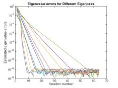
Refer to caption
Refer to caption
Figure 5: Convergence history for first 12 eigenvalues. Left: Gamblet based multilevel method Right: Geometric mutligrid based multilevel method. The iteration number corresponds to the number of correction steps, namely, the outer iteration number. The first a few iterations are on the coarse levels k=3,,q1𝑘3𝑞1k=3,\dots,q-1, and the following iterations are on the finest level k=q𝑘𝑞k=q.
Refer to caption
Figure 6: CPU time for Gamblet based multilevel correction and ARPACK

We now compare the efficiency of the multilevel correction method with the benchmark solver ARPACK (https://www.caam.rice.edu/software/ARPACK/). We implement the multilevel correction method in C (with a precomputed Gamblet decomposition), and run the code on a machine with two 6-core dual thread Intel Xeon E5-2620 2.00GHz CPUs with 72G memory. We solve for 12 eigenvalues, and stop the multilevel correction method when relative errors for all eigenvalues are below 109superscript10910^{-9}. For comparison, we use the ARPACK library to solve the same eigenvalue problems, and use the geometric multigrid method to solve the corresponding linear systems. The results in Figure 6 show that the Gamblet based multilevel correction method achieves a ten-fold acceleration in terms of CPU time. We only plot the “online” computing time for eigenpairs in Figure 6, the “offline” precomputing time for the Gamblet decomposition is not included since we only have a Matlab implementation for this part. For the Matlab implementation of the multilevel correction method, the running time for the “online” and “offline” parts are usually proportional, and the a priori theoretical bound on the complexity of the Gamblets precomputation is 𝒪(Nln2d+1N)𝒪𝑁superscript2𝑑1𝑁\mathcal{O}(N\ln^{2d+1}N).

4.2 Random Checkerboard

In the second example, we consider the eigenvalue problem for the random checkerboard case. Here, Ω=[1,1]×[1,1]Ω1111\Omega=[-1,1]\times[-1,1] and the matrix a(x)𝑎𝑥a(x) is a realization of random coefficients taking values 202020 or 1/201201/20 with probability 1/2121/2 at small scale ε=1/64𝜀164\varepsilon=1/64, see Figure 7. The coefficient a(x)𝑎𝑥a(x) has contrast 4×1024superscript1024\times 10^{2}, and is highly oscillatory.

We calculate the first 121212 eigenvalues. The parameters for Algorithm 4 are H=1/2𝐻12H=1/2, q=7𝑞7q=7, and we take 𝔙(2)superscript𝔙2\mathfrak{V}^{(2)} as the coarsest subspace. We choose m1=m2=2subscript𝑚1subscript𝑚22m_{1}=m_{2}=2 and p=1𝑝1p=1, and use Gauss-Seidel as the smoother in Algorithm 2. We take the number of subspace correction steps ϖ=1italic-ϖ1\varpi=1 for k=3,,q1𝑘3𝑞1k=3,\dots,q-1, then we run the subspace correction at the finest level k=q𝑘𝑞k=q until convergence.

Refer to caption
Figure 7: Random Checkerboard coefficient, in log10subscript10\log_{10} scale

The convergence rates shown in Figure 8 suggest a ten fold acceleration in terms of iteration number when comparing the gamblet and based multilevel correction method to the geometric multigrid based multilevel correction method. While it takes more than 800 iterations for geometric multigrid based multilevel correction method to converge for the first 12 eigenvalues to converge to accuracy 1014superscript101410^{-14}, the gamblet based multilevel correction method converges to that accuracy within 70 outer iterations.
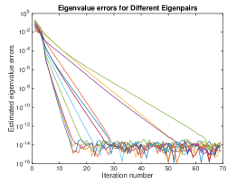
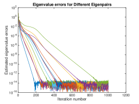
Refer to caption
Refer to caption
Figure 8: Convergence history for first 12 eigenvalues. Left: Gamblet based method Right: Geometric mutligrid based method. The iteration number corresponds to the number of correction steps, namely, the outer iteration number. The first a few iterations are on the coarse level k=3,,q1𝑘3𝑞1k=3,\dots,q-1, and the following iterations are on the finest level k=q𝑘𝑞k=q.

4.3 Gamblet Preconditioned LOBPCG Method

In the previous sections, we have proposed the Gamblet based multilevel correction scheme, proved its convergence and numerically demonstrated its performance. In this section, we will show that Gamblets can also be used as an efficient preconditioner for existing eigensolvers. To be precise, we construct the Gamblet based preconditioner for the Locally Optimal Block Preconditioned Conjugate Gradient (LOBPCG) method [25, 28], which is a class of widely used eigensolvers.

A variety of Krylov subspace-based methods are designed to solve a few extreme eigenvalues of symmetric positive matrix [49, 19, 10, 24, 25, 28, 7]. Many studies have shown that LOBPCG is one of the most effective method at this task [27, 18] and there are various recent developments of LOBPCG for indefinite eigenvalue problems [8], nonlinear eigenvalue problems [51], electronic structure calculation [52], and tensor decomposition [46]. The main advantages of LOBPCG are that the costs per iteration and the memory use are competitive with those of the Lanczos method, linear convergence is theoretically guaranteed and practically observed, it allows utilizing highly efficient matrix-matrix operations, e.g., BLAS 3, and it can directly take advantage of preconditioning, in contrast to the Lanczos method.

LOBPCG can be seen as a generalization of the Preconditioned Inverse Iteration (PINVIT) method [19, 10, 24]. The PINVIT method [19, 10, 24, 25, 28], can be motivated as an inexact Newton-method for the minimization of the Rayleigh quotient. The Rayleigh quotient μ(x)𝜇𝑥\mu(x) for a vector x𝑥x and a symmetric, positive definite matrix M𝑀M is defined by

μ(x,M):=μ(x)=xTMxxTxassign𝜇𝑥𝑀𝜇𝑥superscript𝑥𝑇𝑀𝑥superscript𝑥𝑇𝑥\mu(x,M):=\mu(x)=\frac{x^{T}Mx}{x^{T}x}

The global minimum of μ(x)𝜇𝑥\mu(x) is achieved at x=v1𝑥subscript𝑣1x=v_{1}, with λ1=μ(x)subscript𝜆1𝜇𝑥\lambda_{1}=\mu(x), where (λ1,v1)subscript𝜆1subscript𝑣1(\lambda_{1},v_{1}) is the eigenvalue pair of M𝑀M corresponding to the smallest eigenvalue λ1subscript𝜆1\lambda_{1}. This means that minimizing the Rayleigh quotient is equal to computing the smallest eigenvalue. With the following inexact Newton method:

wisubscript𝑤𝑖\displaystyle w_{i} =B1(Mxiμ(xi)xi),absentsuperscript𝐵1𝑀subscript𝑥𝑖𝜇subscript𝑥𝑖subscript𝑥𝑖\displaystyle=B^{-1}(Mx_{i}-\mu(x_{i})x_{i}),
xi+1subscript𝑥𝑖1\displaystyle x_{i+1} =xiwi.absentsubscript𝑥𝑖subscript𝑤𝑖\displaystyle=x_{i}-w_{i}.

we get the preconditioned inverse iteration (PINVIT). The preconditioner B𝐵B for M𝑀M have to satisfy IB1M􏱼􏱼Mc<1subscriptnorm𝐼superscript𝐵1𝑀􏱼􏱼𝑀𝑐1\|I-B^{-1}M\|_{􏱼􏱼M}\leq c<1. The inexact Newton method can be relaxed by adding a step size α𝛼\alpha

xi+1=xiαiwi,subscript𝑥𝑖1subscript𝑥𝑖subscript𝛼𝑖subscript𝑤𝑖x_{i+1}=x_{i}-\alpha_{i}w_{i},

Finding the optimal step size αisubscript𝛼𝑖\alpha_{i} is equivalent to solving the a small eigenvalue problem with respect to M𝑀M in the subspace {xi,wi}subscript𝑥𝑖subscript𝑤𝑖\{x_{i},w_{i}\}. In [25] Knyazev used the optimal vector in the subspace {xi1,wi,xi}subscript𝑥𝑖1subscript𝑤𝑖subscript𝑥𝑖\{x_{i-1},w_{i},x_{i}\} as the next iterate. The resulting method is called locally optimal (block) preconditioned conjugate method (LOBPCG).

In the following comparison, we adopt the Matlab implementation of LOBPCG by Knyazev [26]. We use the gamblet based multigrid as a preconditioner in the LOBPCG method, and compare its performance for SPE10 example with geometric multigrid preconditioned CG (GMGCG) and general purpose ILU based preconditioner, the results are shown in Figure 9. It is clear that the gamblet preconditioned LOBPCG as well as the gamblet multilevel correction scheme (see Figure 9) have better performance than the GMGCG or ILU preconditioned LOBPCG in terms of iteration number. The Gamblet based LOBPCG converges with the accuracy (residuals) of about 1015superscript101510^{-15}, with 56 iterations in about 30 seconds (in addition, the precomputation of the Gamblets costs about 18 seconds). While the GMG preconditioned LOBPCG in Figure 9 fails to converge in 1000 iterations, and the residuals are above 105superscript10510^{-5} when it is stopped at 1000 iterations in about 60 seconds. Although our implementation in Matlab is not optimized in terms of speed, the above observations indicate that the Gamblet preconditioned LOBPCG has potential to achieve even better performance with an optimized implementation.

Remark 4.2.

The LOBPCG method has a larger subspace for the small Rayleigh-Ritz eigenvalue problem, compared with the multilevel correction scheme in (3.37). This could be the reason why the gamblet preconditinoed LOBPCG scheme has fewer (but comparable) outer iterations compared with the multilevel correction scheme shown in Figure 5. On the other hand, orthogonalization is crucial for a robust implementation of LOBPCG, and adaptive stopping criteria needs to be used for efficiency. Delicate strategies [18] are proposed in order to ensure the robustness of LOBPCG. Comparing with LOBPCG, the Gamblet based multilevel correction scheme appears to be very robust in our numerical experiments: we only solve an eigenvalue problem at the coarsest level, and still achieve an accuracy of 1014superscript101410^{-14} without using any adaptive stopping criteria, for example, see Figure 5.
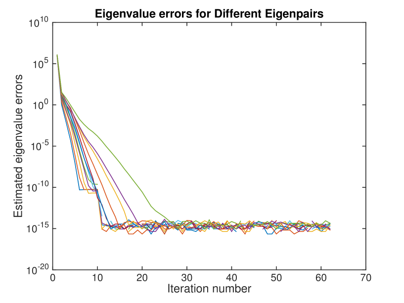
Refer to caption
(a) Eigenvalue errors for the gamblet preconditioned LOBPCG;
Refer to caption
(b) Residuals for the gamblet preconditioned LOBPCG;
Refer to caption
(c) Eigenvalue errors for the GMGCG preconditioned LOBPCG;
Refer to caption
(d) Residuals for the GMGCG preconditioned LOBPCG.
Refer to caption
(e) Eigenvalue errors for the ILU preconditioned LOBPCG;
Refer to caption
(f) Residuals for the ILU preconditioned LOBPCG.
Figure 9: Eigenvalue errors and residuals for the first 12 eigenpairs of the eigenvalue problems for SPE 10 case. Top row: Gamblet preconditioned LOBPCG. Middle row: geometric multigrid preconditioned LOBPCG. Bottom row: ILU preconditioned LOBPCG (using Matlab command ichol(A,struct(’michol’,’on’))).
Combination of Multilevel Correction with LOBPCG

We noticed that a “good” initial value is important for the convergence of the LOBPCG method. Therefore, we propose to combine the multilevel correction scheme and LOBPCG to derive a hybrid method. In this combination, the gamblet based multilevel correction scheme is used to compute, to a high accuracy, an initial approximation for the eigenpairs for the gamblet preconditioned LOBPCG scheme. We use this combined method to solve the so-called Anderson Localization eigenvalue problem in the following subsection. Since LOBPCG is based on the so-called Ky Fan trace minimization principle, at each step the sum of the eigenvalues are minimized [32]. Therefore the convergence rate of different eigenvalues will be balanced.

4.3.1 Anderson localization

Consider the linear Schrödinger operator :=Δ+V(x)assignΔ𝑉𝑥\mathcal{H}:=-\Delta+V(x) with disorder potential V(x)𝑉𝑥V(x) (as presented in [2]) whose Anderson localization [3] properties are analyzed in [4] and in [2] (see [9] and references therein for the ubiquity and importance of localization in wave physics).

Let Ω:=[1,1]2assignΩsuperscript112\Omega:=[-1,1]^{2} be the domain of the operator. By [2], V(x)𝑉𝑥V(x) is a disorder potential that vary randomly between two values β1ε2α𝛽1superscript𝜀2much-greater-than𝛼\displaystyle\beta\geq\frac{1}{\varepsilon^{2}}\gg\alpha on a small scale ε𝜀\varepsilon. In the numerical experiment, we choose ε=0.01𝜀0.01\varepsilon=0.01, β=104𝛽superscript104\beta=10^{4}, and α=1𝛼1\alpha=1 (the eigenvalue problem becomes more difficult as ε𝜀\varepsilon becomes smaller). See Figure 10 for results using the Gamblet based multilevel correction method, Gamblet preconditioned LOBPCG, and the hybrid method.
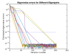
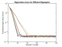
Refer to caption
Refer to caption
Refer to caption
Figure 10: Convergence history for first 12 eigenvalues: Left, using the gamblet based multilevel correction method; Middle: using the gamblet preconditioned LOBPCG method; Right, using the hybrid method, namely, generating the initial approximation by the gamblet based multilevel method, then preforming the gamblet preconditioned LOBPCG method until convergence. The iteration number corresponds to the number of correction steps, namely, the outer iteration number. The first a few iterations are on the coarse level k=3,,q1𝑘3𝑞1k=3,\dots,q-1, and the following iterations are on the finest level k=q𝑘𝑞k=q.

Acknowledgement

HX was partially supported by Science Challenge Project (No. TZ2016002), National Natural Science Foundations of China (NSFC 11771434, 91330202), the National Center for Mathematics and Interdisciplinary Science, CAS. LZ was partially supported by National Natural Science Foundations of China (NSFC 11871339, 11861131004, 11571314). HO gratefully acknowledge support from the Air Force Office of Scientific Research and the DARPA EQUiPS Program under award number FA9550-16-1-0054 (Computational Information Games) and the Air Force Office of Scientific Research under award number FA9550-18-1-0271 (Games for Computation and Learning). We thank Florian Schaefer for stimulating discussions. We thank two anonymous reviewers whose comments have greatly improved this manuscript.

References

  • [1] R. A. Adams and J. Fournier. Sobolev spaces, volume 140 of Pure and Applied Mathematics (Amsterdam). Elsevier/Academic Press, Amsterdam, second edition, 2003.
  • [2] R. Altmann, P. Henning, and D. Peterseim. Quantitative anderson localization of schrödinger eigenstates under disorder potentials. arXiv:1803.09950, 2018.
  • [3] P. W. Anderson. Absence of diffusion in certain random lattices. Phys. Rev., 109:1492–1505, 1958.
  • [4] D. N. Arnold, G. David, D. Jerison, S. Mayboroda, and M. Filoche. Effective confining potential of quantum states in disordered media. PRL, 116:056602, 2016.
  • [5] I. Babuška and J. Osborn. Finite element-galerkin approximation of the eigenvalues and eigenvectors of selfadjoint problems. Math. Comp., 52:275–297, 1989.
  • [6] I. Babuška and J. Osborn. Eigenvalue problems. In P. G. Lions and Ciarlet P.G., editors, Handbook of Numerical Analysis, Vol. II, Finite Element Methods (Part 1), chapter Eigenvalue Problems, pages 641–787. North-Holland, Amsterdam, 1991.
  • [7] Z. Bai, J. Demmel, J. Dongarra, A. Ruhe, and H. van der Vorst, editors. Templates for the Solution of Agebraic Eigenvalue Problems: A Practical Guide. Society for Industrial and Applied Math., Philadelphia, 2000.
  • [8] Z. Bai and R. C. Li. Minimization principles for the linear response eigenvalue problem i: theory. SIAM J. Matrix Anal. Appl., 33(4):1075–1100, 2012.
  • [9] J. Billy, V. Josse, Z. Zuo, A. Bernard, B. Hambrecht, P. Lugan, D.Clément, L. Sanchez-Palencia, P. Bouyer, and A. Aspect. Direct observation of anderson localization of matter waves in a controlled disorder. Nature, 453:891–894, 2008.
  • [10] J. Bramble, J. Pasciak, and A. Knyazev. A subspace preconditioning algorithm for eigenvector/eigenvalue computation. Advances in Computational Mathematics, 6(1):159–189, 1996.
  • [11] A. Brandt. Multi-level adaptive technique (MLAT) for fast numerical solutions to boundary value problems. In Proc. 3rd Int’l Conf. Numerical Methods in Fluid Mechanics, 1973. Lecture Notes in Physics 18.
  • [12] Susanne C Brenner, Peter Monk, and Jiguang Sun. C0 ipg method for biharmonic eigenvalue problems. In Academy of Mathematics and Systems Science, CAS Colloquia & Seminars, 2014.
  • [13] M. E. Brewster and G. Beylkin. A multiresolution strategy for numerical homogenization. Appl. Comput. Harmon. Anal., 2(4):327–349, 1995.
  • [14] L. Cao and J. Cui. Asymptotic expansions and numerical algorithms of eigenvalues and eigenfunctions of the dirichlet problem for second order elliptic equations in perforated domains. Numer. Math., 96:525–581, 2004.
  • [15] F. Chatelin. Spectral Approximation of Linear Operators. Academic Press Inc, New York, 1983.
  • [16] H. Chen, H. Xie, and F. Xu. A full multigrid method for eigenvalue problems. J. Comput. Phys, 322:747–759, 2016.
  • [17] M. Dorobantu and B. Engquist. Wavelet-based numerical homogenization. SIAM J. Numer. Anal., 35(2):540–559 (electronic), 1998.
  • [18] J. A. Duersch, M. Shao, C. Yang, and M. Gu. A robust and efficient implementation of lobpcg. SIAM J. Sci. Comput., 40(5):C655–C676, 2018.
  • [19] E. G. D’yakonov and M. Yu. Orekhov. Minimization of the computational labor in determining the first eigenvalues of differential operators. Math. Notes, 27:382–391, 1980.
  • [20] W. Hackbusch. A fast iterative method for solving Poisson’s equation in a general region. In Numerical treatment of differential equations (Proc. Conf., Math. Forschungsinst., Oberwolfach, 1976), pages 51–62. Lecture Notes in Math., Vol. 631. Springer, Berlin, 1978.
  • [21] T. Y. Hou, D. Huang, K. C. Lam, and Z. Zhang. A fast hierarchically preconditioned eigensolver based on multiresolution matrix decomposition. arXiv:1804.03415, 2018.
  • [22] T. J. R. Hughes, G. R. Feijóo, L. Mazzei, and J.-B. Quincy. The variational multiscale method—a paradigm for computational mechanics. Computer Methods in Applied Mechanics and engineering, 166(1-2):3–24, 1998.
  • [23] S. Jia, H. Xie, M. Xie, and F. Xu. A full multigrid method for nonlinear eigenvalue problems. Sci. China Math., 59:2037–2048, 2016.
  • [24] A. Knyazev. Preconditioned eigensolvers - an oxymoron? Electronic Transactions on Numerical Analysis, 7:104–123, 1998.
  • [25] A. Knyazev. Toward the optimal preconditioned eigensolver: Locally optimal block preconditioned conjugate gradient method. SIAM Journal on Scientific Computing, 23(2):517–541, 2001.
  • [26] A. Knyazev. lobpcg.m, https://www.mathworks.com/matlabcentral/fileexchange/48-lobpcg-m, 2015. Version 1.5.
  • [27] A. Knyazev. Recent implementations, applications, and extensions of the locally optimal block preconditioned conjugate gradient method (lobpcg). arXiv:1708.08354, 2017.
  • [28] A. Knyazev and K. Neymeyr. Efficient solution of symmetric eigenvalue problems using multigrid preconditioners in the locally optimal block conjugate gradient method. Electronic Transactions on Numerical Analysis., 15:38–55, 2003.
  • [29] W. Kohn. Analytic properties of Bloch waves and Wannier functions. Physical Review, 115(4):809, 1959.
  • [30] R. Kornhuber, D. Peterseim, and H. Yserentant. An analysis of a class of variational multiscale methods based on subspace decomposition. Math. Comp., 87:2765–2774, November 2018. Submitted for publication.
  • [31] R. Kornhuber and H. Yserentant. Numerical homogenization of elliptic multiscale problems by subspace decomposition. Multiscale Model. Simul., 14(3):1017–1036, 2016.
  • [32] D. Kressner, M. Pandur, and M. Shao. An indefinite variant of lobpcg for definite matrix pencils. Numerical Algorithms, 66(4):681–703, 2014.
  • [33] R. Kyng and S. Sachdeva. Approximate gaussian elimination for laplacians: Fast, sparse, and simple. FOCS, 2016.
  • [34] Q. Lin and H. Xie. An observation on aubin-nitsche lemma and its applications. Mathematics in Practice and Theory, 41(17):247–258, 2011.
  • [35] Q. Lin and H. Xie. A multilevel correction type of adaptive finite element method for steklov eigenvalue problems. In Proceedings of the International Conference Applications of Mathematics, pages 134–143, 2012.
  • [36] Q. Lin and H. Xie. A multi-level correction scheme for eigenvalue problems. Math. Comp., 84:71–88, 2015.
  • [37] A. Målqvist and D. Peterseim. Computation of eigenvalues by numerical upscaling. Numer. Math., 130(2):337–361, 2014.
  • [38] A. Målqvist and D. Peterseim. Localization of elliptic multiscale problems. Mathematics of Computation, 83(290):2583–2603, 2014.
  • [39] C. A. Micchelli and T. J. Rivlin. A survey of optimal recovery. In Optimal Estimation in Approximation Theory, pages 1–54. Springer, 1977.
  • [40] M. Olshanskii and E. Tyrtyshnikov. Iterative Methods for Linear Systems - Theory and Applications. SIAM, 2014.
  • [41] H. Owhadi. Multigrid with rough coefficients and multiresolution operator decomposition from hierarchical information games. SIAM Rev., 59(1):99–149, March 2017.
  • [42] H. Owhadi and C. Scovel. Universal scalable robust solvers from computational information games and fast eigenspace adapted multiresolution analysis. arXiv:1703.10761, 2017.
  • [43] H. Owhadi and C. Scovel. Operator adapted wavelets, fast solvers, and numerical homogenization from a game theoretic approach to numerical approximation and algorithm design. Cambridge University Press, 2019. Cambridge Monographs on Applied and Computational Mathematics.
  • [44] H. Owhadi and L. Zhang. Gamblets for opening the complexity-bottleneck of implicit schemes for hyperbolic and parabolic odes/pdes with rough coefficients. J. Comput. Phys., 347:99–128, 2017.
  • [45] H. Owhadi, L. Zhang, and L. Berlyand. Polyharmonic homogenization, rough polyharmonic splines and sparse super-localization. ESAIM Math. Model. Numer. Anal., 48(2):517–552, 2014.
  • [46] M. Rakhuba and I. Oseledets. Calculating vibrational spectra of molecules using tensor train decomposition. J. Chem. Phys., 145:124101, 2016.
  • [47] Y. Saad. Numerical Methods For Large Eigenvalue Problems. SIAM, 2011.
  • [48] F. Schäfer, T. J. Sullivan, and H. Owhadi. Compression, inversion, and approximate PCA of dense kernel matrices at near-linear computational complexity. arXiv:1706.02205, 2017.
  • [49] D. Sorensen. Implicitly Restarted Arnoldi/Lanczos Methods for Large Scale Eigenvalue Calculations. Springer Netherlands, 1997.
  • [50] G. Strang and G. Fix. An analysis of the finite element method. Prentice‐Hall, 1973.
  • [51] D. B. Szyld and F. Xue. Preconditioned eigensolvers for large-scale nonlinear hermitian eigenproblems with variational characterizations. i. external eigenvalues. Mathematics of Computation, 85:2887–2918, 2016.
  • [52] E. Vecharynski, C. Yang, and J. E.Pask. A projected preconditioned conjugate gradient algorithm for computing many extreme eigenpairs of a hermitian matrix. Journal of Computational Physics, 290:73–89, 2015.
  • [53] W. L. Wan, Tony F. Chan, and Barry Smith. An energy-minimizing interpolation for robust multigrid methods. SIAM J. Sci. Comput., 21(4):1632–1649, 1999/00.
  • [54] G. H. Wannier. Dynamics of band electrons in electric and magnetic fields. Reviews of Modern Physics, 34(4):645, 1962.
  • [55] H. Xie. A multigrid method for eigenvalue problem. J. Comput. Phys., 274:550–561, 2014.
  • [56] H. Xie. A type of multilevel method for the steklov eigenvalue problem. IMA J. Numer. Anal., 34:592–608, 2014.
  • [57] J. Xu and A. Zhou. A two-grid discretization scheme for eigenvalue problems. Mathematics of Computation, 70(233):17–25, 2001.
  • [58] Gene Ryan Yoo and Houman Owhadi. De-noising by thresholding operator adapted wavelets. Statistics and Computing, 2019.
  • [59] L. Zhang, L. Cao, and X. Wang. Multiscale finite element algorithm of the eigenvalue problems for the elastic equations in composite materials. Comput. Methods Appl. Mech. Engrg., 198:2539–2554, 2009.
  • [60] Shuo Zhang, Yingxia Xi, and Xia Ji. A multi-level mixed element method for the eigenvalue problem of biharmonic equation. Journal of Scientific Computing, pages 1–30, 2017.