Bayesian approach to model-based extrapolation of nuclear observables

Abstract

Background

The mass, or binding energy, is the basis property of the atomic nucleus. It determines its stability, and reaction and decay rates. Quantifying the nuclear binding is important for understanding the origin of elements in the universe. The astrophysical processes responsible for the nucleosynthesis in stars often take place far from the valley of stability, where experimental masses are not known. In such cases, missing nuclear information must be provided by theoretical predictions using extreme extrapolations. In order to take full advantage of the information contained in mass model residuals, i.e., deviations between experimental and calculated masses, one can utilize Bayesian machine learning techniques to improve predictions.

Purpose

In order to improve the quality of model-based predictions of nuclear properties of rare isotopes far from stability, we consider the information contained in the residuals in the regions where the experimental information exist. As a case in point, we discuss two-neutron separation energies $S_{2n}$ of even-even nuclei. Through this observable, we assess the predictive power of global mass models towards more unstable neutron-rich nuclei and provide uncertainty quantification of predictions.

Methods

We consider 10 global models based on nuclear Density Functional Theory with realistic energy density functionals as well as two more phenomenological mass models. The emulators of $S_{2n}$ residuals and credibility intervals (Bayesian confidence intervals) defining theoretical error bars are constructed using Bayesian Gaussian processes and Bayesian neural networks. We consider a large training dataset pertaining to nuclei whose masses were measured before 2003. For the testing datasets, we considered those exotic nuclei whose masses have been determined after 2003. By establishing statistical methodology and parameters, we carried out extrapolations towards the $2n$ dripline.

Results

While both Gaussian processes and Bayesian neural networks reduce the rms deviation from experiment significantly, GP offers a better and much more stable performance. The increase in the predictive power of microscopic models aided by the statistical treatment is quite astonishing: the resulting rms deviations from experiment on the testing dataset are similar to those of more phenomenological models. We found that Bayesian neural networks results are prone to instabilities caused by the large number of parameters in this method. Moreover, since the classical sigmoid activation function used in this approach has linear tails that do not vanish, it is poorly suited for a bounded extrapolation. The empirical coverage probability curves we obtain match very well the reference values, in a slightly conservative way in most cases, which is highly desirable to ensure honesty of uncertainty quantification. The estimated credibility intervals on predictions make it possible to evaluate predictive power of individual models, and also make quantified predictions using groups of models.

Conclusions

The proposed robust statistical approach to extrapolation of nuclear model results can be useful for assessing the impact of current and future experiments in the context of model developments. The new Bayesian capability to evaluate residuals is also expected to impact research in the domains where experiments are currently impossible, for instance in simulations of the astrophysical $r$-process.

I Introduction

The knowledge of nuclear binding energy is of fundamental importance for basic science and applications. Nuclear masses define the extent and details of the nuclear landscape, determine nuclear stability and decay channels, as well as decay and reaction rates. Precision measurements of nuclear masses and moments are needed for tests of fundamental symmetries of nature. In many cases, however, mass measurements are not practically possible and the missing information must be provided by theoretical models of nuclear structure. A good example is in the astrophysical $r$-process that involve neutron-rich, short-lived nuclei that cannot be accessed experimentally in the foreseeable future.

Theoretically, there has been noticeable progress in global modeling of nuclear masses and other nuclear properties. A microscopic approach that is well suited to providing quantified predictions throughout the nuclear chart is nuclear Density Functional Theory (DFT) Bender et al. (2003). An effective interaction in DFT is given by the energy density functional (EDF), whose coupling constants are adjusted to measured observables Bender et al. (2003); Erler et al. (2012); Goriely et al. (2013, 2016); Kortelainen et al. (2014); Afanasjev et al. (2015); Afanasjev and Agbemava (2016); Wang and Chen (2015); Xia et al. (2018). This global approach can be used to assess the uncertainties on calculated observables, both statistical and systematic Dobaczewski et al. (2014); McDonnell et al. (2015). Such a capability is essential, especially in the context of making wide-ranging extrapolations into the regions where experiments are impossible.

A basic test of any EDF parameterization is its ability to reproduce measured binding energies and other nuclear properties across the nuclear chart. Typically, the commonly used EDFs yield overall root-mean-square (rms) deviations between theoretical and experimental masses in the range from 1 to 5 MeV Kortelainen et al. (2014); Afanasjev and Agbemava (2016). Currently, the best overall agreement with experimental masses (rms deviation of 0.56 MeV) is obtained with the HFB-31 model of Ref. Goriely et al. (2016), which is rooted in the Skyrme EDF. However, this excellent result has been obtained at a price of several phenomenological corrections adjusted to the data.

In the context of many structural and astrophysical applications, the challenge is to carry out reliable model-based extrapolations into the regions where experimental data are not available. Recently, a critical assessment of the predictive power of various mass models was performed in Ref. Sobiczewski and Litvinov (2014). They did not find a correlation between a model’s calibration (measured in terms of a rms mass deviation) and its ability to predict new masses. Indeed, if a model is merely a many-parameter formula fitted to experimental data, i.e., it does not have a sound microscopic foundation, it cannot be expected to provide sound predictions when it comes to major extrapolations outside the known regions.

In this paper, we investigate the predictive power of current global nuclear models with respect to two-neutron ($2n$) separation energies $S_{2n}(Z,N)$ of even-even nuclei. The neutron separation energy is a basic structural observable that determines the position of the neutron dripline, $r$-process trajectory, and – in general – is a strong indicator of nuclear shell effects and correlations. Theoretically, $S_{2n}(Z,N)$ is an observable that is safer to predict than the binding energy. Indeed, in most cases, deviations between computed and experimental values of $S_{2n}(Z,N)$ are significantly reduced as compared to mass residuals Kortelainen et al. (2012). This better prediction (lower residuals) in separation energies is to be expected as many systematic model uncertainties in the binding energy cancel out in binding energy differences. Here and throughout, we use the term “residual” to denote the difference between an experimental value and a model prediction, as can be seen in definition (1) below. We limit our study to even-even nuclei as we want to avoid additional complications and uncertainties related to the choice and treatment of quasi-particle configurations in odd-$A$ and odd-odd systems Bonneau et al. (2007); Schunck et al. (2010); Afanasjev (2015).

When the experimental two-neutron separation energies $S_{2n}^{\mathrm{exp}}(Z,N)$ are known, they can be related to the model predictions $S_{2n}^{\mathrm{th}}(Z,N,\vartheta)$ via:

$$S_{2n}^{\mathrm{exp}}(Z,N)=S_{2n}^{\mathrm{th}}(Z,N,\vartheta)+\delta(Z,N),$$ (1)

where $\vartheta$ is the vector representing all model parameters and $\delta(Z,N)$ is the separation-energy residual we were just discussing. The problem at hand is to calibrate the model (i.e., estimate $\vartheta$), calculate the separation energies inside and outside the range of experimental data, and estimate the uncertainty on predictions.

The residual $\delta(Z,N)$ contains a systematic component due to missing aspects in the modeling (simplifications, incorrect assumptions, incomplete physics, etc.) and the statistical component stemming from experimental errors and uncertainties on model parameters $\vartheta$ resulting from the model optimization process. In the following, we shall disregard the experimental errors on separation energies as those are usually well below theoretical uncertainties.

In many current applications, the statistical uncertainty has been estimated by means of classical linear regression techniques Dobaczewski et al. (2014); Gao et al. (2013); Goriely and Capote (2014); Kortelainen (2015); Nikšić et al. (2015); Haverinen and Kortelainen (2017) or Bayesian inference methods McDonnell et al. (2015); Schunck et al. (2015), the latter typically sharing the same spirit as classical techniques from a modeling standpoint. We will have more to say in Section IV about how the Bayesian context distinguishes itself. Systematic errors, seen in the distribution of residuals as trends, or patterns, are extremely difficult to estimate as the exact model is not available. The systematic uncertainty on separation energies is often estimated by an analysis of inter-model dependences. In the context of nuclear masses, this has been done by comparing predictions of different DFT frameworks and different EDF parametrizations Erler et al. (2012); Afanasjev et al. (2015); Wang and Chen (2015); Xia et al. (2018).

One can improve a theory’s predictive power by comparing model predictions to existing data. Here, a powerful strategy is to estimate residuals by developing an emulator for $\delta(Z,N)$ using a training set of known masses. An emulator $\delta^{\mathrm{em}}(Z,N)$ can, for instance, be constructed by employing Bayesian approaches, such as Gaussian processes, neural networks, and frequency-domain bootstrap Athanassopoulos et al. (2004); Bayram et al. (2014); Bayram and Akkoyun (2017); Yuan (2016); Utama et al. (2016a); Utama and Piekarewicz (2017, 2018); Bertsch and Bingham (2017); Zhang et al. (2017); Niu and Liang (2018). The unknown separation energies can then be estimated from Eq. (1) by combing theoretical predictions and estimated residuals:

$$S_{2n}^{\mathrm{est}}(Z,N)=S_{2n}^{\mathrm{th}}(Z,N,\vartheta)+\delta^{\mathrm{em}}(Z,N).$$ (2)

It is worth noting that by developing reliable emulators $\delta^{\mathrm{em}}(Z,N)$, which take into account correlations between masses of different nuclei, one can significantly refine mass predictions and estimate uncertainties on predicted values Utama and Piekarewicz (2017); Zhang et al. (2017); Niu and Liang (2018). Moreover, since the surface of residuals $\delta(Z,N)$ contains important insights about model deficiencies, by studying the patterns of $\delta^{\mathrm{em}}(Z,N)$ one can make progress in developing higher-fidelity models.

The paper is organized as follows. Section II lists the mass models and experimental datasets used in our tests. The statistical methodology adopted in our work is outlined in Sec. III. The statistical Gaussian process and Bayesian neural network frameworks employed to construct $\delta^{\mathrm{em}}(Z,N)$ are described in Sec. IV. The results are presented in Sec. V, which also contains the analysis of advantages and disadvantages of different statistical strategies in the context of previous work. In particular, Sec. V.3 studies the statistically corrected predictions of the models beyond the range of available data and discusses their reliability. In Sec. V.4 we discuss some numerical implementation challenges related to the calibration of neural networks. Finally, Sec. VI presents conclusions and perspectives for future studies.

II Nuclear Models

In the context of meaningful extrapolations in the neutron excess $N-Z$ and/or mass $A$, any underlying theoretical mass model we choose to use should meet several criteria. First, since such a model is meant to be used in the regions of the nuclear landscape far from the regions of known masses, it should be based on controlled many-body formalism employing quantified input (interaction, energy functional). Second, the theoretical framework should be capable of reproducing basic nuclear properties impacting nuclear masses (such as shell structure and deformations). Finally, the model should be globally applicable throughout the nuclear chart. For these reasons, we eliminate from our considerations phenomenological multi-parameter mass formulae, such as Koura et al. (2005); Duflo and Zuker (1995) which are directly fitted to experimental data.

The models used and evaluated in this study can be divided into three groups. The first group contains global mass models FRDM-2012 Möller et al. (2016) and HFB-24 Goriely et al. (2013) which are commonly used in astrophysical nucleosynthesis network simulations. The FRDM is a representative of well-fitted microscopic-macroscopic mass models. The model HFB-24 is rooted in a self-consistent mean-field approach with several phenomenological corrections added. For both models, the rms deviation from experimental masses is around 0.6 MeV. As explained in the introduction, this is about as low as one can expect without running into having to make uncomfortably many phenomenological corrections.

The second group contains six microscopic Skyrme-DFT models based on realistic energy density functionals SkM^∗ Bartel et al. (1982), SkP Dobaczewski et al. (1984), SLy4 Chabanat et al. (1995), SV-min Klüpfel et al. (2009), UNEDF0 Kortelainen et al. (2010), and UNEDF1 Kortelainen et al. (2012). For these models, the rms mass deviation typically ranges from 1.5 MeV (UNEDF0) to $\sim$5 MeV (SLy4) Kortelainen et al. (2012).

The third group contains four microscopic covariant-DFT models based on realistic relativistic energy density functionals NL3^∗ Lalazissis et al. (2009), DD-ME2 Lalazissis et al. (2005), DD-PC1 Nikšić et al. (2008), DD-ME$\delta$ Roca-Maza et al. (2011). Here, the rms mass deviation varies between 2 and 3 MeV Afanasjev and Agbemava (2016). The predictions of the second and third group of models can be found in the theoretical database MassExplorer mas .

The solutions of DFT equations corresponding to localized densities exist only for the neutron chemical potential $\lambda_{n}<0$ (or $S_{2n}>0$). For $\lambda_{n}>0$, the nucleus is formally unbound and the standard DFT solution is not meaningful Dobaczewski and Nazarewicz (2013); Michel et al. (2008). The $2n$ dripline, $S_{2n}=0$, is formally reached for $\lambda_{n}=0$ Erler et al. (2012). Consequently, the DFT predictions discussed here are terminated when $\lambda_{n}$ becomes positive.

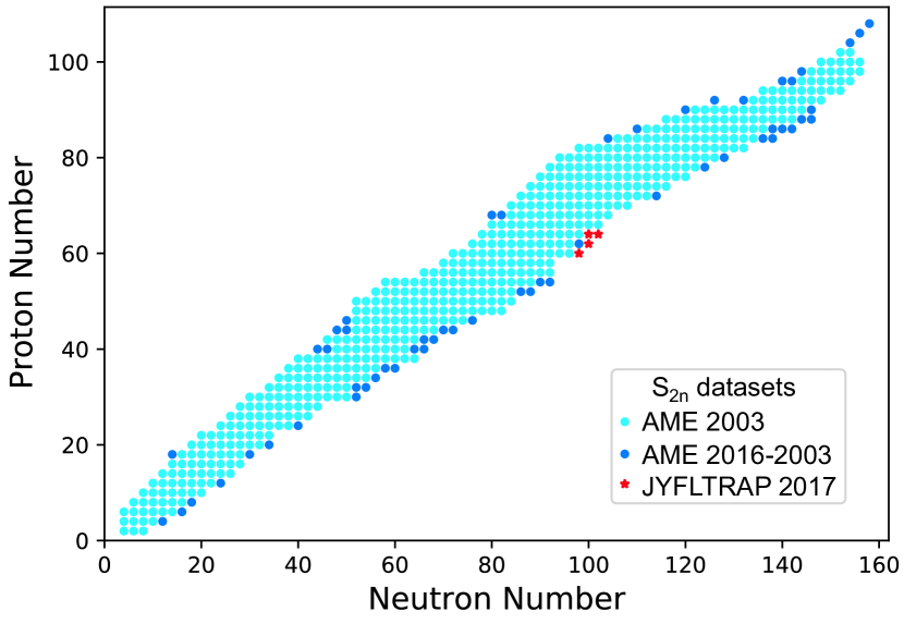
Figure 1: The experimental $S_{2n}(Z,N)$ datasets for even-even nuclei used in our study: AME2003 Wapstra et al. (2003); Audi et al. (2003) (light dots, 537 points), additional data that appeared in the AME2016 evaluation Huang et al. (2017); Wang et al. (2017) (dark dots, 55 points), and JYFLTRAP Vilen et al. (2018) (stars, 4 points).

In order to assess the predictive power of nuclear mass models, for the training dataset used in Sec. V.1, we take 537 values of $S_{2n}^{\mathrm{exp}}(Z,N)$ from the AME2003 mass evaluation Wapstra et al. (2003); Audi et al. (2003). As discussed in Ref. Sobiczewski and Litvinov (2014), nuclear mass models based on the mean-field approach perform generally better in heavier nuclei. Consequently, to test the performance of our statistical models in heavier nuclei, we also consider the training dataset AME2003-H obtained by removing the data on lighter nuclei below $Z<20$ from the original AME2003 dataset Utama et al. (2016a); Utama and Piekarewicz (2017, 2018). The resulting emulators $\delta^{\mathrm{em}}(Z,N)$ are then used to predict 55 new data points that appeared in the AME2016 mass evaluation Huang et al. (2017); Wang et al. (2017), thereby allowing us to test these predictions as explained in Sec. V.1. This joint dataset is referred to as AME2016-AME2003 in the following. In Sec. V.2 we also employed the AME2016-H training dataset ($Z<20$ data removed from AME2016) to test model predictions for 4 points that have been measured very recently at the JYFLTRAP Penning trap Vilen et al. (2018).

The ranges of experimental data used in this study are shown in Fig. 1. It is to be noted that the mass models employed in this work were optimized to subsets of the masses listed in the training set AME2003. The only exception is HFB-24, which has also used additional AME2016-AME2003 data listed in the evaluation AME2012 Wang et al. (2012).

Before moving on to our predictive methodology and results, we describe a visual inspection of the data. The $S_{2n}(Z,N)$ residuals (1) for the global mass models UNEDF1, SLy4, DD-ME2, DD-PC1, FRDM-2012, and HFB-24 are shown in Fig. 2. Long-range patterns are clearly visible atop the fluctuating background, which can be interpreted as statistical noise. To better recognize these systematic trends, we smoothed out the residuals with a Gaussian folding function in $(Z,N)$, see Fig. 3. The substantial deviations between experiment and theory around neutron magic numbers Kortelainen et al. (2010); Gao et al. (2013) are noticeable. Those are most likely related to an inferior description of the ground-state collective correlation energies Bender et al. (2006); Delaroche et al. (2010); Carlsson et al. (2013). The magnitude and sign of systematic trends in $\delta^{\mathrm{em}}(Z,N)$ is model-dependent. While the more phenomenological models FRDM-2012 and HFB-24, primarily fitted to the large mass dataset AME2003, provide a very good reproduction of experimental values, some long-range deviations are still present. The models SLy4, DD-ME2, and DD-PC1 exhibit the largest deviations around the neutron magic gaps, usually attributed to their low effective masses Agbemava et al. (2014); Kortelainen et al. (2010). The UNEDF1 model exhibits fairly smooth systematic trends, with the largest deviations around $N=126$.

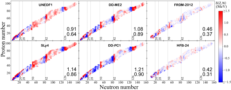
Figure 2: Residuals of $S_{2n}(Z,N)$ for the six global mass models with respect to the testing dataset AME2003. The rms values of $\delta(Z,N)$ in MeV are marked: for AME2003 (upper number) and AME2003-H (lower number)

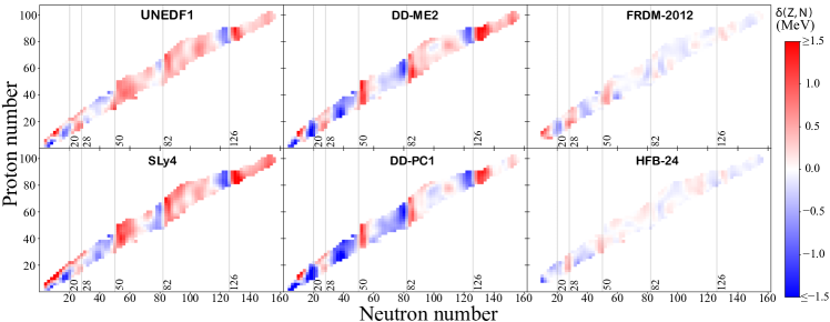
Figure 3: Similar as in Fig. 2 but for $S_{2n}(Z,N)$ residuals smoothed with the Gaussian folding function to emphasize long-range systematic trends.

III Statistical Methodology

III.1 Bayesian approach

A Bayesian methodology can be understood as a statistical solution to a simple ill-posed inverse problem, when the problem is based on a set of probability models. In this framework, a model is given which relates observations to unknown parameters and variables, and contains a term representing the statistical errors. The model is typically set up as an explanation of the observations from the unknown parameters and variables, and the question is to invert the model, i.e., to predict the unknowns from the observations. Since inverting this equation is an ill-posed problem (too much data, usually far too much, to determine a unique solution), one must first admit that the equation contains a noise term, defined in probabilistic terms (using random variables), in which case one calls it a likelihood equation. To provide a systematical solution which is consistent with the notion of conditional probability, the Bayesian framework resorts to external information , or beliefs, about the unknowns: these are probability models, known as the priors, for each of the unknown parameters and for any unknown variables to be predicted. The output of the Bayesian analysis is a set of probability densities or distributions, known as the posteriors. In this sense, the Bayesian approach provides statistical estimators of all parameters and variables to be predicted. More precisely, each posterior is a full description of the uncertainty surrounding each unknown, and in principle, surrounding all the unknowns jointly (simultaneously) as a group, each posterior mean value being interpreted as an estimator. Just like in most prediction activities, the predictive ability of Bayesian approach, based on training data, lies in the flexibility to first estimate parameters by comparing predicted variables to known observations, and then use those estimates to make other predictions in domains where no training data are available. It is important to note that the Bayesian inversion we just described takes on a particularly simple form, which makes it computationally attractive.

We perform a fully Bayesian analysis of the residuals $\delta(Z,N)$ with two different classes of statistical models: Gaussian processes (GP), and Bayesian neural networks (BNN). By “fully Bayesian”, we mean that we investigate the actual posterior distributions of all predicted quantities, and all statistical model parameters. We do not attempt to incorporate any frequentist analysis within the Bayesian framework, contrary to what is occasionally done, in particular for GP (see, e.g., Ref. Kennedy and O’Hagan (2001)). In this fashion, the full probabilistic interpretation of the Bayesian output is legitimately preserved. Each of the two classes of statistical models has its own strength: GP has ability to take advantage of short-range correlations, and BNN is expected to capture long-range trends.

Whether GP or BNN, the statistical model relates the particle numbers $(Z,N)$ to a corresponding observed residual $\delta\left(Z,N\right)$ in the region where data are available to train predictions. Let us fix these ideas by introducing some generic notation. We will denote each statistical model class by a function $f$ of the particle numbers $\left(Z,N\right)$, depending on parameters $\theta$ which are unknown and must be estimated. Thus, denoting $x_{i}:=(Z,N)$ and $y_{i}:=\delta(Z,N)$ for a nucleus label $i$, our Bayesian model is of the form:

$$y_{i}=f(x_{i},\theta)+\sigma\epsilon_{i},$$ (3)

where $f$ is either GP or BNN with parameters $\theta$, and the error is modeled as a random variable $\epsilon_{i}$ which is added to the relation. In general, $f$ can either be a deterministic function, or a random variable itself. In our GP application described in Sec. IV.1, $f$ will be a random variable. For the BNN, $f$ is non-random. We assume that the $\epsilon_{i}$ are independent standard Gaussian variables (mean zero and unit variance), and $\sigma$ is a noise scale parameter. The relation (3) is called the likelihood equation, because it relates the data $y_{i}$ with unknown parameters $\theta$ and $\sigma$. We denote the probability density of $y$ in the likelihood model by $p(y|\theta,\sigma)$, assuming fixed $\theta$ and $\sigma$. In regions of $x_{i}$ where the values of $y_{i}$ are unknown, we can use (3) to predict them. We must also assume prior distributions on the unknown parameters, e.g., a joint probability density $\pi(\theta,\sigma)$.

Bayes’ theorem states that the posterior density of $(\theta,\sigma)$ given the data for $y$, under the prior and likelihood models, is proportional to the product of the likelihood density of $y$ given $(\theta,\sigma)$ and the prior density of $(\theta,\sigma)$:

$$p(\theta,\sigma|y)\propto p(y|\theta,\sigma)\pi(\theta,\sigma).$$ (4)

We can also compute predictions $y^{\ast}$ in the regions of $x$ where the corresponding $y$ is not observed. This simply requires computing the conditional density of $y^{\ast}$ given $y,\theta,\sigma$, where $y$ is in known regions, and integrating over the posterior density of the unknown parameters from (4):

$$p(y^{\ast}|y)=\int p(y^{\ast}|y,\theta,\sigma)p(\theta,\sigma|y)\,d\theta d\sigma.$$ (5)

Typically, and certainly in our case, the conditional probability $p(y^{\ast}|y,\theta,\sigma)$ is given explicitly from a direct examination of the likelihood model (3). When an assumption is made in (3) by which the components of (3) are independent of each other for each $x_{i}=\left(Z,N\right)$, then $p(y^{\ast}|y,\theta,\sigma)$ does not depend explicitly on $y$. In the GP case, even though the additive errors terms $\epsilon_{i}$ are independent, the components of $f(x,\theta)$ are not, because the $(Z,N)$ landscape is viewed as a spatial index where nearby nuclei must be highly correlated, as we will see in the GP stochastic specification for $f$. On the other hand, non-explicit dependence of $p(y^{\ast}|y,\theta,\sigma)$ on $y$ does hold for the BNN specification under independence of the $\epsilon_{i}$’s, as we will also see. However, since the prediction’s distribution (5) integrates out the stochasticity in the parameters’ joint posterior density, the final prediction $p(y^{\ast}|y)$ must depend on $y$, and all is thus in good heuristic order.

As mentioned earlier, the expressions (4) and (5) for parameters and predictions are full probabilistic descriptions. This means that one can compute their mean values, their credibility intervals, and any other statistics, or any probabilities of interest. As alluded to in the abstract, a credibility interval is the Bayesian counterpart of a confidence interval for classical frequentist statistics; it is an interval in which a parameter or variable has a specified posterior probability of lying. For instance, for each parameter, or each predicted value $y^{\ast}$, one can compute an interval around its Bayesian posterior mean value in which it has a $95\%$ posterior probability of lying. Such an object, which is akin to a classical confidence interval, is called a 2-sided $95\%$-credibility interval. This credibility level can be replaced by $68\%$, or by a multiple of $y^{\ast}$’s standard deviation, or any other level of interest, or one-sided versions. The same can be done for every parameter. For instance, if one wonders whether a linear regression or noise scale parameter $\theta_{1}$ is significantly determined at credibility level $95\%$, one only needs to check that its one-sided $95\%$ credibility interval excludes the value $0$. For the sake of conciseness, we do not illustrate these types of analyses in this paper, though some are implicitly contained in our Bayesian output. Henceforth, we will use the acronym CI for “credibility interval”. A reader may think of CI as meaning “confidence interval” without running the risk of a major physical misinterpretation.

The prior distribution $\pi(\theta,\sigma)$ on the model parameters needs to be thoughtfully designed beforehand according to the physicists’ interpretation and intuition of the model, and any external data, unrelated to $y_{i}$ as much as possible, which might inform the choice of $\pi$. This can be a non-trivial exercise. When external data are used to inform $\pi$, this results in a hierarchical model. In the present paper, the absence of such data constrains us to remain in a simple framework where there is only one level of relationship between data. However, if one were to push the Bayesian framework further into the design of nuclear models themselves, then each model designed with phenomenological information could be considered part of a hierarchical Bayesian prior. We do not explore this avenue, as it is beyond this paper’s scope. Nevertheless our BNN model detailed in 8 is hierarchical in the usual sense, since we are considering the neural network weight themselves under their own posterior distributions, which depend on some (hyper)parameters. Details are given below on how to choose $\pi$ for each model class in our simple frameworks.

The main technical challenge in implementing the above basic Bayesian strategy is to compute posteriors. We rely on a set of Monte Carlo techniques, in which samples from the posterior distributions are obtained by using 100,000 iterations of an ergodic Markov chain produced by the Metropolis-Hastings algorithm, an extension of the Gibbs sampler Gilks et al. (1995). Details of the choices, including numerical challenges which occur in the BNN case, are discussed in Sec. V.4. Of particular importance in the implementation is the choice of what to sample first. In our case, since the Bayesian posterior in Eq. (4) is used to make predictions in (5), we sample $\theta,\sigma$ from $p(\theta,\sigma|y)$ and then we sample $y^{\ast}$ from $p(y^{\ast}|y)$.

III.2 Predictions and uncertainties

In the Bayesian methodology, residual corrections and associated uncertainties can be inferred directly from the posterior samples. In particular, the average value, over all Monte-Carlo samples, of a specific predicted $y^{\ast}$ provides the correction term that must be added to $S_{2n}^{\mathrm{th}}(Z,N,\vartheta)$ to obtain a prediction for the two-neutron separation energy at $(Z,N)$. It is (approximately) equal to the Bayesian posterior mean of interest. Similarly the sample standard deviation, over all Monte-Carlo samples, of that same $y^{\ast}$ gives the one-sigma uncertainty size on the residuals and the corresponding $S_{2n}$ values. This sample standard deviation should be interpreted as what is often referred to as an “error bar”.

Let us be notationally precise. Let $m$ be the total number of Monte-Carlo samples in our numerical scheme. We denote by $y_{1}^{\ast}(Z,N),\ldots,y_{m}^{\ast}(Z,N)$ the ${m}$ posterior Monte-Carlo samples obtained for $y^{\ast}(Z,N)$. Then our prediction for the residual, for the corrected mass, and for the associated one-sigma uncertainty level (error bar), are respectively given by:

$$\delta^{\mathrm{em}}(Z,N)= \frac{1}{m}\sum_{j=1}^{m}y_{j}^{\ast}(Z,N),$$

$$S_{2n}^{\mathrm{em}}(Z,N)= S_{2n}^{\mathrm{th}}(Z,N)+\delta^{\mathrm{em}}(Z,N),$$

$$\sigma^{\mathrm{em}}(Z,N)= \sqrt{\frac{1}{m}\sum_{j=1}^{m}\left[y_{j}^{\ast}(Z,N)-\delta^{\mathrm{em}}(Z,N)\right]^{2}}.$$

Beyond predictive power, the advantage of our emulator lies in its ability to quantify uncertainty. In this sense, the ability to compute $\sigma^{\mathrm{em}}(Z,N)$ belies the far greater power to compute any other metric for quantifying uncertainty in emulating/predicting $S_{2n}^{\mathrm{em}}(Z,N)$. As mentioned, one can construct a $95\%$ CI for $S_{2n}(Z,N)$ by finding an interval (for example, centered around the posterior mean $S_{2n}^{\mathrm{em}}(Z,N)$) which contains $95\%$ the corresponding proportion of all the sampled values $y_{j}^{\ast}(Z,N)$. When the posterior distribution of $y^{\ast}(Z,N)$ is highly symmetric, this is almost exactly the same as defining the left- and right-endpoints of the $95\%$-CI for $y^{\ast}(Z,N)$. When the posterior distribution of $y^{\ast}(Z,N)$ is very close to normal, one can use the value of $\sigma^{\mathrm{em}}(Z,N)$ as a shortcut to make the following approximate claims:

1. If $y^{\ast}(Z,N)$ is approximately normally distributed, then a two-sided $95\%$-CI for $S_{2n}(Z,N)$ is approximately $S_{2n}^{\mathrm{em}}(Z,N)\pm 1.96\,\sigma^{\mathrm{em}}(Z,N)$;

2. If $y^{\ast}(Z,N)$ is approximately normally distributed, then a two-sided $68\%$-CI for $S_{2n}(Z,N)$ is approximately $S_{2n}^{\mathrm{em}}(Z,N)\pm\sigma^{\mathrm{em}}(Z,N)$.

Generally speaking, though it is not common practice given the prevalence of the above two shortcuts, it is safer to define a $100(1-\alpha)\%$-CI for $S_{2n}(Z,N)$ as an interval containing $\left(1-\alpha\right)m$ consecutive samples among the $m$ ordered sampled values $S_{2n}^{\mathrm{th}}(Z,N)+y_{j}^{\ast}(Z,N)$. This avoids miscalculations and misrepresentations due to assuming that the posterior law of $y^{\ast}(Z,N)$ is approximately normal. In our case, we used the shortcut, having checked beforehand that the posterior distributions are approximately normal.

It is to be noted that the quality of a model cannot be assessed solely by comparing calculated expectation values against known data. The full prediction also needs to report its own internal uncertainty quantification (UQ). That UQ is captured by statistics such as $\sigma^{\mathrm{em}}(Z,N)$, or CIs as described above. If a $95\%$-CI for $S_{2n}(Z,N)$ contains the experimental value $S_{2n}^{\mathrm{\exp}}(Z,N)$, that can be taken as a good sign. In the following, we explain how this thought can be made more systematic by looking at the systematic predictions of $S_{2n}(Z,N)$ .

III.3 Objective and evaluation

The above discussion has hinted at how to evaluate a statistical model’s predictive performance. From the nuclear physics perspective, the predictive power of a model towards more unstable nuclei is a key criterion to assess its quality. Accordingly, we can use, as a performance criterion, the improvement on rms error on testing datasets outside the training domain Utama and Piekarewicz (2018). This is a different strategy than testing samples of interior points randomly taken out of the training sample - which has been done in the previous papers Utama et al. (2016a); Utama and Piekarewicz (2017); Bertsch and Bingham (2017); Zhang et al. (2017); Niu and Liang (2018). In search of universality, we model the residuals globally on the large domain of even-even nuclei. This criterion, while appropriate, is similar, in spirit, to the goal of looking for posterior means, which are as close to experimental values as possible. But as indicated above, this cannot be the entire story, because it tends to ignore a methodology’s own internal UQ.

Thus, beyond improvements on model predictions, a real understanding of the residuals requires an honest assessment of a model’s ability to accurately estimate its own uncertainty. Since the Bayesian output can answer any quantitative question about uncertainty, we can answer this question of honesty in UQ in various ways Gneiting and Raftery (2007); Gneiting et al. (2007). The simplest and perhaps most intuitively satisfying way to measure UQ honesty is the following. We compute each model’s so-called empirical coverage probability for a given level $100\ast(1-\alpha)\%$, e.g., 68% or 80% or 95%, defined as the proportion of the testing data which actually falls inside CIs with that same $100(1-\alpha)\%$ credibility level. If the UQ is honest, that proportion should be close to the nominal value $100(1-\alpha)\%$. If the proportion is much lower than the nominal value (e.g., $75\%$ instead of the nominal $95\%$), this means the UQ is dishonest, because its CIs are far too narrow: they should have been wide enough so that approximately $95\%$ of the testing data should fall inside the 95%-CI. The morally charged label of “dishonest” is appropriate: using overly narrow CIs implies false claims about a model’s high precision, in a community where every model is ultimately judged by its precision. If the proportion is much higher than the nominal value (e.g., $99\%$ instead of $95\%$), then the UQ is perhaps also dishonest in the sense of being excessively self-critical: the prediction is not claiming to be more precise than it really is, but this situation is wasteful because the CIs are wider than they need to be. After all, false modesty is not necessarily a virtue.

IV Statistical Models

IV.1 Gaussian Process model

Gaussian processes have been heavily adopted in recent years in physics and other natural sciences to model the local structure of complex systems such as computer models Kennedy and O’Hagan (2001). In our context, a GP is a Gaussian field, i.e., a Gaussian functional on the two-dimensional nuclear domain, which is characterized by its mean function and covariance function (see Ref. MacKay (2005) for an exhaustive presentation of GP). GP are designed to capture the spatial structure of the residuals where we can assume that neighboring nuclei should have similar properties. Since the nuclear domain is finite and discrete, a GP model is a finite-dimensional Gaussian vector indexed by particle numbers $(Z,N)$, which distribution is thus given solely by its mean and covariance matrix. We take the mean function to be $0$, and in order to model the “spatial” dependence of nearby nuclei in the nuclear landscape, we use an exponential quadratic covariance kernel

$$k_{\eta,\rho}(x,x^{\prime}):=\eta^{2}e^{-\frac{(Z-Z^{\prime})^{2}}{2\rho_{Z}^{2}}-\frac{(N-N^{\prime})^{2}}{2\rho_{N}^{2}}},$$ (6)

where $x=(Z,N)$, and the parameters $\theta\equiv\{\eta,\rho_{Z},\rho_{N}\}$ have a natural interpretation: $\eta$ defines the scale, i.e. the strength of dependence among neighboring nuclei, and $\rho_{Z}$ and $\rho_{N}$ are characteristic correlation ranges in the proton and neutron direction, respectively. Note that $k$ is a bona fide covariance matrix because, up to a linear transformation of its variables, it is the classical Gaussian kernel (also known as Radial Basis Function or square exponential kernel): the latter has that property because it can be written as the tensor product of two copies of the function $\exp\left(-\left\|x\right\|/2\right)$ multiplied by a sum of products of monomials which are symmetric in $\left(x,x^{\prime}\right)$. Other classical families of kernels include exponential (Laplacian) kernels and Matérn kernels. While all three families have comparable performance on short range, Matérn kernels involve Bessel functions resulting in longer computations and Laplacian kernels have unneeded heavier tails. Consequently, using the notation $\mathcal{GP}$ for a GP as a Gaussian vector, we define the function $f$ in the model equation (3), as the following random vector with parameters $\theta$ and component index $x=(Z,N)$:

$$f(x,\theta)\sim\mathcal{GP}(0,k_{\eta,\rho}),$$ (7)

which means that the law of the Gaussian vector $f(x,\theta)$ has mean $0$ and covariance matrix $k_{\eta,\rho}$. We emphasize that the correlation kernel $k_{\eta,\rho}$ is the key component of the Gaussian process $f(x,\theta)$; it is calibrated on the values $k_{\eta,\rho}(x_{i},x_{j})$ and used to predict $y^{\ast}$ according to the Gaussian conditional distribution of $y^{\ast}$ given $y,\eta,\rho$ which can be expressed explicitely with $k_{\eta,\rho}$ MacKay (2005). Hence in the GP case the noise parameter $\sigma$ in Eq. (3) represents the pure experimental uncertainty, which is negligible with respect to nuclear model uncertainties involved, so that it is natural to fix it to the average scale of the experimental uncertainty (0.0235 MeV). In the case of BNN, as we will see next, since the model does not have another source of randomness the term $\sigma\varepsilon_{i}$ is necessary to account for the model uncertainty. For GP, model uncertainty is taken into account in the $\mathcal{GP}$ term. Moreover, it may not be possible to extricate the experimental error from the uncertainty of the model if both were included in GP’s specification, since we use only one experimental datum per nucleus.

IV.2 Bayesian Neural Network

An artificial neural network (ANN) is a non-linear function $f$ mapping the data and parameter variables $(x,\theta)$ into a hierarchy of one or more layers of linear combinations of so-called hidden neurons. In this paper, because of the relatively limited amount of data (and the prohibitive expense associated with the immediate acquisition of new data), a major consideration is statistical parsimony as a principle to enhance robustness. Therefore, we limit the number of parameters that need to be estimated by considering only one hidden layer. Our function $f:(x,\theta)\mapsto f(x,\theta)$ with one hidden layer containing $H=30$ hidden neurons Neal (1996); MacKay (2005) has the following specification:

$$f(x,\theta):=a+\sum_{j=1}^{H}b_{j}\phi\left(c_{j}+\sum_{i}d_{ji}x_{i}\right),$$ (8)

where $\phi$ is a non-linear activation function (a function whose shape allows a neuron $j$ to transition abruptly from a low inactivated value to a high activated value). The parameters are the linear regression weights $\theta\equiv\{a,b_{j},c_{j},d_{ij}\}$, which are both internal to each neuron $j$’s activation and based on data $x$ and external to allow the neurons to interact as a network. A Bayesian Neural Network (BNN) is simply an ANN with additive noise, considered as an explanation for the response data $y$, in which the objective is to compute the posterior distribution of all model parameters (and unobserved variables $y$, as a Bayesian prediction). In other words, as we explained in Sec. IV, a BNN is the Bayesian analysis of the model (3) where $f$ is defined by Eq.  (8).

Recall from Sec. IV that one fundamental difference between GP and BNN is that in GP the specification (3) contains a stochastic $f$, whereas for BNN $f$ is deterministic. Furthermore, we assume that the noise $\epsilon$ in (3) for BNN is a normal vector with independent and identically distributed components, with zero mean and unit variances. We presume, with no further comments beyond invoking the principle of parsimony, that there is no information gain in BNN in making more complex assumptions about the noise structure, except to say that such assumptions would take us beyond the spirit and scope of basic ANN.

Therefore, since the components of $\epsilon$ are independent with unit variance, the likelihood function is

$$p(y|\theta,\sigma)\propto e^{-\sum_{i}\frac{(y_{i}-f(x_{i},\theta))^{2}}{2\sigma^{2}}},$$ (9)

where $\sigma$ is the noise scale in (3). In particular, any two components of $y$ are independent of each other, given $(\theta,\sigma)$. The symbol $y$ in the formula above can be interpreted as the concatenation of what ends up being the training data $y$ and the predictions $y^{\ast}$. Therefore, the training data $y$ and the predictions $y^{\ast}$ are stochastically independent given $(\theta,\sigma)$. Hence we have $p(y^{\ast}|y,\theta,\sigma)=p(y^{\ast}|\theta,\sigma)$ for BNN as discussed in Sec. III.1.

As previously noted in Refs. Utama et al. (2016a, b); Niu and Liang (2018), the accuracy of BNN is much enhanced when the prior weights are given according to a hyperprior distribution in a Bayesian hierarchical setting (that hierarchy is not to be confused with what would result from using several hidden layers in the underlying ANN). Accordingly, we take independent Gamma prior distributions with unit parameters (hence mean 1) on the weight variances $\gamma_{k}$, centered Gaussian prior distributions with variance $\gamma_{k}$ on the weights, and another independent Gamma prior distribution for $\sigma$ with mean 1.

The default BNN typically assumes a sigmoid activation function $\phi(z)=\tanh(z)$. While the choice of the activation function has in general a minor impact on a BNN’s performance, the hyperbolic tangent has linear tails which cannot vanish simultaneously, raising potential issues in the case of a bounded extrapolation. This is particularly true when one is modeling the residuals globally on the large nuclear domain, in which case it may be more appropriate to choose a more local activation function, e.g. a Gaussian kernel function which builds the prediction locally with small bumps that can capture local trends, similarly to what occurs in a GP.

The number of parameters in a BNN is key to the model’s performance. With about 500 data points, taking $H=30$ neurons leads to much better performance than higher (or lower) $H$. As mentioned earlier, increasing the number of layers beyond $L=1$ decreases performance. This is almost certainly due to the small amount of data which, as we explained, is a non-negotiable aspect of this type of nuclear theory UQ study. The number of parameters for an ANN containing $L$ layers with $H$ hidden neurons in each layer is given by $(1+|x|)H+[H(H+1)]^{L-1}+(H+1)|y|$, where ${|x|}$ and $|y|$ are the respective dimensions of the network data input and outputs. With $\left|x\right|=2$ (or 4 in the refinement described in Sec. IV.3) and $\left|{y}\right|=1$, this results in 121 (or 181) parameters; adding one layer would add 120 parameters at once. There exists an unwritten rule of thumb in statistics, by which the ratio of data to parameters needed in order to have a hope of estimating parameters in a statistically significant way in linear regressions (e.g., with 95% confidence/credibility on most parameters), should be bounded below by 10 in a classical frequentist setting, and should be bounded below by 3 in a Bayesian setting when there is no expectation of showing that the output is insensitive to the priors. With about 500 datapoints, this explains why one cannot use more than one BNN layer in our study, and why a frequentist ANN study is impossible. It is also worth noting that the number of parameters in our GP model is much lower than for BNN, which immediately provides GP an informal UQ advantage over BNN in our study.

IV.3 Refinements

As we will see in Sec. V, while the basic GP brings a significantly improved predictive power to nuclear mass models, the basic BNN performs poorly in terms of noise reduction when it comes to the extrapolation problem. Still, several applications have been successful in reducing rms deviations on masses Utama et al. (2016a, b); Utama and Piekarewicz (2017, 2018); Niu and Liang (2018). A major factor explaining this difference is that Refs. Utama et al. (2016a, b); Utama and Piekarewicz (2017); Niu and Liang (2018) do not measure the prediction error on extrapolations but rather on a traditional cross-validation subset.

Moreover, these papers (as well as Ref. Utama and Piekarewicz (2018)) systematically disregard light nuclei in both training and testing sets, resulting in a less global approach: Refs. Utama et al. (2016a, b); Utama and Piekarewicz (2017, 2018) limit the domain to the isotopic chains above ${}^{40}Ca$ while Niu and Liang (2018) considers only the nuclei with $Z$ and $N$ above 8 and experimental errors lower than 100 keV. To provide comparable results in our framework, we have implemented this data reduction on both our GP and BNN models, with corrections based on the reduced domain of nuclei below calcium which we denote by GP(H) and BNN(H).

Additionally Ref. Niu and Liang (2018) has improved the performance of BNN by enriching the input with information on the nucleus’ proximity to magic gaps. Indeed, as seen in Fig. 3, the largest deviations between experiment and theory appear around neutron magic numbers. Consequently, following Ref. Niu and Liang (2018), we increase the input dimension, from two dimensions $(Z,N)$ to four dimensions by introducing the non-linear transformation $\tilde{x_{i}}\equiv(d_{N}(x_{i}),p(x_{i}))$, where $d_{Z}(x)$ and $d_{N}(x)$ denote the distance of $x$ to the closest magic proton and neutron number, respectively. The quantity $p(x)=\frac{d_{Z}(x)d_{N}(x)}{d_{Z}(x)+d_{N}(x)}$ is the promiscuity factor, which is an indicator of collectivity in open-shell nuclei Casten et al. (1987). The resulting variant calculations are respectively denoted as GP(T) and BNN(T) in the following. As we will see, those two refinements are determining for BNN and bring a minor improvement to GP.

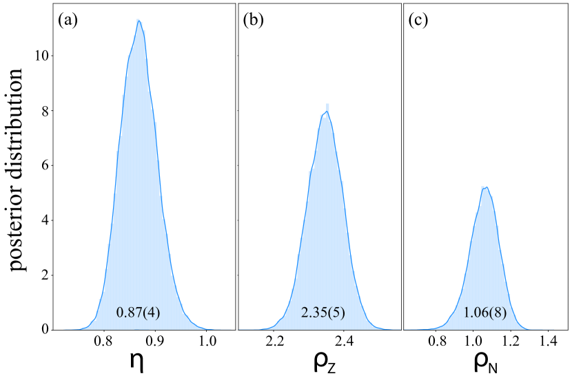
Figure 4: Posterior distributions of the GP parameters, with the posterior mean and standard deviation listed.

In Fig. 4 we show the posterior distributions of the GP parameters in the case of the DD-PC1 model. It is seen that all three parameters are well determined with relatively narrow bell-shaped densities. The general scale of the statistical fluctuations is given by $\eta$ at 0.87 MeV. The parameters $\rho_{Z}$ and $\rho_{N}$ give the range of the correlation effects along the $Z$ and $N$ directions, respectively, with precisely $68\%$ concentrated within the neighborhood of size $2\rho$ and $95\%$ within that of size $4\rho$. Here we can assert that about $90\%$ of the correlation effects are located in the region $Z\pm 4$, $N\pm 2$. We recall that the $\sigma$ parameter in (3) scaling the experimental errors was set to 0.0235 MeV, which is the average of the error bars reported.

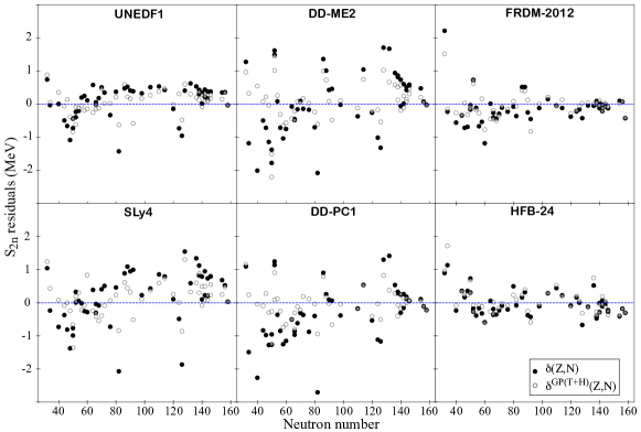
Figure 5: Residuals of $S_{2n}(Z,N)$ for the six global mass models with respect to the testing dataset (AME2016-AME2003): $\delta(Z,N)$ (dots) and the GP emulator $\delta^{\mathrm{GP}}(Z,N)$ (circles).

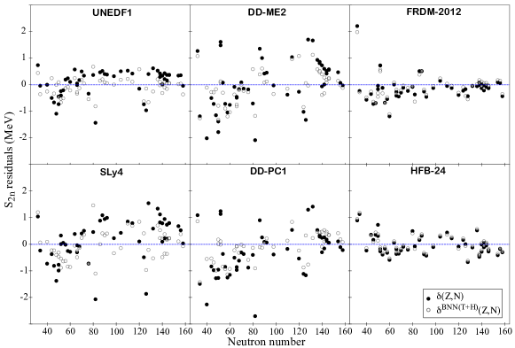
Figure 6: Residuals of $S_{2n}(Z,N)$ for the six global mass models with respect to the testing dataset (AME2016-AME2003): $\delta(Z,N)$ (dots) and the BNN emulator $\delta^{\mathrm{BNN}}(Z,N)$ (circles).

V Results

V.1 Training set: AME2003, testing set: AME2016

To test the predictive power of theoretical models and performance of statistical models, we first carried out calculations involving the training datasets AME2003 and AME2003-H and the testing dataset AME2016-AME2003. The results are presented in Figs. 5 and 6 and Table 1. It is to be noted that AME2016 contains data on remeasured masses since the AME2003 compilation. In some cases, the differences between old and new data can be significant (up to 30% difference), especially for light nuclei. Given the overall consensus that the AME2016 values are more accurate, the points in question, namely ${}^{1}0$He, ²⁴O, ³⁴Mg and ⁵²Ca, are removed from the AME2003 training dataset. Of course this correction is applied only to the emulator trained on AME2003, solely for the purpose of providing meaningful evaluations, and all other training sets incorporate the most recent measurement available to-date.

Figures 5 and Fig. 6 show the residuals of six representative nuclear mass models as a function of the neutron number before and after statistical corrections with GP(T+H) and BNN(T+H) respectively. In both GP and BNN, one observes that nearly every white circle, corresponding to a prediction error of our emulator for a given nucleus, is closer to the data than its corresponding black dot, representing a global mass model prediction error without GP or BNN. This indicates that both GP and BNN corrections improve the predictions systematically. Additionally, several local trends of the residuals are visibly attenuated, and the distributions of the corrected residuals are closer to having zero means and to being independent Gaussian. We observe that the improvement in performance for our statistical correction is strongest for the relativistic DFT models (DD-ME2 and DD-PC1), and weakest for the more phenomenological models FRDM-2012 and HFB-24. This is not surprising, as we expect the residuals of more microscopic models to exhibit appreciable structure, whereas there is little hope to improve much the phenomenological models which are fitted closely to the data.

Table 1 lists the rms values of residuals obtained in various mass models using four different variants, and the two GP and BNN statistical approaches, for emulators $\delta^{\mathrm{em}}(Z,N)$. Both GP and BNN reduce the rms residuals of $S_{2n}$ noticeably, with GP having a significantly better performance. Both GP and BNN perform best on the relativistic DFT models (around 50% rms reduction), second on the Skyrme-DFT models (around 30% rms reduction), and then on the more phenomenological models FRDM-2012 and HFB-24 which are already very well optimized to nuclear masses, as we noted (around 10% rms reduction); this is consistent with the corresponding levels of structure seen in Fig. 3. The increase in the predictive power of DFT-based models aided by the statistical treatment of residuals is significant: the rms deviation from experiment in the T+H variant shows that the carefully optimized Skyrme-DFT models, such as UNEDF0, UNEDF1, and SV-min, provide results of a similar quality than more phenomenological models. Overall, for the testing dataset AME2016-2003, the rms deviation from experimental $S_{2n}$ values is 400-500 keV in the GP(T+H) variant for all theoretical models employed in this study, which suggests that our statistical methods capture most of the residual structure. At this point, however, we shall re-emphasize the importance of carrying out the full UQ analysis to assess the quality of a model: the predicted mean value is certainly not the whole story.

Table 1: Root mean square values of $\delta(Z,N)$, $\delta^{\mathrm{BNN}}(Z,N)$, and $\delta^{\mathrm{GP}}(Z,N)$ (in MeV) for various nuclear models with respect to the testing dataset consisting of the AME2016-AME2003 $S_{2n}$ values. The training AME2003 and AME2003-H datasets were used to compute the emulators $\delta^{\mathrm{BNN}}(Z,N)$ and $\delta^{\mathrm{GP}}(Z,N)$. The two numbers listed under the model’s name in the first column are the uncorrected $\delta_{\mathrm{rms}}$ model values with respect to AME2003 and AME2003-H datasets, respectively. The rms residuals corrected by a statistical model are shown in the remaining columns. For each model, GP results $\delta^{\mathrm{GP}}_{\mathrm{rms}}$ are given in the upper row and the BNN results $\delta^{\mathrm{BNN}}_{\mathrm{rms}}$ are listed in the lower row. The numbers in parathenses indicate the improvement in percent. The four statistical variants are listed: Std is the standard treatment with the AME2003 training dataset; T indicates results involving the non-linear transformation $\tilde{x_{i}}=(d_{N}(x_{i}),p(x_{i}))$; H is based on the reduced dataset AME2003-H pertaining to heavy nuclei with $Z\geq 20$.

model	Std	T	H	T+H
SkM* 1.25/1.01	0.96(23)	0.96(23)	0.49(52)	0.49(52)
	0.99(20)	0.81(35)	0.73(28)	0.53(47)
SLy4 0.95/0.80	0.82(13)	0.82(13)	0.52(35)	0.52(35)
	0.91(3)	0.82(14)	0.71(11)	0.56(30)
SkP 0.84/0.62	0.75(11)	0.75(11)	0.38(39)	0.38(39)
	0.76(9)	0.74(12)	0.59(5)	0.45(27)
SV-min 0.78/0.49	0.70(10)	0.70(10)	0.32(34)	0.33(34)
	0.72(8)	1.35(-73)	0.50(-1)	0.43(12)
UNEDF0 0.78/0.54	0.73(6)	0.73(6)	0.34(37)	0.34(37)
	0.87(-12)	0.73(7)	0.55(0)	0.46(16)
UNEDF1 0.66/0.49	0.61(8)	0.61(8)	0.34(30)	0.34(30)
	0.79(-20)	0.74(-12)	0.53(-10)	0.32(33)
NL3* 1.19/0.86	0.84(29)	0.84(29)	0.46(47)	0.45(47)
	1.10(7)	0.90(24)	0.83(4)	0.69(20)
DD-ME$\bm{\delta}$ 1.13/0.96	0.73(35)	0.74(35)	0.55(42)	0.55(42)
	1.08(4)	0.91(19)	0.89(7)	0.75(22)
DD-ME2 1.04/0.95	0.71(32)	0.71(31)	0.63(34)	0.62(34)
	1.00(4)	1.32(-27)	0.90(5)	0.61(36)
DD-PC1 1.10/0.91	0.79(28)	0.79(28)	0.46(50)	0.46(50)
	1.00(9)	1.33(-22)	0.85(7)	0.54(41)
FRDM-2012 0.63/0.49	0.57(9)	0.57(9)	0.36(25)	0.36(26)
	0.61(4)	0.72(-15)	0.48(2)	0.45(7)
HFB-24 0.40/0.37	0.40(-1)	0.40(-1)	0.40(-8)	0.40(-8)
	0.59(-48)	0.44(-10)	0.37(1)	0.35(6)

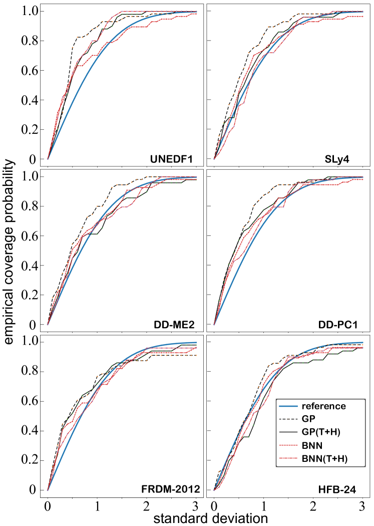
Figure 7: Empirical coverage probability for the six models used in our study as functions of multiples of the standard deviation (s.d.). The reference curve corresponds to the Gaussian quantiles, i.e., the probability that new testing data fall into the corresponding CI according to the domain. That is, at 1 s.d, the reference curve is 0.68 (and 68 % of the testing data should fall into the CI); at 2 s.d. it is 0.95, and so on.

Figure 7 shows what is known as empirical coverage probability (ECP), which is the simple and intuitive metric for assessing the quality of a statistical model’s quantification of uncertainty (see Sec. III.3 and Refs. Gneiting and Raftery (2007); Gneiting et al. (2007)). In Fig. 7, for every model, the reference curve shows the fraction of predictions which should theoretically fall in a CI centered around the posterior mean prediction, for any given interval width (measured in posterior standard deviations under normal distribution). In that figure, every one of the other four curves shows the actual fraction of the residuals of the testing data that belong to each such CI for BNN and GP, respectively, with and without the T+H variant. A prediction point above the reference curve represents a posterior CI which is too wide because it covers too many points. Thus, it can be considered as a prediction which is too conservative (or too pessimistic). As we mentioned before, while not necessarily dishonest, this could be considered potentially wasteful. A point below the reference curve represent a CI which is too narrow, which is too liberal (or too optimistic). This should be considered dishonest, since it is claiming a level of assurance which is higher than it should be. Values for the empirical proportions, which are close to the nominal values of the reference curve are desirable. In fact, to guard against the risk of giving predictions which are slightly too optimistic, one is better off hoping for ECPs which are slightly conservative. At the level of discussing uncertainty on the uncertainty, aiming for slightly conservative CIs increases the chances that one’s predictions are sufficiently honest and not very wasteful.

This objective is, in fact, quite what we observe in Fig. 7. Regardless of the nuclear physics model or statistical method considered, the distribution of the testing data matches closely the CIs predicted. The predicted CIs are slightly conservative for most models - the empirical curve is slightly above the reference curve - with the exception of HFB-24. Indeed, since HFB-24 matches closely the training data due to its fairly phenomenological nature, the statistical uncertainty estimated is very low and does not represent accurately the uncertainty on points which have not been used in the fit. Overall, the shape of the ECP curves clearly validates the honesty of our approach, and supports using our corrected predictions for future measurements with Bayesian CIs.

V.2 Training set AME2016-H, testing set JYFLTRAP data

Table 2: Similar as in Table 1 except for the rms values of $\delta(Z,N)$, $\delta^{\mathrm{BNN}}(Z,N)$, and $\delta^{\mathrm{GP}}(Z,N)$ (in MeV) for various nuclear models with respect to the testing dataset consisting of the four JYFLTRAP $S_{2n}$ values. The second column shows the uncorrected rms value $\delta_{\mathrm{rms}}$. For each model, the training datasets AME2003-H (third column) and AME2016-H (fourth column) were used to compute $\delta^{\mathrm{GP}}_{\mathrm{rms}}$ (upper row) and $\delta^{\mathrm{BNN}}_{\mathrm{rms}}$ (lower row) using the T+H variant of statistical calculations.

model	$\delta_{\rm rms}$	2003-H	2016-H
SkM*	0.91	0.40(56)	0.31(66)
		0.24(74)	0.25(72)
SLy4	0.27	0.09(65)	0.09(67)
		0.42(-57)	0.28(-4)
SkP	0.19	0.16(14)	0.14(26)
		0.35(-85)	0.36(-92)
SV-min	0.14	0.11(18)	0.10(29)
		0.17(-20)	0.26(-86)
UNEDF0	0.11	0.11(-3)	0.11(1)
		0.33(-199)	0.22(-97)
UNEDF1	0.26	0.17(36)	0.14(48)
		0.09(64)	0.13(50)
NL3*	0.32	0.19(39)	0.22(32)
		0.17(47)	0.18(43)
DD-ME$\bm{\delta}$	0.16	0.08(50)	0.09(46)
		0.18(-14)	0.28(-4)
DD-ME2	0.30	0.12(58)	0.13(55)
		0.28(8)	0.29(2)
DD-PC1	0.28	0.17(41)	0.13(52)
		0.25(12)	0.27(5)
FRDM-2012	0.13	0.10(20)	0.09(26)
		0.05(60)	0.05(58)
HFB-24	0.13	0.12(2)	0.11(12)
		0.07(43)	0.10(25)

We now investigate the impact of the extended training dataset on an extrapolation outcome. To this end, we compare predictions based on AME2003-H and AME2016-H training datasets on the recently measured masses at JYFLTRAP. The results are summarized in Table 2. The model rms residuals $\delta_{\mathrm{rms}}$ follow the trend discussed in Sec. V.1. Namely, the models FRDM-2012 and HFB-24 make predictions very close to the data ($\delta_{\mathrm{rms}}=0.13$ MeV) as well as the recently developed EDFs UNEDF0, SV-min, and DD-ME $\delta$ ($\delta_{\mathrm{rms}}=0.11-0.16$ MeV). Overall, the GP approach reduces the rms residuals significantly. This is consistent with Fig. 2, which shows that the local surface of $\delta(Z,N)$ is fairly smooth in the region of JYFLTRAP data ($Z\sim 62,N\sim 100$). On other other hand, the BNN method is not effective: for SLy4, SkP, SV-min, UNEDF0, and DD-ME$\delta$ one can see a deterioration of results. This is indicative of a sensitivity of BNN to long-scale correlations that can result in numerical instabilities discussed in Sec. V.4.

The difference between results based on AME2003-H and AME2016-H training datasets is insignificant. Overall, we find that the more recent mass measurements contained in the AME2016-AME2003 dataset do not impose constraints that are strong enough to modify predictions in the a smooth region of the mass surface. A similar conclusion was reached in Ref. McDonnell et al. (2015) in the context of Bayesian model studies.

V.3 Extrapolations

As a follow-up to the two previous exercises we now train the statistical emulators on the full set of available data for heavy nuclei, i.e., AME2016-H and JYFLTRAP. The simulations described in Secs. V.1 and V.2, on the testing sets, serve as a validation that our methodology is sound from a UQ perspective and is capable of providing accurate predictions. Perhaps the most important element of our UQ is the reliability of our CIs, which was assessed in Sec. V.1 by the analysis of ECPs at all credibility levels. Since our UQ is only slightly conservative, it essentially preserves the methodology’s full predictive (extrapolation) power.

The question at hand is how far can one extrapolate to provide reliable predictions. One can adopt several approaches to answer this question according to the particular problem of interest, but the general foundation is that we should trust the obtained Bayesian CIs since they have been validated by our analysis of the ECPs on points outside the training domain (see Sec. V.1 and Fig. 7), with the limitation that the testing points were relatively close to the training domain.

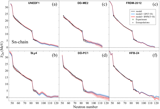
Figure 8: Extrapolations of $S_{2n}$ for the even-even Sn chain calculated with the six global mass models with statistical correction $\delta^{\mathrm{em}}$ and one-sigma CIs obtained with GP(T+H) and BNN(T+H). Experimental (circles) and extrapolated (asterisks) values from AME2016 Wang et al. (2017) are marked.

Figure 8 shows the extrapolative predictions of GP and BNN for the six representative global mass models for the Sn chain. As discussed in Sec. II, the DFT calculations are terminated when $\lambda_{n}$ becomes positive. This provides a rigid cutoff on mass model predictions. The Bayesian models estimate both corrections $\delta^{\mathrm{em}}$ to mass model results as well as error bars expressed in terms of CIs. Since the GP model is fairly local, by construction it goes faithfully through experimental points and the corresponding value $\delta^{\mathrm{em}}$ vanishes shortly outside the experimental data range. This is not the case for the BNN approach, which is more sensitive to long-range trends. Still, GP and BNN results are fairly close, and their CIs overlap in most cases. The empirical values for ^136,138Sn obtained from extrapolations in Ref. Wang et al. (2017) are very well reproduced by both GP and BNN. The size of CIs is consistent with the pattern of ECPs in Fig. 7: the largest error bars are obtained for the relativistic DFT models (DD-ME2 and DD-PC1), and smallest for the more phenomenological models FRDM-2012 and HFB-24. The error bars increase steadily when going away from the experimentally known region.

The small CIs predicted for HFB-24 require a comment. As seen in Fig. 7, HFB-24 is the only model to slightly underestimate the uncertainties. In fact, HFB-24 has been fitted to the AME2012 dataset that matches closely the training dataset AME2003. This causes our emulator to be blind to the actual underlying uncertainty of HFB-24 outside its training domain and results both in an underevaluation of the uncertainties on AME2016-AME2003 visible in Fig. 7 and the illusion of smaller CIs on the extrapolations in Fig. 8. In the context of a discussion about UQ, one would be tempted to reject the use of HFB-24 in the context of the statistical analysis because it is not honest enough; to avoid doing so, one would want to incorporate an additional error term in the statistical model based on HFB-24, one which takes into account additional uncertainty when making predictions outside of the training domain. In general, for highly parameterized models that are very well fitted to experimental data, the statistical approach described in this paper is not going to improve much as the random term in Eq. (3) becomes comparable with the function $f$ describing systematic patterns of model residuals.

A direct inspection of the CIs in Fig. 8 shows the most conservative estimate of the location of the $2n$-dripline ($S_{2n}=0$) around $N=104$, as in BNN with SLy4 and DD-PC1. If one were to stick to the GP approach, one would place the $2n$-dripline around $N=120$. The flatness of the posterior mean curves for our statistical emulators for large neutron numbers implies that any quantified determination of the location of the $2n$ dripline will be rather highly sensitive to the size of that uncertainty (e.g., the posterior standard deviation). This flatness also implies that one should decide whether the one-sigma intervals are at a sufficiently high level of credibility. One-sigma error bar implies 68% chance that the true value of predicted quantity falls within estimated error bars. One might consider using two-sigma intervals, corresponding to a CI of roughly 95%. The flatness of the prediction curve would then significantly decrease the drip line location.

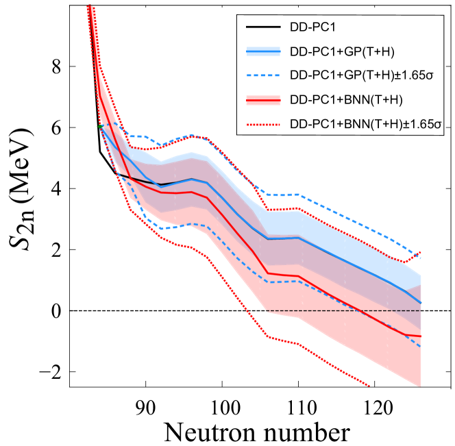
Figure 9: Extrapolations of $S_{2n}$ for the even-even Sn chain calculated with DD-PC1 with statistical GP(T+H) and BNN(T+H) approaches. One-sigma and 1.65-sigma CIs are marked.

If the objective is to predict the location of $2n$ dripline for an isotopic chain, a one-sided CI may be more appropriate. For fixed $Z$, the task is to find the largest value $N^{*}$such that the Bayesian posterior probability that the dripline is below $N^{*}$ exceeds $1-\alpha$. The answer to this question would then be roughly equivalent to finding the value $N^{*}$ such that the endpoint of its one-sided $1.65$-sigma CI barely touches the $S_{2n}=0$ line. This procures a predictive advantage over simply reading measurements off of two-sided CIs, since, by extending a one-sided interval to the level 1.65-sigma, one reaches a credibility of $95\%$, i.e., odds of about 20 to 1 for being right about a dripline. Figure 9 illustrates this approach for the dripline of Sn isotopes predicted with DD-PC1 using the statistical GP(T+H) and BNN(T+H) methods. In this case, the DD-PC1 model and DD-PC1+GP(T+H) predict the $2n$ dripline at $N^{*}=126$ for its posterior mean value (with $N^{*}=122$ and 118 at the 1-sigma and 1.65-sigma levels, respectively) while the DD-PC1+BNN(T+H) model gives a prediction of $N^{*}=118$ ($N^{*}=102$ and 104 at 1-sigma and 1.65-sigma level, respectively). This discussion demonstrates the naïvety of the absolute declarations, such as: “DD-PC1 predicts the $2n$ dripline at $N=126$.” Note that Figure 9 also contains the right-hand limit of the 1-sigma and 1.65-sigma CIs, but this information is not needed to interpret a lower credibility limit on a dripline. Again, as stated, to be safe, we recommend using the neutron-number location where the 1.65-sigma CI crosses the zero-$S_{2n}$ level as a lower limit for the dripline, since the probability of a model predicting the dripline being at this location or below is at least $95\%$.

V.4 Numerical considerations

Despite the apparent strong performance of BNN, it is necessary to provide some caveats based on our experience. Even when using up to 10⁷ Monte Carlo samples, the results are not completely stable throughout different simulation runs, in particular for extreme extrapolations. We illustrate this in Fig. 10 where we superpose the predictions and confidence intervals given by the DD-PC1 + BNN(T+H) model trained on AME2016+JYFLTRAP dataset for the Sn-chain, with two different MCMC runs with 100,000 samples (after 10,000-sample tuning) and 1,000,000 samples (after 100,000-sample tuning). Obviously one would expect the curves to match, but they can differ here significantly, even with a high number of iterations.

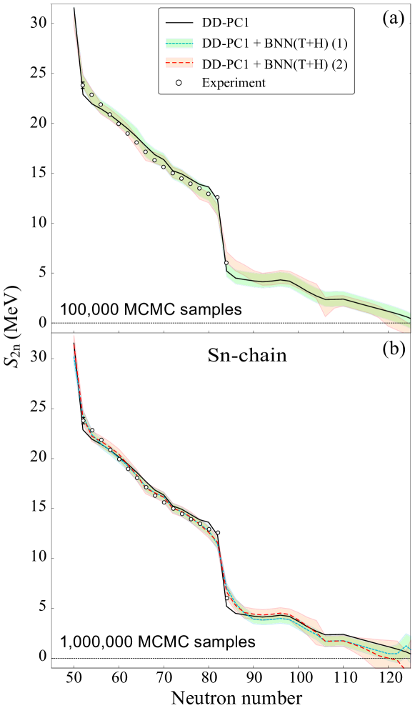
Figure 10: Predictions and confidence intervals given by DD-PC1+BNN(T+H) for the Sn chain for (a) two MCMC runs using 100,000 samples (after 10,000-sample tuning) and (b) two MCMC runs using 1,000,000 samples (after 100,000-sample tuning). The curve (1) in the top panel corresponds to the BNN(T+H) curve of Fig. 8(d).

Strong evidence exists to argue that the numerical instabilities inherent to BNN are related to the large number of parameters used. Examples of numerical errors on real data problems, associated with convergence difficulties, can be found in Ch. 4.4 of Ref. Neal (1996). A systematic investigation of discrepancies between several BNN runs is difficult to evaluate for our problem, because it would require extensive computations. However, investigating the convergence of BNN can be done at a relatively low cost. This leads to the results shown in Fig. 11.

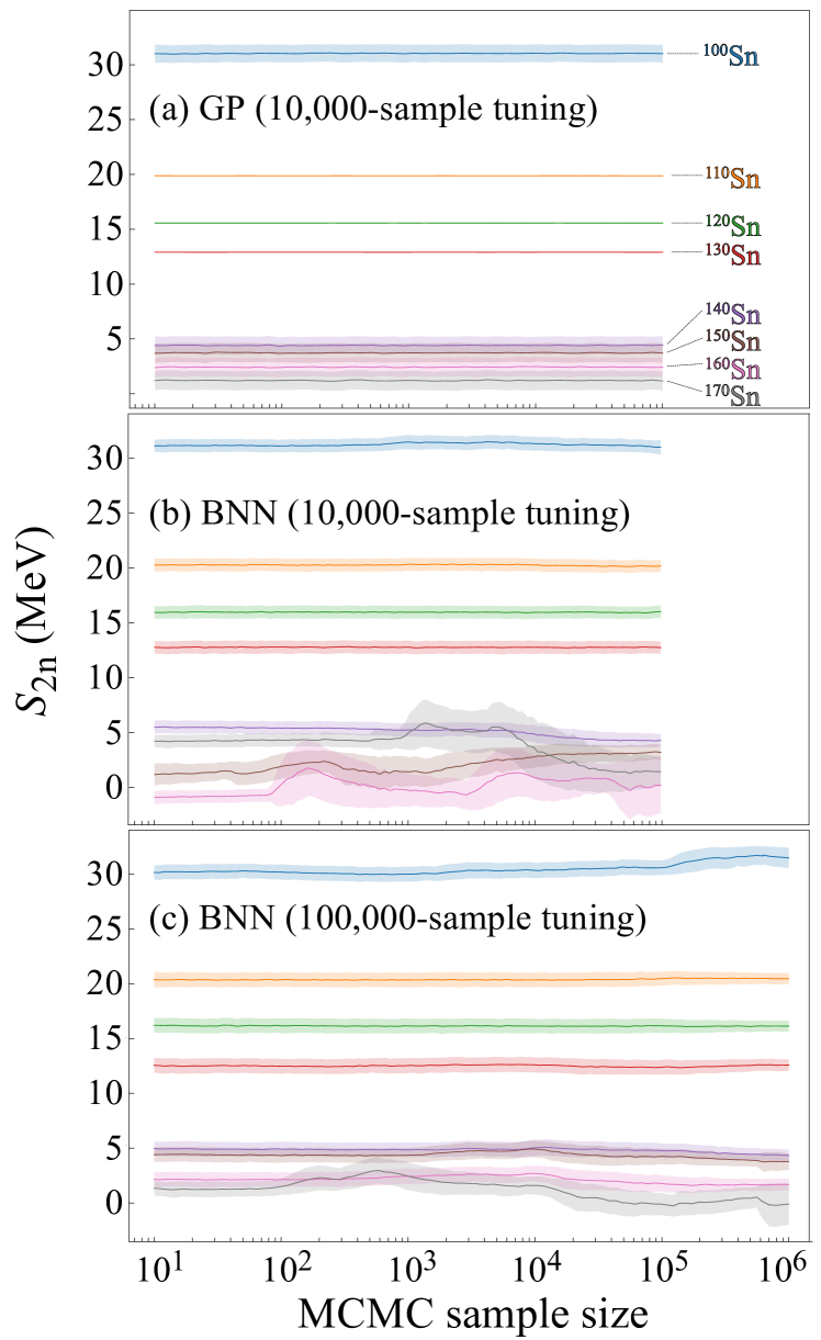
Figure 11: Posterior sample mean and standard deviation of $S_{2n}$ for several Sn isotopes predicted in DD-PC1. The statistical calculations were carried out with GP(T+H) and BNN(T+H) methods trained on the AME2016+JYFLTRAP dataset. The results are shown as a function of the number of MCMC samples. The number of samples used initially for tuning was 10,000 (panels a and b) and 100,000 (panel c).

One can see that after using 10,000 samples for tuning, the posterior predictions and uncertainties of the GP emulator are clearly in a stationary regime, but it takes about 100,000 samples for BNN to reach the same level. In general, convergence of MCMC estimators is governed by the Central Limit Theorem (CLT) according to which the convergence rate behaves as $\frac{C}{\sqrt{n}}$, where the constant $C$ corresponds to the largest eigenvalue of the autocovariance matrix of the Markov chain Jones (2004). For models with many parameters such as BNN, correlation between samples cannot be avoided with the traditional algorithms of Metropolis(-Hastings) or Gibbs. Convergence can be improved by so-called ’variance reduction techniques’ which aim at decreasing the constant $C$. A number of Bayesian nuclear mass studies Utama et al. (2016a, b); Utama and Piekarewicz (2017, 2018); Niu and Liang (2018) has relied on the “Flexible Bayesian Modeling” software Neal (1996), which is based on a combination of Gibbs and Metropolis algorithms, which can improve numerical convergence. Other suggestions in Ref. Neal (1996) to improve convergence include changing priors to non-Gaussian stable distributions or using simulated annealing. Modern approaches favor the use of more advanced MCMC techniques relying on an energy density known as Hamiltonian Monte Carlo methods such as NUTS Hoffman and Gelman (2014); Levy et al. (2018), which explore the space more wisely and converge in less steps, however, at some significant increased cost in terms of evaluation time. The underlying idea is that convergence of Markov chains on bounded spaces occurs at the exponential rate $\rho^{n}$ where $0<\rho\leq 1$ is the largest eigenvalue of the transition matrix of the parameters. This exponential convergence can only be achieved when the proposal distribution matches the actual distribution, which requires an adequate exploration of the space Mergersen and Tweedie (1996). In our simulations, however, NUTS and Metropolis sampler achieved similar convergence for comparable computation time although fine tuning could improve NUTS. Because of the CLT limitation, our best option to improve the convergence of BNN would be to increase the number of simulations by two orders of magnitude, which would require unreasonable levels of computational resources, making the method impractical.

All the numerical issues encountered in BNN are essentially absent in the case of GP, which has a very small number of parameters (three) in comparison to BNN (over one hundred). This numerical stability is an additional argument, beyond parsimony, in favor of GP over BNN. We must mention that the evaluation of the prediction samples from the model parameters requires sampling from a multivariate Gaussian kernel, which can take significantly more time than in the case of BNN, but far less than the factor of 100 which would be needed to improve BNN’s stability.

VI Conclusions

There is a vast amount of information contained in the residuals of theoretical models’ predictions. To improve the fidelity of theoretical predictions, especially in the context of extrapolations, one can utilize Bayesian machine learning techniques such as GP or BNN, which can quantify patterns of deviations between theory and experiment. Stochastic simulations based on MCMC sampling provide statistical corrections to average prediction values, and offer full uncertainty quantification on predictions through credibility intervals.

In this study, we investigated patterns of $2n$ separation energies of even-even nuclei calculated by several global mass models. We proceeded in three steps. First, we trained our statistical models on large learning datasets of experimentally known $S_{2n}$ values. We then made extrapolative predictions for the testing datasets consisting of more recently measured separation energies, as a way to validate the statistical method’s predictive performance. Having thus established and validated a statistical methodology, including a determination of its parameters, we then carried out predictions for unknown data.

We see that although both GP or BNN reduce the rms deviation from experiment significantly, GP has a better and more stable performance (see Tables 1 and 2). Both GP and BNN perform best on the relativistic DFT models, second on the Skyrme-DFT models, and then on the more phenomenological models FRDM-2012 and HFB-24, which are very well optimized to nuclear masses; this is consistent with the corresponding levels of structure that one could expect. The increase in the predictive power of DFT-based models aided by the statistical treatment is quite astonishing: the resulting rms deviation from experiment in the T+H variant (last column of Table 1) shows that the carefully optimized Skyrme-DFT models, such as UNEDF0, UNEDF1, and SV-min, provide results of a similar quality on the testing dataset as the more phenomenological models. Overall, for the testing dataset AME2016-2003, the rms deviation from experimental $S_{2n}$ values is in the 400-500 keV range in the GP T+H variant for the all theoretical models employed in this study.

We realized that, as the classical sigmoid activation function used in BNN has linear tails that do not vanish, it is poorly suited for a bounded extrapolation. This perhaps explains the better performance of GP, which builds the prediction locally with small bumps that can capture local trends. Indeed, our results indicate that the $S_{2n}$-residuals have an appreciable local structure around magic gaps, but no global structure. This is encouraging as it means that the models used are not missing any significant physics applicable on the whole nuclear domain. As a broader perspective, our results support using local Bayesian statistical models in combination with a well thought-out effect range, to reproduce the residuals trends, and to take advantage of models and other forms of physical intuition as part of building a Bayesian prior. At the same time, BNN should not be rejected as a poor extrapolation tool at all ranges. We emphasize that the statistical corrections and quantified uncertainties obtained by GP on extrapolations far from the range of the training data are negligible in practice, which is by design of the GP specification. It is also true that BNN extrapolations are possible beyond the range of influence of GP. However, in the absence of any supporting experimental data to test the performance of BNN far from the stability range, it is not possible to know whether the actual BNN corrections are of value in these long-range extrapolations. We contend that the main interest in Bayesian methods when applied to distant extrapolations lies in the UQ that their credibility intervals provide. As soon as a few data points in these distant ranges will become available, it will be possible to test BNN’s extrapolation performance using UQ as a framework for honest performance metrics.

Our Bayesian methodology is very robust in the sense of this type of performance framework. To this point, we showed how the ECP curves we obtain match the reference values very well, in a slightly conservative way in most cases, which is highly desirable to ensure UQ honesty without being wasteful (cf. discussion around Fig. 7).

The statistical approach to extrapolation of nuclear model results discussed in this paper can be very useful for assessing the impact of current and future experiments in the context of model developments. In the particular case studied in this work, the impact of the new data for unstable nuclei on the predictive power of theoretical models turned out to be minor. This is probably due the fact that the mass surface in the region of JYFLTRAP data is fairly smooth. This conclusion should not be generalized; rather, because the methodology provide a sound UQ, for instance, one should expect that any experiment planned near the boundary of a mass surface with limited smoothness should provide a significant advantage to extrapolations beyond that boundary. Other scenarios can also be imagined with similar positive impact of extrapolation from a small number of new data points near a boundary region. Such a scenario can be tested ahead of time, using synthetic data, with our methodology providing a full quantification of uncertainty based on the synthetic scenarii, to help experimenters decide if the experiment’s cost is worth the risk.

We also think that the new GP capability to evaluate residuals is expected to impact research in the domains where experiments are currently impossible, e.g., in studies of astrophysical nucleosynthesis processes.

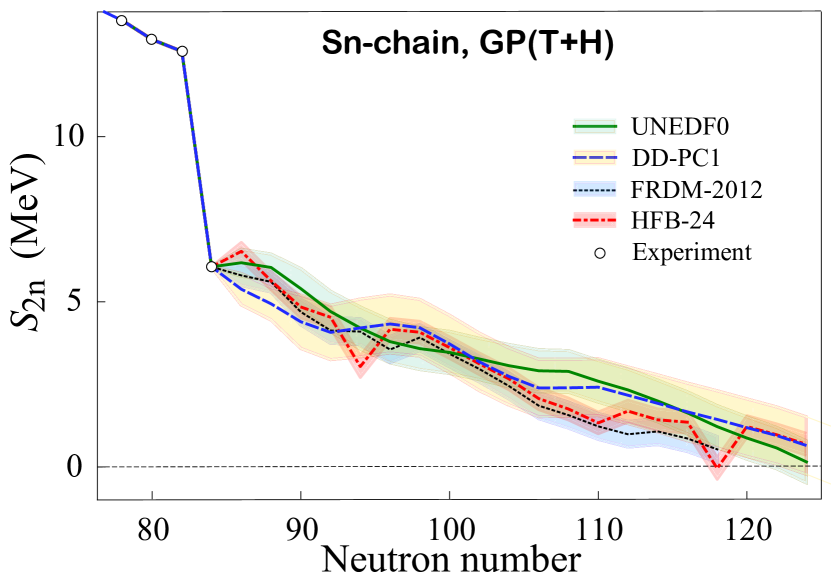
Figure 12: Extrapolations of $S_{2n}(Z,N)$ for the Sn chain corrected with GP(T+H) and one-sigma CIs, combined for four representative models. The different models are consistent overall once the statistical correction and uncertainty are taken into account.

Figure 12 illustrates this point nicely. It shows extrapolations of the $S_{2n}$-values for the even-even Sn isotopes for four global mass models aided by the statistical GP(T+H) approach. It is gratifying to see that all four models displayed provide internally consistent results, i.e., they agree with each other within the estimated CIs.

The example shown in Fig. 12 illustrates the limited value of assessing physics models solely based on their ability to fit experimental data. Clearly, mean values tell only part of the story. While HFB-24 and FRDM-2012 provide the superior reproduction of measured masses, their ability to extrapolate into the $r$-process region of neutron-rich nuclei is similar to that of DFT models based on well-optimized energy density functionals. Going further, we can strengthen our statements and decrease the sizes of uncertainty regions by combining the predictions’ CIs provided by GP and BNN for one mass model, and even of several mass models with Bayesian corrections (see Fig. 12). For a naïve look at this idea, one may consider the intersection of the various CIs.

When it comes to astrophysical applications, such as simulations of nucleosynthesis and models of the composition and structure of the neutron star crust, the methodology presented in this work can be directly applied to each observable of interest, such as one-neutron separation energies and $Q$-values for beta decay, alpha decay, and fission. The strategy, which we are going to adopt, is to provide Bayesian corrections and covariances for theoretical mass tables. Such information will allow the statistical determination of all mass differences, including precise statements about estimation precision, via a full quantification of their uncertainties.

There are other ways of further reducing theoretical uncertainty. For instance, it may be possible to decrease the residuals locally by fine-tuning model parameters to selected regional data. In this respect, measurements of masses of more exotic nuclei at rare isotope facilities will greatly add to the dataset that can be used in such analyses. Another way is to combine the predictions of several statistically corrected nuclear models, such as these shown in Fig. 12. Two Bayesian approaches can be used Hoeting et al. (1999); Wasserman (2000) in this context: model selection (the problem of using the data to select one model from a list of candidate models) and model averaging (estimating some quantity under each model and then averaging the estimates according to how likely each model is). In particular, an extrapolation based on a given model can run a significant misspecification risk, and this risk is typically never taken into account. Under Bayesian model selection/averaging, this risk can be quantified and taken into account, always resulting in a more honest UQ, and sometimes in more accurate extrapolation. These developments are left for a future study.

Finally, let us note that the information contained in the residuals shown, e.g., in Figs. 2 and 3, provides crucial guidance for the further developments of nuclear mass models. While statistical methods, which couple current nuclear models with available experimental data to maximize the use of existing information, can help providing more reliable predictions, they cannot be a substitute for the systematic development of high-fidelity theoretical models of the nucleus. The hope is that such models, guided by statistical methods, will allow us uncover nuclear structure features that may appear only far from stability.