A Swiss Army Infinitesimal Jackknife

Abstract

The error or variability of machine learning algorithms is often assessed by repeatedly re-fitting a model with different weighted versions of the observed data. The ubiquitous tools of cross-validation (CV) and the bootstrap are examples of this technique. These methods are powerful in large part due to their model agnosticism but can be slow to run on modern, large data sets due to the need to repeatedly re-fit the model. In this work, we use a linear approximation to the dependence of the fitting procedure on the weights, producing results that can be faster than repeated re-fitting by an order of magnitude. This linear approximation is sometimes known as the “infinitesimal jackknife” in the statistics literature, where it is mostly used as a theoretical tool to prove asymptotic results. We provide explicit finite-sample error bounds for the infinitesimal jackknife in terms of a small number of simple, verifiable assumptions. Our results apply whether the weights and data are stochastic or deterministic, and so can be used as a tool for proving the accuracy of the infinitesimal jackknife on a wide variety of problems. As a corollary, we state mild regularity conditions under which our approximation consistently estimates true leave-$k$-out cross-validation for any fixed $k$. These theoretical results, together with modern automatic differentiation software, support the application of the infinitesimal jackknife to a wide variety of practical problems in machine learning, providing a “Swiss Army infinitesimal jackknife.” We demonstrate the accuracy of our methods on a range of simulated and real datasets.

1 Introduction

Statistical machine learning methods are increasingly deployed in real-world problem domains where they are the basis of decisions affecting individuals’ employment, savings, health, and safety. Unavoidable randomness in data collection necessitates understanding how our estimates, and resulting decisions, might have differed had we observed different data. Both cross validation (CV) and the bootstrap attempt to diagnose this variation and are widely used in classical data analysis. But these methods are often prohibitively slow for modern, massive datasets, as they require running a learning algorithm on many slightly different datasets. In this work, we propose to replace these many runs with a single perturbative approximation. We show that the computation of this approximation is far cheaper than the classical methods, and we provide theoretical conditions that establish its accuracy.

Many data analyses proceed by minimizing a loss function of exchangeable data. Examples include empirical loss minimization and M-estimation based on product likelihoods. Since we typically do not know the true distribution generating the data, it is common to approximate the dependence of our estimator on the data via the dependence of the estimator on the empirical distribution. In particular, we often form a new, proxy dataset using random or deterministic modifications of the empirical distribution, such as randomly removing $k$ datapoints for leave-$k$-out CV. A proxy dataset obtained in this way can be represented as a weighting of the original data. From a set of such proxy datasets we can obtain estimates of uncertainty, including estimates of bias, variance, and prediction accuracy.

As data and models grow, the cost of repeatedly solving a large optimization problem for a number of different values of weights can become impractically large. Conversely, though, larger datasets often exhibit greater regularity; in particular, under fairly general conditions, limit laws based on independence imply that an optimum exhibits diminishing dependence on any fixed set of data points. We use this observation to derive a linear approximation to resampling that needs to be calculated only once, but which nonetheless captures the variability inherent in the repeated computations of classical CV. Our method is an instance of the infinitesimal jackknife (IJ), a general methodology that was historically a precursor to cross-validation and the bootstrap (Jaeckel, 1972; Efron, 1982). Part of our argument is that variants of the IJ should be reconsidered for modern large-scale applications because, for smooth optimization problems, the IJ can be calculated automatically with modern automatic differentiation tools (Baydin et al., 2017).

By using this linear approximation, we incur the cost of forming and inverting a matrix of second derivatives with size equal to the dimension of the parameter space, but we avoid the cost of repeatedly re-optimizing the objective. As we demonstrate empirically, this tradeoff can be extremely favorable in many problems of interest.

Our approach aims to provide a felicitous union of two schools of thought. In statistics, the IJ is typically used to prove normality or consistency of other estimators (Fernholz, 1983; Shao, 1993; Shao and Tu, 2012). However, the conditions that are required for these asymptotic analyses to hold are prohibitively restrictive for machine learning—specifically, they require objectives with bounded gradients. A number of recent papers in machine learning have provided related linear approximations for the special case of leave-one-out cross-validation (Koh and Liang, 2017; Rad and Maleki, 2018; Beirami et al., 2017), though their analyses lack the generality of the statistical perspective.

We combine these two approaches by modifying the proof of the Fréchet differentiability of M-estimators developed by Clarke (1983). Specifically, we adapt the proof away from the question of Fréchet differentiability within the class of all empirical distributions to the narrower problem of approximating the exact re-weighting on a particular dataset with a potentially restricted set of weights. This limitation of what we expect from the approximation is crucial; it allows us to bound the error in terms of a complexity measure of the set of derivatives of the observed objective function, providing a basis for non-asymptotic applications in large-scale machine learning, even for objectives with unbounded derivatives. Together with modern automatic differentiation tools, these results extend the use of the IJ to a wider range of practical problems. Thus, our “Swiss Army infinitesimal jackknife,” like the famous Swiss Army knife, is a single tool with many different functions.

2 Methods and Results

2.1 Problem definition

We consider the problem of estimating an unknown parameter $\theta\in\Omega_{\theta}\subseteq\mathbb{R}^{D}$, with a compact $\Omega_{\theta}$ and a dataset of size $N$. Our analysis will proceed entirely in terms of a fixed dataset, though we will be careful to make assumptions that will plausibly hold for all $N$ under suitably well-behaved random sampling. We define our estimate, $\hat{\theta}\in\Omega_{\theta}$, as the root of a weighted estimating equation. For each $n=1,\ldots,N$, let $g_{n}\left(\theta\right)$ be a function from $\Omega_{\theta}$ to $\mathbb{R}^{D}$. Let $w_{n}$ be a real number, and let $w$ be the vector collecting the $w_{n}$. Then $\hat{\theta}$ is defined as the quantity that satisfies

$$\hat{\theta}(w):= \quad\theta\textrm{ such that }\frac{1}{N}\sum_{n=1}^{N}w_{n}g_{n}\left(\theta\right)=0.$$ (1)

We will impose assumptions below that imply at least local uniqueness of $\hat{\theta}(w)$; see the discussion following 2 in Section 2.3.

As an example, consider a family of continuously differentiable loss functions $f\left(\cdot,\theta\right)$ parameterized by $\theta$ and evaluated at data points $x_{n},n=1,\ldots,N$. If we want to solve the optimization problem $\hat{\theta}=\underset{\theta\in\Omega_{\theta}}{\mathrm{argmin}}\frac{1}{N}\sum_{n=1}^{N}f\left(x_{n},\theta\right),$ then we take $g_{n}\left(\theta\right)=\partial f\left(x_{n},\theta\right)/\partial\theta$ and $w_{n}\equiv 1$. By keeping our notation general, we will be able to analyze a more general class of problems, such as multi-stage optimization (see Section 6). However, to aid intuition, we will sometimes refer to the $g_{n}\left(\theta\right)$ as “gradients” and their derivatives as “Hessians.”

When (LABEL:estimating_equation) is not degenerate (we articulate precise conditions below), $\hat{\theta}$ is a function of the weights through solving the estimating equation, and we write $\hat{\theta}(w)$ to emphasize this. We will focus on the case where we have solved (LABEL:estimating_equation) for the weight vector of all ones, $1_{w}:=\left(1,\ldots,1\right)$, which we denote $\hat{\theta}_{1}:=\hat{\theta}\left(1_{w}\right)$.

A re-sampling scheme can be specified by choosing a set $W\subseteq\mathbb{R}^{N}$ of weight vectors. For example, to approximate leave-$k$-out CV, one repeatedly computes $\hat{\theta}(w)$ where $w$ has $k$ randomly chosen zeros and all ones otherwise. Define $W_{k}$ as the set of every possible leave-$k$-out weight vector. Showing that our approximation is good for all leave-$k$-out analyses with probability one is equivalent to showing that the approximation is good for all $w\in W_{k}$.

In the case of the bootstrap, $W$ contains a fixed number $B$ of randomly chosen weight vectors, $w_{b}^{*}\stackrel{{\scriptstyle iid}}{{\sim}}\mathrm{Multinomial}\left(N,N^{-1}\right)$ for $b=1,\ldots,B$, so that $\sum_{n=1}^{N}w_{bn}^{*}=N$ for each $b$. Note that while $w_{n}$ or $w_{bn}^{*}$ are scalars, $w_{b}^{*}$ is a vector of length $N$. The distribution of $\hat{\theta}\left(w_{b}^{*}\right)-\hat{\theta}\left(1_{w}\right)$ is then used to estimate the sampling variation of $\hat{\theta}_{1}$. Define this set $W^{*}_{B}=\{w_{1}^{*},\ldots,w_{B}^{*}\}$. Note that $W^{*}_{B}$ is stochastic and is a subset of all weight vectors that sum to $N$.

In general, $W$ can be deterministic or stochastic, may contain integer or non-integer values, and may be determined independently of the data or jointly with it. As with the data, our results hold for a given $W$, but in a way that will allow natural high-probability extensions to stochastic $W$.

2.2 Linear approximation

The main problem we solve is the computational expense involved in evaluating $\hat{\theta}(w)$ for all the $w\in W$. Our contribution is to use only quantities calculated from $\hat{\theta}_{1}$ to approximate $\hat{\theta}(w)$ for all $w\in W$, without re-solving (LABEL:estimating_equation). Our approximation is based on the derivative $\frac{d\hat{\theta}(w)}{dw^{T}}$, whose existence depends on the derivatives of $g_{n}\left(\theta\right)$, which we assume to exist, and which we denote as $h_{n}\left(\theta\right):=\frac{\partial g_{n}\left(\theta\right)}{\partial\theta^{T}}$. We use this notation because $h_{n}\left(\theta\right)$ would be the Hessian of a term of the objective in the case of an optimization problem. We make the following definition for brevity.

Definition 1.

The fixed point equation and its derivative are given respectively by

$$G\left(\theta,w\right) :=\frac{1}{N}\sum_{n=1}^{N}w_{n}g_{n}\left(\theta\right)$$

$$H\left(\theta,w\right) :=\frac{1}{N}\sum_{n=1}^{N}w_{n}h_{n}\left(\theta\right).$$

Note that $G\left(\hat{\theta}(w),w\right)=0$ because $\hat{\theta}(w)$ solves (LABEL:estimating_equation) for $w$. We define $H_{1}:=H\left(\hat{\theta}_{1},1_{w}\right)$ and define the weight difference as $\Delta w=w-1_{w}\in\mathbb{R}^{N}$. When $H_{1}$ is invertible, one can use the implicit function theorem and the chain rule to show that the derivative of $\hat{\theta}(w)$ with respect to $w$ is given by

$$\frac{d\hat{\theta}(w)}{dw^{T}}\rvert_{1_{w}}\Delta w =-H_{1}^{-1}\frac{1}{N}\sum_{n=1}^{N}g_{n}\left(\hat{\theta}_{1}\right)\Delta w$$

$$=-H_{1}^{-1}G\left(\hat{\theta}_{1},\Delta w\right).$$

This derivative allows us to form a first-order approximation to $\hat{\theta}(w)$ at $\hat{\theta}_{1}$.

Definition 2.

Our linear approximation to $\hat{\theta}(w)$ is given by

$$\hat{\theta}_{\textrm{IJ}}\left(w\right) :=\hat{\theta}_{1}-H_{1}^{-1}G\left(\hat{\theta}_{1},\Delta w\right).$$

We use the subscript “IJ” for “infinitesimal jackknife,” which is the name for this estimate in the statistics literature (Jaeckel, 1972; Shao, 1993). Because $\hat{\theta}_{\textrm{IJ}}$ depends only on $\hat{\theta}_{1}$ and $\Delta w$, and not on solutions at any other values of $w$, there is no need to re-solve (LABEL:estimating_equation). Instead, to calculate $\hat{\theta}_{\textrm{IJ}}$ one must solve a linear system involving $H_{1}$. Recalling that $\theta$ is $D$-dimensional, the calculation of $H_{1}^{-1}$ (or a factorization that supports efficient solution of linear systems) can be $O\left(D^{3}\right)$. However, once $H_{1}^{-1}$ is calculated or $H_{1}$ is factorized, calculating our approximation $\hat{\theta}_{\textrm{IJ}}\left(w\right)$ for each new weight costs only as much as a single matrix-vector multiplication. Furthermore, $H_{1}$ often has a sparse structure allowing $H_{1}^{-1}$ to be calculated more efficiently than a worst-case scenario (see Section 6 for an example). In more high-dimensional examples with dense Hessian matrices, such as neural networks, one may need to turn to approximations such as stochastic second-order methods (Koh and Liang, 2017; Agarwal et al., 2017) and conjugate gradient (Wright and Nocedal, 1999). Indeed, even in relatively small or sparse problems, the vast bulk of the computation required to calculate $\hat{\theta}_{\textrm{IJ}}$ is in the computation of $H_{1}^{-1}$. We leave the important question of approximate calculation of $H_{1}^{-1}$ for future work.

2.3 Assumptions and results

We now state our key assumptions and results, which are sufficient conditions under which $\hat{\theta}_{\textrm{IJ}}(w)$ will be a good approximation to $\hat{\theta}(w)$. We defer most proofs to Appendix A. We use $\left\|\cdot\right\|_{op}$ to denote the matrix operator norm, $\left\|\cdot\right\|_{2}$ to denote the $L_{2}$ norm, and $\left\|\cdot\right\|_{1}$ to denote the $L_{1}$ norm. For quantities like $g$ and $h$, which have dimensions $N\times D$ and $N\times D\times D$ respectively, we apply the $L_{p}$ norm to the vectorized version of arrays. For example, $\frac{1}{\sqrt{N}}\left\|h\left(\theta\right)\right\|_{2}=\sqrt{\frac{1}{N}\sum_{n=1}^{N}\sum_{i=1}^{D}\sum_{j=1}^{D}\left[h_{n}\left(\theta\right)\right]_{ij}^{2}}$ which is the square root of a sample average over $n\in[N]$.

We state all assumptions and results for a fixed $N$, a given estimating equation vector $g\left(\theta\right)$, and a fixed class of weights $W$. Although our analysis proceeds with these quantities fixed, we are careful to make only assumptions that can plausibly hold for all $N$ and/or for randomly chosen $W$ under appropriate regularity conditions.

Assumption 1 (Smoothness).

For all $\theta\in\Omega_{\theta}$, each $g_{n}\left(\theta\right)$ is continuously differentiable in $\theta$.

The smoothness in 1 is necessary for a local approximation like 2 to have any hope of being useful.

Assumption 2 (Non-degeneracy).

For all $\theta\in\Omega_{\theta}$, $H\left(\theta,1_{w}\right)$ is non-singular, with $\sup_{\theta\in\Omega_{\theta}}\left\|H\left(\theta,1_{w}\right)^{-1}\right\|_{op}\leq C_{op}^{\text{\,}}<\infty$.

Without 2, the derivative in 2 would not exist. For an optimization problem, 2 amounts to assuming that the Hessian is strongly positive definite, and, in general, assures that the solution $\hat{\theta}_{1}$ is unique. Under our assumptions, we will show later that, additionally, $\hat{\theta}(w)$ is unique in a neighborhood of $\hat{\theta}_{1}$; see 6 of Appendix A. Furthermore, by fixing $C_{op}^{\text{\,}}$, if we want to apply 2 for $N\rightarrow\infty$, we will require that $H_{1}$ remains strongly positive definite.

Assumption 3 (Bounded averages).

There exist finite constants $C_{g}$ and $C_{h}$ such that $\sup_{\theta\in\Omega_{\theta}}\frac{1}{\sqrt{N}}\left\|g\left(\theta\right)\right\|_{2}\leq C_{g}<\infty\quad\textrm{and}\quad\sup_{\theta\in\Omega_{\theta}}\frac{1}{\sqrt{N}}\left\|h\left(\theta\right)\right\|_{2}\leq C_{h}<\infty$.

3 essentially states that the sample variances of the gradients and Hessians are uniformly bounded. Note that it does not require that these quantities are bounded term-wise. For example, we allow $\sup_{n}\left\|g_{n}\left(\theta\right)\right\|_{2}^{2}\underset{N\rightarrow\infty}{\longrightarrow}\infty$, as long as $\sup_{n}\frac{1}{N}\left\|g_{n}\left(\theta\right)\right\|^{2}_{2}$ remains bounded. This is a key advantage of the present work over many past applications of the IJ to M-estimation, which require $\sup_{n}\left\|g_{n}(\theta)\right\|_{2}^{2}$ to be uniformly bounded for all $N$ (Shao and Tu, 2012; Beirami et al., 2017).

In both machine learning and statistics, $\sup_{n}\left\|g_{n}(\theta)\right\|_{2}^{2}$ is rarely bounded, though $\frac{1}{N}\left\|g(\theta)\right\|_{2}^{2}$ often is. As a simple example, suppose that $\theta\in\mathbb{R}^{1}$, $x_{n}\sim\mathcal{N}(0,1)$, and $g_{n}=\theta-x_{n}$, as would arise from the squared error loss $f_{n}\left(x_{n},\theta\right)=\frac{1}{2}\left(\theta-x_{n}\right)^{2}$. Fix a $\theta$ and let $N\rightarrow\infty$. Then $\sup_{n}\left\|g_{n}(\theta)\right\|_{2}^{2}\rightarrow\infty$ because $\sup_{n}|x_{n}|\rightarrow\infty$, but $\frac{1}{N}\left\|g(\theta)\right\|_{2}^{2}\rightarrow\theta^{2}+1$ by the law of large numbers.

Assumption 4 (Local smoothness).

There exists a $\Delta_{\theta}>0$ and a finite constant $L_{h}$ such that, $\left\|\theta-\hat{\theta}_{1}\right\|_{2}\leq\Delta_{\theta}$ implies that $\frac{\left\|h\left(\theta\right)-h\left(\hat{\theta}_{1}\right)\right\|_{2}}{\sqrt{N}}\leq L_{h}\left\|\theta-\hat{\theta}_{1}\right\|_{2}$.

The constants defined in 4 are needed to calculate our error bounds explicitly.

Assumptions 1–4 are quite general and should be expected to hold for many reasonable problems, including holding uniformly asymptotically with high probability for many reasonable data-generating distributions, as the following lemma shows.

Lemma 1 (The assumptions hold under uniform convergence).

Let $\Omega_{\theta}$ be a compact set, and let $g_{n}\left(\theta\right)$ be twice continuously differentiable IID random functions for $n\in[N]$. (The function is random but $\theta$ is not—for example, $\mathbb{E}\left[g_{n}(\theta)\right]$ is still a function of $\theta$.) Define $r_{n}\left(\theta\right):=\frac{\partial^{2}g{}_{n}\left(\theta\right)}{\partial\theta\partial\theta}$, so $r_{n}\left(\theta\right)$ is a $D\times D\times D$ tensor.

Assume that we can exchange integration and differentiation, that $\mathbb{E}\left[h_{n}\left(\theta\right)\right]$ is non-singular for all $\theta\in\Omega_{\theta}$, and that all of $\mathbb{E}\left[\sup_{\theta\in\Omega_{\theta}}\left\|g_{n}\left(\theta\right)\right\|_{2}^{2}\right]$, $\mathbb{E}\left[\sup_{\theta\in\Omega_{\theta}}\left\|h_{n}\left(\theta\right)\right\|_{2}^{2}\right]$, and $\mathbb{E}\left[\sup_{\theta\in\Omega_{\theta}}\left\|r_{n}\left(\theta\right)\right\|_{2}^{2}\right]$ are finite.

Then $\lim_{N\rightarrow\infty}P\left(\textrm{Assumptions \ref{assu:paper_smoothness}--\ref{assu:paper_lipschitz} \ hold}\right)=1$.

1 follows from the uniform convergence results of Theorems 9.1 and 9.2 in Keener (2011). See Appendix A.4 for a detailed proof. A common example to which 1 would apply is where $x_{n}$ are well-behaved IID data and $g_{n}(\theta)=\gamma(x_{n},\theta)$ for an appropriately smooth estimating function $\gamma(\cdot,\theta)$. See Keener (2011, Chapter 9) for more details and examples, including applications to maximum likelihood estimators on unbounded domains.

Assumptions 1–4 apply to the estimating equation. We also require a boundedness condition for $W$.

Assumption 5 (Bounded weight averages).

The quantity $\frac{1}{\sqrt{N}}\left\|w\right\|_{2}$ is uniformly bounded for $w\in W$ by a finite constant $C_{w}$.

Our final requirement is considerably more restrictive, and contains the essence of whether or not $\hat{\theta}_{\textrm{IJ}}(w)$ will be a good approximation to $\hat{\theta}(w)$.

Condition 1 (Set complexity).

There exists a $\delta\geq 0$ and a corresponding set $W_{\delta}\subseteq W$ such that

$$\max_{w\in W_{\delta}}\sup_{\theta\in\Omega_{\theta}} \left\|\frac{1}{N}\sum_{n=1}^{N}\left(w_{n}-1\right)g_{n}\left(\theta\right)\right\|_{1}\leq\delta\quad\textrm{and}$$

$$\max_{w\in W_{\delta}}\sup_{\theta\in\Omega_{\theta}} \left\|\frac{1}{N}\sum_{n=1}^{N}\left(w_{n}-1\right)h_{n}\left(\theta\right)\right\|_{1}\leq\delta.$$

1 is central to establishing when the approximation $\hat{\theta}_{\textrm{IJ}}\left(w\right)$ is accurate. For a given $\delta$, $W_{\delta}$ will be the class of weight vectors for which $\hat{\theta}_{\textrm{IJ}}(w)$ is accurate to within order $\delta$. Trivially, $1_{w}\in W_{\delta}$ for $\delta=0$, so $W_{\delta}$ is always non-empty, even for arbitrarily small $\delta$. The trick will be to choose a small $\delta$ that still admits a large class $W_{\delta}$ of weight vectors. In Section 3 we will discuss 1 in more depth, but it will help to first state our main theorem.

Definition 3.

The following constants are given by quantities in Assumptions 1–5 .

$$C_{\textrm{IJ}} :=1+DC_{w}L_{h}C_{op}^{\text{\,}}$$

$$\Delta_{\delta} :=\min\left\{\Delta_{\theta}C_{op}^{-1},\frac{1}{2}C_{\textrm{IJ}}^{-1}C_{op}^{-1}\right\}.$$

Note that, although the parameter dimension $D$ occurs explicitly only once in 3, all of $C_{w}$, $C_{op}^{\text{\,}}$, and $L_{h}$ in general might also contain dimension dependence. Additionally, the bound $\delta$ in 1, a measure of the set complexity of the parameters, will typically depend on dimension. However, the particular place where the parameter dimension enters will depend on the problem and asymptotic regime, and our goal is to provide an adaptable toolkit for a wide variety of problems.

We are now ready to state our main result.

Theorem 1 (Error bound for the approximation).

Under Assumptions 1–5 and 1,

$$\delta\leq\Delta_{\delta}\Rightarrow\max_{w\in W_{\delta}}\left\|\hat{\theta}_{\textrm{IJ}}\left(w\right)-{\hat{\theta}(w)}\right\|_{2}\leq 2C_{op}^{2}C_{\textrm{IJ}}\delta^{2}.$$

We stress that 1 bounds only the difference between $\hat{\theta}_{\textrm{IJ}}(w)$ and $\hat{\theta}(w)$. 1 alone does not guarantee that $\hat{\theta}_{\textrm{IJ}}(w)$ converges to any hypothetical infinite population quantity. We see this as a strength, not a weakness. To begin with, convergence to an infinite population requires stronger assumptions. Contrast, for example, the Fréchet differentiability work of Clarke (1983), on which our work is based, with the stricter requirements in the proof of consistency in Shao (1993). Second, machine learning problems may not naturally admit a well-defined infinite population, and the dataset at hand may be of primary interest. Finally, by analyzing a particular sample rather than a hypothetical infinite population, we can bound the error in terms of the quantities $C_{\textrm{IJ}}$ and $\Delta_{\delta}$, which can actually be calculated from the data at hand.

Still, 1 is useful to prove asymptotic results about the difference $\left\|\hat{\theta}_{\textrm{IJ}}\left(w\right)-{\hat{\theta}(w)}\right\|_{2}$. As an illustration, we now show that the uniform consistency of leave-$k$-out CV follows from 1 by a straightforward application of Hölder’s inequality.

Corollary 1 (Consistency for leave-$k$-out CV).

Assume that Assumptions 1–5 hold uniformly for all $N$. Fix an integer $k$, and let

$$W_{k}:=\left\{w:w_{n}=0\textrm{ in }k\textrm{ entries and }1\textrm{ otherwise}\right\}.$$

Then, for all $N$, there exists a constant $C_{K}$ such that

$$\sup_{w\in W_{k}}\left\|\hat{\theta}_{\textrm{IJ}}\left(w\right)-{\hat{\theta}(w)}\right\|_{2} \leq C_{K}\frac{\left\|g\right\|_{\infty}^{2}}{N^{2}}$$

$$\leq C_{K}\frac{\max\left\{C_{g},C_{h}\right\}^{2}}{N}.$$

Proof.

For $w\in W_{k}$, $\frac{\left\|\Delta w\right\|_{2}}{\sqrt{N}}=\sqrt{\frac{K}{N}}.$ Define $C_{gh}:=\max\left\{C_{g},C_{h}\right\}$. By 3, $\left\|g\right\|_{2}/\sqrt{N}\leq C_{gh}$ and $\left\|h\right\|_{2}/\sqrt{N}\leq C_{gh}$ for all $N$. By Hölder’s inequality,

$$\sup_{w\in W}\sup_{\theta\in\Omega_{\theta}}\left\|\frac{1}{N}\sum_{n=1}^{N}\left(w_{n}-1\right)g_{n}\left(\theta\right)\right\|_{1}$$

$$\leq\sup_{w\in W}\left\|w-1_{w}\right\|_{1}\sup_{\theta\in\Omega_{\theta}}\frac{\left\|g\right\|_{\infty}}{N}=K\frac{\left\|g\right\|_{\infty}}{N}\leq K\frac{C_{gh}}{\sqrt{N}},$$

with a similar bound for $\left\|h\right\|_{2}$. Consequently, for $N$ large enough, 1 is satisfied with $W_{\delta}=W_{k}$ and either $\delta=K\frac{\left\|g\right\|_{\infty}}{N}$ or $\delta=K\frac{C_{gh}}{\sqrt{N}}$. The result then follows from 1. ∎

3 Examples

The moral of 1 is that, under Assumptions 1–5 and 1, $\left\|\hat{\theta}_{\textrm{IJ}}-{\hat{\theta}\left(w\right)}\right\|=O\left(\delta^{2}\right)$ for $w\in W_{\delta}$. That is, if we can make $\delta$ small enough, $W_{\delta}$ big enough, and still satisfy 1, then $\hat{\theta}_{\textrm{IJ}}\left(w\right)$ is a good approximation to $\hat{\theta}\left(w\right)$ for “most” $w$, where “most” is defined as the size of $W_{\delta}$. So it is worth taking a moment to develop some intuition for 1. We have already seen in Corollary 1 that $\hat{\theta}_{\textrm{IJ}}$ is, asymptotically, a good approximation for leave-$k$-out CV uniformly in $W$. We now discuss some additional cases: first, a worst-case example for which $\hat{\theta}_{\textrm{IJ}}$ is not expected to work, second the bootstrap, and finally we revisit leave-one-out cross validation in the context of these other two methods.

First, consider a pathological example. Let $W_{full}$ be the set of all weight vectors that sum to $N$. Let $n^{*}=\max_{n\in[N]}\left\|g_{n}\left(\hat{\theta}_{1}\right)\right\|_{1}$ be the index of the gradient term with the largest $L_{1}$ norm, and let $w_{n^{*}}=N$ and $w_{n}=0$ for $n\neq n^{*}$. Then

$$\sup_{\theta\in\Omega_{\theta}}\left\|\frac{1}{N}\sum_{n=1}^{N}\left(w_{n}-1\right)g_{n}\left(\theta\right)\right\|_{1}$$

$$\quad=\sup_{\theta\in\Omega_{\theta}}\left\|g_{n^{*}}\left(\theta\right)-\frac{1}{N}\sum_{n=1}^{N}g_{n}\left(\theta\right)\right\|_{1}\geq\left\|g_{n^{*}}\left(\hat{\theta}_{1}\right)\right\|_{1}.$$

(The last inequality uses the fact that $G\left(\hat{\theta}_{1},1_{w}\right)=0$.) In this case, unless the largest gradient, $\left\|g_{n^{*}}\left(\hat{\theta}_{1}\right)\right\|_{1}$, is small, 1 will not be satisfied for small $\delta$, and we would not expect $\hat{\theta}_{\textrm{IJ}}$ to be a good estimate for $\hat{\theta}\left(w\right)$ for all $w\in W_{full}$. The class $W_{full}$ is too expressive. In the language of 1, for some small fixed $\delta$, $W_{\delta}$ will be some very restricted subset of $W_{full}$ in most realistic situations.

Now, suppose that we are using $B$ bootstrap weights, $w_{b}^{*}\stackrel{{\scriptstyle iid}}{{\sim}}\mathrm{Multinomial}\left(N,N^{-1}\right)$ for $b=1,...,B$, and analyzing an optimization problem as defined in Section 2.1. For a given $w_{b}^{*}$, a dataset $x_{1}^{*},...,x_{N}^{*}$ formed by taking $w_{b,n}^{*}$ copies of datapoint $x_{n}$ is equivalent in distribution to $N$ IID samples with replacement from the empirical distribution on $\left(x_{1},...,x_{N}\right)$. In this notation, we then have

$$\frac{1}{N}\sum_{n=1}^{N}\left(w_{b}^{*}-1\right)g_{n}\left(\theta\right)=$$

$$\quad\frac{1}{N}\sum_{n=1}^{N}\frac{\partial f\left(\theta,x_{n}^{*}\right)}{\partial\theta}-\frac{1}{N}\sum_{n=1}^{N}\frac{\partial f\left(\theta,x_{n}\right)}{\partial\theta}.$$

In this case, 1 is a uniform bound on a centered empirical process of derivatives of the objective function. Note that estimating sample variances by applying the IJ with bootstrap weights is equivalent to the ordinary delta method based on an asymptotic normal approximation (Efron, 1982, Chapter 21). In order to provide an approximation to the bootstrap that retains benefits (such as the faster-than-normal convergence to the true sampling distribution described by Hall (2013)), one must consider higher-ordered Taylor expansions of $\hat{\theta}(w)$. We leave this for future work.

Finally, let us return to leave-one-out CV. In this case, $w_{n}-1$ is nonzero for exactly one entry. Again, we can choose to leave out the adversarially-chosen $n^{*}$ as in the first pathological example. However, unlike the pathological example, the leave-one-out CV weights are constrained to be closer to $1_{w}$—specifically, we set $w_{n^{*}}=0$, and let $w$ be one elsewhere. Then 1 requires $\sup_{\theta\in\Omega_{\theta}}\left\|\frac{1}{N}g_{n^{*}}\left(\theta\right)\right\|_{1}\leq\delta.$ In contrast to the pathological example, this supremum will get smaller as $N$ increases as long as $\left\|g_{n^{*}}\left(\theta\right)\right\|_{1}$ grows more slowly than $N$. For this reason, we expect leave-one-out (and, indeed, leave-$k$-out for fixed $k$) to be accurately approximated by $\hat{\theta}_{\textrm{IJ}}$ in many cases of interest, as stated in Corollary 1.

4 Related Work

Although the idea of forming a linear approximation to the re-weighting of an M-estimator has a long history, we nevertheless contribute in a number of ways. By limiting ourselves to approximating the exact reweighting on a particular dataset, we both loosen the strict requirements from the statistical literature and generalize the existing results from the machine learning literature.

The jackknife is often favored over the IJ in the statistics literature because of the former’s simple computational approach, as well as perceived difficulties in calculating the necessary derivatives when some of the parameters are implicitly defined via optimization (Shao and Tu, 2012, Chapter 2.1) (though exceptions exist; see, e.g., Wager et al. (2014)). The brute-force approach of the jackknife is, however, a liability in large-scale machine learning problems, which are generally extremely expensive to re-optimize. Furthermore, and critically, the complexity and tedium of calculating the necessary derivatives is entirely eliminated by modern automatic differentiation (Baydin et al., 2017; Maclaurin et al., 2015).

Our work is based on the proof of the Fréchet differentiability of M-estimators of Clarke (1983). In classical statistics, Fréchet differentiability is typically used to describe the asymptotic behavior of functionals of the empirical distribution in terms of a functional (Mises, 1947; Fernholz, 1983). Since Clarke (1983) was motivated by such asymptotic questions, he studied the Fréchet derivative evaluated at a continuous probability distribution for function classes that included delta functions. This focus led to the requirement of a bounded gradient. However, unbounded gradients are ubiquitous in both statistics and machine learning, and an essential contribution of the current paper is to remove the need for bounded gradients.

There exist proofs of the consistency of the (non-infinitesimal) jackknife that allow for unbounded gradients. For example, it is possible that the proofs of Reeds (1978), which require a smoothness assumption similar to our 4, could be adapted to the IJ. However, the results of Reeds (1978)—as well as those of Clarke (1983) and subsequent applications such as those of Shao and Tu (2012)—are asymptotic and applicable only to IID data. By providing finite sample results for a fixed dataset and weight set, we are able to provide a template for proving accuracy bounds for more generic probability distributions and re-weighting schemes.

A number of recent machine learning papers have derived approximate linear versions of leave-one-out estimators. Koh and Liang (2017) consider approximating the effect of leaving out one observation at a time to discover influential observations and construct adversarial examples, but provide little supporting theory. Beirami et al. (2017) provide rigorous proofs for an approximate leave-one-out CV estimator; however, their estimator requires computing a new inverse Hessian for each new weight at the cost of a considerable increase in computational complexity. Like the classical statistics literature, Beirami et al. (2017) assume that the gradients are bounded for all $N$. When $\left\|g\right\|_{\infty}^{2}$ in Corollary 1 is finite for all $N$, we achieve the same $N^{-2}$ rate claimed by Beirami et al. (2017) for leave-one-out CV although we use only a single matrix inverse. Rad and Maleki (2018) also approximate leave-one-out CV, and prove tighter bounds for the error of their approximation than we do, but their work is customized to leave-one-out CV and makes much more restrictive assumptions (e.g., Gaussianity).

5 Simulated Experiments

We begin the empirical demonstration of our method on two simple generalized linear models: logistic and Poisson regression. In each case, we generate a synthetic dataset $Z=\{(x_{n},y_{n})\}_{n=1}^{N}$ from parameters $(\theta,b)$, where $\theta\in\mathbb{R}^{100}$ is a vector of regression coefficients and $b\in\mathbb{R}$ is a bias term. In each experiment, $x_{n}\in\mathbb{R}^{100}$ is drawn from a multivariate Gaussian, and $y_{n}$ is a scalar drawn from a Bernoulli distribution with the logit link or from a Poisson distribution with the exponential link.

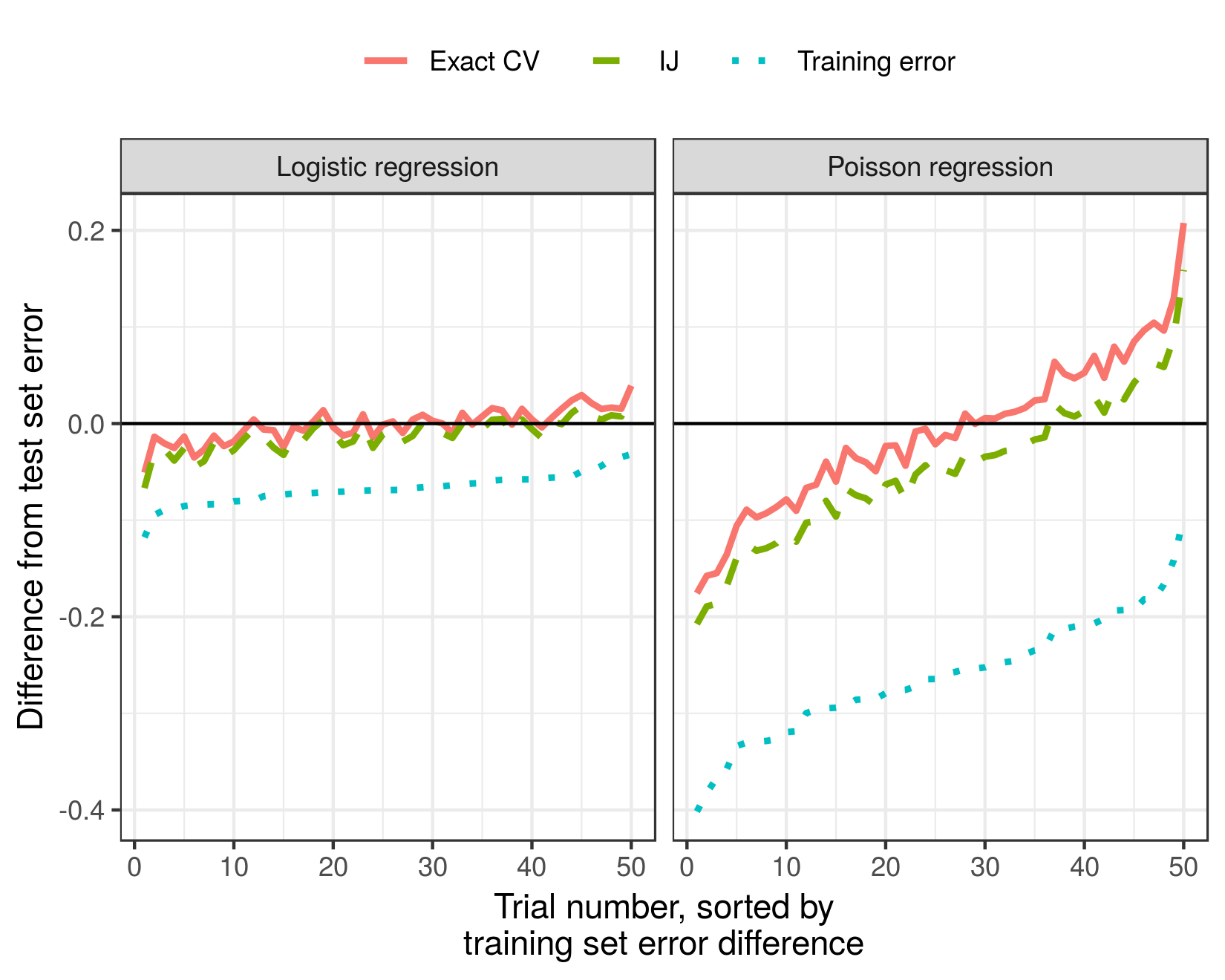
Figure 1: Simulated data: accuracy results.

For a ground truth, we generate a large test set with $N=100{,}000$ datapoints to measure the true generalization error. We show in Fig. 1 that, over 50 randomly generated datasets, our approximation consistently underestimates the actual error predicted by exact leave-one-out CV; however, the difference is small relative to the improvements they both make over the error evaluated on the training set.

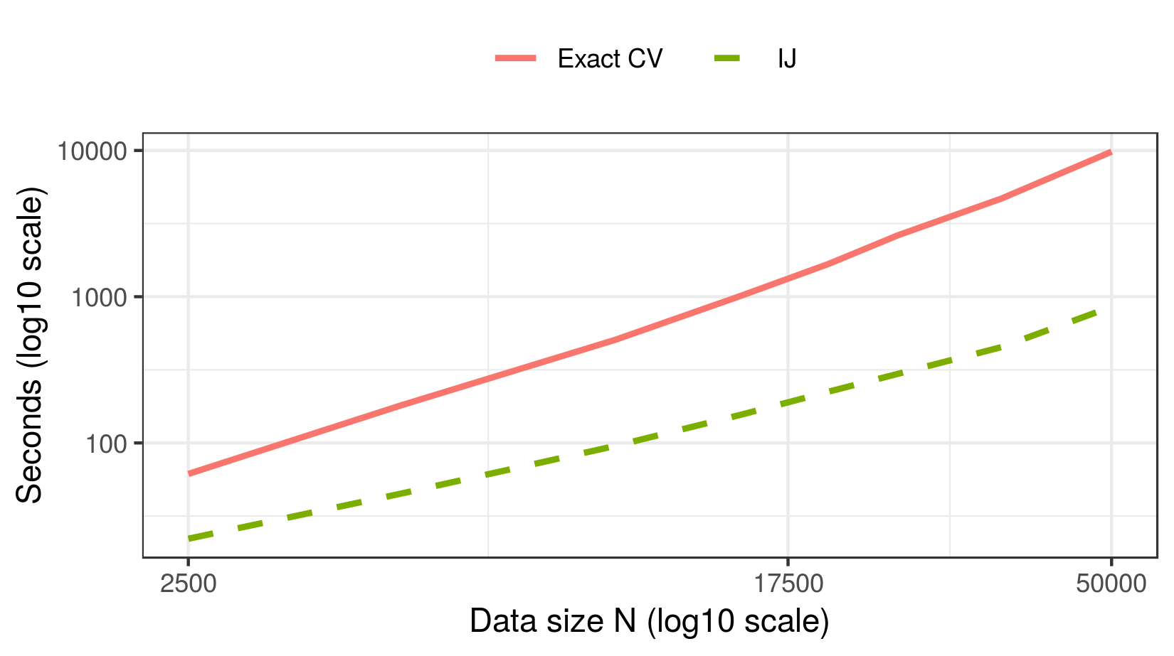
Figure 2: Simulated data: timing results.

Fig. 2 shows the relative timings of our approximation and exact leave-one-out CV on logistic regression with datasets of increasing size. The time to run our approximation is roughly an order of magnitude smaller.

6 Genomics Experiments

We now consider a genomics application in which we use CV to choose the degree of a spline smoother when clustering time series of gene expression data. Code and instructions to reproduce our results can be found in the git repository rgiordan/AISTATS2019SwissArmyIJ. The application is also described in detail in Appendix B.

We use a publicly available data set of mice gene expression (Shoemaker et al., 2015) in which mice were infected with influenza virus, and gene expression was assessed several times after infection. The observed data consists of expression levels $y_{gt}$ for genes $g=1,\ldots,n_{g}$ and time points $t=1,\ldots,n_{t}$. In our case $n_{g}=1000$ and $n_{t}=14$. Many genes behave the same way; thus, clustering the genes by the pattern of their behavior over time allows dimensionality reduction that can facilitate interpretation. Consequently, we wish to first fit a smoothed regression line to each gene and then cluster the results. Following Luan and Li (2003), we model the time series as a gene-specific constant additive offset plus a B-spline basis of degree $3$, and the task is to choose the B-spline basis degrees of freedom using cross-validation on the time points.

Our analysis runs in two stages—first, we regress the genes on the spline basis, and then we cluster a transformed version of the regression fits. By modeling in two stages, we both speed up the clustering and allow for the use of flexible transforms of the fits. We are interested in choosing the smoothing parameter using CV on the time points. Both the time points and the smoothing parameter enter the regression objective directly, but they affect the clustering objective only through the optimal regression parameters. Because the optimization proceeds in two stages, the fit is not the optimum of any single objective function. However, it can still be represented as an M-estimator (see Appendix B).

We implemented the model in scipy (Jones et al., 2001) and computed all derivatives with autograd (Maclaurin et al., 2015). We note that the match between “exact” cross-validation (removing time points and re-optimizing) and the IJ was considerably improved by using a high-quality second-order optimization method. In particular, for these experiments, we employed the Newton conjugate-gradient trust region method (Wright and Nocedal, 1999, Chapter 7.1) as implemented by the method trust-ncg in scipy.optimize, preconditioned by the Cholesky decomposition of an inverse Hessian calculated at an initial approximate optimum. The Hessian used for the preconditioner was with respect to the clustering parameters only and so could be calculated quickly, in contrast to the $H_{1}$ matrix used for the IJ, which includes the regression parameters as well. We found that first-order or quasi-Newton methods (such as BFGS) often got stuck or terminated at points with fairly large gradients. At such points our method does not apply in theory nor, we found, very well in practice.

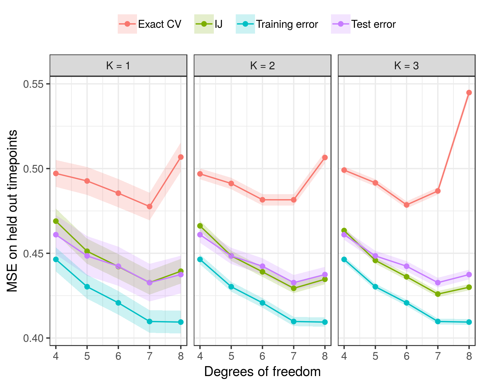
Figure 3: Genomics data: accuracy results.

Fig. 3 shows that the IJ is a reasonably good approximation to the test set error. In particular, both the IJ and exact CV capture the increase in test error for $df=8$, which is not present in the training error. Thus we see that, like exact CV, the IJ is able to prevent overfitting. Though the IJ underestimates exact CV, we note that it differs from exact CV by no more than exact CV itself differs from the true quantity of iterest, the test error.

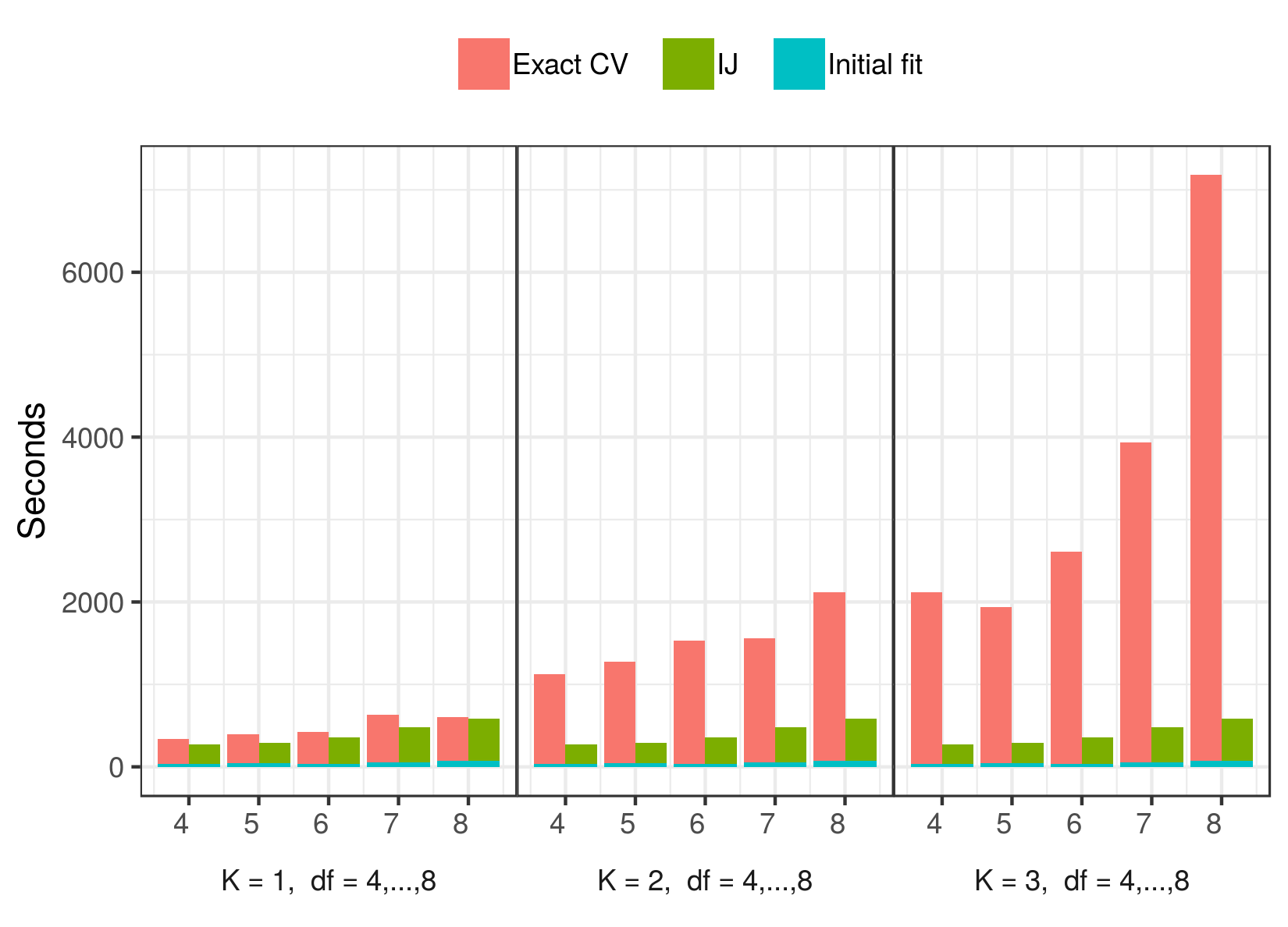
Figure 4: Genomics data: timing results.

The timing results for the genomics experiment are shown in Fig. 4. For this particular problem with approximately $39,000$ parameters (the precise number depends on the degrees of freedom), finding the initial optimum takes about $42$ seconds. The cost of finding the initial optimum is shared by exact CV and the IJ, and, as shown in Fig. 4, is a small proportion of both.

The principle time cost of the IJ is the computation of $H_{1}$. Computing and inverting a dense matrix of size $39,000$ would be computationally prohibitive. But, for the regression objective, $H_{1}$ is extremely sparse and block diagonal, so computing $H_{1}$ in this case took only around $360$ seconds. Inverting $H_{1}$ took negligible time. Once we have $H_{1}^{-1}$, obtaining the subsequent IJ approximations is nearly instantaneous.

The cost of refitting the model for exact CV varies by degrees of freedom (increasing degrees of freedom increases the number of parameters) and the number of left-out points (an increasing number of left-out datapoints increases the number of refits). As can be seen in Fig. 4, for low degrees of freedom and few left-out points, the cost of re-optimizing is approximately the same as the cost of computing $H_{1}$. However, as the degrees of freedom and number of left-out points grow, the cost of exact CV increases to as much as an order of magnitude more than that of the IJ.

7 Conclusion

We recommend consideration of the Swiss Army infinitesimal jackknife for modern machine learning problems. The large size of modern data both increases the need for fast approximations and renders such approximations more accurate. Furthermore, modern automatic differentiation renders many past practical difficulties obsolete. By stepping back from the strict requirements of classical statistical theory, we can see that the value of the infinitesimal jackknife extends beyond its traditional application areas, while retaining desirable generality in other respects.

Acknowledgements.

We thank anonymous reviewers for their helpful comments and suggestions. We are grateful to Nelle Varoquaux for her help with the genomics experiments and to Pang Wei Koh for pointing out and helping to correct an error in an earlier version of our proofs. This research was supported in part by DARPA (FA8650-18-2-7832), an ARO YIP award, an NSF CAREER award, and the CSAIL-MSR Trustworthy AI Initiative. Ryan Giordano was supported by the Gordon and Betty Moore Foundation through Grant GBMF3834 and by the Alfred P. Sloan Foundation through Grant 2013-10-27 to the University of California, Berkeley. Runjing Liu was supported by the NSF Graduate Research Fellowship.

Appendix A Detailed assumptions, lemmas, and proofs

A.1 Tools

We begin by stating two general propositions that will be useful. First, we show that a version of Cauchy-Schwartz can be applied to weighted sums of tensors.

Proposition 1.

Tensor array version of Hölder’s inequality. Let $w$ be an array of scalars and let $a=\left(a_{1},...,a_{N}\right)$ be an array of tensors, were each $a_{n}$ is indexed by $i=1,\ldots,D_{A}$ ($i$ may be a multi-index—e.g., if $A$ is a $D\times D$ matrix, then $i=\left(j,k\right)$, for $j,k\in\left[D\right]$ and $D_{A}=D^{2}$). Let $p,q\in\left[1,\infty\right]$ be two numbers such that $p^{-1}+q^{-1}=1$. Then

$$\left\|\frac{1}{N}\sum_{n=1}^{N}w_{n}a_{n}\right\|_{1} \leq\frac{D_{A}^{\frac{1}{p}}}{N}\left\|w\right\|_{p}\left\|a\right\|_{q}.$$

In particular, with $p=q=2$,

$$\left\|\frac{1}{N}\sum_{n=1}^{N}w_{n}a_{n}\right\|_{1} \leq\sqrt{D_{A}}\frac{\left\|w\right\|_{2}}{\sqrt{N}}\frac{\left\|a\right\|_{2}}{\sqrt{N}}.$$

Proof.

The conclusion follows from the ordinary Hölder’s inequality applied term-wise to $n$ and Jensen’s inequality applied to the indices $i$.

$$\left\|\frac{1}{N}\sum_{n=1}^{N}w_{n}a_{n}\right\|_{1} =\sum_{i=1}^{D_{A}}\left|\frac{1}{N}\sum_{n=1}^{N}w_{n}\left(a_{n}\right)_{i}\right|$$

$$\leq\frac{1}{N}\sum_{i=1}^{D_{A}}\left|\left(\sum_{n=1}^{N}\left|w_{n}\right|^{p}\right)^{\frac{1}{p}}\left(\sum_{n=1}^{N}\left|\left(a_{n}\right)_{i}\right|^{q}\right)^{\frac{1}{q}}\right|\text{(H{\"{o}}lder)}$$

$$=\frac{1}{N}\left\|w\right\|_{p}\frac{D_{A}}{D_{A}}\sum_{i=1}^{D_{A}}\left(\sum_{n=1}^{N}\left|\left(a_{n}\right)_{i}\right|^{q}\right)^{\frac{1}{q}}$$

$$\leq\frac{1}{N}\left\|w\right\|_{p}D_{A}\left(\frac{1}{D_{A}}\sum_{i=1}^{D_{A}}\sum_{n=1}^{N}\left|\left(a_{n}\right)_{i}\right|^{q}\right)^{\frac{1}{q}}\textrm{ (Jensen applied to }i\textrm{)}$$

$$=\frac{1}{N}\left\|w\right\|_{p}D_{A}\left(\frac{1}{D_{A}}\sum_{n=1}^{N}\left\|a_{n}\right\|_{q}^{q}\right)^{\frac{1}{q}}$$

$$=\frac{1}{N}\left\|w\right\|_{p}D_{A}^{1-\frac{1}{q}}\left\|a\right\|_{q}$$

$$=\frac{D_{A}^{\frac{1}{p}}}{N}\left\|w\right\|_{p}\left\|a\right\|_{q}.$$

∎

Next, we prove a relationship between the term-wise difference between matrices and the difference between their operator norms. It is well-known that the minimum eigenvalue of a non-singular matrix is continuous in the entries of the matrix. In the next proposition, we quantify this continuity for the $L_{1}$ norm.

Proposition 2.

Let $A$ and $B$ be two square matrices of the same size. Let $\left\|A^{-1}\right\|_{op}\leq C_{op}^{\text{\,}}$ for some finite $C_{op}^{\text{\,}}$, and Then

$$\left\|A-B\right\|_{1}\leq\frac{1}{2}(C_{op}^{\text{\,}})^{-1} \quad\Rightarrow\quad\left\|B^{-1}\right\|_{op}\leq 2C_{op}^{\text{\,}}.$$

Proof.

We will use the results stated in Theorem 4.29 of Schott [2016] and the associated discussion in Example 4.14, which establish the following result. Let $A$ be a square, nonsigular matrix, and let $I$ be the identity matrix of the same size. Let $\left\|\cdot\right\|$ denote any matrix norm satisfying $\left\|I\right\|=1$. Let $D$ be a matrix of the same size as $A$ satisfying

$$\eqlabel{ab_{m}atrix_{c}ondition}\left\|A^{-1}\right\|\left\|D\right\|\leq 1.$$ (2)

Then

$$\left\|A^{-1}-(A+D)^{-1}\right\|\leq\frac{\left\|A^{-1}\right\|\left\|D\right\|}{1-\left\|A^{-1}\left\|D\right\|\right\|}\left\|A^{-1}\right\|.$$ (3)

We will apply (LABEL:matrix_norm_continuity) using the operator norm $\left\|\cdot\right\|_{op}$, for which $\left\|I\right\|_{op}=1$ and with $D:=B-A$. Because $\left\|A^{-1}\right\|_{op}\leq C_{op}^{\text{\,}}$, $A$ is invertible.

Assume that $\left\|A-B\right\|_{1}\leq\frac{1}{2}(C_{op}^{\text{\,}})^{-1}$. First, note that

$$\left\|A^{-1}\right\|_{op}\left\|D\right\|_{op} =\left\|A^{-1}\right\|_{op}\left\|B-A\right\|_{op}$$

$$\leq\left\|A^{-1}\right\|_{op}\left\|B-A\right\|_{1}$$ (ordering of matrix norms)

$$\leq C_{op}^{\text{\,}}\frac{1}{2}(C_{op}^{\text{\,}})^{-1}$$ (by assumption)

$$=\frac{1}{2}<1,$$ (4)

so (LABEL:ab_matrix_condition) is satisfied and we can apply (LABEL:matrix_norm_continuity). Then

$$\left\|B^{-1}\right\|_{op} \leq\left\|B^{-1}-A^{-1}\right\|_{op}+\left\|A^{-1}\right\|_{op}$$ (triangle inequality)

$$\leq\frac{\left\|A^{-1}\right\|_{op}\left\|B-A\right\|_{op}}{1-\left\|A^{-1}\right\|_{op}\left\|B-A\right\|_{op}}\left\|A^{-1}\right\|_{op}+\left\|A^{-1}\right\|_{op}$$ ((LABEL:matrix_norm_continuity))

$$\leq\frac{\frac{1}{2}}{1-\frac{1}{2}}\left\|A^{-1}\right\|_{op}+\left\|A^{-1}\right\|_{op}$$ ((LABEL:ab_matrix_condition_fulfilled))

$$\leq 2C_{op}^{\text{\,}}.$$ (by assumption)

∎

Next, we define the quantities needed to make use of the integral form of the Taylor series remainder.

Proposition 3.

For any $\theta\in\Omega_{\theta}$ and any $\tilde{w}\in W$,

$$G(\theta,\tilde{w})-G(\hat{\theta}_{1},\tilde{w})= \left(\int_{0}^{1}H(\hat{\theta}_{1}+t(\theta-\hat{\theta}_{1}),w)dt\right)\left(\theta-\hat{\theta}_{1}\right)$$

Proof.

Let $G_{d}(\theta,\tilde{w})$ denote the $d$-th component of the vector $G(\theta,\tilde{w})$, and define the function $f_{d}(t):=G_{d}(\hat{\theta}_{1}+t(\hat{\theta}_{1}-\theta),\tilde{w})$. The proposition follows by taking the integral remainder form of the zero-th order Taylor series expansion of $f_{d}(t)$ around $t=0$ [Dudley, 2018, Appendix B.2], and stacking the result into a vector. ∎

The Taylor series residual of 3 will show up repeatedly, so we will give it a concise name in the following definition.

Definition 4.

For a fixed weight $w$ and a fixed parameter $\theta$, define the Hessian integral

$$\tilde{H}(\theta,w):= \int_{0}^{1}H(\hat{\theta}_{1}+t(\theta-\hat{\theta}_{1}),w)dt.$$

A.2 Lemmas

We now prove some useful consequences of our assumptions. The proof roughly proceeds for all $w\in W_{\delta}$ by the following steps:

1. When $\delta$ is small we can make $\left\|{{\hat{\theta}\left(w\right)}}-\hat{\theta}_{1}\right\|_{2}$ small. (3 below.)

2. When $\left\|\theta-\hat{\theta}_{1}\right\|_{2}$ is small, then the derivatives $H\left(\theta,w\right)$ are close to their optimal value, $H\left(\hat{\theta}_{1},1_{w}\right)$. (4 and 5 below.)

3. When the derivatives are close to their optimal values, then $H\left(\theta,w\right)$ is uniformly non-singular. (6 below.)

4. When the derivatives are close to their optimal values and $H\left(\theta,w\right)$ is uniformly non-singular we can control the error in $\hat{\theta}_{\textrm{IJ}}-\hat{\theta}\left(w\right)$ in terms of $\delta$. (2 below.)

We begin by showing that the difference between $\hat{\theta}\left(w\right)$ and $\hat{\theta}_{1}$ for $w\in W_{\delta}$ can be made small by making $\delta$ from 1 small. First, however, we need to prove that operator norm bounds on $H(\theta,w)$ also apply to the integrated Hessian $\tilde{H}(\theta,w)$.

Lemma 2.

Invertibility of the integrated Hessian. If, for some domain $\Omega$ and some constant $C$, $\sup_{\theta\in\Omega}\left\|H(\theta,w)^{-1}\right\|_{op}\leq C$, then $\sup_{\theta\in\Omega}\left\|\tilde{H}(\theta,w)^{-1}\right\|_{op}\leq C$.

Proof.

By definition of the operator norm,

$$\left\|\tilde{H}(\theta,w)^{-1}\right\|_{op}^{-1}= \min_{v\in\mathbb{R}^{D}:\left\|v\right\|_{2}=1}v^{T}\tilde{H}(\theta,w)v$$

$$= \min_{v\in\mathbb{R}^{D}:\left\|v\right\|_{2}=1}\int_{0}^{1}v^{T}H(\hat{\theta}_{1}+t(\theta-\hat{\theta}_{1}),w)vdt$$

$$\geq \int_{0}^{1}\min_{v\in\mathbb{R}^{D}:\left\|v\right\|_{2}=1}v^{T}H(\hat{\theta}_{1}+t(\theta-\hat{\theta}_{1}),w)vdt$$

$$\geq \inf_{\theta\in\Omega}\min_{v\in\mathbb{R}^{D}:\left\|v\right\|_{2}=1}v^{T}H(\theta,w)v$$

$$\geq C^{-1}.$$

The result follows by inverting both sides of the inequality. ∎

Lemma 3.

Small parameter changes. Under Assumptions 1—3 and 1,

$$\textrm{for all }w\in W_{\delta},\quad\left\|{{\hat{\theta}\left(w\right)}}-\hat{\theta}_{1}\right\|_{2} \leq C_{op}^{\text{\,}}\delta.$$

Proof.

Applying 3 with $\theta=\hat{\theta}\left(w\right)$ and $\tilde{w}=1_{w}$ gives

$$G\left(\hat{\theta}\left(w\right),1_{w}\right) =G\left(\hat{\theta}_{1},1_{w}\right)+\tilde{H}\left(\hat{\theta}\left(w\right),1_{w}\right)\left(\hat{\theta}\left(w\right)-\hat{\theta}_{1}\right).$$

By 2 and 2, $\sup_{\theta\in\Omega_{\theta}}\left\|\tilde{H}(\theta,1_{w})^{-1}\right\|\leq C_{op}^{\text{\,}}$. In particular, $\tilde{H}(\theta,1_{w})$ is non-singular. A little manipulation, together with the fact that $G\left(\hat{\theta}\left(w\right),w\right)=G\left(\hat{\theta}_{1},1_{w}\right)=0$ gives

$$\hat{\theta}\left(w\right)-\hat{\theta}_{1} =\tilde{H}\left(\hat{\theta}\left(w\right),1_{w}\right)^{-1}\left(G\left(\hat{\theta}\left(w\right),1_{w}\right)-G\left(\hat{\theta}\left(w\right),w\right)\right).$$

Taking the norm of both sides gives

$$\left\|{{\hat{\theta}\left(w\right)}}-\hat{\theta}_{1}\right\|_{2} =\left\|\tilde{H}\left(\hat{\theta}\left(w\right),1_{w}\right)^{-1}\left(G\left({{\hat{\theta}\left(w\right)}},1_{w}\right)-G\left({{\hat{\theta}\left(w\right)}},w\right)\right)\right\|_{2}$$

$$\leq\left\|\tilde{H}\left(\hat{\theta}\left(w\right),1_{w}\right)^{-1}\right\|_{op}\left\|\left(G\left({{\hat{\theta}\left(w\right)}},1_{w}\right)-G\left({{\hat{\theta}\left(w\right)}},w\right)\right)\right\|_{2}$$

$$\leq C_{op}^{\text{\,}}\left\|G\left({{\hat{\theta}\left(w\right)}},1_{w}\right)-G\left({{\hat{\theta}\left(w\right)}},w\right)\right\|_{2}\textrm{ (Lemma \ref{lem:hess_integral_invertible})}$$

$$\leq C_{op}^{\text{\,}}\left\|G\left({{\hat{\theta}\left(w\right)}},1_{w}\right)-G\left({{\hat{\theta}\left(w\right)}},w\right)\right\|_{1}\textrm{ (relation between norms)}$$

$$\leq C_{op}^{\text{\,}}\sup_{\theta\in\Omega_{\theta}}\left\|G\left(\theta,1_{w}\right)-G\left(\theta,w\right)\right\|_{1}$$

$$\leq C_{op}^{\text{\,}}\delta.\textrm{ (Condition \ref{cond:paper_uniform_bound}).}$$

∎

Because we will refer to it repeatedly, we give the set of $\theta$ defined in 3 a name.

Definition 5.

For a given $\delta$, define the region around $\hat{\theta}_{1}$ given by 3 as

$$B_{C_{op}\delta} :=\left\{\theta:\left\|\theta-\hat{\theta}_{1}\right\|_{2}\leq C_{op}^{\text{\,}}\delta\right\}\bigcap\Omega_{\theta}.$$

In other words, 3 states that 1 implies $\hat{\theta}\left(w\right)\in B_{C_{op}\delta}$ when $w\in W_{\delta}$.

Next, we show that closeness in $\theta$ will mean closeness in $H\left(\theta,w\right)$.

Lemma 4.

Boundedness and continuity. Under Assumptions 1–5 and 1,

$$\textrm{for all }\theta\in B_{\Delta_{\theta}},\quad\sup_{w\in W}\left\|H\left(\theta,w\right)-H\left(\hat{\theta}_{1},w\right)\right\|_{1} \leq DC_{w}L_{h}\left\|\theta-\hat{\theta}_{1}\right\|_{2}.$$

Proof.

For $\theta\in B_{\Delta_{\theta}}$,

$$\sup_{w\in W}\left\|H\left(\theta,w\right)-H\left(\hat{\theta}_{1},w\right)\right\|_{1} =\sup_{w\in W}\left\|\frac{1}{N}\sum_{n=1}^{N}w_{n}\left(h_{n}\left(\theta\right)-h_{n}\left(\hat{\theta}_{1}\right)\right)\right\|_{1}\textrm{ (by definition)}$$

$$\leq D\sup_{w\in W}\frac{\left\|w\right\|_{2}}{\sqrt{N}}\frac{\left\|h\left(\theta\right)-h\left(\hat{\theta}_{1}\right)\right\|_{2}}{\sqrt{N}}\textrm{ (Proposition \ref{propref:tensor_cauchy_schwartz})}$$

$$\leq DC_{w}\frac{\left\|h\left(\theta\right)-h\left(\hat{\theta}_{1}\right)\right\|_{2}}{\sqrt{N}}\textrm{ (Assumption \ref{assu:paper_weight_bounded})}$$

$$\leq DC_{w}L_{h}\left\|\theta-\hat{\theta}_{1}\right\|_{2}\textrm{ (Assumption \ref{assu:paper_lipschitz} and }\theta\in B_{\Delta_{\theta}}\textrm{)}.$$

∎

We now combine 3 and 4 to show that $H\left(\theta,w\right)$ is close to its value at the solution $H\left(\hat{\theta}_{1},1_{w}\right)$ for sufficiently small $\delta$ and for all $\theta\in B_{C_{op}\delta}$.

Lemma 5.

Bounds for difference in parameters. Under Assumptions 1–5 and 1, if $\delta\leq\Delta_{\theta}C_{op}^{-1}$, then

$$\sup_{\theta\in B_{C_{op}\delta}}\sup_{w\in W_{\delta}} \left\|H\left(\theta,w\right)-H\left(\hat{\theta}_{1},1_{w}\right)\right\|_{1}\leq\left(1+DC_{w}L_{h}C_{op}^{\text{\,}}\right)\delta.$$

Proof.

By 3, $\delta\leq\Delta_{\theta}C_{op}^{-1}$ implies that $C_{op}^{\text{\,}}\delta\leq\Delta_{\theta}$ and so $B_{C_{op}\delta}\subseteq B_{\Delta_{\theta}}$. Consequently, we can apply 4:

$$\sup_{\theta\in B_{C_{op}\delta}}\sup_{w\in W_{\delta}}\left\|H\left(\theta,w\right)-H\left(\hat{\theta}_{1},w\right)\right\|_{1} \leq\sup_{\theta\in B_{\Delta_{\theta}}}\sup_{w\in W_{\delta}}\left\|H\left(\theta,w\right)-H\left(\hat{\theta}_{1},w\right)\right\|_{1}$$

$$\leq DC_{w}L_{h}\left\|\theta-\hat{\theta}_{1}\right\|_{2}\textrm{ (Lemma \ref{lem:bounded_continuous})}$$

$$\leq DC_{w}L_{h}C_{op}^{\text{\,}}\delta\quad\textrm{ (because }\theta\in B_{C_{op}\delta}\textrm{)}.$$

Next, we can use this to write

$$\sup_{\theta\in B_{C_{op}\delta}}\sup_{w\in W_{\delta}} \left\|H\left(\theta,w\right)-H\left(\hat{\theta}_{1},1_{w}\right)\right\|_{1}$$

$$=\sup_{\theta\in B_{C_{op}\delta}}\sup_{w\in W_{\delta}}\left\|H\left(\theta,w\right)-H\left(\theta,1_{w}\right)+H\left(\theta,1_{w}\right)-H\left(\hat{\theta}_{1},1_{w}\right)\right\|_{1}$$

$$\leq\sup_{\theta\in B_{C_{op}\delta}}\sup_{w\in W_{\delta}}\left\|H\left(\theta,w\right)-H\left(\theta,1_{w}\right)\right\|_{1}+\sup_{\theta\in B_{C_{op}\delta}}\sup_{w\in W_{\delta}}\left\|H\left(\theta,1_{w}\right)-H\left(\hat{\theta}_{1},1_{w}\right)\right\|_{1}$$

$$\leq\sup_{\theta\in\Omega_{\theta}}\sup_{w\in W_{\delta}}\left\|H\left(\theta,w\right)-H\left(\theta,1_{w}\right)\right\|_{1}+\sup_{\theta\in B_{C_{op}\delta}}\sup_{w\in W_{\delta}}\left\|H\left(\theta,1_{w}\right)-H\left(\hat{\theta}_{1},1_{w}\right)\right\|_{1}$$

$$\leq\delta+\sup_{\theta\in B_{C_{op}\delta}}\sup_{w\in W_{\delta}}\left\|H\left(\theta,1_{w}\right)-H\left(\hat{\theta}_{1},1_{w}\right)\right\|_{1}\textrm{ (Condition \ref{cond:paper_uniform_bound})}$$

$$\leq\delta+DC_{w}L_{h}C_{op}^{\text{\,}}\delta.$$

∎

The constant that appears multiplying $\delta$ at the end of the proof of 5 will appear often in what follows, so we give it the special name $C_{\textrm{IJ}}$ in 3.

Note that 5 places a condition on how small $\delta$ must be in order for our regularity conditions to apply. 3 will guarantee that $\hat{\theta}\left(w\right)\in B_{C_{op}\delta}$, but if we are not able to make $\delta$ arbitrarily small in 1, then we are not guaranteed to ensure that $B_{C_{op}\delta}\subseteq B_{\Delta_{\theta}}$, will not be able to assume Lipschitz continuity, and none of our results will apply.

Next, using 5, we can extend the operator bound on $H_{1}^{-1}$ from 2 to $H\left(\theta,w\right)^{-1}$ for all $w\in W_{\delta}$.

Lemma 6.

Uniform invertibility of the Hessian. Under Assumptions 1–5 and 1, if $\delta\leq\min\left\{\Delta_{\theta}C_{op}^{-1},\frac{1}{2}C_{\textrm{IJ}}^{-1}C_{op}^{-1}\right\}$, then

$$\sup_{\theta\in B_{C_{op}\delta}}\sup_{w\in W_{\delta}}\left\|H\left(\theta,w\right)^{-1}\right\|_{op} \leq 2C_{op}^{\text{\,}}.$$

Proof.

By 2, $\left\|H\left(\hat{\theta}_{1},1_{w}\right)^{-1}\right\|_{op}\leq C_{op}^{\text{\,}}$. So by 2, it will suffice to select $\delta$ so that

$$\sup_{\theta\in B_{C_{op}\delta}}\sup_{w\in W_{\delta}}\left\|H\left(\theta,w\right)-H\left(\hat{\theta}_{1},1_{w}\right)\right\|_{1} \leq\frac{1}{2}C_{op}^{-1}.$$ (5)

When we can apply 5, we have

$$\sup_{\theta\in B_{C_{op}\delta}}\sup_{w\in W_{\delta}}\left\|H\left(\theta,w\right)-H\left(\hat{\theta}_{1},1_{w}\right)\right\|_{1} \leq C_{\textrm{IJ}}\delta.$$

So $H\left(\theta,w\right)$ will satisfy (LABEL:h_bound) if we can apply 5 and if

$$\delta\leq \frac{1}{2}C_{op}^{-1}C_{\textrm{IJ}}^{-1}.$$

To apply 5 we additionally require that $\delta\leq\Delta_{\theta}C_{op}^{-1}$. By taking $\delta\leq\min\left\{\Delta_{\theta}C_{op}^{-1},\frac{1}{2}C_{op}^{-1}C_{\textrm{IJ}}^{-1}\right\}$, we satisfy (LABEL:h_bound) and the result follows. ∎

Next, we show that a version of 5 also applies to the integrated Hessian $\tilde{H}(\theta,w)$ when $\theta\in B_{C_{op}\delta}$.

Lemma 7.

Bounds for difference of the integrated Hessian. Under Assumptions 1–5 and 1, if $\delta\leq\Delta_{\theta}C_{op}^{-1}$ and $\theta\in B_{C_{op}\delta}$,

$$\sup_{w\in W_{\delta}}\left\|\tilde{H}\left(\theta,w\right)-H(\hat{\theta}_{1},1_{w})\right\|_{1}\leq \left(1+DC_{w}L_{h}C_{op}^{\text{\,}}\right)\delta.$$

Proof.

$$\sup_{w\in W_{\delta}}\left\|\tilde{H}\left(\theta,w\right)-H(\hat{\theta}_{1},1_{w})\right\|_{1}$$

$$= \sup_{w\in W_{\delta}}\left\|\int_{0}^{1}\left(H(\hat{\theta}_{1}+t(\theta-\hat{\theta}_{1}),w)dt-H(\hat{\theta}_{1},1_{w})\right)\right\|_{1}$$ (Definition 4)

$$\leq \sup_{w\in W_{\delta}}\int_{0}^{1}\left\|H(\hat{\theta}_{1}+t(\theta-\hat{\theta}_{1}),w)-H(\hat{\theta}_{1},1_{w})\right\|_{1}dt$$ (Jensen’s inequality)

$$\leq \sup_{\theta\in B_{C_{op}\delta}}\sup_{w\in W_{\delta}}\left\|H(\theta),w)-H(\hat{\theta}_{1},1_{w})\right\|_{1}$$

$$\leq \left(1+DC_{w}L_{h}C_{op}^{\text{\,}}\right)\delta$$ (Lemma 5)

∎

With these results in hand, the upper bound on $\delta$ will at last be sufficient to control the error terms in our approximation. For compactness, we give it the upper bound on $\delta$ the name $\Delta_{\delta}$ in 3.

Finally, we state a result that will allow us to define derivatives of $\hat{\theta}\left(w\right)$ with respect to $w$.

Lemma 8.

Inverse function theorem. Under Assumptions 1–5 and 1, and for $\delta\leq\Delta_{\delta}$, there exists a continuous, differentiable function of $w$, $\hat{\theta}\left(w\right)$, such that, for all $w\in W$, G$\left(\hat{\theta}\left(w\right),w\right)=0$.

Proof.

This follows from 6 and the implicit function theorem. ∎

By definition, $\hat{\theta}\left(1_{w}\right)=\hat{\theta}_{1}$.

A.3 Bounding the errors in a Taylor expansion

We are now in a position to use Assumptions 1–5 and 1 to bound the error terms in a first-order Taylor expansion of $\hat{\theta}\left(w\right)$. We begin by simply calculating the derivative $d\hat{\theta}\left(w\right)/dw$.

Proposition 4.

For any $w\in W$ for which $H\left(\hat{\theta}\left(w\right),w\right)$ is invertible, and for any vector $a\in\mathbb{R}^{N}$,

$$\frac{d\hat{\theta}\left(w\right)}{dw^{T}}\rvert_{w}a =-H\left(\hat{\theta}\left(w\right),w\right)^{-1}G\left(\hat{\theta}\left(w\right),a\right).$$

Proof.

Because $G\left(\hat{\theta}\left(w\right),w\right)=0$ for all $w\in W$, by direct calculation,

$$0 =\frac{d}{dw^{T}}G\left(\hat{\theta}\left(w\right),w\right)\rvert_{w}a$$

$$=\left(\frac{\partial G}{\partial\theta^{T}}\frac{d\hat{\theta}}{dw^{T}}+\frac{\partial G}{\partial w^{T}}\right)\rvert_{{}_{w}}a$$

$$=H\left(\hat{\theta}\left(w\right),w\right)\frac{d\hat{\theta}}{dw^{T}}\rvert_{{}_{w}}a+\left(\frac{\partial}{\partial w^{T}}\frac{1}{N}\sum_{n=1}^{N}w_{n}g_{n}\left(\theta\right)\right)\rvert_{{}_{w}}a$$

$$=H\left(\hat{\theta}\left(w\right),w\right)\frac{d\hat{\theta}}{dw^{T}}\rvert_{{}_{w}}a+\frac{1}{N}\sum_{n=1}^{N}g_{n}\left(\hat{\theta}\left(w\right)\right)a$$

$$=H\left(\hat{\theta}\left(w\right),w\right)\frac{d\hat{\theta}}{dw^{T}}\rvert_{{}_{w}}a+G\left(\hat{\theta}\left(w\right),a\right).$$

Because $H\left(\hat{\theta}\left(w\right),w\right)$ is invertible by assumption, the result follows. ∎

Definition 6.

Define

$$\hat{\theta}_{\textrm{IJ}}\left(w\right) :=\hat{\theta}_{1}+\frac{d\hat{\theta}\left(w\right)}{dw^{T}}\rvert_{1_{w}}\left(w-1_{w}\right)$$

$$=\hat{\theta}_{1}-H_{1}^{-1}G\left(\hat{\theta}_{1},w\right).\textrm{ (because }G\left(\hat{\theta}_{1},1_{w}\right)=0\textrm{)}$$

$\hat{\theta}_{\textrm{IJ}}\left(w\right)$ in 6 is the first term in a Taylor series expansion of $\hat{\theta}\left(w\right)$ as a function of $w$. We want to bound the error, $\hat{\theta}_{\textrm{IJ}}\left(w\right)-\hat{\theta}\left(w\right)$.

Theorem 2.

Under Assumptions 1–5 and 1, when $\delta\leq\Delta_{\delta}$,

$$\sup_{w\in W_{\delta}}\left\|\hat{\theta}_{\textrm{IJ}}\left(w\right)-\hat{\theta}\left(w\right)\right\|_{2} \leq 2C_{op}^{2}C_{\textrm{IJ}}\delta^{2}.$$

Proof.

Applying 3 with $\theta=\hat{\theta}\left(w\right)$ and $\tilde{w}=w$, we have

$$0=G\left(\hat{\theta}\left(w\right),w\right) =G\left(\hat{\theta}_{1},w\right)+\tilde{H}\left(\hat{\theta}\left(w\right),w\right)\left(\hat{\theta}\left(w\right)-\hat{\theta}_{1}\right).$$

Because $\delta\in W_{\delta}$, 3 implies that $\hat{\theta}\left(w\right)\in B_{C_{op}\delta}$ so, 6 and 2 imply that $\tilde{H}\left(\hat{\theta}\left(w\right),w\right)$ is invertible and we can solve for $\hat{\theta}\left(w\right)-\hat{\theta}_{1}$.

$$\hat{\theta}\left(w\right)-\hat{\theta}_{1} =-\tilde{H}\left(\hat{\theta}\left(w\right),w\right)^{-1}G\left(\hat{\theta}_{1},w\right)$$

$$=\left(-\tilde{H}\left(\tilde{\theta},w\right)^{-1}+H\left(\hat{\theta}_{1},1_{w}\right)^{-1}-H\left(\hat{\theta}_{1},1_{w}\right)^{-1}\right)G\left(\hat{\theta}_{1},w\right)$$

$$=\left(H\left(\hat{\theta}_{1},1_{w}\right)^{-1}-\tilde{H}\left(\hat{\theta}\left(w\right),w\right)^{-1}\right)G\left(\hat{\theta}_{1},w\right)+\hat{\theta}_{\textrm{IJ}}\left(w\right)-\hat{\theta}_{1}.$$

Eliminating $\hat{\theta}_{1}$ and taking the supremum of both sides gives

$$\sup_{w\in W_{\delta}} \left\|\hat{\theta}_{\textrm{IJ}}\left(w\right)-{{\hat{\theta}\left(w\right)}}\right\|_{2}$$

$$=\sup_{w\in W_{\delta}}\left\|\left(H\left(\hat{\theta}_{1},1_{w}\right)^{-1}-\tilde{H}\left(\theta,w\right)^{-1}\right)G\left(\hat{\theta}_{1},w\right)\right\|_{2}$$

$$=\sup_{w\in W_{\delta}}\left\|\tilde{H}\left(\hat{\theta}\left(w\right),w\right)^{-1}\left(\tilde{H}\left(\hat{\theta}\left(w\right),w\right)-H\left(\hat{\theta}_{1},1_{w}\right)\right)H\left(\hat{\theta}_{1},1_{w}\right)^{-1}G\left(\hat{\theta}_{1},w\right)\right\|_{2}$$

$$\leq 2C_{op}^{\text{\,}}\sup_{w\in W_{\delta}}\left\|\left(\tilde{H}\left(\hat{\theta}\left(w\right),w\right)-H\left(\hat{\theta}_{1},1_{w}\right)\right)H\left(\hat{\theta}_{1},1_{w}\right)^{-1}G\left(\hat{\theta}_{1},w\right)\right\|_{2}\textrm{ (Lemma \ref{lem:hess_integral_invertible})}$$

$$\leq 2C_{op}^{\text{\,}}\sup_{w\in W_{\delta}}\left\|\tilde{H}\left(\hat{\theta}\left(w\right),w\right)-H\left(\hat{\theta}_{1},1_{w}\right)\right\|_{op}\left\|H\left(\hat{\theta}_{1},1_{w}\right)^{-1}G\left(\hat{\theta}_{1},w\right)\right\|_{2}$$

$$\leq 2C_{op}^{\text{\,}}\sup_{w\in W_{\delta}}\left\|\tilde{H}\left(\hat{\theta}\left(w\right),w\right)-H\left(\hat{\theta}_{1},1_{w}\right)\right\|_{1}\left\|H\left(\hat{\theta}_{1},1_{w}\right)^{-1}G\left(\hat{\theta}_{1},w\right)\right\|_{2}\textrm{ (ordering of matrix norms)}$$

$$\leq 2C_{op}^{\text{\,}}C_{\textrm{IJ}}\delta\sup_{w\in W_{\delta}}\left\|H\left(\hat{\theta}_{1},1_{w}\right)^{-1}G\left(\hat{\theta}_{1},w\right)\right\|_{2}\textrm{ (Lemma \ref{lem:int_h_difference_from_one})}$$

$$\leq 2C_{op}^{2}C_{\textrm{IJ}}\delta\sup_{w\in W_{\delta}}\left\|G\left(\hat{\theta}_{1},w\right)\right\|_{2}\textrm{ (Assumption \ref{assu:paper_hessian})}$$

$$=2C_{op}^{2}C_{\textrm{IJ}}\delta\sup_{w\in W_{\delta}}\left\|G\left(\hat{\theta}_{1},w\right)-G\left(\hat{\theta}_{1},1_{w}\right)\right\|_{2}\textrm{ (because }G\left(\hat{\theta}_{1},1_{w}\right)=0\textrm{)}$$

$$\leq 2C_{op}^{2}C_{\textrm{IJ}}\delta^{2}\textrm{ (Condition \ref{cond:paper_uniform_bound})}.$$

∎

A.4 Use cases

First, let us state a simple condition under which Assumptions 1–4 hold. It will help to have a lemma for the Lipschitz continuity.

Lemma 9.

Derivative Cauchy Schwartz. Let $a\left(\theta\right)=\left(a_{1}\left(\theta\right),...,a_{N}\left(\theta\right)\right)$ be an array of tensors with multi-index $i\in\left[D_{A}\right]$, and let $\frac{\partial a\left(\theta\right)}{\partial\theta}=\left(\frac{\partial}{\partial\theta}a_{1}\left(\theta\right),...,\frac{\partial}{\partial\theta}a_{N}\left(\theta\right)\right)$ be an array of tensors of size $D\times D_{A}$. Then

$$\left\|\frac{\partial}{\partial\theta}\left\|a\left(\theta\right)\right\|_{2}\right\|_{2} \leq D_{A}\left\|\frac{\partial a}{\partial\theta}\right\|_{2}.$$

Proof.

By direct calculation,

$$\left\|\frac{\partial}{\partial\theta}\left\|a\left(\theta\right)\right\|_{2}^{2}\right\|_{2}^{2} =\sum_{r=1}^{D}\left(\frac{\partial}{\partial\theta_{r}}\sum_{n=1}^{N}\sum_{i=1}^{D_{A}}a_{n,i}\left(\theta\right)^{2}\right)^{2}$$

$$=\sum_{r=1}^{D}\left(\sum_{n=1}^{N}\sum_{i=1}^{D_{A}}2a_{n,i}\left(\theta\right)\frac{\partial a_{n,i}\left(\theta\right)}{\partial\theta_{r}}\right)^{2}$$

$$\leq\sum_{r=1}^{D}\left(2\sum_{i=1}^{D_{A}}\left(\sum_{n=1}^{N}a_{n,i}\left(\theta\right)^{2}\right)^{\frac{1}{2}}\left(\sum_{n=1}^{N}\left(\frac{\partial a_{n,i}\left(\theta\right)}{\partial\theta_{r}}\right)^{2}\right)^{\frac{1}{2}}\right)^{2}$$

$$\leq\sum_{r=1}^{D}\left(2D_{A}^{2}\left(\frac{1}{D_{A}}\sum_{i=1}^{D_{A}}\sum_{n=1}^{N}a_{n,i}\left(\theta\right)^{2}\right)^{\frac{1}{2}}\left(\frac{1}{D_{A}}\sum_{n=1}^{N}\left(\frac{\partial a_{n,i}\left(\theta\right)}{\partial\theta_{r}}\right)^{2}\right)^{\frac{1}{2}}\right)^{2}$$

$$=4D_{A}^{2}\left\|a\right\|_{2}^{2}\sum_{r=1}^{D}\left\|\frac{\partial a}{\partial\theta_{r}}\right\|_{2}^{2}$$

$$=4D_{A}^{2}\left\|a\right\|_{2}^{2}\left\|\frac{\partial a}{\partial\theta}\right\|_{2}^{2}.$$

By the chain rule,

$$\left\|\frac{\partial}{\partial\theta}\left\|a\left(\theta\right)\right\|_{2}\right\|_{2}^{2} =\frac{1}{4\left\|a\left(\theta\right)\right\|_{2}^{2}}\left\|\frac{\partial}{\partial\theta}\left\|a\left(\theta\right)\right\|_{2}^{2}\right\|_{2}^{2}\leq D_{A}^{2}\left\|\frac{\partial a}{\partial\theta}\right\|_{2}^{2}.$$

∎

Lemma 10.

Let $a\left(\theta\right)\in\mathbb{R}^{D\times D}$ be a continuously differentiable random matrix with a $D\times D\times D$ derivative tensor. (Note that the function, not $\theta$, is random. For example, $\mathbb{E}\left[a\left(\theta\right)\right]$ is still a function of $\theta$.) Suppose that $\mathbb{E}\left[\left\|a\left(\theta\right)\right\|_{2}\right]$ is finite for all $\theta\in\Omega_{\theta}$. Then, for all $\theta_{1},\theta_{2}\in\Omega_{\theta}$,

$$\left|\mathbb{E}\left[\left\|a\left(\theta_{1}\right)\right\|_{2}\right]-\mathbb{E}\left[\left\|a\left(\theta_{2}\right)\right\|_{2}\right]\right| \leq\sqrt{\mathbb{E}\left[\sup_{\theta\in\Omega_{\theta}}\left\|\frac{\partial a\left(\theta\right)}{\partial\theta}\right\|_{2}^{2}\right]}\left\|\theta_{1}-\theta_{2}\right\|_{2}.$$

Proof.

For any tensor $a$ with multi-index $i$,

$$\left\|\frac{\partial}{\partial\theta}\left\|a\right\|_{2}^{2}\right\|_{2}^{2} =\sum_{r=1}^{D}\left(\frac{\partial}{\partial\theta_{r}}\left\|a\right\|_{2}^{2}\right)^{2}$$

$$=\sum_{r=1}^{D}\left(\frac{\partial}{\partial\theta_{r}}\sum_{i=1}^{D_{A}}a_{i}^{2}\right)^{2}$$

$$=\sum_{r=1}^{D}\left(2\sum_{i=1}^{D_{A}}a_{i}\frac{\partial a_{i}}{\partial\theta_{r}}\right)^{2}$$

$$\leq 4\sum_{r=1}^{D}\sum_{i=1}^{D_{A}}a_{i}^{2}\sum_{i=1}^{D_{A}}\left(\frac{\partial a_{i}}{\partial\theta_{r}}\right)^{2}\textrm{ (Cauchy-Schwartz)}$$

$$=4\sum_{i=1}^{D_{A}}a_{i}^{2}\sum_{r=1}^{D}\sum_{i=1}^{D_{A}}\left(\frac{\partial a_{i}}{\partial\theta_{r}}\right)^{2}$$

$$=4\left\|a\right\|_{2}^{2}\left\|\frac{\partial a}{\partial\theta}\right\|_{2}^{2}.$$

Consequently,

$$\left\|\frac{\partial}{\partial\theta}\left\|a\left(\theta\right)\right\|_{2}\right\|_{2}^{2} =\left\|\frac{1}{2\left\|a\left(\theta\right)\right\|_{2}}\frac{\partial}{\partial\theta}\left\|a\left(\theta\right)\right\|_{2}^{2}\right\|_{2}^{2}$$

$$=\frac{1}{4\left\|a\left(\theta\right)\right\|_{2}^{2}}\left\|\frac{\partial}{\partial\theta}\left\|a\left(\theta\right)\right\|_{2}^{2}\right\|_{2}^{2}$$

$$\leq\frac{4\left\|a\left(\theta\right)\right\|_{2}^{2}}{4\left\|a\left(\theta\right)\right\|_{2}^{2}}\left\|\frac{\partial}{\partial\theta}a\left(\theta\right)\right\|_{2}^{2}$$

$$=\left\|\frac{\partial a\left(\theta\right)}{\partial\theta}\right\|_{2}^{2}.$$

So for any $\theta_{1},\theta_{2}\in\Omega_{\theta}$,

$$\left|\mathbb{E}\left[\left\|a\left(\theta_{1}\right)\right\|_{2}\right]-\mathbb{E}\left[\left\|a\left(\theta_{2}\right)\right\|_{2}\right]\right| \leq\mathbb{E}\left[\left|\left\|a\left(\theta_{1}\right)\right\|_{2}-\left\|a\left(\theta_{2}\right)\right\|_{2}\right|\right]$$

$$\leq\mathbb{E}\left[\left(\sup_{\theta\in\Omega_{\theta}}\left\|\frac{\partial}{\partial\theta}\left\|a\left(\theta\right)\right\|_{2}\right\|_{2}\right)\right]\left\|\theta_{1}-\theta_{2}\right\|_{2}\textrm{ (}\theta\textrm{ is not random)}$$

$$\leq\mathbb{E}\left[\left(\sup_{\theta\in\Omega_{\theta}}\left\|\frac{\partial a\left(\theta\right)}{\partial\theta}\right\|_{2}\right)\right]\left\|\theta_{1}-\theta_{2}\right\|_{2}$$

$$\leq\sqrt{\mathbb{E}\left[\sup_{\theta\in\Omega_{\theta}}\left\|\frac{\partial a\left(\theta\right)}{\partial\theta}\right\|_{2}^{2}\right]}\left\|\theta_{1}-\theta_{2}\right\|_{2}.$$

The result follows. Note that the bound still holds (though vacuously) if $\mathbb{E}\left[\sup_{\theta\in\Omega_{\theta}}\left\|\frac{\partial a\left(\theta\right)}{\partial\theta}\right\|_{2}^{2}\right]$ is infinite. ∎

Proposition 5.

Let $\Omega_{\theta}$ be a compact set. Let $g_{n}\left(\theta\right)$ be twice continuously differentiable IID random functions. Define

$$h_{n}\left(\theta\right) :=\frac{\partial g{}_{n}\left(\theta\right)}{\partial\theta}$$

$$r_{n}\left(\theta\right) :=\frac{\partial^{2}g{}_{n}\left(\theta\right)}{\partial\theta\partial\theta},$$

where $r_{n}\left(\theta\right)$ is a $D\times D\times D$ tensor. Assume that

1a) $\mathbb{E}\left[\sup_{\theta\in\Omega_{\theta}}\left\|g_{n}\left(\theta\right)\right\|_{2}^{2}\right]<\infty$;

1b) $\mathbb{E}\left[\sup_{\theta\in\Omega_{\theta}}\left\|h_{n}\left(\theta\right)\right\|_{2}^{2}\right]<\infty$;

1c) $\mathbb{E}\left[\sup_{\theta\in\Omega_{\theta}}\left\|r_{n}\left(\theta\right)\right\|_{2}^{2}\right]<\infty;$

2) $\mathbb{E}\left[h_{n}\left(\theta\right)\right]$ is non-singular for all $\theta\in\Omega_{\theta}$;

3) We can exchange expectation and differentiation.

Then $\lim_{N\rightarrow\infty}P\left(\textrm{Assumptions \ref{assu:paper_smoothness}--\ref{assu:paper_lipschitz} \ hold}\right)=1.$

Proof.

The proof follows from Theorems 9.1 and 9.2 of Keener [2011]. We will first show that the expected values of the needed functions satisfy Assumptions 1–4 , and then that the sample versions converge uniformly.

By Jensen’s inequality,

$$\mathbb{E}\left[\sup_{\theta\in\Omega_{\theta}}\left\|g_{n}\left(\theta\right)\right\|_{2}\right] =\mathbb{E}\left[\sqrt{\sup_{\theta\in\Omega_{\theta}}\left\|g_{n}\left(\theta\right)\right\|_{2}^{2}}\right]\leq\sqrt{\mathbb{E}\left[\sup_{\theta\in\Omega_{\theta}}\left\|g_{n}\left(\theta\right)\right\|_{2}^{2}\right]}.$$

Also, for the $i^{th}$ component of $g_{n}\left(\theta\right)$

$$\mathbb{E}\left[\sup_{\theta\in\Omega_{\theta}}\left|g_{n,i}\left(\theta\right)\right|\right] \leq\mathbb{E}\left[\sup_{\theta\in\Omega_{\theta}}\left\|g_{n}\left(\theta\right)\right\|_{\infty}\right]\leq\mathbb{E}\left[\sup_{\theta\in\Omega_{\theta}}\left\|g_{n}\left(\theta\right)\right\|_{2}\right].$$

By Theorem 9.1 of Keener [2011], $\mathbb{E}\left[\left\|g_{n}\left(\theta\right)\right\|_{2}^{2}\right]$ , $\mathbb{E}\left[\left\|g_{n}\left(\theta\right)\right\|_{2}\right]$, and $\mathbb{E}\left[g_{n}\left(\theta\right)\right]$ are continuous functions of $\theta$, and because $\Omega_{\theta}$ is compact, they are each bounded. Similar reasoning applies to $h_{n}\left(\theta\right)$ and $r_{n}\left(\theta\right)$. Consequently we can define

$$\sup_{\theta\in\Omega_{\theta}}\mathbb{E}\left[\left\|g_{n}\left(\theta\right)\right\|_{2}^{2}\right] =:Q_{g}^{2}<\infty$$

$$\sup_{\theta\in\Omega_{\theta}}\mathbb{E}\left[\left\|h_{n}\left(\theta\right)\right\|_{2}^{2}\right] =:Q_{h}^{2}<\infty.$$

Below, these constants will be used to satisfy 1 and 3 with high probability.

Because $\Omega_{\theta}$ is compact, $\mathbb{E}\left[h_{n}\left(\theta\right)\right]$ is continuous, $\mathbb{E}\left[h_{n}\left(\theta\right)\right]$ is non-singular, and the operator norm is a continuous function of $\mathbb{E}\left[h_{n}\left(\theta\right)\right]$, we can also define

$$\sup_{\theta\in\Omega_{\theta}}\left\|\mathbb{E}\left[h_{n}\left(\theta\right)\right]^{-1}\right\|_{op} =:Q_{op}<\infty.$$

Below, this constant be used to satisfy 2 with high probability.

Finally, we turn to the Lipschitz condition. 10 implies that

$$\left|\mathbb{E}\left[\left\|h_{n}\left(\theta_{1}\right)\right\|_{2}\right]-\mathbb{E}\left[\left\|h_{n}\left(\theta_{2}\right)\right\|_{2}\right]\right| \leq\sqrt{\mathbb{E}\left[\sup_{\theta\in\Omega_{\theta}}\left\|r_{n}\left(\theta\right)\right\|_{2}^{2}\right]}\left\|\theta_{1}-\theta_{2}\right\|_{2}.$$

Define

$$\Lambda_{h} =\sqrt{\mathbb{E}\left[\sup_{\theta\in\Omega_{\theta}}\left\|r_{n}\left(\theta\right)\right\|_{2}^{2}\right]},$$

so that we have shown that $\mathbb{E}\left[\left\|h_{n}\left(\theta\right)\right\|_{2}\right]$ is Lipschitz in $\Omega_{\theta}$ with constant $\Lambda_{h}$, which is finite by assumption.

We have now shown, essentially, that the expected versions of the quantities we wish to control satisfy Assumptions 1–4 with $N=1$. We now need to show that the sample versions satisfy Assumptions 1–4 with high probability, which will follow from the fact that the sample versions converge uniformly to their expectations by Theorem 9.2 of Keener [2011].

First, observe that 1 holds with probability one by assumption. For the remaining assumption choose an $\epsilon>0$, and define

$$C_{g} :=\sqrt{Q_{g}^{2}+\epsilon}$$

$$C_{h} :=\sqrt{Q_{h}^{2}+\epsilon}$$

$$C_{op}^{\text{\,}} :=2Q_{op}$$

$$L_{h} :=\sqrt{D^{4}\Lambda_{h}^{2}+\epsilon}.$$

By Keener [2011] Theorem 9.2,

$$\sup_{\theta\in\Omega_{\theta}}\left|\frac{1}{N}\sum_{n=1}^{N}\left\|g_{n}\left(\theta\right)\right\|_{2}^{2}-\mathbb{E}\left[\left\|g_{n}\left(\theta\right)\right\|_{2}^{2}\right]\right| \xrightarrow[N\rightarrow\infty]{p}0.$$

Because

$$\sup_{\theta\in\Omega_{\theta}}\left|\frac{1}{N}\sum_{n=1}^{N}\left\|g_{n}\left(\theta\right)\right\|_{2}^{2}\right| >Q_{g}^{2}+\epsilon\geq\sup_{\theta\in\Omega_{\theta}}\mathbb{E}\left[\left\|g_{n}\left(\theta\right)\right\|_{2}^{2}\right]+\epsilon\Rightarrow$$

$$\sup_{\theta\in\Omega_{\theta}}\left|\frac{1}{N}\sum_{n=1}^{N}\left\|g_{n}\left(\theta\right)\right\|_{2}^{2}-\mathbb{E}\left[\left\|g_{n}\left(\theta\right)\right\|_{2}^{2}\right]\right| >\epsilon,$$

we have

$$P\left(\sup_{\theta\in\Omega_{\theta}}\left|\frac{1}{N}\sum_{n=1}^{N}\left\|g_{n}\left(\theta\right)\right\|_{2}^{2}\right|\geq Q_{g}^{2}+\epsilon\right)\leq$$

$$\quad P\left(\sup_{\theta\in\Omega_{\theta}}\left|\frac{1}{N}\sum_{n=1}^{N}\left\|g_{n}\left(\theta\right)\right\|_{2}^{2}-\mathbb{E}\left[\left\|g_{n}\left(\theta\right)\right\|_{2}^{2}\right]\right|\leq\epsilon\right),$$

so

$$P\left(\sup_{\theta\in\Omega_{\theta}}\left|\frac{1}{N}\sum_{n=1}^{N}\left\|g_{n}\left(\theta\right)\right\|_{2}^{2}\right|\geq C_{g}^{2}\right) \xrightarrow[N\rightarrow\infty]{}0.$$

An analogous argument holds for $\frac{1}{N}\left\|h_{n}\left(\theta\right)\right\|_{2}^{2}$. Consequently, $P\left(\textrm{Assumption \ref{assu:paper_bounded} holds}\right)\xrightarrow[N\rightarrow\infty]{}1$.

We now consider 2. Again, by Keener [2011] Theorem 9.2 applied to each element of the matrix $h_{n}\left(\theta\right)$, using a union bound over each of the $D^{2}$ entries,

$$\sup_{\theta\in\Omega_{\theta}}\left\|\frac{1}{N}\sum_{n=1}^{N}h_{n}\left(\theta\right)-\mathbb{E}\left[h_{n}\left(\theta\right)\right]\right\|_{1} \xrightarrow[N\rightarrow\infty]{p}0.$$

By the converse of 2, because $\left\|\mathbb{E}\left[h_{n}\left(\theta\right)\right]^{-1}\right\|_{op}\leq Q_{op}$,

$$\left\|\left(\frac{1}{N}\sum_{n=1}^{N}h_{n}\left(\theta\right)\right)^{-1}\right\|_{op} >2Q_{op}=C_{op}^{\text{\,}}\Rightarrow$$

$$\left\|\frac{1}{N}\sum_{n=1}^{N}h_{n}\left(\theta\right)-\mathbb{E}\left[h_{n}\left(\theta\right)\right]\right\|_{1} >\frac{1}{2}Q_{op}^{-1}.$$

Consequently,

$$P\left(\left\|\left(\frac{1}{N}\sum_{n=1}^{N}h_{n}\left(\theta\right)\right)^{-1}\right\|_{op}\geq C_{op}^{\text{\,}}\right)\leq$$

$$\quad P\left(\left\|\frac{1}{N}\sum_{n=1}^{N}h_{n}\left(\theta\right)-\mathbb{E}\left[h_{n}\left(\theta\right)\right]\right\|_{1}\right)\xrightarrow[N\rightarrow\infty]{p}0,$$

and $P\left(\textrm{Assumption \ref{assu:paper_hessian} holds}\right)\xrightarrow[N\rightarrow\infty]{}1.$

Finally, applying 10 to $\frac{1}{\sqrt{N}}\left\|h\left(\theta_{2}\right)\right\|_{2}$,

$$\left|\frac{1}{\sqrt{N}}\left\|h\left(\theta_{1}\right)\right\|_{2}-\frac{1}{\sqrt{N}}\left\|h\left(\theta_{2}\right)\right\|_{2}\right| \leq\sup_{\theta\in\Omega_{\theta}}\left\|\frac{\partial}{\partial\theta}\frac{1}{\sqrt{N}}\left\|h\left(\theta\right)\right\|_{2}\right\|_{2}\left\|\theta_{1}-\theta_{2}\right\|_{2}$$

$$\leq\frac{D^{2}}{\sqrt{N}}\sup_{\theta\in\Omega_{\theta}}\left\|r\left(\theta\right)\right\|_{2}\left\|\theta_{1}-\theta_{2}\right\|_{2}$$

$$=D^{2}\sqrt{\sup_{\theta\in\Omega_{\theta}}\frac{1}{N}\left\|r\left(\theta\right)\right\|_{2}^{2}}\left\|\theta_{1}-\theta_{2}\right\|_{2}.$$

Consequently,

$$\left|\frac{1}{\sqrt{N}}\left\|h\left(\theta_{1}\right)\right\|_{2}-\frac{1}{\sqrt{N}}\left\|h\left(\theta_{2}\right)\right\|_{2}\right| \geq L_{h}\left\|\theta_{1}-\theta_{2}\right\|_{2}\Rightarrow$$

$$D^{2}\sqrt{\sup_{\theta\in\Omega_{\theta}}\frac{1}{N}\left\|r\left(\theta\right)\right\|_{2}^{2}} \geq L_{h}\Rightarrow$$

$$\sup_{\theta\in\Omega_{\theta}}\frac{1}{N}\left\|r\left(\theta\right)\right\|_{2}^{2}-\sup_{\theta\in\Omega_{\theta}}\mathbb{E}\left[\left\|r_{n}\left(\theta\right)\right\|_{2}^{2}\right] \geq\frac{L_{h}^{2}}{D^{4}}-\sup_{\theta\in\Omega_{\theta}}\mathbb{E}\left[\left\|r_{n}\left(\theta\right)\right\|_{2}^{2}\right]\Rightarrow$$

$$\sup_{\theta\in\Omega_{\theta}}\left|\frac{1}{N}\left\|r\left(\theta\right)\right\|_{2}^{2}-\mathbb{E}\left[\left\|r_{n}\left(\theta\right)\right\|_{2}^{2}\right]\right| \geq\frac{L_{h}^{2}}{D^{4}}-\Lambda_{h}^{2}=\epsilon.$$

However, again by Keener [2011] Theorem 9.2,

$$\sup_{\theta\in\Omega_{\theta}}\left|\frac{1}{N}\left\|r\left(\theta\right)\right\|_{2}^{2}-\mathbb{E}\left[\left\|r_{n}\left(\theta\right)\right\|_{2}^{2}\right]\right| \xrightarrow[N\rightarrow\infty]{p}0,$$

so $P\left(\textrm{Assumption \ref{assu:paper_lipschitz} holds}\right)\xrightarrow[N\rightarrow\infty]{}1$. ∎

Appendix B Genomics Experiments Details

We demonstrate the Python and R code used to run and analyze the experiments on the genomics data in a sequence of Jupyter notebooks. The output of these notebooks are included below, though they are best viewed in their original notebook form. The notebooks, as well as scripts and instructions for reproducing our analysis in its entirety, can be found in the git repository rgiordan/AISTATS2019SwissArmyIJ.

See pages 1- of appendix_pdfs/fit_model_and_save.pdf See pages 1- of appendix_pdfs/load_and_refit.pdf See pages 1- of appendix_pdfs/calculate_prediction_errors.pdf See pages 1- of appendix_pdfs/examine_and_save_results.pdf

References

- Agarwal et al. (2017) N. Agarwal, B. Bullins, and E. Hazan. Second-order stochastic optimization in linear time. Journal of Machine Learning Research, 2017.
- Baydin et al. (2017) A. Baydin, B. Pearlmutter, A. Radul, and J. Siskind. Automatic differentiation in machine learning: a survey. Journal of Machine Learning Research, 18(153):1–153, 2017.
- Beirami et al. (2017) A. Beirami, M. Razaviyayn, S. Shahrampour, and V. Tarokh. On optimal generalizability in parametric learning. In Advances in Neural Information Processing Systems (NIPS), pages 3458–3468, 2017.
- Clarke (1983) B. Clarke. Uniqueness and Fréchet differentiability of functional solutions to maximum likelihood type equations. The Annals of Statistics, 11(4):1196–1205, 1983.
- Dudley (2018) R. Dudley. Real analysis and probability. Chapman and Hall/CRC, 2018.
- Efron (1982) B. Efron. The Jackknife, the Bootstrap, and Other Resampling Plans, volume 38. Society for Industrial and Applied Mathematics, 1982.
- Fernholz (1983) L. Fernholz. Von Mises Calculus for Statistical Functionals, volume 19. Springer Science & Business Media, 1983.
- Hall (2013) P. Hall. The Bootstrap and Edgeworth Expansion. Springer Science & Business Media, 2013.
- Jaeckel (1972) L. Jaeckel. The infinitesimal jackknife, memorandum. Technical report, MM 72-1215-11, Bell Lab. Murray Hill, NJ, 1972.
- Jones et al. (2001) E. Jones, T. Oliphant, P. Peterson, et al. SciPy: Open source scientific tools for Python, 2001. URL http://www.scipy.org/.
- Keener (2011) R. W. Keener. Theoretical Statistics: Topics for a Core Course. Springer, 2011.
- Koh and Liang (2017) P. W. Koh and P. Liang. Understanding black-box predictions via influence functions. In International Conference on Machine Learning (ICML), 2017.
- Luan and Li (2003) Y. Luan and H. Li. Clustering of time-course gene expression data using a mixed-effects model with B-splines. Bioinformatics, 19(4):474–482, 2003.
- Maclaurin et al. (2015) D. Maclaurin, D. Duvenaud, and R. P. Adams. Autograd: Effortless gradients in numpy. In International Conference on Machine Learning (ICML) AutoML Workshop, 2015.
- Mises (1947) R. Mises. On the asymptotic distribution of differentiable statistical functions. The Annals of Mathematical Statistics, 18(3):309–348, 1947.
- Rad and Maleki (2018) K. R. Rad and A. Maleki. A scalable estimate of the extra-sample prediction error via approximate leave-one-out. arXiv Preprint, January 2018.
- Reeds (1978) J. A. Reeds. Jackknifing maximum likelihood estimates. The Annals of Statistics, pages 727–739, 1978.
- Rosset and Tibshirani (2018) S. Rosset and R. J. Tibshirani. From fixed-X to random-X regression: Bias-variance decompositions, covariance penalties, and prediction error estimation. Journal of the American Statistical Association, 2018.
- Schott (2016) J. Schott. Matrix Analysis for Statistics. John Wiley & Sons, 2016.
- Shao (1993) J. Shao. Differentiability of statistical functionals and consistency of the jackknife. The Annals of Statistics, pages 61–75, 1993.
- Shao and Tu (2012) J. Shao and D. Tu. The Jackknife and Bootstrap. Springer Series in Statistics, 2012.
- Shoemaker et al. (2015) J. E. Shoemaker, S. Fukuyama, A. J. Eisfeld, D. Zhao, E. Kawakami, S. Sakabe, T. Maemura, T. Gorai, H. Katsura, Y. Muramoto, S. Watanabe, T. Watanabe, K. Fuji, Y. Matsuoka, H. Kitano, and Y. Kawaoka. An ultrasensitive mechanism regulates influenza virus-induced inflammation. PLoS Pathogens, 11(6):1–25, 2015.
- Wager et al. (2014) S. Wager, T. Hastie, and B. Efron. Confidence intervals for random forests: The jackknife and the infinitesimal jackknife. The Journal of Machine Learning Research, 15(1):1625–1651, 2014.
- Wright and Nocedal (1999) S. Wright and J. Nocedal. Numerical Optimization, volume 35. 1999.