Weak Galilean invariance as a selection principle for coarse-grained diffusive models

Abstract

How does the mathematical description of a system change in different reference frames? Galilei first addressed this fundamental question by formulating the famous principle of Galilean invariance. It prescribes that the equations of motion of closed systems remain the same in different inertial frames related by Galilean transformations, thus imposing strong constraints on the dynamical rules. However, real world systems are often described by coarse-grained models integrating complex internal and external interactions indistinguishably as friction and stochastic forces. Since Galilean invariance is then violated, there is seemingly no alternative principle to assess a priori the physical consistency of a given stochastic model in different inertial frames. Here, starting from the Kac-Zwanzig Hamiltonian model generating Brownian motion, we show how Galilean invariance is broken during the coarse graining procedure when deriving stochastic equations. Our analysis leads to a set of rules characterizing systems in different inertial frames that have to be satisfied by general stochastic models, which we call “weak Galilean invariance”. Several well-known stochastic processes are invariant in these terms, except the continuous-time random walk for which we derive the correct invariant description. Our results are particularly relevant for the modelling of biological systems, as they provide a theoretical principle to select physically consistent stochastic models prior to a validation against experimental data.

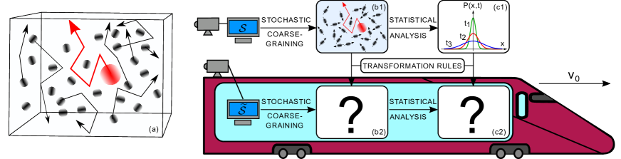
Figure 1: Pictorial representation of the setup: a system of $N$ heat bath particles (black) and one tracer (red) is observed from two different reference frames $\mathcal{S}$ and $\widetilde{\mathcal{S}}$. While $\mathcal{S}$ is at rest, $\widetilde{\mathcal{S}}$ is moving with velocity $v_{0}$ with respect to $\mathcal{S}$. We consider three different levels of description of the original system: (a) The microscopic system of $N+1$ particles is described by deterministic equations of motion leading to trajectories fully specified by the initial conditions. (b1) Alternatively, one can provide a stochastic coarse-grained model of the tracer dynamics in terms of effective dissipative friction forces and random collisions with the $N$ bath particles (arrowed spheres), which account for their original microscopic interactions with the probe. (c1) Finally, the system can be studied in terms of its position and velocity statistics, whose distributions are uniquely determined by either experimental measurements or by a prescribed stochastic model. While the relationship between the dynamical evolutions in $\mathcal{S}$ and $\tilde{\mathcal{S}}$ for (a) is specified by Galilean transformations of the position and velocity degrees of freedoms, here we derive the corresponding relationships for (b1) $\leftrightarrow$ (b2) and (c1) $\leftrightarrow$ (c2) yielding what we call weak Galilean invariance.

Classical mechanics is built upon the two intimately related concepts of inertial reference frames and Galilean invariance (GI) arnol2013mathematical . The former are coordinate systems where a freely moving particle (i.e., in the absence of external forces) either is at rest or exhibits uniform rectilinear motion. The latter principle states that in different inertial frames the equations of motion of closed systems, i.e., including all their interacting constituents, are invariant with respect to Galilean transformations (GTs). These are in general affine transformations, that preserve both time intervals and distances between simultaneous events arnol2013mathematical . For systems whose dynamical evolution can be fully characterized by microscopic deterministic models, GI plays a fundamental constitutive role, manifest in the constraints that it naturally imposes on the functional form of Newton’s equation. However, a large variety of complex systems in science and nature are not modelled on a microscopic level with Newtonian equations of motion, but rather on a mesoscopic level using, e.g., stochastic Langevin equations or Fokker-Planck diffusion equations to capture the coarse-grained effects of microscopic interactions as friction and noise on the relevant degrees of freedom. The applications of such equations and their variants are vast throughout the sciences Van-Kampen:2011aa ; Gardiner:2010aa ; Kalmykov:2012aa .

Coarse-grained diffusive models are particularly relevant to describe anomalous transport phenomena, where stochasticity arises due to complex multi-particle interactions, whose precise form is usually unknown. While for normal diffusion due to Brownian motion the mean-square displacement (MSD) of an ensemble of particles with positions $X(t)$ at time $t$ grows linearly in the long-time limit, $\langle X^{2}\rangle\sim t^{\beta}$ with $\beta=1$, for anomalous diffusion it scales non-linearly with $\beta\neq 1$. Anomalous dynamics has been observed experimentally for a wide range of physical processes like particle transport in plasmas, molecular diffusion in nanopores and charge transport in amorphous semiconductors metzler2000random ; mekl04 ; klages2008anomalous , that was first theoretically described in scher1973stochastic ; scher1975anomalous based on the Continuous time random walk (CTRW) montroll1965random . Likewise, anomalous diffusion has been later found for biological motion HoFr13 ; Dieterich:2008aa ; Harris2012 , and even human movement Brockmann:2006aa . Recently, it has been established as an ubiquitous characteristic of cellular processes on a molecular level Bressloff:2013aa . Here, anomalous diffusion is observed, e.g., in neuronal messenger ribonucleoprotein transport Song2018 , in protein structural fluctuations Hu:2015aa , and in the intracellular transport of S. cerevisiae mitochondria senning2010actin , chromosomal loci of E. coli cells Weber2010 ; Javer2014 , engulfed microspheres Caspi2000 , lipid and insulin granules Jeon2011 ; tabei2013intracellular . However, because of the intrinsic difficulties in assessing the details of the microscopic interactions in experiments, theoretical models for such anomalous processes cannot be typically derived from first principles and are usually formulated on mostly phenomenological grounds. In fact, a wealth of diffusive models has been suggested in the literature, which rely on spatiotemporal memory effects and non-Gaussian power-law statistics of various observables metzler2000random ; klages2008anomalous ; zaburdaev2015levy ; Meroz:2015aa . Unfortunately so far there is no fundamental rule available that could be employed to verify the physical consistency of such stochastic models a priori. To distinguish between different models it remains only the comparison with experimental data that is often imprecise due to limited sample sizes.

Here, we show that GI can provide precisely such a constitutive principle. Even though the fundamental role of GI seemingly breaks down for stochastic diffusive models due to the presence of friction sekimoto2010stochastic , they are nevertheless constrained by a weak form of GI in order to be physically consistent in different inertial frames. The weak GI rules derived below thus represent a general selection principle for stochastic coarse-grained models. Previously, the consequences of GI in the context of statistical mechanics were first explored for fluid dynamics, where it establishes specific relations between critical exponents of the characteristic parameters entering the derivation of the Navier-Stokes equation forster1977large (although this result has been challenged berera2007gauge ). The problem carries over to the famous KPZ equation kardar1986dynamic whose GI is equally debated wio2010kpz . Whether or not these statistical equations feature GI has important practical implications for the modelling of, e.g., fluid flows berera2007gauge and nonlinear biological growth escudero2010 . Specifically, in molecular dynamics simulations of fluids employing stochastic Langevin thermostats it was found that Langevin dynamics breaks GI by violating global momentum conservation, which makes it unsuitable to simulate hydrodynamic phenomena duenweg1993 . Curing this deficiency led to novel GI algorithms, most notably dissipative particle dynamics, now widely used to simulate soft matter systems and simple liquids hoogerbrugge1992simulating ; soddemann2003 ; pastorino2015 .

The basic setup of our problem is represented in Fig. 1: here $\mathcal{S}$ and $\widetilde{\mathcal{S}}$ are two inertial reference frames, where $\mathcal{S}$ is the laboratory frame at rest while $\widetilde{\mathcal{S}}$ is moving with uniform velocity $v_{0}$ with respect to $\mathcal{S}$. The GTs connecting the coordinates in the two frames are given by

$$\widetilde{x}=x-v_{0}t\>,\qquad\qquad\widetilde{v}=v-v_{0}\>,$$ (1)

where, for simplicity, we focus on the one dimensional case. (1) is the phase space version of the classical GTs assuming an absolute time arnol2013mathematical . A classical system of $N+1$ interacting particles is described by the Hamiltonian function

$$H(x_{1},v_{1};\ldots;x_{N+1},v_{N+1})=\\ \sum_{i}\frac{m_{i}}{2}v_{i}^{2}(t)+\sum_{i<j}U(x_{i}(t),x_{j}(t))\>,$$ (2)

where $x_{i}$, $v_{i}$ are the position-velocity coordinates of the $i$-th particle in the reference frame $\mathcal{S}$ and $U$ is the interaction potential satisfying some mild regularity conditions. Its dynamics is specified by Hamilton’s equations

$$\dot{x}_{i}(t)=v_{i}(t)\>,\quad m_{i}\dot{v}_{i}(t)=-\frac{\partial}{\partial x_{i}}\sum_{i<j}U(x_{i}(t),x_{j}(t))\>.$$ (3)

Transforming the coordinates to the reference frame $\widetilde{\mathcal{S}}$ via Eqs. (1), we see that $\dot{\widetilde{x}}_{i}(t)=\widetilde{v}_{i}(t)$ and $m_{i}\dot{\widetilde{v}}_{i}(t)=-\frac{\partial}{\partial\widetilde{x}_{i}}\sum_{i<j}U(\widetilde{x}_{i}(t),\widetilde{x}_{j}(t))$ if $U$ depends only on the relative difference between the particles’ positions, i.e., $U(x_{i}(t),x_{j}(t))=U(x_{i}(t)-x_{j}(t))$, because in this case $\widetilde{x}_{i}(t)-\widetilde{x}_{j}(t)=x_{i}(t)-x_{j}(t)$. We thus recover Newton’s equations of motion satisfying his Third Law, which are identical in both reference frames, i.e., they satisfy GI. Our goal is now to derive coarse-grained dynamics from systems described by Eqs. (3), where some of the microscopic degrees of freedom have been eliminated, and to characterize their statistics on such a mesoscopic level in both frames $\mathcal{S}$, $\widetilde{\mathcal{S}}$ (see Fig. 1).

The transition from Eqs. (3) to an effective description in the form of a stochastic diffusion equation can be made quantitatively precise for the specific scenario where one of the particles, for simplicity let it be the $(N+1)$-th, is a tagged (tracer) particle of mass $m_{N+1}=M$, that interacts with the remaining particles of equal mass $m_{j}=m$ via an harmonic potential of coupling strength $m\omega^{2}_{j}$, thus defining the environment as a heat bath, i.e., $U(X,x_{j})\to\sum_{j=1}^{N}m\omega_{j}^{2}[X(t)-x_{j}(t)]^{2}/2$. Conversely, interactions between different bath particles are switched off. This is a Galilean invariant version of the classical Kac-Zwanzig model zwanzig1973nonlinear , whose relevance has been recently addressed deBacco2014 . Denoting by $(X(t),V(t))$ and $(x_{j}(t),v_{j}(t)),\,j\!=\!1,...,N$ the position and velocity variables of the tracer and heat bath particles, respectively, in the frame $\mathcal{S}$, their Hamilton’s equations become: $M\ddot{X}(t)=\sum_{j=1}^{N}m\omega_{j}^{2}\left[x_{j}(t)-X(t)\right]$ and $m\ddot{x}_{j}(t)=-m\omega_{j}^{2}\left[x_{j}(t)-X(t)\right]$. These equations specify the time evolution of all $N+1$ particles of the system (arrows in the box of Fig. 1a) in $\mathcal{S}$ once the initial conditions are prescribed, which we take as $(X(0),V(0))=(0,0)$ and $(x_{j}(0),v_{j}(0))=(x_{j0},v_{j0})$, without loss of generality. The great advantage of this model is that the effective dynamics for the tracer can be derived by integrating out the bath degrees of freedom. This yields zwanzig1973nonlinear

$$M\ddot{X}(t)=-\int_{0}^{t}\Omega(t-t^{\prime})\dot{X}(t^{\prime})\mathop{}\!\mathrm{d}t^{\prime}+\xi(t)\>,$$ (4)

where the memory kernel $\Omega$ and what later on will become the “noise” $\xi$ in Langevin dynamics are exactly zwanzig1973nonlinear

$$\Omega(t) =\sum_{j=1}^{N}\omega_{j}^{2}\cos{(\omega_{j}t)}\>,$$ (5)

$$\xi(t) =\sum_{j=1}^{N}\omega_{j}v_{j0}\sin{(\omega_{j}t)}+\sum_{j=1}^{N}\omega_{j}^{2}x_{j0}\cos{(\omega_{j}t)}\>.$$ (6)

As can be seen from (6), $\xi$ depends explicitly on the initial conditions of the bath particles, which are related to those in $\widetilde{\mathcal{S}}$ by $\widetilde{x}_{j0}=x_{j0}$, $\widetilde{v}_{j0}=v_{j0}-v_{0}$ and $\widetilde{X}(0)=0$, $\widetilde{V}(0)=-v_{0}$. Since everything is exact, the dynamics in $\widetilde{\mathcal{S}}$ follows by applying the GTs of Eqs. (1) to Eqs. (4–6). $\Omega$ is unchanged under the transformation, but (6) is changed due to the GTs of the initial velocities of the bath particles. If we call $\widetilde{\xi}$ the noise term in the transformed frame, i.e., (6) in $\sim$ variables, the two noises are related by

$$\xi(t)=\widetilde{\xi}(t)+v_{0}\sum_{j=1}^{N}\omega_{j}\sin{(\omega_{j}t)}=\widetilde{\xi}(t)+v_{0}\int_{0}^{t}\Omega(t^{\prime})\mathop{}\!\mathrm{d}t^{\prime}\>.$$ (7)

Overall, the deterministic coarse-grained equation of the tracer in $\widetilde{\mathcal{S}}$ is then just (4) in $\sim$ variables

$$M\ddot{\widetilde{X}}(t) =-\int_{0}^{t}\Omega(t-t^{\prime})\dot{\widetilde{X}}(t^{\prime})\mathop{}\!\mathrm{d}t^{\prime}+\widetilde{\xi}(t)$$ (8)

$$=-\int_{0}^{t}\Omega(t-t^{\prime})(\dot{\widetilde{X}}(t^{\prime})+v_{0})\mathop{}\!\mathrm{d}t^{\prime}+\xi(t),$$ (9)

using (7). The deterministic effective equation of motion for the tracer thus maintains the GI of the original microscopic dynamics even after projecting out the degrees of freedom of the bath particles. For deriving stochastic Langevin dynamics the next step is to simplify this coarse-grained description by specifying $\xi(t)$ as a random force instead of the deterministic force (6). On the Langevin level, the dynamics of the tracer then effectively originates from both dissipative friction forces and random collisions with the bath particles, accounting for their original microscopic interactions with the probe. The statistics of $\xi(t)$ is specified by the distribution of $x_{j0}$, $v_{j0}$. Assuming that the heat bath is at equilibrium in $\mathcal{S}$, the velocity distribution is Maxwellian at the temperature of the system $T$ implying $\left<\xi(t)\right>\!=\!0$ and $\left<\xi(t_{1})\xi(t_{2})\right>=k_{B}T\Omega(|t_{1}-t_{2}|)$ zwanzig1973nonlinear . Consequently, the fluctuation-dissipation relation holds kubo1966fluctuation . Equation (4) then defines a generalized Langevin equation (LE) in $\mathcal{S}$. Crucially, the notion of thermal equilibrium is not frame invariant such that the stochastic coarse-graining is not possible directly for (8). Specifying the properties of the random force that way per se singles out a reference frame and thus inevitably breaks GI, because according to (7) the noise $\tilde{\xi}$ acquires a different statistics than $\xi$. However, after having specified $\xi$ via the equilibrium assumption in $\mathcal{S}$, (9) is still valid. Eqs. (4,9) then both represent the same microscopic dynamics in two different inertial frames. We see that (9) contains an additional drift term, which could be obtained directly from (4) by performing a GT on the coordinates of its deterministic part only while leaving the noise term unchanged.

The transformation rules of the stochastic equations of motion imply that the resulting position-velocity processes ($X$, $V$) and ($\widetilde{X}$, $\widetilde{V}$) are related via a GT, even in the presence of stochasticity, which can be shown by explicitly solving these equations (4,9), while correctly accounting for the different initial conditions in the two frames (Appendix A). Consequently, also the probability density functions (PDFs) for position and velocity in different inertial frames can be related to each other directly. Including the position coordinates as $\dot{X}(t)=V(t)$ and ${\dot{\widetilde{X}\mkern 3.5mu}\mkern-3.5mu}{}(t)=\widetilde{V}(t)$ we have for underdamped dynamics the PDF transformation rule

$$P(x,v,t) = \left<\delta(x-X(t))\delta(v-V(t))\right>$$ (10)

$$= \left<\delta(x-\widetilde{X}(t)-v_{0}t)\delta(v-\widetilde{V}(t)-v_{0})\right>$$

$$= \widetilde{P}(x-v_{0}t,v-v_{0},t)\>,$$

since the expected value in both inertial frames is over the fluctuations of the same heat bath defined in $\mathcal{S}$. In terms of its Fourier-Laplace transform (from now on denoted by different independent variables according to $(x,v,t)\to(k,p,\lambda)$) the connection is $P(k,p,\lambda)=e^{-ipv_{0}}\widetilde{P}(k,p,\lambda-ikv_{0})$. For overdamped dynamics the respective results are $P(x,t)=\widetilde{P}(x-v_{0}t,t)$ and in Fourier-Laplace space

$$P(k,\lambda)=\widetilde{P}(k,\lambda-iv_{0}k)\>.$$ (11)

Their evolution equations can also be shown to transform via a GT on their independent variables (Appendix B).

So far we have shown that a stochastic coarse-grained description inherently violates GI. Nevertheless, (7)) characterizes the stochastic dynamics in all different Galilean frames uniquely as follows: (i) Stochastic equations of motion transform via a GT on their position and velocity processes only; consequently, (ii) Fokker-Planck (FP) and Klein-Kramers equations also transform via a GT on their independent variables, and (iii) PDFs transform as in Eqs. (10, 11). The validity of the properties (i)–(iii) is non-trivial and needs in principle to be shown for any specific stochastic model at hand following a coarse-graining procedure. These three Galilean transformation rules for coarse-grained stochastic dynamics and its statistical counterparts yield what we call weak GI: apart from a shift of $v_{0}$ or $v_{0}t$ for velocity and position variables, respectively, the corresponding PDFs in $\widetilde{\mathcal{S}}$ remain unchanged compared to the ones in $\mathcal{S}$. It is important to distinguish these weak GI rules from conventional microscopic GI. In systems satisfying the latter, the equations of motion are strictly identical in all inertial frames, while their stochastic coarse-grained equivalents are different.

Clearly, all processes described by the generalized LE (4) satisfy (i)–(iii), which includes normal diffusive processes. In this case the FP equation in $\widetilde{\mathcal{S}}$ is the well-known advection-diffusion equation. (4)) also models anomalous diffusion if one uses for $\Omega$ a power law kernel in time kupferman2004fractional , which highlights that these properties are preserved in the anomalous regime. However, in modelling anomalous diffusion a large variety of processes are used for which a similarly rigorous coarse-graining procedure is not available metzler2000random ; klages2008anomalous ; zaburdaev2015levy ; KlSo11 . While the accurate determination of an underlying anomalous stochastic process ultimately relies on the comparison of statistical quantities beyond the MSD with experimental data HoFr13 , we propose that weak GI can serve as an important criterion to assess the physical consistency of stochastic models from a purely theoretical first principles perspective.

In fact, we verified the validity of our conjecture for several other stochastic models generating both sub- and superdiffusion, that are commonly used in the literature, such as Fractional and Scaled Brownian motion mandelbrot1968fractional ; lim2002self ; hofling2013anomalous , the Fractional LE Lutz2001 ; lim2002self ; hofling2013anomalous , Lévy flights hughes1981random ; fogedby1992fluctuations ; chechkin2006fundamentals , Lévy walks shlesinger1987levy ; sokolov2003towards ; zaburdaev2015levy ; fedotov2016single , and the CTRW montroll1965random ; fogedby1994langevin ; metzler2000random . An overview is presented in Appendix Table A1, where for simplicity we only demonstrate the validity of property (ii) (details of the calculations are discussed in Appendix B). Remarkably, apart from the CTRW, all representations exhibit weak GI, i.e., applying a GT to the given Langevin or FP description yields solutions in agreement with Eqs. (10, 11). For Fractional Brownian motion, Scaled Brownian motion, and the Fractional LE (as a special case of the generalized LE), this result can be proven based on the Gaussian nature of the process. For Lévy flights it is a direct consequence of the Lévy-Khintchine representation of Lévy processes cont1975financial . In these examples, the Langevin dynamics can be expressed in terms of an additive noise process and thus the transformation into frame $\widetilde{\mathcal{S}}$ by GT is unproblematic leading to an advective term $v_{0}\partial/\partial x$ as for normal diffusion. Even though such a simple structure does not apply to Lévy walks, surprisingly the same consistency is satisfied, as can be checked by imposing a GT onto the respective FP equation fedotov2016single and verifying that the solutions in each frame are related by (11). The FP equation in $\widetilde{\mathcal{S}}$ describes a Lévy walk with asymmetric velocity jumps switching between $-v_{0}+u$ and $-v_{0}-u$, where $\pm u$ is the velocity in $\mathcal{S}$, which clearly is physically correct.

We now clarify the situation for the CTRW, a model that has huge applications across all branches of the sciences metzler2000random ; mekl04 ; klages2008anomalous ; KlSo11 . In the overdamped regime the PDF $P$ of a CTRW in the frame $\mathcal{S}$ is the solution of the diffusion equation magdziarz2009langevin ; cairoli2015anomalous

$$\frac{\partial}{\partial t}P(x,t)=\mathcal{L}\mathbb{D}_{t}P(x,t),\qquad\mathcal{L}=\sigma\frac{\partial^{2}}{\partial x^{2}},$$ (12)

where $\sigma$ is a generalized diffusion constant and $\mathbb{D}_{t}$ is a non-local time operator defined as $\mathbb{D}_{t}P(x,t)=\frac{\partial}{\partial t}\int_{0}^{t}{\rm d}t^{\prime}K(t-t^{\prime})P(x,t^{\prime})$, which generalizes the Riemann-Liouville fractional differential operator to arbitrary waiting time distributions. The kernel $K$ is related to the so-called Laplace exponent $\Phi$ of the waiting time distribution by $K(\lambda)=\Phi(\lambda)^{-1}$ magdziarz2009langevin ; cairoli2015anomalous . Therefore, its Fourier-Laplace representation is $\mathbb{D}_{t}P(x,t)\to\lambda P(k,\lambda)/\Phi(\lambda)$. In the CTRW framework a constant drift can be incorporated by complementing the diffusion operator with $v_{0}\partial/\partial x$, which would suggest that the FP equation in $\widetilde{\mathcal{S}}$ is given by $\frac{\partial}{\partial t}\widetilde{P}=\left[v_{0}\frac{\partial}{\partial x}+\mathcal{L}\right]\mathbb{D}_{t}\widetilde{P}$. Alternatively, another time non-local FP equation was previously derived, in particular for $\Phi(\lambda)=\lambda^{\alpha}$ ($0<\alpha<1$) corresponding to Lévy stable distributed waiting times, by employing the transformation rule (11) and performing a Taylor expansion in the Fourier variable up to the lowest approximation order metzler1998anomalous ; metzler1999transport ; metzler2000random . This procedure leads to the equation: $\frac{\partial}{\partial t}\widetilde{P}=v_{0}\frac{\partial}{\partial x}\widetilde{P}+\mathcal{L}\mathbb{D}_{t}\widetilde{P}$.

However, both equations are not correct representations of microscopic dynamics in view of the rules (i)–(iii) yielding weak GI. In fact, the former does not satisfy the general rule (11) as becomes clear by solving it in Fourier-Laplace space. The same is true for the latter, whose solutions are even unphysical, as they do not satisfy the requirement of positivity of a PDF (Fig. 2a and Appendix C). Therefore, a simple transformation of the fractional diffusion equation obtained by arbitrarily adding an advective term $v_{0}\partial/\partial x$ as for the Gaussian models and Lévy flights (see Table S1) is not correct. Likewise, implementing GTs directly on the Langevin description of CTRWs in terms of subordination fogedby1994langevin ; cairoli2015anomalous ; cairoli2017timedep is problematic (see below).

Instead, the correct transformation of (12)) into the frame $\widetilde{S}$ can be derived straightforwardly in Fourier-Laplace space. Without loss of generality, we assume $P(x,0)=\delta(x)$. Thus, its transform is $\lambda P(k,\lambda)-1=-\sigma k^{2}[\lambda/\Phi(\lambda)]P(k,\lambda)$. Employing property (iii), the GT is then implemented by the variable transformation $\lambda\to\lambda+ikv_{0}$ and the transformation rule (11)) relating $P,\widetilde{P}$. This immediately leads to a FP equation including retardation effects

$$\frac{\partial}{\partial t}\widetilde{P}(x,t)=v_{0}\frac{\partial}{\partial x}\widetilde{P}(x,t)+\mathcal{L}\mathcal{D}_{t}^{(v_{0})}\widetilde{P}(x,t)\>,$$ (13)

where the operator $\mathcal{D}^{(v_{0})}_{t}$ is the fractional substantial derivative sokolov2003towards ; Friedrich2006Anomalous ; cairoli2015anomalous

$$\mathcal{D}^{(v_{0})}_{t}\widetilde{P}(x,t)=\left[\frac{\partial}{\partial t}-v_{0}\frac{\partial}{\partial x}\right]\int_{0}^{t}{\rm d}t^{\prime}K(t-t^{\prime})\widetilde{P}(x+v_{0}(t-t^{\prime}),t^{\prime})$$ (14)

which has Fourier-Laplace representation $\mathcal{D}^{(v_{0})}_{t}\widetilde{P}(x,t)\to(\lambda+iv_{0}k)\widetilde{P}(k,\lambda)/\Phi(\lambda+iv_{0}k)$. Setting $v_{0}\!=\!0$ recovers (12).

To further support our result, we also derive (13) directly in $(x,t)$-space. This requires a careful analysis due to the non-local character of the operator $\mathbb{D}_{t}$. On the one hand, the lhs of (12) and the time derivative in front of $\mathbb{D}_{t}$ transform with the substitution $\partial/\partial t\to\partial/\partial t-v_{0}\partial/\partial x$ (chain rule applied to Eqs. (1)). On the other hand, recalling the explicit definition of a PDF in terms of probability (denoted as $\mathds{P}$) of events (denoted as $\{\cdot\}$), the integrand PDF is defined as $P(x,t^{\prime})=\mathds{P}(\{x\leq Y(t^{\prime})\leq x+\mathop{}\!\mathrm{d}x\})$, where $Y(t)$ denotes the position of the CTRW. According to property (i), $Y(t^{\prime})$ becomes $\widetilde{Y}(t^{\prime})+v_{0}t^{\prime}$ in the comoving frame $\widetilde{\mathcal{S}}$, while the measured position $x$ transforms at the later time $t$ in agreement with the lhs of the equation, i.e., $x\!\to\!x+v_{0}t$. Therefore $P(x,t^{\prime})=\mathds{P}(\{x+v_{0}(t-t^{\prime})\leq\widetilde{Y}(t^{\prime})\leq x+v_{0}(t-t^{\prime})+\mathop{}\!\mathrm{d}x\})=\widetilde{P}(x+v_{0}(t-t^{\prime}),t^{\prime})$. Note that $\mathop{}\!\mathrm{d}x$ is invariant because the shift cancels out. Combining these arguments yields (13). The fractional substantial derivative in (14) highlights the existence of a space-time coupling, which is absent in the frame $\mathcal{S}$ but is naturally required: let $y$ be the position of the CTRW in $\mathcal{S}$ after its last jump occurred at time $t$, and $\tau$, $\Delta y$ respectively the waiting time to the next jump and its length. In $\mathcal{S}$ its position at time $t+\tau$ is then $y+\Delta y$. In $\widetilde{\mathcal{S}}$ this is $y-v_{0}\tau+\Delta y$ ((1), left). Thus, the final position in $\widetilde{\mathcal{S}}$ depends on both the jump amplitude $\Delta y$ and the waiting time $\tau$. Interestingly, a similar coupling is constitutive of the Lévy walk model zaburdaev2015levy , which explains why it satisfies weak GI.

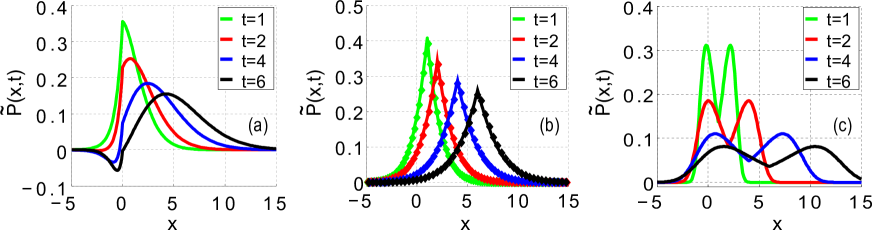
Figure 2: Position distribution in the comoving frame $\widetilde{\mathcal{S}}$. (a) Propagator of the Fokker-Planck equation $\frac{\partial}{\partial t}\widetilde{P}=v_{0}\frac{\partial}{\partial x}\widetilde{P}+\mathcal{L}\mathbb{D}_{t}\widetilde{P}$ suggested in metzler1998anomalous ; metzler1999transport ; metzler2000random instead of (13). The explicit expression for the propagator is given in Appendix C, Eq. (S47). This function not only violates weak GI, but also exhibits non-physical negative values. Here, $\Phi(\lambda)=\lambda^{\alpha}$ with $\alpha=0.5$, $v_{0}=-1$, $\sigma=1$, $x_{0}=0$. (b) PDF solution of (13) (Appendix D, Eq. (S68)) showing weak GI. Parameters are the same as for (a). We find perfect agreement with Monte-Carlo simulations of the Langevin equation $\dot{\widetilde{Y}}(t)=-v_{0}+\overline{\xi}(t)$ (colored markers). (c) PDF solution of (13) (Appendix D, Eq. (S68)) with $K(t)=t^{\alpha-1}/\Gamma(\alpha)$ and $\alpha$ analytically continued to yield superdiffusion at $\alpha=1.5$. Other parameters as for (b). Again, weak GI is observed.

What is now the corresponding Langevin dynamics of the anomalous diffusive process described by (13)? The key is to describe the CTRW directly in physical time rather than in the widely used subordination picture fogedby1994langevin ; cairoli2015anomalous ; cairoli2017timedep . In the physical time representation a CTRW in $\mathcal{S}$ is given as $\dot{Y}(t)=\overline{\xi}(t)$, where $\overline{\xi}$ is the derivative of a subordinated Brownian motion cairoli2015langevin . This is equivalently written as the formal definition $\overline{\xi}(t)=\int_{0}^{\infty}\xi(s)\delta(t-T(s))$, where $\xi$ is a white Gaussian noise with $\langle\xi(t)\rangle=0$ and $\langle\xi(t_{1})\xi(t_{2})\rangle=2\sigma\delta(t_{1}-t_{2})$, and $T$ is a strictly increasing Lévy process. Using this representation, we can calculate the characteristic functional $G$ of $\overline{\xi}$ for a general test function $u$ (Appendix D)

$$G[u(r)] =\left<\exp{\left[-\sigma\int_{0}^{\infty}[u(T(s))]^{2}\mathop{}\!\mathrm{d}s\right]}\right>,$$ (15)

where the brackets denote an average over the realizations of the process $T$. A GT can now be performed without problems leading to $\dot{\widetilde{Y}}(t)=-v_{0}+\overline{\xi}(t)$. Remarkably, employing functional techniques caceres1997generalized together with the result in (15), we can show that the FP equation for this process is precisely given by (13), thus completing the picture (Appendix D). The Langevin description in physical time highlights that to correctly implement the change of frame, the constant advective force exerted on the underlying random walk in the frame $\widetilde{S}$ needs to act at each time step, i.e., also during the trapping times. This simple physical scenario underlies the complicated space-time coupling manifest in the retardation of (13). Its modelling in terms of subordination thus inevitably couples the equations for the position and elapsed time processes, which makes any analytical treatment challenging (an example is discussed in Appendix E, where we derive (13) for the process $\widetilde{Y}$ using its representation in terms of coupled subordinated equations). Further using the characteristic functional of the noise $\overline{\xi}$ in (15) one can derive its analytical solution

$$\widetilde{P}(k,\lambda)=\frac{1}{\lambda+ikv_{0}}\left[1-\frac{\sigma k^{2}}{\Phi(\lambda+ikv_{0})+\sigma k^{2}}\right],$$ (16)

whose inverse Fourier-Laplace transform is plotted in Fig. 2b for the particular case of $T$ being a Lévy stable process of order $\alpha$ (Appendix D, Eq. (S68)). We observe the typical distribution of a force-free CTRW metzler2000random time-shifted with velocity $v_{0}$, in perfect agreement with numerical simulations of $\widetilde{Y}$.

Moreover, we find that $\widetilde{Y}$ can also generate a superdiffusive MSD thus providing a unified model for both sub- and superdiffusion. This surprising fact relies on the Langevin description in physical time and the equivalent characterization of $\overline{\xi}$ by means of its multipoint correlation functions cairoli2015langevin . In particular, its FP equation is still (13), which can be derived by a generalization of Novikov’s theorem via functional methods novikov1965functionals ; hanggi1978correlation (Appendix F), and the resulting PDF satisfies weak GI. In Fig. 2c we plot its propagator for $K(t)=t^{\alpha-1}/\Gamma(\alpha)$, now for $1<\alpha<2$ (Appendix D, Eq. (S68), analytically continued in $\alpha$). For $v_{0}=0$, this PDF was discussed in metzler2000accelerating .

In summary, using a Galilean invariant version of the paradigmatic Kac-Zwanzig model, we have derived the weak GI properties (i)–(iii) that need to be satisfied in order to consistently describe the same stochastic system in different inertial frames. While these properties hold for normal diffusion based on our analytical derivation, by employing these rules consistent anomalous diffusive models can be constructed for both sub- and superdiffusion, even though a precise coarse-graining procedure is missing for them. We demonstrated this by providing the missing representation for the important class of CTRW models, which shows that the correct form is not at all suggested from the representation in the rest frame. Moreover, the Langevin representation (i) discloses that in a comoving frame the heat bath leads generally to an additive flow field on the tracer particle irrespective of the details of the underlying coupling. Consequently, the definitions of work, heat and entropy production used within the recent theory of stochastic thermodynamics Seifert:2012aa have to be modified to account for the contribution of the external flow Speck:2008aa highlighting fundamental similarities between normal and anomalous diffusive systems, even though the stochastic thermodynamics of the latter is so far not well understood Chechkin:2012aa . Along these lines, connections between GI and the validity of fluctuation-dissipation relations on the one hand, and the celebrated fluctuation relations generalizing the second law of thermodynamics Seifert:2012aa on the other, have been suggested Chechkin:2012aa ; Dieterich:2015aa and need to be investigated further. But our most important statement is that ignoring our weak GI rules can easily lead to unphysical models, as exemplified by the CTRW with an ad hoc advective term (Fig. 2a). The consequences of our results are thus far-reaching. Weak GI is expected to constrain all mesoscopic diffusive models whose microscopic representation is expected to satisfy conventional GI. As such, it provides an important selection principle on stochastic models preceding comparison with data, which can guide modelling approaches throughout the physical, chemical, and biological sciences.

Stochastic model	Fokker-Planck/Klein-Kramers eq. in $\mathcal{S}$	Fokker-Planck/Klein-Kramers eq. in $\widetilde{\mathcal{S}}$
Normal diffusion (overdamped)	$\left[\frac{\partial}{\partial t}-\mathcal{L}\right]P=0\qquad$	$\left[\frac{\partial}{\partial t}-v_{0}\frac{\partial}{\partial x}-\mathcal{L}\right]\widetilde{P}=0$
Normal diffusion (underdamped)	$\left[\frac{\partial}{\partial t}+\frac{\partial}{\partial x}v-\frac{\partial}{\partial v}\gamma v-\gamma\sigma\frac{\partial^{2}}{\partial v^{2}}\right]P=0$	$\left[\frac{\partial}{\partial t}+\frac{\partial}{\partial x}v-\frac{\partial}{\partial v}\gamma(v+v_{0})-\gamma\sigma\frac{\partial^{2}}{\partial v^{2}}\right]\widetilde{P}=0$
Fractional/Scaled Brownian motion	$\left[\frac{\partial}{\partial t}-\beta t^{\beta-1}\mathcal{L}\right]P=0$	$\left[\frac{\partial}{\partial t}-v_{0}\frac{\partial}{\partial x}-\beta t^{\beta-1}\mathcal{L}\right]\widetilde{P}=0$
Generalized Langevin equation	$\left[\frac{\partial}{\partial t}+\frac{\partial}{\partial x}v-\frac{\partial}{\partial v}\Gamma(t)v\right]P$	$\left[\frac{\partial}{\partial t}+\frac{\partial}{\partial x}v-\frac{\partial}{\partial v}\Gamma(t)(v+v_{0})\right]\widetilde{P}$
	$\qquad=\left[\frac{\partial^{2}}{\partial v^{2}}\sigma\Gamma(t)+\frac{\partial^{2}}{\partial x\partial v}D_{xv}(t)\right]P$	$\qquad=\left[\frac{\partial^{2}}{\partial v^{2}}\sigma\Gamma(t)+\frac{\partial^{2}}{\partial x\partial v}D_{xv}(t)\right]\widetilde{P}$
Lévy flight	$\left[\frac{\partial}{\partial t}-\nabla^{\beta}\right]P=0$	$\left[\frac{\partial}{\partial t}-v_{0}\frac{\partial}{\partial x}-\nabla^{\beta}\right]\widetilde{P}=0$
Lévy walk	$\left[\left(\frac{\partial}{\partial t}+u\frac{\partial}{\partial x}\right)\left(\frac{\partial}{\partial t}-u\frac{\partial}{\partial x}\right)\right]P_{u}$	$\left[\left(\frac{\partial}{\partial t}+u_{+}\frac{\partial}{\partial x}\right)\left(\frac{\partial}{\partial t}+u_{-}\frac{\partial}{\partial x}\right)\right]\widetilde{P}_{u}$
	$\qquad=-\left[\frac{1}{2}\mathcal{D}_{t}^{(-u,u)}+\frac{1}{2}\mathcal{D}_{t}^{(u,-u)}\right]P_{u}$	$\qquad=-\left[\frac{1}{2}\mathcal{D}_{t}^{(u_{-},u_{+})}+\frac{1}{2}\mathcal{D}_{t}^{(u_{+},u_{-})}\right]\widetilde{P}_{u}$
Continuous time random walk	$\left[\frac{\partial}{\partial t}-\mathcal{L}\mathbb{D}_{t}\right]P=0$	?

Table 1: Overview of generic stochastic models for normal and anomalous diffusion. For simplicity, we show their representations in terms of generalized Fokker-Planck or Klein-Kramers equations and neglect the explicit dependencies of the distributions $P$, $\widetilde{P}$ on the sample variables. For all models, except the Continuous time random walk, property $\textit{i}i$ holds, i.e., their evolution equations in different inertial frames are related by a Galilean transformation of their independent variables. We define the diffusion operator $\mathcal{L}=\sigma\frac{\partial^{2}}{\partial x^{2}}$.

Appendix A Solution of the generalized Langevin equations in $\mathcal{S}$ and $\widetilde{\mathcal{S}}$

Let us consider the generalised LE in the laboratory frame $\mathcal{S}$:

$$\dot{X}(t) =V(t), M\dot{V}(t) =-\int_{0}^{t}\Omega(t-t^{\prime})V(t^{\prime})\mathop{}\!\mathrm{d}t^{\prime}+\xi(t).$$ (17)

The tracer trajectory $(X(t),V(t))$, with initial condition $(X_{0},V_{0})$ at time $t=0$, can be obtained exactly by Laplace transforming Eq. (17). For the position, this yields $\lambda X(\lambda)-X_{0}=V(\lambda)$, while for the velocity

$$V(\lambda)=\frac{MV_{0}}{M\lambda+\Omega(\lambda)}+\frac{\xi(\lambda)}{M\lambda+\Omega(\lambda)}.$$ (18)

Transforming back these equations in time space, we obtain $X(t)=X_{0}+\int_{0}^{t}V(t^{\prime})\mathop{}\!\mathrm{d}t^{\prime}$ and

$$V(t)=MV_{0}w(t)+\int_{0}^{t}w(t-t^{\prime})\xi(t^{\prime})\mathop{}\!\mathrm{d}t^{\prime},$$ (19)

where the function $w$ is defined in Laplace transform by

$$w(\lambda)=[M\lambda+\Omega(\lambda)]^{-1}.$$ (20)

We then consider the corresponding dynamics in the comoving frame $\widetilde{\mathcal{S}}$. These are described by

$$\dot{\widetilde{X}}(t) =\widetilde{V}(t), M\dot{\widetilde{V}}(t) =-\int_{0}^{t}\Omega(t-t^{\prime})[\widetilde{V}(t^{\prime})+v_{0}]\mathop{}\!\mathrm{d}t^{\prime}+\xi(t).$$ (21)

As before, we can derive the exact trajectory $(\widetilde{X}(t),\widetilde{V}(t))$ by taking the Laplace transform of Eqs. (21). This yields for the position $\lambda\widetilde{X}(\lambda)-\widetilde{X}_{0}=\widetilde{V}(\lambda)$ and for the velocity

$$\widetilde{V}(\lambda)=\frac{M\widetilde{V}_{0}}{M\lambda+\Omega(\lambda)}-\frac{v_{0}\Omega(\lambda)}{\lambda[M\lambda+\Omega(\lambda)]}+\frac{\xi(\lambda)}{M\lambda+\Omega(\lambda)},$$ (22)

where $\widetilde{X}_{0},\widetilde{V}_{0}$ are the initial condition in the transformed frame. Employing the relations: $\widetilde{V}_{0}=V_{0}-v_{0}$ and $\widetilde{X}_{0}=X_{0}$, that result from the Galilean transformation (GT) Eq. (1), we find

$$\widetilde{V}(\lambda) =\frac{M(V_{0}-v_{0})}{M\lambda+\Omega(\lambda)}-v_{0}\frac{\Omega(\lambda)}{\lambda[M\lambda+\Omega(\lambda)]}+\frac{\xi(\lambda)}{M\lambda+\Omega(\lambda)}$$

$$=\frac{MV_{0}}{M\lambda+\Omega(\lambda)}+\frac{\xi(\lambda)}{M\lambda+\Omega(\lambda)}-\frac{v_{0}}{\lambda}$$

$$=V(\lambda)-\frac{v_{0}}{\lambda}.$$ (23)

Substituting this equation into that of the position, we can write

$$\lambda\widetilde{X}(\lambda) =X_{0}+V(\lambda)-\frac{v_{0}}{\lambda}=\lambda X(\lambda)-\frac{v_{0}}{\lambda}.$$ (24)

Taking their inverse Laplace transforms yields: $\widetilde{V}(t)=V(t)-v_{0}$ and $\widetilde{X}(t)=X(t)-v_{0}t$. These transformation rules for $X,V$ directly provide Eq. (10).

Appendix B Analysis of weak Galilean invariance for several stochastic coarse-grained models

In this appendix, we study several different stochastic models mandelbrot1968fractional ; lim2002self ; hofling2013anomalous ; Lutz2001 ; shlesinger1987levy ; sokolov2003towards ; zaburdaev2015levy ; fedotov2016single ; montroll1965random ; fogedby1994langevin ; metzler2000random , that are widely used in the literature to model both normal and anomalous diffusion, in terms of weak Galilean invariance (GI). An overview is given in Table 1.

B.1 Overdamped Gaussian processes: fractional and scaled Brownian motion

General overdamped Gaussian processes are described in the laboratory frame $\mathcal{S}$ by the LE

$$\dot{X}(t)=\xi(t),$$ (25)

where $\xi(t)$ is a Gaussian coloured noise with $\left<\xi(t)\right>=0$ and two-point correlation function $\left<\xi(t)\xi(t^{\prime})\right>=C(t,t^{\prime})$. The time evolution of its position distribution $P(x,t)=\left<\delta(x-X(t))\right>$ is given by

$$\frac{\partial}{\partial t}P(x,t)=-\frac{\partial}{\partial x}\left\langle\xi(t)\delta(x-X(t))\right\rangle.$$ (26)

To get a closed equation for $P$, one needs to compute the averaged quantity in its right-hand side (rhs). For Gaussian noise, one employs Novikov’s theorem novikov1965functionals ; hanggi1978correlation , that yields

$$\left\langle\xi(t)\delta(x-X(t))\right\rangle \!=\!\int_{0}^{t}C(t,t^{\prime})\left\langle\frac{\delta[\delta(x-X(t))]}{\delta\xi\!\left(t^{\prime}\right)}\right\rangle\mathop{}\!\mathrm{d}t^{\prime}$$

$$=-\frac{\partial}{\partial x}\int_{0}^{t}C(t,t^{\prime})\left\langle\delta(x-X(t))\frac{\delta X(t)}{\delta\xi(t^{\prime})}\right\rangle\mathop{}\!\mathrm{d}t^{\prime}=-\frac{\partial}{\partial x}D(t)P(x,t),$$ (27)

where $\delta X(t)/\delta\xi(t^{\prime})=\Theta\!\left(t-t^{\prime}\right)$ and $D(t)=\int_{0}^{t}C(t,t^{\prime})\mathop{}\!\mathrm{d}t^{\prime}$. Substituting it in Eq. (26), we obtain

$$\frac{\partial}{\partial t}P(x,t)=\frac{\partial^{2}}{\partial x^{2}}D(t)P(x,t).$$ (28)

The previous argument holds for both stationary noises, whose correlation function depends only on the time difference, i.e., $C(t,t^{\prime})=C(|t-t^{\prime}|)$, and non-stationary ones. In the former case, an important example is the fractional Brownian motion; in the latter case, the scaled Brownian motion mandelbrot1968fractional ; lim2002self ; hofling2013anomalous . These processes are defined by setting the two-point correlation function equal to $C(|t-t^{\prime}|)=\beta(\beta-1)|t-t^{\prime}|^{\beta-2}$ and $C(t,t^{\prime})=\beta t^{\beta-1}\delta(t-t^{\prime})$ respectively with $0<\beta<2$ hofling2013anomalous , that yield the same diffusion coefficient $D(t)=\beta t^{\beta-1}$. Eq. (28) is easily solved by the Gaussian $P(x,t)=e^{-\frac{x^{2}}{4\Sigma(t)}}/\sqrt{4\pi\Sigma(t)}$, where $\Sigma(t)=\int_{0}^{t}D(t^{\prime})\mathop{}\!\mathrm{d}t^{\prime}$. Applying the GT Eq. 1, we obtain: $\widetilde{P}(x,t)=e^{-\frac{(x+v_{0}t)^{2}}{4\Sigma(t)}}/\sqrt{4\pi\Sigma(t)}$. This is easily shown to satisfy the FP equation:

$$\frac{\partial}{\partial t}\widetilde{P}(x,t)=\left[\frac{\partial}{\partial x}v_{0}+\frac{\partial^{2}}{\partial x^{2}}D(t)\right]\widetilde{P}(x,t),$$ (29)

that corresponds to the LE

$$\dot{\widetilde{X}}(t)=-v_{0}+\xi(t).$$ (30)

Therefore, the description of overdamped Gaussian processes satisfies properties $i\!-\!iii$ (main text), i.e., it exhibits weak GI.

B.2 Generalised Langevin equation

We write the generalised Langevin Eq. (4) as (we set $M=1$ without loss of generality)

$$\dot{X}(t) =V(t), \dot{V}(t) =-\int_{0}^{t}\Omega(t-t^{\prime})V(t^{\prime})\mathop{}\!\mathrm{d}t^{\prime}+\xi(t),$$ (31)

where $\Omega$ is a prescribed drag coefficient and the coloured Gaussian noise $\xi$ has the two point correlation function

$$\langle\xi(t)\xi(t^{\prime})\rangle=C(|t-t^{\prime}|)=\sigma\Omega(|t-t^{\prime}|),$$ (32)

with $\sigma=k_{B}T$ ($T$ is the temperature of the bath at equilibrium). Thus, it satisfies the fluctuation-dissipation relation kubo1966fluctuation . Relevant examples are (a) underdamped normal diffusion, for which $\Omega(t)=\gamma\delta(t)$ ($\gamma>0$), and (b) fractional LE Lutz2001 ; lim2002self ; hofling2013anomalous , for which $\Omega(t)=\gamma_{\alpha}t^{-\alpha}/\Gamma(1-\alpha),\,\,0\!<\!\alpha\!<\!1,\,\,\gamma_{\alpha}>0$. We call $X_{0}=X(0),V_{0}=V(0)$ the initial conditions. Eq. (31) has been widely discussed in the main text in terms of weak GI. In particular, the validity of the properties $i,iii$ has been discussed. Here, we show that also property $ii$ holds. First, we derive the Klein-Kramers equation for its joint position-velocity probability density function (PDF) in the laboratory frame $\mathcal{S}$ $P(x,v,t)=\langle\delta(x-X(t))\delta(v-V(t))\rangle$. Due to the Gaussian nature of $\xi$, and using the exact solution of the dynamics Eq. (19), the joint characteristic function is adelman1976fokker ; wang1999nonequilibrium

$$P(k,p,t)=\exp{\left\{i\langle X(t)\rangle k+i\langle V(t)\rangle p-\frac{1}{2}[\sigma^{2}_{xx}(t)k^{2}+2\sigma^{2}_{xv}(t)kp+\sigma^{2}_{vv}(t)p^{2}]\right\}},$$ (33)

where $\langle X(t)\rangle=V_{0}\overline{w}(t)+X_{0}$, $\langle V(t)\rangle=V_{0}w(t)$ and we defined the auxiliary function $\overline{w}(t)=\int_{0}^{t}w(t^{\prime})\mathop{}\!\mathrm{d}t^{\prime}$ and

$$\sigma^{2}_{xx}(t) =\sigma\left[2\int_{0}^{t}\overline{w}(t^{\prime})\mathop{}\!\mathrm{d}t^{\prime}-\overline{w}^{2}(t)\right], \sigma^{2}_{vv}(t) =\sigma[1-w^{2}(t)], \sigma^{2}_{xv}(t) =\sigma\overline{w}(t)[1-w(t)].$$ (34)

We take the following partial derivatives in $t,p$ (to ease notation we drop any explicit dependence of $P$ on its variables):

$$\frac{1}{P}\frac{\partial}{\partial t}P =iV_{0}[w(t)k+\dot{w}(t)p]-\frac{1}{2}\left[2\sigma^{2}_{xv}(t)k^{2}+2\frac{\mathop{}\!\mathrm{d}missing}{\mathop{}\!\mathrm{d}t}\sigma^{2}_{xv}(t)kp+\frac{\mathop{}\!\mathrm{d}missing}{\mathop{}\!\mathrm{d}t}\sigma^{2}_{vv}(t)p^{2}\right],$$ (35a)

$$\frac{1}{P}\frac{\partial}{\partial p}P =-\sigma^{2}_{vv}(t)p-\sigma^{2}_{xv}(t)k+iV_{0}w(t),$$ (35b)

where we further used the relation $\frac{\mathop{}\!\mathrm{d}missing}{\mathop{}\!\mathrm{d}t}\sigma_{xx}^{2}=2\sigma_{xv}^{2}$. Eliminating $V_{0}$, we derive the following equation:

$$\frac{1}{P}\frac{\partial}{\partial t}P =[k-\Gamma(t)p]\frac{1}{P}\frac{\partial}{\partial p}P-D_{vv}(t)p^{2}-D_{xv}(t)kp,$$ (36)

where the drag and diffusion coefficients $\Gamma,D_{vv},D_{xv}$ are defined as

$$\Gamma(t) =-\frac{\dot{w}(t)}{w(t)}, D_{vv}(t) =\sigma\Gamma(t), D_{xv}(t) =\sigma[-1+w(t)+\Gamma(t)\overline{w}(t)].$$ (37)

Taking its inverse Fourier transform yields:

$$\frac{\partial}{\partial t}P(x,v,t) =\left[-\frac{\partial}{\partial x}v+\frac{\partial}{\partial v}\Gamma(t)v+\frac{\partial^{2}}{\partial v^{2}}\sigma\Gamma(t)+\frac{\partial^{2}}{\partial x\partial v}D_{xv}(t)\right]P(x,v,t).$$ (38)

For example (a), we find $\Gamma(t)=\gamma$, $D_{xv}(t)=0$, thus yielding the ordinary Klein-Kramers equation:

$$\frac{\partial}{\partial t}P(x,v,t) =-\frac{\partial}{\partial x}vP(x,v,t)+\gamma\frac{\partial}{\partial v}\left[v+\sigma\frac{\partial}{\partial v}\right]P(x,v,t).$$ (39)

Let us now consider the generalized LE in the comoving frame $\widetilde{\mathcal{S}}$, i.e., Eq. (9) , which we write as

$$\dot{\widetilde{X}}(t) =\widetilde{V}(t), \dot{\widetilde{V}}(t) =-\int_{0}^{t}\Omega(t-t^{\prime})[\widetilde{V}(t^{\prime})+v_{0}]\mathop{}\!\mathrm{d}t^{\prime}+\xi(t).$$ (40)

We now apply the previous technique to compute its Klein-Kramers equation. Being related by the GT Eq. (1) , only their first moment changes to $\langle\widetilde{X}(t)\rangle=\langle X(t)\rangle-v_{0}t$, $\langle\widetilde{V}(t)\rangle=\langle V(t)\rangle-v_{0}$. Therefore, the joint characteristic function in $\widetilde{\mathcal{S}}$ is

$$\widetilde{P}(k,p,t)=\exp{\left\{i\langle X(t)\rangle k+i\langle V(t)\rangle p-ikv_{0}t-ipv_{0}-\frac{1}{2}[\sigma^{2}_{xx}(t)k^{2}+2\sigma^{2}_{xv}(t)kp+\sigma^{2}_{vv}(t)p^{2}]\right\}},$$ (41)

such that Eqs. (35a), (35b) changes to

$$\frac{1}{\widetilde{P}}\frac{\partial}{\partial t}\widetilde{P} =iV_{0}[w(t)k+\dot{w}(t)p]-ikv_{0}-\frac{1}{2}[2\sigma^{2}_{xv}(t)k^{2}+\dot{\sigma}^{2}_{xv}(t)kp+\dot{\sigma}^{2}_{vv}(t)p^{2}],$$ (42a)

$$\frac{1}{\widetilde{P}}\frac{\partial}{\partial p}\widetilde{P} =-\sigma^{2}_{vv}(t)p-\sigma^{2}_{xv}(t)k-iv_{0}+iV_{0}w(t).$$ (42b)

Elimination of the parameter $V_{0}$ yields

$$\frac{1}{\widetilde{P}}\frac{\partial}{\partial t}\widetilde{P} =[k-\Gamma(t)p]\frac{1}{\widetilde{P}}\frac{\partial}{\partial p}\widetilde{P}-ip\Gamma(t)v_{0}-D_{vv}(t)p^{2}-D_{xv}(t)kp,$$ (43)

whose Fourier inverse is given by

$$\frac{\partial}{\partial t}\widetilde{P}(x,v,t) =\left[-\frac{\partial}{\partial x}v+\frac{\partial}{\partial v}\Gamma(t)(v+v_{0})+\frac{\partial^{2}}{\partial v^{2}}\sigma\Gamma(t)+\frac{\partial^{2}}{\partial x\partial v}D_{xv}(t)\right]\widetilde{P}(x,v,t).$$ (44)

The special case (a) follows straightforwardly, i.e.,

$$\frac{\partial}{\partial t}\widetilde{P}(x,v,t) =-\frac{\partial}{\partial x}v\widetilde{P}(x,v,t)+\gamma\frac{\partial}{\partial v}\left[(v+v_{0})+\sigma\frac{\partial}{\partial v}\right]\widetilde{P}(x,v,t).$$ (45)

Clearly, Eqs. (38), (44) satisfy property $ii$.

B.3 Lévy walk

The Lévy walk model shlesinger1987levy ; sokolov2003towards ; zaburdaev2015levy ; fedotov2016single is a special class of the spatiotemporally coupled continuous-time random walk (CTRW) montroll1965random ; fogedby1994langevin ; metzler2000random . This is typically employed to model position mean-square displacement superdiffusive behaviour, and thus has been widely used to describe transport processes in, e.g., biological systems zaburdaev2015levy . Here, we study only the $1$-dim case. In the laboratory frame $\mathcal{S}$ a Lévy walk is mathematically obtained as follows: A particle moves with constant speed $u_{\pm}=\pm u$, where for later convenience we denote by $u_{\pm}$ its forward/backward velocity, for a random running time $\tau$ sampled by a prescribed distribution $\psi$, after which it randomly changes its direction of motion. The position distribution of a process $X$ performing this type of dynamics is described in terms of master equations, similar to those of the CTRW metzler2000random , but with a coupled transition probability $\phi(y,\tau)=\frac{1}{2}[\delta(y-u_{+}\tau)+\delta(y-u_{-}\tau)]\psi(\tau)=\frac{1}{2}\delta(|y|-u\tau)\psi(\tau)$, that relates the walker’s position $y$ to the running time $\tau$. The GT to the comoving frame $\widetilde{\mathcal{S}}$ expressed by Eq. (1) only changes the walker’s velocity as $u_{\pm}=\pm u-v_{0}$. This is shown easily by transforming $\phi$, which yields $\widetilde{\phi}(\widetilde{y},\tau)=\frac{1}{2}\delta(|\widetilde{y}+v_{0}\tau|-u\tau)\psi(\tau)=\frac{1}{2}[\delta(\widetilde{y}+(v_{0}-u)\tau)+\delta(\widetilde{y}+(v_{0}+u)\tau)]\psi(\tau)$. Thus, the microscopic dynamics of Lévy walks is Galilean invariant, and we expect its position distribution $P_{u}$ to correspondingly satisfy weak GI. First, we show that property $iii$ is satisfied. Remarkably, its position PDF can be obtained exactly in the laboratory frame zaburdaev2015levy . In fact, denoting $P_{0}(x)$ the initial distribution and $\Psi(t)=1-\int_{0}^{t}\psi(t^{\prime})\mathop{}\!\mathrm{d}t^{\prime}$ the probability of sampling a running time larger than $t$, $P_{u}$ is given by

$$P_{u}(k,\lambda)=\frac{[\Psi(\lambda-iuk)+\Psi(\lambda+iuk)]P_{0}(k)}{2-[\psi(\lambda+iuk)+\psi(\lambda-iuk)]}.$$ (46)

Identifying in the previous eq. left/right velocities $u_{\pm}$ and substituting for those in the comoving frame $\widetilde{\mathcal{S}}$, we obtain the PDF

$$\widetilde{P}_{u}(k,\lambda) =\frac{[\Psi(\lambda-iu_{+}k)+\Psi(\lambda-iu_{-}k)]P_{0}(k)}{2-[\psi(\lambda-iu_{+}k)+\psi(\lambda-iu_{-}k)]}$$

$$=\frac{[\Psi(\lambda+iv_{0}k-iuk)+\Psi(\lambda+iv_{0}k+iuk)]P_{0}(k)}{2-[\psi(\lambda+iv_{0}k-iuk)+\psi(\lambda+iv_{0}k+iuk)]}=P(k,\lambda+iv_{0}k),$$ (47)

highlighting that the property Eq. (11) holds for Lévy walks ($P$, $\widetilde{P}$ are related by the Laplace variable change $\lambda\to\lambda+iv_{0}k$).

Secondly, we show that property $ii$ also holds. A FP type equation has recently been proposed for Lévy walks, that has the form in the laboratory frame $\mathcal{S}$ fedotov2016single

$$\left[\frac{\partial^{2}}{\partial t^{2}}-u^{2}\frac{\partial^{2}}{\partial x^{2}}\right]P_{u}(x,t)=-\frac{1}{2}\left[\frac{\partial}{\partial t}-u\frac{\partial}{\partial x}\right]\int_{0}^{t}K(t^{\prime})P_{u}(x-ut^{\prime},t-t^{\prime})\mathop{}\!\mathrm{d}t^{\prime}-\frac{1}{2}\left[\frac{\partial}{\partial t}+u\frac{\partial}{\partial x}\right]\int_{0}^{t}K(t^{\prime})P_{u}(x+ut^{\prime},t-t^{\prime})\mathop{}\!\mathrm{d}t^{\prime},$$ (48)

with the memory kernel being defined as $K(\lambda)=\psi(\lambda)/\Psi(\lambda)$. It is easy to verify that Eq. (48) yields Eq. (46) in Fourier-Laplace space. This equation can be conveniently cast into the form

$$\left[\frac{\partial^{2}}{\partial t^{2}}-u^{2}\frac{\partial^{2}}{\partial x^{2}}+\frac{1}{2}\mathcal{D}_{t}^{(-u,u)}+\frac{1}{2}\mathcal{D}_{t}^{(u,-u)}\right]P_{u}(x,t)=0,$$ (49)

where $\mathcal{D}_{t}^{(v_{1},v_{2})}$ is the fractional operator

$$\mathcal{D}^{(v_{1},v_{2})}_{t}P_{u}(x,t)=\left[\frac{\partial}{\partial t}+v_{1}\frac{\partial}{\partial x}\right]\int_{0}^{t}K(t-t^{\prime})P_{u}(x-v_{2}(t-t^{\prime}),t^{\prime}){\rm d}t^{\prime},$$ (50)

with Fourier-Laplace representation $\mathcal{D}^{(v_{1},v_{2})}_{t}P_{u}(x,t)\to(\lambda-ikv_{1})K(\lambda-ikv_{2})P_{u}(k,\lambda)$. For $v_{1}=v_{2}=-v_{0}$, $\mathcal{D}^{(v_{1},v_{2})}_{t}$ recovers the fractional substantial derivative Eq. (14). Applying the GT Eq. (1) to $\mathcal{D}^{(v_{1},v_{2})}_{t}$ in Laplace space yields $(\lambda-ik(-v_{0}+v_{1}))K(\lambda-ik(-v_{0}+v_{2}))P_{u}(k,\lambda+ikv_{0})\to\mathcal{D}^{(-v_{0}+v_{1},-v_{0}+v_{2})}_{t}\widetilde{P}_{u}(x,t)$. Therefore, we obtain the FP equation in $\widetilde{\mathcal{S}}$

$$\left[\frac{\partial^{2}}{\partial t^{2}}-2v_{0}\frac{\partial}{\partial t}\frac{\partial}{\partial x}+(v_{0}^{2}-u^{2})\frac{\partial^{2}}{\partial x^{2}}+\frac{1}{2}\mathcal{D}_{t}^{(-v_{0}-u,-v_{0}+u)}+\frac{1}{2}\mathcal{D}_{t}^{(-v_{0}+u,-v_{0}-u)}\right]\widetilde{P}_{u}(x,t)=0,$$ (51)

that can be written more neatly as

$$\left[\left(\frac{\partial}{\partial t}+u_{+}\frac{\partial}{\partial x}\right)\left(\frac{\partial}{\partial t}+u_{-}\frac{\partial}{\partial x}\right)+\frac{1}{2}\mathcal{D}_{t}^{(u_{-},u_{+})}+\frac{1}{2}\mathcal{D}_{t}^{(u_{+},u_{-})}\right]\widetilde{P}_{u}(x,t)=0,$$ (52)

which is the correct evolution equation for the Lévy walk dynamics in the comoving frame $\widetilde{\mathcal{S}}$.

Appendix C Derivation of the propagator plotted in Fig. 2A

We consider the fractional equation

$$\frac{\partial}{\partial t}\widetilde{P}(x,t)=v_{0}\frac{\partial}{\partial x}\widetilde{P}(x,t)+\sigma\frac{\partial^{2}}{\partial x^{2}}\mathbb{D}_{t}\widetilde{P}(x,t),$$ (53)

where $\mathbb{D}_{t}$ is the Riemann-Liouville operator with Fourier-Laplace representation $\mathbb{D}_{t}\widetilde{P}(x,t)\to\lambda^{1-\alpha}\widetilde{P}(k,\lambda)$ ($0<\alpha<1$), that is plotted in Fig. 2a. Without loss of generality, we assume null initial condition. First, we solve Eq. (53) in Fourier-Laplace space:

$$\widetilde{P}(k,\lambda) =\frac{1}{\lambda^{\alpha^{\prime}}+b(k)\lambda^{\beta}+c(k)},$$ (54)

with the auxiliary parameters $\alpha^{\prime}=1$, $\beta=1-\alpha$, $b(k)=\sigma k^{2}$ and $c(k)=ikv_{0}$. Note that $\alpha^{\prime}>\beta$, $\forall\alpha\in(0,1)$. We then expand in series as podlubny1998fractional

$$\widetilde{P}(k,\lambda)=\frac{1}{c(k)}\frac{1}{1+\frac{\lambda^{\alpha^{\prime}}+b(k)\lambda^{\beta}}{c(k)}} =\frac{1}{c(k)}\frac{\lambda^{-\beta}c(k)}{\lambda^{\alpha^{\prime}-\beta}+b(k)}\frac{1}{1+\frac{\lambda^{-\beta}c(k)}{\lambda^{\alpha^{\prime}-\beta}+b(k)}}$$

$$=\frac{\lambda^{-\beta}}{\lambda^{\alpha^{\prime}-\beta}+b(k)}\sum_{n=0}^{\infty}(-1)^{n}\frac{\lambda^{-\beta\,n}[c(k)]^{n}}{[\lambda^{\alpha^{\prime}-\beta}+b(k)]^{n}}=\sum_{n=0}^{\infty}[-c(k)]^{n}\frac{\lambda^{-\beta-\beta\,n}}{[\lambda^{\alpha^{\prime}-\beta}+b(k)]^{n+1}}.$$ (55)

We can now make a term by term Laplace inverse transform of Eq. (55) by recalling the formula for the Laplace transform of the three-parameter Mittag-Leffler function given in Eq. (G14). Thus, $\widetilde{P}(k,t)$ is given as

$$\widetilde{P}(k,t) =\sum_{n=0}^{\infty}[-c(k)]^{n}t^{n}E^{1+n}_{\alpha,1+n}\left(-t^{\alpha}b(k)\right)=\sum_{n=0}^{\infty}(-iv_{0}t)^{n}k^{n}E^{1+n}_{\alpha,1+n}\left(-\sigma t^{\alpha}k^{2}\right).$$ (56)

We now need to make a term by term inverse Fourier transform of Eq. (56). To this aim, we first rewrite it in terms of Fox H-functions by using the corresponding property given in Eq. (G15).In our case, we obtain:

$$E^{1+n}_{\alpha,1+n}\left(-\sigma t^{\alpha}k^{2}\right)=\frac{1}{\Gamma(1+n)}H_{1,2}^{1,1}\left[\sigma t^{\alpha}k^{2}\left|\begin{array}[]{l}(-n,1)\\[2.84544pt] (0,1),(-n,\alpha)\end{array}\right.\right].$$ (57)

Using this formula, the Fourier inverse transform of $k^{n}E^{1+n}_{\alpha,1+n}\left(-\sigma t^{\alpha}k^{2}\right)$ is expressed by cosine and sine transforms of Fox H-functions, i.e., it is given by

$$\frac{1}{2\pi}\int_{-\infty}^{\infty}\cos{(kx)}k^{n}H_{1,2}^{1,1}\!\left[\sigma t^{\alpha}k^{2}\left|\begin{array}[]{l}(-n,1)\\[2.84544pt] (0,1),(-n,\alpha)\end{array}\right.\!\!\right]\mathop{}\!\mathrm{d}k-\frac{i}{2\pi}\int_{-\infty}^{\infty}\sin{(kx)}k^{n}H_{1,2}^{1,1}\left[\sigma t^{\alpha}k^{2}\left|\begin{array}[]{l}(-n,1)\\[2.84544pt] (0,1),(-n,\alpha)\end{array}\right.\right]\mathop{}\!\mathrm{d}k.$$ (58)

Let us first assume $x>0$. We remark that (a) the first/second integral in Eq. (58) is not null only for even/odd indices, i.e., for $n=2\nu$/$1+2\nu$, $\forall\nu\in\mathbb{N}_{0}$ respectively, due to the parity of the Fox H-function, and that (b) they are equal to twice the corresponding integral on the semi-half positive line, once not null. Thus, we can use the property of the H-function given in Eqs. (132) to compute these integrals:

$$\int_{0}^{\infty}\cos{(kx)}k^{2\nu}H_{1,2}^{1,1}\!\left[\sigma t^{\alpha}k^{2}\left|\begin{array}[]{l}(-2\nu,1)\\[2.84544pt] (0,1),(-2\nu,\alpha)\end{array}\right.\!\!\right]\mathop{}\!\mathrm{d}k =\frac{\sqrt{\pi}2^{2\nu}}{|x|^{1+2\nu}}H_{3,2}^{1,2}\!\left[\frac{4\sigma t^{\alpha}}{x^{2}}\left|\begin{array}[]{l}\left(\frac{1}{2}-\nu,1\right),(-2\nu,1),(-\nu,1)\\[2.84544pt] (0,1),(-2\nu,\alpha)\end{array}\right.\!\!\right],$$ (59e)

$$\int_{0}^{\infty}\sin{(kx)}k^{1+2\nu}H_{1,2}^{1,1}\!\left[\sigma t^{\alpha}k^{2}\left|\begin{array}[]{l}(-1-2\nu,1)\\[2.84544pt] (0,1),(-1-2\nu,\alpha)\end{array}\right.\!\!\right]\!\mathop{}\!\mathrm{d}k =\frac{\sqrt{\pi}2^{1+2\nu}}{|x|^{2+2\nu}}H_{3,2}^{1,2}\!\left[\frac{4\sigma t^{\alpha}}{x^{2}}\left|\begin{array}[]{l}\left(-\frac{1}{2}-\nu,1\right),(-1-2\nu,1),(-\nu,1)\\[2.84544pt] (0,1),(-1-2\nu,\alpha)\end{array}\right.\!\!\right].$$ (59j)

By using the further property in Eq. (130) we obtain:

$$H_{1,2}^{1,1}\left[\sigma t^{\alpha}k^{2}\left|\begin{array}[]{l}(-n,1)\\[2.84544pt] (0,1),(-n,\alpha)\end{array}\right.\right]\xrightarrow[\text{inverse}]{\text{Fourier}}\frac{1}{\sqrt{\pi}}\left\{\begin{array}[]{ll}\frac{2^{2\nu}}{|x|^{1+2\nu}}H_{2,3}^{2,1}\left[\frac{x^{2}}{4\sigma t^{\alpha}}\left|\begin{array}[]{l}(1,1),(1+2\nu,\alpha)\\[2.84544pt] \left(\frac{1}{2}+\nu,1\right),(1+2\nu,1),(1+\nu,1)\end{array}\right.\right]&\quad n=2\nu\vspace{0.2cm}\\ \frac{(-i)2^{1+2\nu}}{|x|^{2+2\nu}}H_{2,3}^{2,1}\left[\frac{x^{2}}{4\sigma t^{\alpha}}\left|\begin{array}[]{l}(1,1),(2+2\nu,\alpha)\\[2.84544pt] \left(\frac{3}{2}+\nu,1\right),(2+2\nu,1),(1+\nu,1)\end{array}\right.\right]&\quad n=1+2\nu\end{array}\right.$$ (60)

These results enable us to write Eq. (54) explicitly in $(x,t)$-space in terms of two infinite series of Fox H-functions (corresponding to the original series over odd and even indices):

$$\widetilde{P}(x,t)=\frac{1}{\sqrt{\pi}}\sum_{\nu=0}^{\infty}\frac{(-1)^{\nu}(v_{0}t)^{2\nu}}{(2\nu)!}\frac{2^{2\nu}}{|x|^{1+2\nu}}H_{2,3}^{2,1}\!\left[\frac{x^{2}}{4\sigma t^{\alpha}}\left|\begin{array}[]{l}(1,1),(1+2\nu,\alpha)\\[2.84544pt] \left(\frac{1}{2}+\nu,1\right),(1+2\nu,1),(1+\nu,1)\end{array}\right.\!\!\right]\\ +\!\frac{1}{\sqrt{\pi}}\sum_{\nu=0}^{\infty}\frac{(-1)^{1+\nu}(v_{0}t)^{1+2\nu}}{(1+2\nu)!}\frac{2^{1+2\nu}}{|x|^{2+2\nu}}H_{2,3}^{2,1}\!\left[\frac{x^{2}}{4\sigma t^{\alpha}}\left|\begin{array}[]{l}(1,1),(2+2\nu,\alpha)\\[2.84544pt] \left(\frac{3}{2}+\nu,1\right),(2+2\nu,1),(1+\nu,1)\end{array}\right.\!\!\right].$$ (61)

Finally, we can exploit Eq. (131) to absorb the $x$-dependent multiplicative factors into the Fox H-functions. For each term separately, we obtain:

$$\frac{2^{2\nu}}{|x|^{1+2\nu}}H_{2,3}^{2,1}\left[\frac{x^{2}}{4\sigma t^{\alpha}}\left|\begin{array}[]{l}(1,1),(1+2\nu,\alpha)\\[2.84544pt] \left(\frac{1}{2}+\nu,1\right),(1+2\nu,1),(1+\nu,1)\end{array}\right.\right] =\frac{(\sigma t^{\alpha})^{-\nu}}{\sqrt{4\sigma t^{\alpha}}}H_{2,3}^{2,1}\left[\frac{x^{2}}{4\sigma t^{\alpha}}\left|\begin{array}[]{l}\left(\frac{1}{2}-\nu,1\right),\left(1+2\nu-\alpha\left(\frac{1}{2}+\nu\right),\alpha\right)\\[2.84544pt] (0,1),\left(\frac{1}{2}+\nu,1\right),\left(\frac{1}{2},1\right)\end{array}\right.\right]$$ (62e)

$$\frac{2^{1+2\nu}}{|x|^{2+2\nu}}H_{2,3}^{2,1}\left[\frac{x^{2}}{4\sigma t^{\alpha}}\left|\begin{array}[]{l}(1,1),(2+2\nu,\alpha)\\[2.84544pt] \left(\frac{3}{2}+\nu,1\right),(2+2\nu,1),(1+\nu,1)\end{array}\right.\right] =\frac{(\sigma t^{\alpha})^{-\nu-1/2}}{\sqrt{4\sigma t^{\alpha}}}H_{2,3}^{2,1}\left[\frac{x^{2}}{4\sigma t^{\alpha}}\left|\begin{array}[]{l}(-\nu,1),(2+2\nu-\alpha(1+\nu),\alpha)\\[2.84544pt] \left(\frac{1}{2},1\right),\left(1+\nu,1\right),(0,1)\end{array}\right.\right].$$ (62j)

In the opposite case $x<0$ the second term in the rhs of Eq. (58) changes sign, so that the sum over odd indices in Eq. (61) has an opposite sign as well. If we take this into account and substitute Eqs. (62e), (62j) into Eq. (61), we obtain that $\widetilde{P}(x,t)$ is defined as an infinite series of Fox H-functions ($\forall x\neq 0$), i.e.,

$$\widetilde{P}(x,t)=\frac{1}{\sqrt{4\pi\sigma t^{\alpha}}}\left[\Theta(x)\sum_{n=0}^{\infty}\frac{(-1)^{n}}{n!}\left(\frac{v_{0}t}{\sqrt{\sigma t^{\alpha}}}\right)^{n}\overline{H}_{2,3}^{2,1}\left(\frac{x^{2}}{4\sigma t^{\alpha}};\alpha,n\right)+\Theta(-x)\sum_{n=0}^{\infty}\frac{1}{n!}\left(\frac{v_{0}t}{\sqrt{\sigma t^{\alpha}}}\right)^{n}\overline{H}_{2,3}^{2,1}\left(\frac{x^{2}}{4\sigma t^{\alpha}};\alpha,n\right)\right],$$ (63)

where the auxiliary function $\overline{H}_{2,3}^{2,1}\left(x;\alpha,n\right)$ is defined as

$$\overline{H}_{2,3}^{2,1}\!\left(x;\alpha,n\right) =\left\{\begin{array}[]{ll}(-1)^{\nu}H_{2,3}^{2,1}\!\left[x\left|\begin{array}[]{l}\left(\frac{1-2\nu}{2},1\right),\left(\frac{\left(2-\alpha\right)(1+2\nu)}{2},\alpha\right)\\[2.84544pt] (0,1),\left(\frac{1+2\nu}{2},1\right),\left(\frac{1}{2},1\right)\end{array}\right.\!\!\right]&\quad n=2\nu\vspace{0.1cm}\\ (-1)^{\nu}H_{2,3}^{2,1}\!\left[x\left|\begin{array}[]{l}\left(-\nu,1\right),\left((2-\alpha)(1+\nu),\alpha\right)\\[2.84544pt] \left(\frac{1}{2},1\right),\left(1+\nu,1\right),(0,1)\end{array}\right.\!\!\right]&\quad n=1+2\nu\end{array}\right.$$ (70)

The previous formula is valid for $x\neq 0$. Therefore, we need to specify the value of the PDF in this point. In this case, only the sum over even indices contributes to the PDF in Eq. (56) (the sine transform in Eq. (58) is, in fact, null) with coefficients defined by solving the correspondent integral of Fox function with Eqs. (120), (G11):

$$\int_{0}^{\infty}k^{2\nu}H_{1,1}^{1,2}\left[\sqrt{\sigma t^{\alpha}}|k|\left|\begin{array}[]{l}\left(-2\nu,\frac{1}{2}\right)\\[2.84544pt] \left(0,\frac{1}{2}\right),\left(-2\nu,\frac{\alpha}{2}\right)\end{array}\right.\right]\mathop{}\!\mathrm{d}k=\left(\frac{1}{\sqrt{\sigma t^{\alpha}}}\right)^{1+2\nu}\frac{\left[\Gamma\left(\frac{1}{2}+\nu\right)\right]^{2}}{\Gamma\left((1+2\nu)\left(1-\frac{\alpha}{2}\right)\right)}.$$ (71)

By substituting such coefficients into the series over even indices, we obtain:

$$\widetilde{P}(0,t) =\frac{1}{\sqrt{4\sigma t^{\alpha}}}\sum_{\nu=0}^{\infty}\frac{(-1)^{\nu}(2\nu)!}{4^{\nu}(\nu!)^{2}}\frac{1}{\Gamma\left(\left(1-\frac{\alpha}{2}\right)(1+2\nu)\right)}\left(\frac{v_{0}^{2}t^{2-\alpha}}{4\sigma}\right)^{\nu}$$

$$=\frac{1}{\sqrt{4\sigma t^{\alpha}}}E^{1/2}_{2-\alpha,(2-\alpha)/2}\left(-\frac{v_{0}^{2}t^{2-\alpha}}{4\sigma}\right).$$ (72)

Note that Eq. (63) is expressed as an expansion in the constant force field $v_{0}$, i.e., the velocity of the frame $\widetilde{\mathcal{S}}$. As a sanity check, we compute the zero-th order term, which must be equal to the solution in the frame $\mathcal{S}$, i.e., the position PDF of a force-free CTRW metzler2000random . This is confirmed below (note that the corresponding terms in the two series in Eq. (63) are equal):

$$\widetilde{P}(x,t) =\frac{1}{\sqrt{4\pi\sigma t^{\alpha}}}H_{2,3}^{2,1}\!\left[\frac{x^{2}}{4\sigma t^{\alpha}}\left|\begin{array}[]{l}\left(\frac{1}{2},1\right),\left(\frac{2-\alpha}{2},\alpha\right)\\[2.84544pt] \left(0,1\right),\left(\frac{1}{2},1\right),\left(\frac{1}{2},1\right)\end{array}\right.\!\!\right]=\frac{1}{\sqrt{4\pi\sigma t^{\alpha}}}H_{1,2}^{2,0}\!\left[\frac{x^{2}}{4\sigma t^{\alpha}}\left|\begin{array}[]{l}\left(\frac{2-\alpha}{2},\alpha\right)\\[2.84544pt] \left(0,1\right),\left(\frac{1}{2},1\right)\end{array}\right.\!\!\right].$$ (77)

Here, we used the property of the Fox H-function given in Eq. (123).

At last, we check the normalisation of the derived formula for $\widetilde{P}$, which is expected as $\widetilde{P}(k=0,\lambda)=1/\lambda$. Due to the different sign of the sums over odd indices, only those over even ones contribute to the normalization of the PDF. Due to the parity of the Fox H-function, the integral can be restricted to the semi-half positive line:

$$\int_{-\infty}^{\infty}\widetilde{P}(x,t)\mathop{}\!\mathrm{d}x=\frac{1}{\sqrt{\pi\sigma t^{\alpha}}}\sum_{\nu=0}^{\infty}\frac{(-1)^{\nu}}{(2\nu)!}\left(\frac{v_{0}t}{\sqrt{\sigma t^{\alpha}}}\right)^{2\nu}\int_{0}^{\infty}H_{2,3}^{2,1}\!\left[\frac{x^{2}}{4\sigma t^{\alpha}}\left|\begin{array}[]{l}\left(\frac{1-2\nu}{2},1\right),\left((2-\alpha)\left(\frac{1+2\nu}{2}\right),\alpha\right)\\[2.84544pt] \left(0,1\right),\left(\frac{1+2\nu}{2},1\right),\left(\frac{1}{2},1\right)\end{array}\right.\right]\mathop{}\!\mathrm{d}x.$$ (78)

We compute the integral of the Fox H-function by recalling Eqs. (129), (G11):

$$\int_{0}^{\infty}H_{2,3}^{2,1}\!\left[\frac{x^{2}}{4\sigma t^{\alpha}}\left|\begin{array}[]{l}\left(\frac{1-2\nu}{2},1\right),\left((2-\alpha)\left(\frac{1+2\nu}{2}\right),\alpha\right)\\[2.84544pt] \left(0,1\right),\left(\frac{1+2\nu}{2},1\right),\left(\frac{1}{2},1\right)\end{array}\right.\right]\mathop{}\!\mathrm{d}x =\sqrt{\sigma t^{\alpha}}\Theta(-1),$$ (81)

where the function $\Theta$ is defined in Eq. (120), which in this specific case is

$$\Theta(s)\! =\!\frac{\Gamma\!\left(\frac{s}{2}\right)\Gamma\!\left(\frac{1}{2}+\nu+\frac{1}{2}s\right)\Gamma\!\left(\frac{1}{2}-\frac{s}{2}+\nu\right)}{\Gamma\!\left(\frac{1}{2}-\frac{1}{2}s\right)\Gamma\!\left((2-\alpha)\left(\frac{1+2\nu}{2}\right)+\frac{\alpha}{2}s\right)}\!=\!\frac{\Gamma\!\left(\frac{s}{2}\right)\Gamma\!\left(\frac{1}{2}+\nu+\frac{1}{2}s\right)}{\Gamma\!\left((2-\alpha)\left(\frac{1+2\nu}{2}\right)+\frac{\alpha}{2}s\right)}\prod_{i=0}^{\nu-1}\left(\frac{1}{2}-\frac{s}{2}+i\right).$$ (82)

For $s\!=\!-1$ all terms, except that for $\nu=0$, which is equal to $\sqrt{\pi}$, cancel out. Eq. (81) is then equal to $\sqrt{\pi\sigma t^{\alpha}}$, i.e., the PDF is correctly normalised.

Appendix D Derivation of the characteristic functional of the noise $\overline{\xi}$

The noise $\overline{\xi}$ can be formally defined as cairoli2015langevin

$$\overline{\xi}(t)=\int_{0}^{\infty}\xi(s)\delta(t-T(s))\mathop{}\!\mathrm{d}s,$$ (83)

where $\xi$ is a white Gaussian noise with $\langle\xi(t)\rangle=0$ and $\langle\xi(t_{1})\xi(t_{2})\rangle=2\sigma\delta(t_{1}-t_{2})$, and $T$ is a strictly increasing Lévy process cont1975financial . Within the subordination description of CTRWs fogedby1994langevin ; magdziarz2009langevin ; cairoli2015anomalous ; cairoli2017timedep , they specify respectively the stochastic process of jump lengths and that of waiting times of the underlying random walk. We recall the definition of the inverse subordinator $S(t)=\inf_{s>0}{\left\{s:T(s)>t\right\}}$, such that $\int_{0}^{t}\mathop{}\!\mathrm{d}t^{\prime}\overline{\xi}(t^{\prime})=B(S(t))$, where $B$ is an ordinary Brownian motion.

Its characteristic functional is defined for a general test function $u(r)$ as

$$G[u(r)]=\left\langle\exp{\left(i\int_{0}^{\infty}u(r)\,\overline{\xi}(r)\mathop{}\!\mathrm{d}r\right)}\right\rangle.$$ (84)

Note that the brackets denote an average over the realisations of both the stochastic processes $\xi$ and $T$ specifying Eq. (83). By substituting this definition into Eq. (84), we obtain

$$G[u(s_{1})] =\left<\exp{\left[i\int_{0}^{\infty}u(s_{1})\left(\int_{0}^{\infty}\xi(s_{2})\delta(s_{1}-T(s_{2}))\mathop{}\!\mathrm{d}s_{2}\right)\mathop{}\!\mathrm{d}s_{1}\right]}\right>$$

$$=\left<\exp{\left[i\int_{0}^{\infty}\xi(s_{2})\left(\int_{0}^{\infty}u(s_{1})\delta(s_{1}-T(s_{2}))\mathop{}\!\mathrm{d}s_{1}\right)\mathop{}\!\mathrm{d}s_{2}\right]}\right>$$

$$=\left<\exp{\left[i\int_{0}^{\infty}\xi(s_{1})\,f(s_{1})\mathop{}\!\mathrm{d}s_{1}\right]}\right>.$$ (85)

In the previous expression, we changed the order of integration and defined the auxiliary function

$$f(s)=\int_{0}^{\infty}u(s^{\prime})\delta(s^{\prime}-T(s))\mathop{}\!\mathrm{d}s^{\prime},$$ (86)

which depends only on the different realisations of the process $T$. For each of them, $f$ is completely determined and it can be used as a test function in the characteristic functional of $\xi$. Thus, Eq. (85) can be simplified if we compute the average over $\xi$ first. For a Gaussian noise of correlation function $\left<\xi(s_{1})\,\xi(s_{2})\right>=C(|s_{2}-s_{1}|)$, we obtain feynman2010quantum

$$\left<\exp{\left(i\int_{0}^{\infty}\xi(s)\,f(s)\mathop{}\!\mathrm{d}s\right)}\right>=\left<\exp{\left(-\frac{1}{2}\int_{0}^{\infty}\int_{0}^{\infty}f(s_{1})f(s_{2})C(s_{2}-s_{1})\mathop{}\!\mathrm{d}s_{1}\mathop{}\!\mathrm{d}s_{2}\right)}\right>.$$ (87)

The remaining average in its rhs is only on the realizations of the Lévy process $T$. Substituting Eq. (86) into Eq. (87) yields

$$G[u(r)] =\left<\exp{\left(-\int_{0}^{\infty}\int_{0}^{\infty}u(r_{1})u(r_{2})\Lambda(r_{1},\,r_{2};\,T)\mathop{}\!\mathrm{d}r_{1}\mathop{}\!\mathrm{d}r_{2}\right)}\right>,$$ (88a)

$$\Lambda(r_{1},\,r_{2};\,T) =\frac{1}{2}\int_{0}^{\infty}\int_{0}^{\infty}\delta(r_{1}-T(s_{1}))\delta(r_{2}-T(s_{2}))C(s_{2}-s_{1})\mathop{}\!\mathrm{d}s_{1}\mathop{}\!\mathrm{d}s_{2}.$$ (88b)

For $\xi$ white noise with correlation function $C(s_{2}-s_{1})=2\sigma\delta(s_{2}-s_{1})$, Eq. (88b) reduces to

$$\Lambda(r_{1},\,r_{2};\,T) =\sigma\int_{0}^{\infty}\int_{0}^{\infty}\delta(r_{1}-T(s_{1}))\delta(r_{2}-T(s_{2}))\delta(s_{2}-s_{1})\mathop{}\!\mathrm{d}s_{1}\mathop{}\!\mathrm{d}s_{2}$$

$$=\sigma\int_{0}^{\infty}\delta(r_{1}-T(s))\delta(r_{2}-T(s))\mathop{}\!\mathrm{d}s$$

$$=\sigma\delta(r_{2}-r_{1})\int_{0}^{\infty}\delta(r_{1}-T(s))\mathop{}\!\mathrm{d}s.$$ (89)

Substituting this result into Eq. (88a), we obtain the characteristic functional, i.e.,

$$G[u(r)] =\left<\exp{\left[-\sigma\int_{0}^{\infty}\int_{0}^{\infty}\int_{0}^{\infty}u(r_{1})u(r_{2})\delta(r_{2}-r_{1})\delta(r_{1}-T(s))\mathop{}\!\mathrm{d}s\mathop{}\!\mathrm{d}r_{1}\mathop{}\!\mathrm{d}r_{2}\right]}\right>$$

$$=\left<\exp{\left[-\sigma\int_{0}^{\infty}\int_{0}^{\infty}[u(r)]^{2}\delta(r-T(s))\mathop{}\!\mathrm{d}s\mathop{}\!\mathrm{d}r\right]}\right>$$

$$=\left<\exp{\left[-\sigma\int_{0}^{\infty}[u(T(s))]^{2}\mathop{}\!\mathrm{d}s\right]}\right>.$$ (90)

As a sanity check, we calculate the PDF of the process $Y$, satisfying the LE $\dot{Y}(t)=\overline{\xi}(t)$. If we set $u(r)=k\Theta(t-r)$ and employ the relation $\Theta(t-T(s))=1-\Theta(s-S(t))$ baule2005joint , we find

$$P(k,t) =\left\langle\exp{\left(-\sigma k^{2}\int_{0}^{\infty}\Theta(t-T(s))\mathop{}\!\mathrm{d}s\right)}\right\rangle=\left\langle\exp{\left(-\sigma k^{2}S(t)\right)}\right\rangle,$$ (91)

which is the correct position PDF of a free diffusive CTRW fogedby1994langevin .

Similarly, we can use this technique to prove Eq. (13) and find its propagator. For simplicity, we set the initial condition $Y_{0}=0$. Recalling that the PDF of the process $\widetilde{Y}$ satisfying the LE $\dot{\widetilde{Y}}(t)=-v_{0}+\overline{\xi}(t)$ is $\widetilde{P}(k,t)=\langle\exp{[ik(-v_{0}t+\int_{0}^{t}\overline{\xi}(s)\mathop{}\!\mathrm{d}s)]}\rangle$, we can write:

$$e^{ikv_{0}t}\widetilde{P}(k,t)=\left<e^{-\sigma k^{2}S(t)}\right>=\int_{0}^{\infty}h(s,t)e^{-\sigma k^{2}s}\mathop{}\!\mathrm{d}s,$$ (92)

where $h(s,t)=\langle\delta(s-S(t))\rangle$ magdziarz2009langevin ; cairoli2015anomalous is the PDF of the inverse subordinator $S$. Then, we first take its time derivative, i.e.,

$$\left[ikv_{0}+\frac{\partial}{\partial t}\right]\widetilde{P}(k,t)=e^{-ikv_{0}t}\int_{0}^{\infty}e^{-\sigma k^{2}s}\frac{\partial}{\partial t}h(s,t)\mathop{}\!\mathrm{d}s,$$ (93)

and secondly its Laplace transform. Recalling that $\widetilde{h}(s,\lambda)=[\Phi(\lambda)/\lambda]e^{-s\Phi(\lambda)}$, we obtain

$$\lambda\widetilde{P}(k,\lambda)-1=-ikv_{0}\widetilde{P}(k,\lambda)-\sigma k^{2}\frac{\lambda+iv_{0}k}{\Phi(\lambda+iv_{0}k)}\widetilde{P}(k,\lambda),$$ (94)

which is the Laplace transform of Eqs. (13), (14). Further solving it for $\widetilde{P}$, yields the propagator

$$\widetilde{P}(k,\lambda)=\frac{1}{\lambda+ikv_{0}}\left[1-\frac{\sigma k^{2}}{\Phi(\lambda+ikv_{0})+\sigma k^{2}}\right]\>.$$ (95)

For the particular case of $T$ being a Lévy stable process of order $\alpha$, its inverse Laplace transform is

$$\widetilde{P}(x,t)=\frac{1}{\sqrt{4\sigma t^{\alpha}}}H_{1,1}^{1,0}\!\left[\frac{|x-v_{0}t|}{\sqrt{\sigma t^{\alpha}}}\left|\!\!\begin{array}[]{c}\left(1-\frac{\alpha}{2},\frac{\alpha}{2}\right)\\[2.84544pt] (0,1)\end{array}\right.\!\!\right],$$ (96)

which is the PDF plotted in Fig. 2b.

Appendix E Derivation of the nonlocal advection-diffusion equation 13 via subordination

A CTRW is mathematically defined by a normal diffusive process $X$ and a strictly increasing Lévy process $T$ respectively specifying the stochastic process of jump lengths and that of waiting times of the random walk underlying its dynamics in the continuum limit fogedby1994langevin ; magdziarz2009langevin ; cairoli2015anomalous . Their dynamics is described by the LEs

$$\dot{X}(s) =\xi(s), \dot{T}(s) =\eta(s),$$ (97)

where $\xi$ is Gaussian white noise with $\left<\xi(s)\right>=0$ and $\left<\xi(s_{1})\xi(s_{2})\right>=2\sigma\delta(s_{2}-s_{1})\>,\>\sigma>0$, and $\eta$ is a one-sided positive Lévy process with characteristic functional magdziarz2009langevin ; cairoli2015anomalous ; cairoli2017timedep

$$G[u(r)]=\left<e^{-\int_{0}^{\infty}u(r)\eta(r)\mathop{}\!\mathrm{d}r}\right>=e^{-\int_{0}^{\infty}\Phi(u(r))\mathop{}\!\mathrm{d}r}\>,$$ (98)

where $u$ is an arbitrary test function. The function $\Phi$ is the Laplace exponent of $\eta$ and is in general a Bernstein function schilling2012bernstein . The anomalous CTRW process $Y$ is defined by subordination of $X$ with the inverse of $T$, i.e., $Y(t)=X(S(t))$, where $S$ is the first passage time process $S(t)=\inf_{s>0}{\left\{s:T(s)>t\right\}}$. In the special case $\Phi(\lambda)=\lambda^{\alpha}\>,\>0<\alpha<1$, Eq. (98) specifies a Lévy stable process that yields a subdiffusive CTRW with mean-square displacement that scales for long times as $t^{\alpha}$.

A similar description can be defined for the process $\widetilde{Y}(t)$ satisfying Eq.  (13) , i.e., we set $\widetilde{Y}(t)=\widetilde{X}(S(t))$, where $\widetilde{X}$ is described by the LE $\dot{\widetilde{X}}(s)=-v_{0}\eta(s)+\xi(s)$ instead of Eq. (97)(left). As pointed out in the main text, weak GI requires a coupling between the LEs of the jump process $X$ and that of the elapsed time process $T$. Here, we prove that its corresponding FP equation is Eq. (13) , following the technique of refs. cairoli2015anomalous ; cairoli2017timedep . The time-change $S$ has continuous stochastic paths, such that $\widetilde{Y}$ is a continuous semi-martingale. Thus, its Itô formula for an arbitrary test function $f$ is

$$f(\widetilde{Y}(t))=f(Y_{0})+\int_{0}^{t}\frac{\partial}{\partial y}f(\widetilde{Y}(t^{\prime}))\mathop{}\!\mathrm{d}\widetilde{Y}(t^{\prime})+\frac{1}{2}\int_{0}^{t}\frac{\partial^{2}}{\partial y^{2}}f(\widetilde{Y}(t^{\prime}))\mathop{}\!\mathrm{d}[\widetilde{Y},\widetilde{Y}]_{t^{\prime}},$$ (99)

where $\widetilde{Y}(0)=Y_{0}$ is the initial condition and $[\widetilde{Y},\widetilde{Y}]_{t}=2\sigma\int_{0}^{t}\mathop{}\!\mathrm{d}S(t^{\prime})$ is its quadratic variation. If we now evaluate Eq. (99) for the specific choice $f(\widetilde{Y}(t))=e^{ik\widetilde{Y}(t)}$, we obtain:

$$e^{ik\widetilde{Y}(t)} =e^{ikx_{0}}+ik\int_{0}^{t}e^{ik\widetilde{Y}(t^{\prime})}\mathop{}\!\mathrm{d}\widetilde{Y}(t^{\prime})-\sigma k^{2}\int_{0}^{t}e^{ik\widetilde{Y}(t^{\prime})}\mathop{}\!\mathrm{d}S(t^{\prime})$$

$$=e^{ikx_{0}}-ikv_{0}\int_{0}^{t}e^{ik\widetilde{Y}(t^{\prime})}\mathop{}\!\mathrm{d}t^{\prime}+ik\int_{0}^{t}e^{ik\widetilde{Y}(t^{\prime})}\xi(S(t^{\prime}))\mathop{}\!\mathrm{d}S(t^{\prime})-\sigma k^{2}\int_{0}^{t}e^{ik\widetilde{Y}(t^{\prime})}\mathop{}\!\mathrm{d}S(t^{\prime}).$$ (100)

Here, we substituted the stochastic trajectory of $\widetilde{Y}$, obtained by exact integration of its LE. Thus, if we now (a) ensemble average Eq. (100) (which cancels out the third term in its rhs because $\xi$ is Gaussian noise with null first moment), (b) make its Fourier inverse transform and (c) take the time derivative of the resulting equation, we obtain:

$$\frac{\partial}{\partial t}\widetilde{P}(x,t)=v_{0}\frac{\partial}{\partial x}\widetilde{P}(x,t)+\sigma\frac{\partial^{2}}{\partial x^{2}}\frac{\partial}{\partial t}\left\langle\int_{0}^{t}\delta(x-\widetilde{Y}(t^{\prime}))\mathop{}\!\mathrm{d}S(t^{\prime})\right\rangle.$$ (101)

Let us now compute the averaged stochastic integral in its rhs cairoli2015anomalous ; cairoli2017timedep . Employing the relation $1=\int_{0}^{\infty}\delta(s-S(t))\mathop{}\!\mathrm{d}s$, we define an auxiliary quantity $Q$ as

$$Q(x,t) =\left\langle\int_{0}^{t}\delta(x-\widetilde{Y}(t^{\prime}))\mathop{}\!\mathrm{d}S(t^{\prime})\right\rangle=\left\langle\int_{0}^{t}\left[\int_{0}^{\infty}\delta(x-\widetilde{X}(s))\delta(s-S(t^{\prime}))\mathop{}\!\mathrm{d}s\right]\mathop{}\!\mathrm{d}S(t^{\prime})\right\rangle,$$ (102)

leading in Fourier transform to

$$Q(k,t) =\left\langle\int_{0}^{t}\left[\int_{0}^{\infty}e^{ik\widetilde{X}(s)}\delta(s-S(t^{\prime}))\mathop{}\!\mathrm{d}s\right]\mathop{}\!\mathrm{d}S(t^{\prime})\!\right\rangle$$

$$=\int_{0}^{t}\left[\int_{0}^{\infty}\left\langle e^{ik\int_{0}^{s}\xi(r)\mathop{}\!\mathrm{d}r}\right\rangle\left\langle e^{-ikv_{0}T(s)}\delta(t^{\prime}-T(s))\right\rangle\mathop{}\!\mathrm{d}s\right]\mathop{}\!\mathrm{d}t^{\prime}.$$ (103)

This equation is obtained by recalling that $\Theta(s-S(t))=1-\Theta(t-T(s))$ baule2005joint , which, together with the continuity of the paths of $S$, implies the relation: $\delta(t-T(s))=\delta(s-S(t))\dot{S}(t)$ cairoli2015anomalous ; cairoli2017timedep . Here, $\dot{S}(t)=\lim_{\Delta t\to 0}[S(t+\Delta t)-S(t)]/\Delta t$ denotes an integration with respect to the time-change $S$. This is conveniently employed to express the stochastic integral in the left-hand side (lhs) of Eq. (103) in terms of time increments. By introducing a partition of the interval $[0,t]$ of finite mesh $\Delta t$, we can write ($N=t/\Delta t$):

$$\int_{0}^{t}\left[\int_{0}^{\infty}e^{ik\widetilde{X}(s)}\delta(s-S(t^{\prime}))\mathop{}\!\mathrm{d}s\right]\mathop{}\!\mathrm{d}S(t^{\prime}) =\lim_{N\to\infty\atop\Delta t\to 0}\sum_{i=0}^{N-1}\left[\int_{0}^{\infty}e^{ik\widetilde{X}(s)}\delta(s-S(t^{\prime}_{i}))\mathop{}\!\mathrm{d}s\right][S(t^{\prime}_{i+1})-S(t^{\prime}_{i})]$$

$$=\lim_{N\to\infty\atop\Delta t\to 0}\sum_{i=0}^{N-1}\left[\int_{0}^{\infty}e^{ik\widetilde{X}(s)}\delta(t^{\prime}_{i}-T(s))\mathop{}\!\mathrm{d}s\right](t^{\prime}_{i+1}-t^{\prime}_{i})$$

$$=\int_{0}^{t}\left[\int_{0}^{\infty}e^{ik\widetilde{X}(s)}\delta(t^{\prime}-T(s))\mathop{}\!\mathrm{d}s\right]\mathop{}\!\mathrm{d}t^{\prime}.$$ (104)

Eq. (103) then follows from Eq. (104) by substituting the exact expression of $\widetilde{X}$ and by using the independence of $\xi$ and $\eta$ to factorise the ensemble average. Finally, we take the Laplace transform of Eq. (103) to obtain:

$$Q(k,\lambda) =\frac{1}{\lambda}\int_{0}^{\infty}\left\langle e^{ik\int_{0}^{s}\xi(r)\mathop{}\!\mathrm{d}r}\right\rangle\left\langle e^{-(\lambda+ikv_{0})\,T(s)}\right\rangle\mathop{}\!\mathrm{d}s=\frac{1}{\lambda}\int_{0}^{\infty}\left\langle e^{ik\int_{0}^{s}\xi(r)\mathop{}\!\mathrm{d}r}\right\rangle e^{-s\Phi(\lambda+ikv_{0})}\mathop{}\!\mathrm{d}s,$$ (105)

where the average over $T$ is computed by employing its characteristic functional Eq. (98).

On the other hand, we can rewrite the position PDF of $\widetilde{Y}$ by using (a) the relation with which Eq. (102) has been obtained, (b) the definition of $\widetilde{X}$ and (c) the independence of $\xi$ and $\eta$. We then obtain in Fourier space:

$$\widetilde{P}(k,t) =\int_{0}^{\infty}\left\langle\delta(s-S(t))e^{ik\widetilde{X}(s)}\right\rangle\mathop{}\!\mathrm{d}s=\int_{0}^{\infty}\left\langle\delta(s-S(t))e^{-ikv_{0}T(s)}\right\rangle\left\langle e^{ik\int_{0}^{s}\xi(r)\mathop{}\!\mathrm{d}r}\right\rangle\mathop{}\!\mathrm{d}s,$$ (106)

whose Laplace transform can be calculated by recalling that $\int_{0}^{\infty}\delta(s-S(t))e^{-\lambda t}\mathop{}\!\mathrm{d}t=\eta(s)e^{-\lambda T(s)}$ cairoli2015anomalous . We find:

$$\widetilde{P}(k,\lambda) =\int_{0}^{\infty}\left\langle\eta(s)e^{-(\lambda+ikv_{0})T(s)}\right\rangle\left\langle e^{ik\int_{0}^{s}\xi(r)\mathop{}\!\mathrm{d}r}\right\rangle\mathop{}\!\mathrm{d}s.$$ (107)

The $\eta$-dependent term can then be rewritten as

$$\left\langle\eta(s)e^{-(\lambda+ikv_{0})T(s)}\right\rangle =\frac{-1}{\lambda+ikv_{0}}\frac{\mathop{}\!\mathrm{d}missing}{\mathop{}\!\mathrm{d}s}\left\langle e^{-(\lambda+ikv_{0})\int_{0}^{s}\eta(s^{\prime})\mathop{}\!\mathrm{d}s^{\prime}}\right\rangle$$

$$=\frac{-1}{\lambda+ikv_{0}}\frac{\mathop{}\!\mathrm{d}missing}{\mathop{}\!\mathrm{d}s}e^{-s\Phi(\lambda+ikv_{0})}=\frac{\Phi(\lambda+ikv_{0})}{(\lambda+ikv_{0})}e^{-s\Phi(\lambda+ikv_{0})},$$ (108)

where we used again Eq. (98) with $u(r)=\Theta(s-r)(\lambda+ikv_{0})$. Substituting this result into Eq. (107), we obtain:

$$\int_{0}^{\infty}\left\langle e^{ik\int_{0}^{s}\xi(r)\mathop{}\!\mathrm{d}r}\right\rangle e^{-s\Phi(\lambda+ikv_{0})}\mathop{}\!\mathrm{d}s=\frac{(\lambda+ikv_{0})}{\Phi(\lambda+ikv_{0})}\widetilde{P}(k,\lambda).$$ (109)

The lhs of Eq. (109) coincides with the integral at the rhs of Eq. (105). By eliminating it, we obtain

$$\lambda Q(k,\lambda)=\frac{(\lambda+ikv_{0})}{\Phi(\lambda+ikv_{0})}\widetilde{P}(k,\lambda),$$ (110)

or equivalently in $(k,t)$-space (recalling that $Q(x,0)=0$ by definition):

$$\frac{\partial}{\partial t}Q(k,t)=\left[ikv_{0}+\frac{\partial}{\partial t}\right]\int_{0}^{t}e^{-ikv_{0}(t-s)}K(t-s)\widetilde{P}(k,s)\mathop{}\!\mathrm{d}s.$$ (111)

Finally, by taking its inverse Fourier transform and substituting it back into Eq. (101), we derive Eq. (13).

Appendix F Derivation of the nonlocal advection-diffusion equation 13 in the superdiffusive regime

We consider the stochastic process $\widetilde{Y}(t)$ in the comoving frame $\widetilde{\mathcal{S}}$, whose dynamics is described by the LE $\dot{\widetilde{Y}}(t)\!=\!-v_{0}+\overline{\xi}(t)$, where the noise $\overline{\xi}$ is defined by its hierarchy of correlation functions; specifically, the odd ones are null, i.e., $\langle\prod_{j=1}^{1+2N}\overline{\xi}(t_{j})\rangle=0$, while the even ones are cairoli2015langevin

$$\left<\prod_{j=1}^{2N}\overline{\xi}(t_{j})\right>=\frac{\sigma^{N/2}}{N!2^{N}}\sum_{\varsigma\in\varSigma_{2N}}\prod_{m=1}^{N}\delta\!\left(t_{\varsigma(2N-m+1)}-t_{\varsigma(m)}\right)\sum_{\varsigma^{\prime}\in\varSigma_{N}}\Theta\!\left(t_{\varsigma(\varsigma^{\prime}(m))}-t_{\varsigma(\varsigma^{\prime}(m-1))}\right)\!K\!\left(t_{\varsigma(\varsigma^{\prime}(m))}-t_{\varsigma(\varsigma^{\prime}(m-1))}\right).$$ (112)

Here, $\varsigma$($\varsigma^{\prime}$) is a permutation of $2N$($N$) elements, which keeps the initial time fixed, $\varSigma_{2N}$($\varSigma_{N}$) denotes the set of all such operations, $\Theta$ is an Heaviside function and $K$ an arbitrary function of time. Eq. (112) represents an equivalent characterisation of the noise obtained by time derivative of a subordinated Brownian motion cairoli2015langevin (appendix D), in which case $K$ is related to the Laplace exponent $\Phi$ of a strictly increasing Lévy process $T$ by the formula $K(\lambda)\!=\!\Phi(\lambda)^{-1}$ magdziarz2009langevin ; cairoli2015anomalous . This generally yields subdiffusive MSD behaviour. However, Eq. (112) still characterises a well-defined noise, even if a corresponding process $T$ cannot be defined. Thus, $Y$ may exhibit even super-diffusive behaviour, e.g., by setting $K(t)=t^{\alpha-1}/\Gamma(\alpha)$ for $1<\alpha<2$.

Recalling Eq. (26), we need to compute the averaged quantity $\langle\overline{\xi}(t)h(k,t)\rangle$, where we set $h(k,t)=e^{-ikv_{0}t+\int_{0}^{t}\overline{\xi}(s)\mathop{}\!\mathrm{d}s}$. In the expression of $h$, the second exponential is a functional of the noise path, that can be Taylor expanded as novikov1965functionals ; hanggi1978correlation

$$e^{ikv_{0}t}h(k,t)-1 =\sum_{n=1}^{\infty}\frac{1}{n!}\int_{0}^{\infty}\mathop{}\!\mathrm{d}s_{1}\ldots\int_{0}^{\infty}\mathop{}\!\mathrm{d}s_{n}H^{(n)}(k,s_{1},\ldots,s_{n})\overline{\xi}(s_{1})\ldots\overline{\xi}(s_{n})$$

$$=\sum_{n=1}^{\infty}\frac{(ik)^{n}}{n!}\int_{0}^{t}\mathop{}\!\mathrm{d}s_{1}\ldots\int_{0}^{t}\mathop{}\!\mathrm{d}s_{n}\overline{\xi}(s_{1})\ldots\overline{\xi}(s_{n}),$$ (113)

where the variational derivatives are $H^{(n)}(k,s_{1},\ldots,s_{n})=\frac{\delta^{(n)}e^{ik\int_{0}^{t}\overline{\xi}(s)\mathop{}\!\mathrm{d}s}}{\delta\overline{\xi}(s_{1})\ldots\delta\overline{\xi}(s_{n})}\Big{|}_{\overline{\xi}=0}=(ik)^{n}\Theta(t-s_{1})\ldots\Theta(t-s_{n})$ .

Let us take the ensemble average of Eq. (113) and then its time derivative. As the odd correlation functions of $\overline{\xi}$ are null, only the terms with even indices survive, so that we obtain:

$$\left[ikv_{0}+\frac{\partial}{\partial t}\right]\widetilde{P}(k,t)=e^{-ikv_{0}t}\left[\frac{\sigma(ik)^{2}}{2}K(t)+\frac{\sigma^{2}(ik)^{4}}{4}\int_{0}^{t}K(t-s)K(s)\mathop{}\!\mathrm{d}s\right.\\ \left.+\sum_{n=3}^{\infty}\frac{\sigma^{n}(ik)^{2n}}{2^{n}}\int_{0}^{t}\mathop{}\!\mathrm{d}s_{n-1}K(t-s_{n-1})\ldots\int_{0}^{s_{2}}K(s_{2}-s_{1})K(s_{1})\mathop{}\!\mathrm{d}s_{1}\right].$$ (114)

This result is understood by recalling that the ($2n$)-th order correlation function of $\overline{\xi}$ contains $(2n)!/(2^{n}n!)$ terms, each corresponding to a different structure of the delta functions. In addition, for each of the sequences of the $n$ distinct times, set by the product of delta functions, there are $n!$ different orderings. However, once we integrate over time, all of them give the same contribution, so that we obtain $(2n)!/2^{n}$ integrals of the same type, thus leading to the final result Eq. (114).

We then multiply Eq. (113) by $\overline{\xi}(t)$ and take its ensemble average. By eliminating the null terms, we obtain:

$$\left\langle\overline{\xi}(t)h(k,t)\right\rangle =\sum_{n=0}^{\infty}\frac{\sigma^{1+n}(ik)^{1+2n}}{(1+2n)!}e^{-ikv_{0}t}\int_{0}^{t}\mathop{}\!\mathrm{d}s_{1}\ldots\int_{0}^{t}\mathop{}\!\mathrm{d}s_{1+2n}\left\langle\overline{\xi}(t)\overline{\xi}(s_{1})\ldots\overline{\xi}(s_{1+2n})\right\rangle.$$ (115)

We then find (a)$\int_{0}^{t}\mathop{}\!\mathrm{d}s_{1}\left\langle\overline{\xi}(t)\overline{\xi}(s_{1})\right\rangle=\sigma K(t)$ for $n=0$, (b) $\int_{0}^{t}\mathop{}\!\mathrm{d}s_{1}\int_{0}^{t}\mathop{}\!\mathrm{d}s_{2}\int_{0}^{t}\mathop{}\!\mathrm{d}s_{3}\left\langle\overline{\xi}(t)\overline{\xi}(s_{1})\overline{\xi}(s_{2})\overline{\xi}(s_{3})\right\rangle=3\sigma^{2}\int_{0}^{t}\mathop{}\!\mathrm{d}s_{1}K(t-s_{1})K(s_{1})\mathop{}\!\mathrm{d}s_{1}$ for $n=1$ and for general $n>1$:

$$\int_{0}^{t}\mathop{}\!\mathrm{d}s_{1}\ldots\int_{0}^{t}\mathop{}\!\mathrm{d}s_{1+2n}\left\langle\overline{\xi}(t)\overline{\xi}(s_{1})\ldots\overline{\xi}(s_{1+2n})\right\rangle=\frac{\sigma^{1+n}(1+2n)!}{2^{n}}\int_{0}^{t}\!\mathop{}\!\mathrm{d}s_{n}K(t-s_{n})\!\prod_{m=2}^{n}\int_{0}^{s_{m}}\!\mathop{}\!\mathrm{d}s_{m}K(s_{m}-s_{m-1})K(s_{1}).$$ (116)

Substituting these results into Eq. (115), we find ($s_{n}\!=\!s$):

$$\left\langle\overline{\xi}(t)h(k,t)\right\rangle =ik\sigma e^{-ikv_{0}t}K(t)+ik\sigma\times$$

$$\qquad\times\int_{0}^{t}\mathop{}\!\mathrm{d}sK(t-s)e^{-ikv_{0}t}\left[\frac{\sigma(ik)^{2}}{2}K(s)+\sum_{n=2}^{\infty}\frac{\sigma^{n}(ik)^{2n}}{2^{n}}\prod_{m=2}^{n}\int_{0}^{s_{m}}\mathop{}\!\mathrm{d}s_{m-1}K(s_{m}-s_{m-1})K(s_{1})\right].$$ (117)

Comparing Eqs. (114), (117), we obtain the equation:

$$\left\langle\overline{\xi}(t)h(k,t)\right\rangle =ik\sigma e^{-ikv_{0}t}K(t)+ik\sigma\int_{0}^{t}\mathop{}\!\mathrm{d}sK(t-s)e^{-ikv_{0}(t-s)}\left[ikv_{0}+\frac{\partial}{\partial s}\right]\widetilde{P}(k,s)$$

$$=ik\sigma\left[ikv_{0}+\frac{\partial}{\partial t}\right]\int_{0}^{t}\mathop{}\!\mathrm{d}sK(t-s)e^{-ikv_{0}(t-s)}\widetilde{P}(k,s).$$ (118)

The equivalence of the two expressions at the rhs of Eq. (118) is proved by taking their Laplace transforms. Substituting this formula into Eq. (26) yields the Fourier transform of Eq. (13).

Appendix G Special Functions: Definitions and Useful Relations

Here, we review definitions and useful properties of the three parameter Mittag-Leffler function and the Fox H-function. For further details on these special functions and derivations of the relations presented below we refer to haubold2011mittag .

G.1 The Fox H-Function

The Fox H-function is formally defined in terms of the following Mellin-Barnes type integral:

$$H_{p,q}^{m,n}\left[z\left|\begin{array}[]{l}(a_{1},A_{1}),\ldots,(a_{p},A_{p})\\[2.84544pt] (b_{1},B_{1}),\ldots,(b_{q},B_{q})\end{array}\right.\right]=\frac{1}{2\pi i}\int_{\Omega}\Theta(s)\,z^{-s}\mathop{}\!\mathrm{d}s,$$ (119)

where $i=(-1)^{-1/2}$, $z\neq 0$ and $z^{-s}=\exp{\left[-s\left(\ln|z|+i\arg z\right)\right]}$. Here, $\ln|z|$ stands for the natural logarithm of $|z|$, whereas $\arg z$ is not necessarily its principal value. The function $\Theta(s)$ is defined in terms of Gamma functions as

$$\Theta(s)=\frac{\left\{\prod_{j=1}^{m}\Gamma(b_{j}+B_{j}s)\right\}\left\{\prod_{j=1}^{n}\Gamma(1-a_{j}-A_{j}s)\right\}}{\left\{\prod_{j=1+m}^{q}\Gamma(1-b_{j}-B_{j}s)\right\}\left\{\prod_{j=1+n}^{p}\Gamma(a_{j}+A_{j}s)\right\}},$$ (120)

where $m,n,p,q\in\mathbb{N}_{0}$ with $0\leq n\leq p$ and $1\leq m\leq q$; $A_{i},B_{j}\in\mathbb{R}_{+}$; $a_{i},b_{j}\in\mathbb{R}$ (or alternatively $\mathbb{C}$) with $i=1,\ldots,p$ and $j=1,\ldots,q$. Any empty product in Eq. (120) is to be interpreted as unity. The contour $\Omega$ in Eq. (119) is suitably chosen to separate the poles $\xi_{j\nu}=-(\nu+b_{j})/B_{j}$, with $j=1,\ldots,m$ and $\nu\in\mathbb{N}_{0}$, of $\Gamma(b_{j}+B_{j}s)$ from the poles $\chi_{i\nu}=(1-a_{i}+\nu)/A_{i}$, with $i=1,\ldots,n$ and same $\nu$, of $\Gamma(1-a_{j}-A_{j}s)$. Thus, the condition $A_{i}(b_{j}+\nu)\neq B_{j}(a_{i}-1-\nu)$ ensures the existence of the contour $\Omega$ and consequently the convergence of the integral in Eq. (119). A popular choice for the contour $\Omega$ consists in a path running parallel to the imaginary axis from $\gamma-i\,\infty$ to $\gamma+i\,\infty$, where $\gamma\in\mathbb{R}=(-\infty,+\infty)$ is chosen arbitrarily such that it separates all the poles $\xi_{j\nu}$ from all the poles $\chi_{i\nu}$. If we choose such a contour, the convergence of the Mellin-Barnes integral in Eq. (119) is obtained if $a^{*}>0$ and $|\arg z|<(\pi/2)a^{*}$, $z\neq 0$, with $a^{*}$ being the following parameter:

$$a^{*}=\sum_{j=1}^{n}A_{j}-\sum_{j=n+1}^{p}A_{j}+\sum_{j=1}^{m}B_{j}-\sum_{j=m+1}^{q}B_{j}.$$ (121)

The integral also converges if $a^{*}=0$, $\gamma\mu+\operatorname{Re}(\delta)<-1$, $\arg z=0$ and $z\neq 0$, where

$$\delta=\sum_{j=1}^{q}b_{j}-\sum_{j=1}^{p}a_{j}+\frac{p-q}{2}.$$ (122)

Other equivalent choices of $\Omega$, with the corresponding convergence conditions for the integral of Eq. (119), are available. A first useful property of the H-function is its symmetry under exchange of the pairs of parameters $(a_{p},A_{p})$ and/or $(b_{p},B_{p})$. Specifically, the H-function is symmetric under permutations of the pairs $(a_{i},A_{i})$ for $i=1,\ldots,n$ or separately for $i=n+1,\ldots,p$; likewise it is symmetric if we make a permutation of the pairs $(b_{j},B_{j})$ for $j=m+1,\ldots,q$ or separately for $j=1,\ldots,m$. A second property enables us to reduce the order of the function if one of the pairs $(a_{i},A_{i})$ for $i=1,\ldots,n$ is equal to one of the pairs $(b_{j},B_{j})$ for $j=1+m,\ldots,q$ or alternatively for $i=1+n,\ldots,p$ and $j=1,\ldots,m$. In these different cases, the H-function reduces to one of lower order with p, q and n (or m respectively) decreased by one. In formulas, we have:

$$H_{p,q}^{m,n}\!\left[z\left|\begin{array}[]{l}(a_{1},A_{1}),\ldots,(a_{p},A_{p})\\[2.84544pt] (b_{1},B_{1}),\ldots,(b_{q-1},B_{q-1}),(a_{1},A_{1})\end{array}\right.\right]=H_{p-1,q-1}^{m,n-1}\!\left[z\left|\begin{array}[]{l}(a_{2},A_{2}),\ldots,(a_{p},A_{p})\\[2.84544pt] (b_{1},B_{1}),\ldots,(b_{q-1},B_{q-1})\end{array}\right.\right],$$ (123)

provided $n\geq 1$ and $q>m$; and alternatively:

$$H_{p,q}^{m,n}\!\left[z\left|\begin{array}[]{l}(a_{1},A_{1}),\ldots,(a_{p-1},A_{p-1}),(b_{1},B_{1})\\[2.84544pt] (b_{1},B_{1}),\ldots,(b_{q},B_{q})\end{array}\right.\right]=H_{p-1,q-1}^{m-1,n}\!\left[z\left|\begin{array}[]{l}(a_{1},A_{1}),\ldots,(a_{p-1},A_{p-1})\\[2.84544pt] (b_{2},B_{2}),\ldots,(b_{q},B_{q})\end{array}\right.\right],$$ (124)

provided $m\geq 1$ and $p>n$. The Fox H-function satisfies the following scaling relation:

$$H_{p,q}^{m,n}\!\left[z^{r}\left|\begin{array}[]{l}(a_{p},A_{p})\\[2.84544pt] (b_{q},B_{q})\end{array}\right.\right] =\frac{1}{r}H_{q,p}^{n,m}\!\left[z\left|\begin{array}[]{l}\left(a_{p},A_{p}/r\right)\\[2.84544pt] \left(b_{q},B_{q}/r\right)\end{array}\right.\right],\quad\forall r\in\mathbb{R}_{+}/\{0\}.$$ (129)

Two further properties enable us either to invert the independent variable inside the H-function:

$$H_{p,q}^{m,n}\!\left[z\left|\begin{array}[]{l}(a_{p},A_{p})\\[2.84544pt] (b_{q},B_{q})\end{array}\right.\right]=H_{q,p}^{n,m}\!\left[\frac{1}{z}\left|\begin{array}[]{l}(1-b_{q},B_{q})\\[2.84544pt] (1-a_{p},A_{p})\end{array}\right.\right]$$ (130)

or to absorb powers of the independent variable of general exponent $\sigma\in\mathbb{C}$ inside the H-function:

$$z^{\sigma}H_{p,q}^{m,n}\!\left[z\left|\begin{array}[]{l}(a_{p},A_{p})\\[2.84544pt] (b_{q},B_{q})\end{array}\right.\right]=H_{p,q}^{m,n}\!\left[z\left|\begin{array}[]{l}(a_{p}+\sigma A_{p},A_{p})\\[2.84544pt] (b_{q}+\sigma B_{q},B_{q})\end{array}\right.\right].$$ (131)

On the one hand, the Mellin-cosine(sine) transform of the Fox H-function is given by prudnikov1990integrals :

$$\int_{0}^{\infty}z^{\rho-1}\left\{\!\!\!\begin{array}[]{l}\sin{(\kappa z)}\\[2.84544pt] \cos{(\kappa z)}\end{array}\!\!\!\right\}H_{p,q}^{m,n}\!\left[az^{r}\left|\begin{array}[]{l}(a_{p},A_{p})\\[2.84544pt] (b_{q},B_{q})\end{array}\right.\right]\mathop{}\!\mathrm{d}z=\frac{2^{\rho-1}\sqrt{\pi}}{\kappa^{\rho}}H_{p+2,q}^{m,n+1}\!\left[a\left(\frac{2}{\kappa}\right)^{r}\left|\begin{array}[]{l}\left(\left(\frac{3\mp 1-2\rho}{4}\right),\frac{r}{2}\right),(a_{p},A_{p}),\left(\left(\frac{3\pm 1-2\rho}{4}\right),\frac{r}{2}\right)\\[2.84544pt] (b_{q},B_{q})\end{array}\right.\!\!\right]$$ (132)

where the following conditions must be satisfied: (i) $a^{*},r,\kappa>0$, (ii) $|\arg(a)|<a^{*}\pi/2$, (iii) $\operatorname{Re}{(\rho)}+r\min_{1\leq j\leq m}\,\operatorname{Re}{\left(\frac{b_{j}}{B_{j}}\right)}>\frac{(-1\mp 1)}{2}$, (iv) $\operatorname{Re}{(\rho)+r\max_{1\leq j\leq n}}\,\operatorname{Re}{\left(\frac{a_{j}-1}{A_{j}}\right)}<1$. On the other hand, the Mellin transform of a general H-function is

$$\int_{0}^{\infty}z^{\xi-1}H_{p,q}^{m,n}\!\left[az\left|\begin{array}[]{l}(a_{p},A_{p})\\[2.84544pt] (b_{q},B_{q})\end{array}\right.\right]\mathop{}\!\mathrm{d}z=a^{-\xi}\Theta(\xi),$$ (133)

with $\Theta$ defined as in Eq. (120). In conclusion, we provide a formula for the general n-th order derivative of the H-function, i.e.,

$$\frac{\mathop{}\!\mathrm{d}\!^{\,r}}{\mathop{}\!\mathrm{d}x^{r}}H_{p,q}^{m,n}\!\left[(c\,x+d)^{h}\left|\begin{array}[]{l}(a_{p},A_{p})\\[2.84544pt] (b_{q},B_{q})\end{array}\right.\right]=\left(\frac{c}{c\,x+d}\right)^{r}\!H_{1+p,1+q}^{m,1+n}\!\left[(c\,x+d)^{h}\left|\begin{array}[]{l}(0,h),(a_{p},A_{p})\\[2.84544pt] (b_{q},B_{q}),(r,h)\end{array}\right.\right].$$ (134)

G.2 The Three Parameter Mittag-Leffler Function

The three parameter Mittag-Leffler function is defined by the following power-series:

$$E^{\delta}_{\alpha,\beta}\left(z\right)=\sum_{n=0}^{\infty}\frac{(\delta)_{n}}{\Gamma\left(\beta+\alpha\,n\right)}\frac{z^{n}}{n!},$$ (135)

where $(\delta)_{n}=\Gamma(\delta+n)/\Gamma(\delta)$ is the Pochhammer symbol. The two and one parameter Mittag-Leffler functions $E_{\alpha,\beta}\left(z\right)$ and $E_{\alpha}\left(z\right)$ are obtained as special cases of Eq. (G13) by setting $\delta=1$, and also $\beta=1$ for the latter one. Its Laplace transform is

$$\mathcal{L}\left\{z^{\beta\,-\,1}E^{\delta}_{\alpha,\beta}\left(\pm c\,z^{\alpha}\right)\right\}(\lambda)=\frac{\lambda^{\alpha\,\delta-\beta}}{(\lambda^{\alpha}\mp c)^{\delta}}$$ (136)

with $\operatorname{Re}(\lambda)>|c|^{1/\alpha}$. The three parameter Mittag-Leffler function can be expressed as a Fox H-function as

$$E^{\delta}_{\alpha,\beta}\left(\pm\,z\right)=\frac{1}{\Gamma(\delta)}H_{12}^{11}\!\left[\mp\,z\left|\!\!\begin{array}[]{l}(1-\delta,1)\\[-0.28436pt] (0,1),(1-\beta,\alpha)\end{array}\!\!\!\right.\right].$$ (137)

This formula is derived by solving the corresponding integral of Eq. (119) with the residue theorem. In several anomalous diffusive systems, this function plays a major role, as it typically describes their mean square displacement (in this case then $z$ is the time variable). It is then important to study its asymptotic scaling for both small and large values of $z$. In the former case, the function $E^{\delta}_{\alpha,\beta}\left(-z^{\alpha}\right)$ behaves as a stretched exponential. In fact, by looking at Eq. (G13), we can write:

$$E^{\delta}_{\alpha,\beta}\left(-z^{\alpha}\right) \sim\frac{1}{\Gamma(\beta)}-\delta\,\frac{z^{\alpha}}{\Gamma(\alpha+\beta)}\sim\frac{1}{\Gamma(\beta)}\exp{\left(-\delta\,\frac{\Gamma(\beta)}{\Gamma(\alpha+\beta)}z^{\alpha}\right)}.$$ (138)

In the latter case, it is convenient to look at the equivalent definition (valid for $|z|>1$) saxena2004unified

$$E^{\delta}_{\alpha,\beta}\left(-z\right)=\frac{z^{-\delta}}{\Gamma(\delta)}\sum_{n=0}^{\infty}\frac{\Gamma(\delta+n)}{\Gamma\left(\beta-\alpha(\delta+n)\right)}\frac{z^{-n}}{n!},$$ (139)

which then predicts a asymptotic power-law behaviour for $|z|\gg 1$, i.e.,

$$E^{\delta}_{\alpha,\beta}\left(-z^{\alpha}\right)\sim\frac{z^{-\alpha\,\delta}}{\Gamma(\beta-\alpha\,\delta)}.$$ (140)

References

• (1) Arnol’d, V. I. Mathematical methods of classical mechanics, vol. 60 (Springer Science & Business Media, 2013).
• (2) Van Kampen, N. G. Stochastic Processes in Physics and Chemistry. North-Holland Personal Library (Elsevier Science, 2011).
• (3) Gardiner, C. W. Stochastic Methods: A Handbook for the Natural and Social Sciences (Springer, Berlin, 2010).
• (4) Kalmykov, Y. P. & Coffey, W. T. The Langevin Equation: With Applications To Stochastic Problems In Physics, Chemistry And Electrical Engineering (3rd Edition). World Scientific Series In Contemporary Chemical Physics (World Scientific Publishing Company, 2012). URL https://books.google.nl/books?id=pi27CgAAQBAJ.
• (5) Metzler, R. & Klafter, J. The random walk’s guide to anomalous diffusion: a fractional dynamics approach. Phys. Rep. 339, 1–77 (2000).
• (6) Metzler, R. & Klafter, J. The restaurant at the end of the random walk: recent developments in the description of anomalous transport by fractional dynamics. J. Phys. A 37, R161 (2004).
• (7) Klages, R., Radons, G. & Sokolov, I. M. Anomalous transport: foundations and applications (John Wiley & Sons, 2008).
• (8) Scher, H. & Lax, M. Stochastic transport in a disordered solid. I. Theory. Phys. Rev. B 7, 4491 (1973).
• (9) Scher, H. & Montroll, E. W. Anomalous transit-time dispersion in amorphous solids. Phys. Rev. B 12, 2455 (1975).
• (10) Montroll, E. W. & Weiss, G. H. Random walks on lattices. II. J. Math. Phys. 6, 167 (1965).
• (11) Höfling, F. & Franosch, T. Anomalous transport in the crowded world of biological cells. Rep. Prog. Phys. 76, 046602/1–50 (2013).
• (12) Dieterich, P., Klages, R., Preuss, R. & Schwab, A. Anomalous dynamics of cell migration. Proc. Natl. Acad. Sci. 105, 459–463 (2008).
• (13) Harris, T. H. et al. Generalized Lévy walks and the role of chemokines in migration of effector CD8+ T cells. Nature 486, 545 (2012).
• (14) Brockmann, D., Hufnagel, L. & Geisel, T. The scaling laws of human travel. Nature 439, 462 EP – (2006).
• (15) Bressloff, P. C. & Newby, J. M. Stochastic models of intracellular transport. Rev. Mod. Phys. 85, 135–196 (2013).
• (16) Song, M. S., Moon, H. C., Jeon, J.-H. & Park, H. Y. Neuronal messenger ribonucleoprotein transport follows an aging Lévy walk. Nature Commun. 9, 344 (2018).
• (17) Hu, X. et al. The dynamics of single protein molecules is non-equilibrium and self-similar over thirteen decades in time. Nature Physics 12, 171 (2015).
• (18) Senning, E. N. & Marcus, A. H. Actin polymerization driven mitochondrial transport in mating s. cerevisiae. Proc. Natl. Acad. Sci. 107, 721–725 (2010).
• (19) Weber, S. C., Spakowitz, A. J. & Theriot, J. A. Bacterial chromosomal loci move subdiffusively through a viscoelastic cytoplasm. Phys. Rev. Lett. 104, 238102 (2010).
• (20) Javer, A. et al. Persistent super-diffusive motion of Escherichia coli chromosomal loci. Nature Commun. 5, 3854 (2014).
• (21) Caspi, A., Granek, R. & Elbaum, M. Enhanced diffusion in active intracellular transport. Phys. Rev. Lett. 85, 5655 (2000).
• (22) Jeon, J.-H. et al. In vivo anomalous diffusion and weak ergodicity breaking of lipid granules. Phys. Rev. Lett. 106, 048103 (2011).
• (23) Tabei, S. M. A. et al. Intracellular transport of insulin granules is a subordinated random walk. Proc. Natl. Acad. Sci. 110, 4911–4916 (2013).
• (24) Zaburdaev, V., Denisov, S. & Klafter, J. Lévy walks. Rev. Mod. Phys. 87, 483 (2015).
• (25) Meroz, Y. & Sokolov, I. M. A toolbox for determining subdiffusive mechanisms. Phys. Rep. 573, 1 – 29 (2015).
• (26) Sekimoto, K. Stochastic energetics. In Lecture Notes in Physics, vol. 799 (Springer, Berlin, 2010).
• (27) Forster, D., Nelson, D. R. & Stephen, M. J. Large-distance and long-time properties of a randomly stirred fluid. Phys. Rev. A 16, 732 (1977).
• (28) Berera, A. & Hochberg, D. Gauge symmetry and Slavnov-Taylor identities for randomly stirred fluids. Phys. Rev. Lett. 99, 254501 (2007).
• (29) Kardar, M., Parisi, G. & Zhang, Y.-C. Dynamic scaling of growing interfaces. Phys. Rev. Lett. 56, 889 (1986).
• (30) Wio, H. S., Revelli, J. A., Deza, R., Escudero, C. & de La Lama, M. KPZ equation: Galilean-invariance violation, consistency, and fluctuation-dissipation issues in real-space discretization. EPL 89, 40008 (2010).
• (31) Escudero, C. Some open questions concerning biological growth. Arbor 186, 1065–1075 (2010).
• (32) Dünweg, B. Molecular dynamics algorithms and hydrodynamic screening. J. Chem. Phys. 99, 6977–6982 (1993).
• (33) Hoogerbrugge, P. & Koelman, J. Simulating microscopic hydrodynamic phenomena with dissipative particle dynamics. EPL 19, 155 (1992).
• (34) Soddemann, T., Dünweg, B. & Kremer, K. Dissipative particle dynamics: A useful thermostat for equilibrium and nonequilibrium molecular dynamics simulations. Phys. Rev. E 68, 046702 (2003).
• (35) Pastorino, C. & Gama Goicochea, A. Dissipative Particle Dynamics: A Method to Simulate Soft Matter Systems in Equilibrium and Under Flow. In Klapp, J., Ruiz Chavarria, G., Medina Ovando, A., Lopez Villa, A. & Sigalotti, L. (eds.) Selected Topics of Computational and Experimental Fluid Mechanics, 51–79 (Springer, Berlin, 2015).
• (36) Zwanzig, R. Nonlinear generalized Langevin equations. J. Stat. Phys. 9, 215–220 (1973).
• (37) De Bacco, C., Baldovin, F., Orlandini, E. & Sekimoto, K. Nonequilibrium statistical mechanics of the heat bath for two Brownian particles. Phys. Rev. Lett. 112, 180605 (2014).
• (38) Kubo, R. The fluctuation-dissipation theorem. Rep. Prog. Phys. 29, 255 (1966).
• (39) Kupferman, R. Fractional Kinetics in Kac–Zwanzig Heat Bath Models. J. Stat. Phys. 114, 291–326 (2004).
• (40) Klafter, J. & Sokolov, I. First Steps in Random Walks: From Tools to Applications (Oxford University Press, Oxford, 2011).
• (41) Mandelbrot, B. B. & Van Ness, J. W. Fractional Brownian motions, fractional noises and applications. SIAM Rev. 10, 422–437 (1968).
• (42) Lim, S. C. & Muniandy, S. V. Self-similar Gaussian processes for modeling anomalous diffusion. Phys. Rev. E 66, 021114 (2002).
• (43) Höfling, F. & Franosch, T. Anomalous transport in the crowded world of biological cells. Rep. Progr. Phys. 76, 046602 (2013).
• (44) Lutz, E. Fractional Langevin equation. Phys. Rev. E 64, 051106 (2001).
• (45) Hughes, B. D., Shlesinger, M. F. & Montroll, E. W. Random walks with self-similar clusters. Proc. Natl. Acad. Sci. 78, 3287–3291 (1981).
• (46) Fogedby, H. C., Bohr, T. & Jensen, H. J. Fluctuations in a Lévy flight gas. J. Stat. Phys. 66, 583–593 (1992).
• (47) Chechkin, A. V., Gonchar, V. Y., Klafter, J. & Metzler, R. Fundamentals of Lévy flight processes. Adv. Chem. Phys 133, 439–496 (2006).
• (48) Shlesinger, M. F., West, B. J. & Klafter, J. Lévy dynamics of enhanced diffusion: Application to turbulence. Phys. Rev. Lett. 58, 1100 (1987).
• (49) Sokolov, I. M. & Metzler, R. Towards deterministic equations for Lévy walks: The fractional material derivative. Phys. Rev. E 67, 010101 (2003).
• (50) Fedotov, S. Single integrodifferential wave equation for a Lévy walk. Phys. Rev. E 93, 020101 (2016).
• (51) Fogedby, H. C. Langevin equations for continuous time Lévy flights. Phys. Rev. E 50, 1657 (1994).
• (52) Cont, R. & Tankov, P. Financial Modelling with jump processes (CRC Press, London, 2003).
• (53) Magdziarz, M. Langevin Picture of Subdiffusion with Infinitely Divisible Waiting Times. J. Stat. Phys. 135 (2009).
• (54) Cairoli, A. & Baule, A. Anomalous Processes with General Waiting Times: Functionals and Multipoint Structure. Phys. Rev. Lett. 115, 110601 (2015).
• (55) Metzler, R., Klafter, J. & Sokolov, I. M. Anomalous transport in external fields: Continuous time random walks and fractional diffusion equations extended. Phys. Rev. E 58, 1621 (1998).
• (56) Metzler, R., Barkai, E. & Klafter, J. Anomalous transport in disordered systems under the influence of external fields. Physica A 266, 343–350 (1999).
• (57) Cairoli, A. & Baule, A. Feynman–Kac equation for anomalous processes with space- and time-dependent forces. J. Phys. A 50, 164002 (2017).
• (58) Friedrich, R., Jenko, F., Baule, A. & Eule, S. Anomalous Diffusion of Inertial, Weakly Damped Particles. Phys. Rev. Lett. 96, 230601 (2006).
• (59) Cairoli, A. & Baule, A. Langevin formulation of a subdiffusive continuous-time random walk in physical time. Phys. Rev. E 92, 012102 (2015).
• (60) Caceres, M. O. & Budini, A. A. The generalized Ornstein-Uhlenbeck process. J. Phys. A 30, 8427 (1997).
• (61) Novikov, E. A. Functionals and the Random-Force Method in Turbulence Theory. Sov. Phys. JETP 20, 1290–1294 (1965).
• (62) Hänggi, P. Correlation functions and masterequations of generalized (non-Markovian) Langevin equations. Z. Phys. B Con. Mat. 31, 407–416 (1978).
• (63) Metzler, R. & Klafter, J. Accelerating Brownian motion: a fractional dynamics approach to fast diffusion. EPL 51, 492 (2000).
• (64) Seifert, U. Stochastic thermodynamics, fluctuation theorems and molecular machines. Rep. Prog. Phys. 75, 126001 (2012).
• (65) Speck, T., Mehl, J. & Seifert, U. Role of external flow and frame invariance in stochastic thermodynamics. Phys. Rev. Lett. 100, 178302 (2008).
• (66) Chechkin, A. V., Lenz, F. & Klages, R. Normal and anomalous fluctuation relations for Gaussian stochastic dynamics. J. Stat. Mech. 2012, L11001 (2012).
• (67) Dieterich, P., Klages, R. & Chechkin, A. V. Fluctuation relations for anomalous dynamics generated by time-fractional Fokker–Planck equations. New J. Phys. 17, 075004 (2015).
• (68) Adelman, S. Fokker–planck equations for simple non-markovian systems. J. Chem. Phys. 64, 124–130 (1976).
• (69) Wang, K. & Tokuyama, M. Nonequilibrium statistical description of anomalous diffusion. Phys. A 265, 341–351 (1999).
• (70) Podlubny, I. Fractional differential equations: an introduction to fractional derivatives, fractional differential equations, to methods of their solution and some of their applications, vol. 198 (Academic press, San Diego, 1998).
• (71) Feynman, R. P., Hibbs, A. R. & Styer, D. Quantum mechanics and path integrals (Dover Publications, 2010).
• (72) Baule, A. & Friedrich, R. Joint probability distributions for a class of non-Markovian processes. Phys. Rev. E 71, 026101 (2005).
• (73) Schilling, R. L., Song, R. & Vondracek, Z. Bernstein functions: theory and applications, vol. 37 (Walter de Gruyter, 2012).
• (74) Haubold, H. J., Mathai, A. M. & Saxena, R. K. Mittag-Leffler Functions and Their Applications. J. Appl. Math. 2011 (2011).
• (75) Prudnikov, A. P., Brychkov, I. U. A. & Marichev, O. I. Integrals and Series: More special functions. Integrals and Series (Gordon and Breach Science Publishers, 1990).
• (76) Saxena, R. K., Mathai, A. M. & Haubold, H. J. Unified Fractional Kinetic Equation and a Fractional Diffusion Equation. Astrophys. Space Sci. 290, 299–310 (2004).