Semi-Recurrent CNN-based VAE-GAN for Sequential Data Generation

Abstract

A semi-recurrent hybrid VAE-GAN model for generating sequential data is introduced. In order to consider the spatial correlation of the data in each frame of the generated sequence, CNNs are utilized in the encoder, generator, and discriminator. The subsequent frames are sampled from the latent distributions obtained by encoding the previous frames. As a result, the dependencies between the frames are maintained. Two testing frameworks for synthesizing a sequence with any number of frames are also proposed. The promising experimental results on piano music generation indicates the potential of the proposed framework in modelling other sequential data such as video.

Index Terms—  Variatoinal auto-encoder, generative adversarial network, convolutional neural network, sequential data, music generation

1 Introduction

One important problem in unsupervised learning is generating sequential data such as music. Recurrent Neural Networks (RNNs) and Long Short Term Memory Networks (LSTMs) have shown considerable performance in this area. However, they have difficulties in handling the vanishing and the exploding gradient problems [1]. In order to deal with these issues, RNNs have been combined with the most recent deep generative architectures such as Variational Auto-encoders (VAEs) and Generative Adversarial Networks (GANs) [2, 3, 4, 5, 6, 7], which are typically used for learning complex structures of data.

VAEs are generally easy to train, but the generated results have low quality due to imperfect measures such as the squared error. On the other hand, GANs generate samples with higher quality, but they suffer from training instability. In order to improve the training process and the quality of the generated samples, some researchers suggested hybrid VAE-GAN models [8, 9].

Although most of the sequential data generation methods are based on RNNs, some recent works have shown that Convolutional Neural Networks (CNNs) are also capable of generating realistic sequential data such as music [10, 11]. One advantage of CNNs is that they are practically faster to train and easier to parallelize than RNNs. In addition, applying convolutions to the time dimension can result in significant performance in some applications [12].

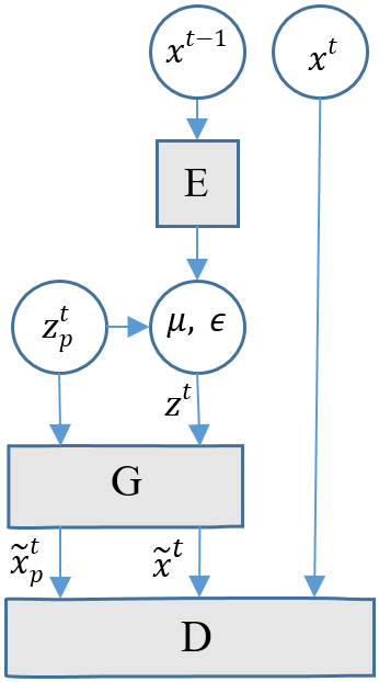
(a) Training framework.

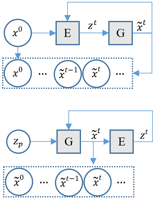
(b) Two testing frameworks.

Fig. 1: The training and testing frameworks of the proposed semi-recurrent hybrid VAE-GAN model ($E$: encoder, $G$: generator, and $D$: discriminator).

Considering the sequential data generation as a problem of generating a sequence of discrete frames, two problems need to be addressed: strong spatial correlation of the data in each of the frames, and the dependencies between them (temporal correlation). In this work, we propose a semi-recurrent convolution-based VAE-GAN for generating a sequence of individual frames where the above problems are efficiently addressed. In order to maintain strong local correlation of the data in each frame generated, we use CNN, which is a very effective architecture for this matter. Moreover, each frame is generated from the latent distribution of the previous frame encoded by an encoder. As a result, the dependencies across the frames are also kept.

Figure 1 illustrates the overall training and testing frameworks proposed in this work. The model includes an encoder, a generator (decoder), and a discriminator. To the best of our knowledge, this is the first hybrid VAE-GAN framework introduced for generating sequential data. The feasibility of this model is evaluated on piano music generation, which shows that the proposed framework is a viable way of training networks that model music, and has potential for modelling many other types of sequential data such as videos.

2 Preliminaries and Related Works

In recent years, deep generative models have achieved significant success, especially in generating natural images [13, 14, 15, 16, 17]. In these models, complex structures of the data can be learned using deep architectures with multiple layers. VAEs [13, 15] and GANs [14, 16, 17] are two powerful frameworks for learning deep generative models in an unsupervised manner.

2.1 Variational Auto-encoder (VAE)

A VAE consists of an encoder and a decoder [13]. The encoder, denoted by $q(z|x)$, encodes a data sample $x$ to a latent (hidden) representation $z$: $z\sim q(z|x)$. The decoder, denoted by $p(x|z)$, decodes the latent representation back to the probability distribution of the data (in data space): $\hat{x}\sim p(x|z)$.

The VAE regularizes the encoder by imposing a prior over the latent distribution $p(z)$ where $z\sim\mathcal{N}(0,I)$. The loss function of the VAE is the expected log likelihood with a regularizer:

$$\mathcal{L}_{VAE}=-\mathbb{E}_{q(z|x)}[\log p(x|z)]+KL(q(z|x)\|p(z))$$ (1)

where the first and second terms are the reconstruction loss and a prior regularization term that is the Kullback-Leibler (KL) divergence, respectively.

2.2 Generative Adversarial Network (GAN)

Another popular generative model is GAN in which two models are trained at the same time [14]. The generator model $G(z)$ captures the data distribution by mapping the latent $z$ to data space, while the discriminator model $D(x)\in[0,1]$ estimates the probability that $x$ is a real training sample or a fake sample synthesized by $G$. These two models compete in a two-player minimax game in which the objective function is to find a binary classifier $D$ that discriminates the real data from the fake (generated) ones, and simultaneously encourage $G$ to fit the true data distribution. This goal is achieved by minimizing/maximizing the binary cross entropy:

$$\mathcal{L}_{GAN}=\mathbb{E}_{x\sim p_{data}(x)}[\log D(x)]+\mathbb{E}_{z\sim p_{z}(z)}[\log(1-D(G(z)))]$$ (2)

where $G$ tries to minimize this objective against $D$ that tries to maximize it.

Although GANs are powerful generative models, they suffer from training instability and low-quality generated samples. Different approaches have been proposed to improve GANs. For example, Wasserstein GAN (WGAN) [18] used Wasserstein distance as an objective for training GANs to improve the stability of learning, Laplacian GAN (LAPGANs) [19] achieved coarse-to-fine conditional generation through Laplacian pyramids, and Deep Convolutional GAN (DCGAN) [16] proposed an effective and stable architecture for $D$ and $G$ using deeper CNNs to achieve remarkable image synthesis results.

2.3 Sequential Data Generation: Music Generation

Different learning-based approaches for sequential data generation, especially music, have been introduced by various researchers. In [20], a RNN-based architecture using LSTMs was proposed in which a piano-roll sequence of notes and chords were generated using an iterative feed-forward strategy. In [21] a Restricted Boltzmann Machine (RBM) was utilized for modeling and generating polyphonic music by learning a model from an audio corpus. DeepBach architecture [22], which was specialized for Bach’s chorales, combined two LSTMs and two feed-forward networks (forward and backward in time networks).

VAE, as one of the effective approaches considered for content generation, has been used by some researchers in order to generate musical content. In [2], a VAE-based method named Variational Recurrent Auto-Encoder (VRAE) was proposed in which the encoder and decoder parts were LSTMs. Variational Recurrent Autoencoder Supported by History (VRASH) [3] used the same architecture as in VRAE, but also used the output of the decoder back into the decoder. In [4], the objective function used in DeepBach was reformulated using VAE to have a better control on the embedding of the data into the latent space.

Although RNNs are more commonly used to model time-series signals, some non-RNN approaches have been introduced using CNNs [10, 23, 11]. A system for generating raw audio music waveforms named WaveNet was proposed in [10] in which an extended CNN called dilated causal convolution was incorporated. In this work, the authors argued that dilated convolutions allowed the receptive field to grow longer in a much cheaper way than using LSTMs. Another CNN-based architecture is convolutional RBM (C-RBM) [23], which was developed for the generation of MIDI polyphonic music. In this work, convolution was performed in the time domain to model temporally invariant motives.

Some works have exploited GANs for generating music [5, 11]. An example of the use of GAN is C-RNN-GAN [5] with both $G$ and $D$ being LSTMs in which the goal was to transform random noise into melodies. A bidirectional RNN was utilized in $D$ to take contexts from both past and future. In [11], a convolutional GAN architecture named MidiNet was proposed to generate pop music melodies from random noise (in piano-roll like format). In this approach, both $G$ and $D$ were composed of convolutional networks. Similar to what a recurrent network would do in considering the history, the information from previous musical measure was incorporated into intermediate layers.

3 Semi-Recurrent CNN-based VAE-GAN

In this section, the semi-recurrent hybrid VAE-GAN model proposed for generating temporal data such as music, is described. As illustrated in Figure 1, the model is composed of three units: the encoder ($E$), the generator/decoder ($G$), and the discriminator ($D$). In this work, the VAE decoder and the GAN generator are collapsed into one by letting them share parameters and training them jointly.

The main architecture of the three networks used in this work is CNNs. Convolutions are rarely used in modelling signals with invariance in time such as music, but they have been very successful in the models whose data has strong spatially local correlation such as images, which is also important for sequential data. In this work, we consider the input time-dependent data as a sequence of individual frames, which have internal spatial correlation. Thus, we exploit CNNs for separate generation of each of these frames, while keeping the dependencies across them as follows.

For each pair of sequential frames, the previous frame is encoded to its corresponding latent representation using $E$. Next, $G$ tries to generate (predict) the subsequent frame from the latent distribution of the previous frame. As a result, the history and the information from previous frames are incorporated for generating the next ones. The current real training frame in each pair and the synthesized frame are then forwarded to $D$ as real and fake data, respectively.

3.1 Formulation and Objective

Let $X=\{x^{0},...,x^{t-1},x^{t},...,x^{n}\}$ be a sequence from the training data with $n$ frames, the network $E$ maps a training frame $x^{t-1}$ (previous time frame) to the mean $\mu$ and the covariance $\epsilon$ of the latent vector:

$$\{\mu,\epsilon\}=E(x^{t-1})=q(z|x^{t-1}).$$ (3)

Then, the latent vector $z^{t}$ can be sampled as follows:

$$z^{t}=\mu+z^{t}_{p}\odot exp(\epsilon),$$ (4)

where $z^{t}_{p}\sim\mathcal{N}(0,I)$ and $\odot$ is the element-wise multiplication. In order to reduce the gap between the prior $p(z^{t})$ and the encoder’s distribution $q(z|x^{t-1})$ and measure how much information is lost, KL loss is used:

$$\mathcal{L}_{prior}=\mathcal{L}_{KL}=\frac{1}{2}(\mu^{T}\mu+sum(exp(\epsilon)-\epsilon-1)).$$ (5)

The network $G$ then generates two frames $\tilde{x}^{t}$ and $\tilde{x}^{t}_{p}$ by decoding the latent representations $z^{t}$ (sampled using $E$) and $z^{t}_{p}$ (sampled from a normal distribution) back to the data space, respectively:

$$\tilde{x}^{t}=G(z^{t}),\hskip 5.0pt\tilde{x}^{t}_{p}=G(z^{t}_{p}).$$ (6)

Element-wise reconstruction errors are generally inadequate for signals with invariances [8]. As a result, in order to measure the quality of the reconstructed samples in this work, the following pair-wise feature matching loss between the real data $x^{t}$ and the synthesized data $\tilde{x}^{t}$ and $\tilde{x}^{t}_{p}$ is utilized:

$$\mathcal{L}_{l}=\frac{1}{2}{\lVert D_{l}(x^{t})-D_{l}(\tilde{x}^{t})\rVert}^{2}_{2}+\frac{1}{2}{\lVert D_{l}(x^{t})-D_{l}(\tilde{x}^{t}_{p})\rVert}^{2}_{2},$$ (7)

where $D_{l}$ denotes the features (hidden representation) of an intermediate layer of the network $D$. Thus, the loss of network $E$ is calculated:

$$\mathcal{L}_{E}=\mathcal{L}_{l}+\mathcal{L}_{prior}.$$ (8)

In order to distinguish the real training data $x^{t}$ from the synthesized frames $\tilde{x}^{t}$ and $\tilde{x}^{t}_{p}$, the following objection function is minimized by $D$:

$$\mathcal{L}_{D}=-(\log D(x^{t})+\log(1-D(\tilde{x}^{t}))+\log(1-D(\tilde{x}^{t}_{p}))),$$ (9)

while $G$ tries to fool $D$ by minimizing

$$\mathcal{L}_{G}=-(\log D(\tilde{x}^{t})+\log D(\tilde{x}^{t}_{p}))+\mathcal{L}_{l},$$ (10)

where $\mathcal{L}_{l}$ is the pair-wise feature matching loss (Equation 7), which is a shared error signal between $E$ and $G$.

Finally, our goal is to minimize the following hybrid loss function: $\mathcal{L}=\mathcal{L}_{E}+\mathcal{L}_{D}+\mathcal{L}_{G}$.

4 Experiments: Piano Music Generation

We applied the proposed approach to piano music generation. The source code and some generated samples are shared on GitHub. In this experiment, we used the Nottingham dataset as our training data, which contains 695 pieces of folk piano music in MIDI file format. Each MIDI file was divided into separate bars, and a bar is represented by a real-valued 2-D matrix $x\in[0,1]^{h\times w}$ where $h$ and $w$ represent the number of MIDI notes/pitches (i.e., $h=88$ in this work) and the number of time steps (i.e., $w=16$ with pitch sampling of 0.125sec), respectively. The value of each element of the matrix is the velocity (volume) of a note at a certain time step. The sequence of $n$ bars is denoted by $X=\{x^{0},...,x^{t-1},x^{t},...,x^{n}\}$ where $x^{t-1}$ and $x^{t}$ are two sequential bars.

The details of the networks $E$, $G$, and $D$ are summarized in Table 1. The output layer of $E$ is a fully-connected layer with 256 hidden units where its first and second 128 units are respectively considered as the mean $\mu$ and covariance $\epsilon$ used for representing the latent $z^{t}$ of dimension 128 (Equations 3 and 4). The latent $z^{t}$ and a normal distribution $z^{t}_{p}$ (of dimension 128) are projected to $G$ to output the synthesized bars $\tilde{x}^{t},\tilde{x}^{t}_{p}\in[0,1]^{88\times 16}$. Before the Tanh layer of $G$, another convolution is applied to map to the number of output channels (that is 1 in this work). An extra convolution is also applied before the Sigmoid layer of $D$ to represent the output by a 1-D feature map, which is used as $D_{l}$ for calculating the pair-wise feature matching loss (Equation 7). This network takes the 2-D matrices $x^{t}$ and $\tilde{x}^{t}$ as inputs and predicts whether they are real or generated MIDI bars.

Table 1: The network architecture of the encoder (E), generator (G), and discriminator (D). AF, In, and Out are respectively the activation functions used after each conv/deconv layer, the input, and the output of each network.

	Layers (filters)	Size	AF	In	Out
E	conv (8, 16, 32), Fully-connected layer	5$\times$5 stride=2	ELU	$x^{t-1}$	{$\mu,\epsilon$}
G	deconv (64, 32, 16, 8), Tanh layer	3$\times$3 stride=1	ReLU	$z^{t},z^{t}_{p}$	$\tilde{x}^{t},\tilde{x}^{t}_{p}$
D	conv (8, 16, 32, 64), Sigmoid layer	3$\times$3 stride=1	LeakyReLU	$x^{t},\tilde{x}^{t}$	0 or 1

All models were trained with mini-batch stochastic gradient descent (SGD) with a mini-batch size of 64. The Adam optimizer with momentum of 0.5 and learning rate of 0.0005 for $E$ and $G$, and 0.0001 for $D$ was used. In order to keep the losses corresponding to $E$, $G$, and $D$ balanced in each iteration, we trained $E$ and $G$ twice and $D$ once.

Two models illustrated in Figure 1 were proposed to sequentially generate music with an arbitrary number of bars. In model 1 (top model in Figure 1), the input to $E$, denoted by $x^{0}$, is a bar randomly selected from training data samples, which is considered as the first bar of the generated music. $x^{0}$ is then mapped to the latent $z^{1}$ using $E$. $G$ synthesizes the next bar $\tilde{x}^{1}$ by decoding $z^{1}$ back to the data space. By feeding the generated bar $\tilde{x}^{1}$ to $E$, this process is repeatedly performed to generate a sequence of bars. In model 2 (bottom model in Figure 1), the same recurrent process is applied, but the first bar is also a bar synthesized using $G$ from a random noise $z_{p}$. Two 5-bar sample music generated using model 1 (top model in Figure 1) are illustrated in Figure 2.

Fig. 2: Two 5-bar sample music generated using the proposed testing model 1 (top model in Figure 1).

4.1 Results

In order to evaluate the music samples generated using our approach, the following measurements were taken into account [5]: scale consistency (the percentage for the best matching musical scale that a sample is part of), uniqueness (the percentage of unique tones used in a sample), velocity span (the velocity range in which the tones are played), recurrence (repetitions of short subsequences of length 2 in a sample), tone span (the number of half-tone steps between the lowest and the highest tones in a sample), and diversity (the average pairwise Levenshtein edit distance [24] of the generated data ). Figure 3 shows the results of evaluating $\approx 2,500$ generated pieces of music of length 10 seconds (i.e., 5 two-second bars).

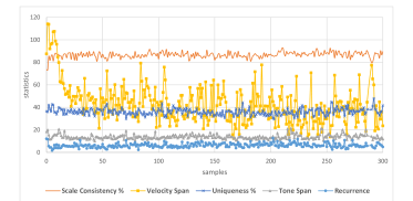
Fig. 3: Measurements used for evaluating $\approx{2,500}$ music samples generated at 300 epochs: scale consistency, intensity span, uniqueness, tone span, and recurrence.

As seen in Figure 3, the scale consistency (with an average of $\approx 87\%$) shows that the generated music significantly follows the standard scales in all samples, which outperforms C-RNN-GAN [5] with an average of $\approx 75\%$. A variety of velocities exist in the music generated, which is illustrated by the oscillating velocity span. The average percentage of the unique tones used in the generated piece is $\approx 37\%$. Compared to the velocity span, less variability is seen in the tone span (with minimum and maximum of 10 and 21) of the generated music due to the low tone span in the training samples (the majority of the music in the dataset is played in 1 or 2 octaves). The number of 2-tone repetitions is $\approx 7$ in average. Diversity is another metric we took into account to evaluate how realistic the generated music sounds. Compared to ORGAN [6] with an average of 0.551, a higher diversity with an average of $\approx 0.59$ was achieved in this work.

5 Conclusion

A semi-recurrent VAE-GAN model for generating sequential data was presented in this work. The model consisted of three networks (encoder, generator, and discriminator) in which convolutions were utilized to spatially learn the local correlation of the data in individual frames. Each frame was sampled from a latent distribution obtained by mapping the previous frame using the encoder. As a consequence, the consistencies between the frames in a generated sequence was also preserved. Our experiments on piano music generation presented promising results, which were comparable to the state-of-the-art. One potential direction of this work is to use this framework for modelling and generating other types of sequential data such as video.

6 Acknowledgement

This work was supported by the Natural Sciences and Engineering Research Council (NSERC) of Canada under grant RGPIN312262 and RGPAS478109.

References

- [1] R. Pascanu, T. Mikolov, and Y. Bengio, “On the difficulty of training recurrent neural networks,” in ICML, 2013, pp. 1310–1318.
- [2] O. Fabius and J. R. van Amersfoort, “Variational recurrent auto-encoders,” arXiv preprint arXiv:1412.6581, 2014.
- [3] A. Tikhonov and I. P Yamshchikov, “Music generation with variational recurrent autoencoder supported by history,” arXiv preprint arXiv:1705.05458, 2017.
- [4] G. Hadjeres, F. Nielsen, and F. Pachet, “GLSR-VAE: Geodesic latent space regularization for variational autoencoder architectures,” arXiv preprint arXiv:1707.04588, 2017.
- [5] O. Mogren, “C-RNN-GAN: Continuous recurrent neural networks with adversarial training,” arXiv preprint arXiv:1611.09904, 2016.
- [6] G. L. Guimaraes, B. Sanchez-Lengeling, P. L. Farias, and A. Aspuru-Guzik, “Objective-reinforced generative adversarial networks (ORGAN) for sequence generation models,” arXiv preprint arXiv:1705.10843, 2017.
- [7] L. Yu, W. Zhang, J. Wang, and Y. Yu, “SeqGAN: Sequence generative adversarial nets with policy gradient.,” in AAAI, 2017, pp. 2852–2858.
- [8] A. B. Larsen, S. Sønderby, H. Larochelle, and O. Winther, “Autoencoding beyond pixels using a learned similarity metric,” arXiv preprint arXiv:1512.09300, 2015.
- [9] A. Makhzani, J. Shlens, N. Jaitly, I. Goodfellow, and B. Frey, “Adversarial autoencoders,” arXiv preprint arXiv:1511.05644, 2015.
- [10] A. Oord, S. Dieleman, H. Zen, K. Simonyan, O. Vinyals, A. Graves, N. Kalchbrenner, A. Senior, and K. Kavukcuoglu, “Wavenet: A generative model for raw audio,” arXiv preprint arXiv:1609.03499, 2016.
- [11] L. Yang, S. Chou, and Y. Yang, “Midinet: A convolutional generative adversarial network for symbolic-domain music generation using 1D and 2D conditions,” arXiv preprint arXiv:1703.10847, 2017.
- [12] J. Briot, G. Hadjeres, and F. Pachet, “Deep learning techniques for music generation-a survey,” arXiv preprint arXiv:1709.01620, 2017.
- [13] D. P. Kingma and M. Welling, “Auto-encoding variational bayes,” arXiv preprint arXiv:1312.6114, 2013.
- [14] I. Goodfellow, J. Pouget-Abadie, M. Mirza, B. Xu, D. Warde-Farley, S. Ozair, A. Courville, and Y. Bengio, “Generative adversarial nets,” in NIPS, 2014, pp. 2672–2680.
- [15] D. Jimenez Rezende, S. Mohamed, and D. Wierstra, “Stochastic backpropagation and approximate inference in deep generative models,” arXiv preprint arXiv:1401.4082, 2014.
- [16] A. Radford, L. Metz, and S. Chintala, “Unsupervised representation learning with deep convolutional generative adversarial networks,” arXiv preprint arXiv:1511.06434, 2015.
- [17] T. Salimans, I. Goodfellow, W. Zaremba, V. Cheung, A. Radford, and X. Chen, “Improved techniques for training GANs,” in NIPS, 2016, pp. 2234–2242.
- [18] M. Arjovsky, S. Chintala, and L. Bottou, “Wasserstein GAN,” arXiv preprint arXiv:1701.07875, 2017.
- [19] E. L. Denton, S. Chintala, R. Fergus, et al., “Deep generative image models using a laplacian pyramid of adversarial networks,” in NIPS, 2015, pp. 1486–1494.
- [20] D. Eck and J. Schmidhuber, “A first look at music composition using LSTM recurrent neural networks,” IDSIA, vol. 103, 2002.
- [21] N. Boulanger-Lewandowski, Y. Bengio, and P. Vincent, “Modeling temporal dependencies in high-dimensional sequences: Application to polyphonic music generation and transcription,” arXiv preprint arXiv:1206.6392, 2012.
- [22] G. Hadjeres and F. Pachet, “DeepBach: a steerable model for bach chorales generation,” arXiv preprint arXiv:1612.01010, 2016.
- [23] S. Lattner, M. Grachten, and G. Widmer, “Imposing higher-level structure in polyphonic music generation using convolutional restricted boltzmann machines and constraints,” arXiv preprint arXiv:1612.04742, 2016.
- [24] A. Habrard, J. M. Iñesta, D. Rizo, and M. Sebban, “Melody recognition with learned edit distances,” in SSPR/SPR, 2008, pp. 86–96.