“Big Three Dragons”: a $z=7.15$ Lyman Break Galaxy Detected in [Oiii] $88$ , [Cii] $158$ , and Dust Continuum with ALMA

Abstract

We present new ALMA observations and physical properties of a Lyman Break Galaxy at $z=7.15$. Our target, B14-65666, has a bright ultra-violet (UV) absolute magnitude, $M_{\rm UV}\approx-22.4$, and has been spectroscopically identified in Ly$\alpha$ with a small rest-frame equivalent width of $\approx 4$ Å. Previous HST image has shown that the target is comprised of two spatially separated clumps in the rest-frame UV. With ALMA, we have newly detected spatially resolved [Oiii] 88 , [Cii] 158 , and their underlying dust continuum emission. In the whole system of B14-65666, the [Oiii] and [Cii] lines have consistent redshifts of $7.1520\pm 0.0003$, and the [Oiii] luminosity, $(34.4\pm 4.1)\ \times 10^{8}$ $L_{\rm\odot}$, is about three times higher than the [Cii] luminosity, $(11.0\pm 1.4)\ \times 10^{8}$ $L_{\rm\odot}$. With our two continuum flux densities, the dust temperature is constrained to be $T_{\rm d}$ $\approx 50-60$ K under the assumption of the dust emissivity index of $\beta_{\rm d}=2.0-1.5$, leading to a large total infrared luminosity of $L_{\rm TIR}$ $\approx 1\times 10^{12}$ $L_{\rm\odot}$. Owing to our high spatial resolution data, we show that the [Oiii] and [Cii] emission can be spatially decomposed into two clumps associated with the two rest-frame UV clumps whose spectra are kinematically separated by $\approx 200$ km s^-1. We also find these two clumps have comparable UV, infrared, [Oiii], and [Cii] luminosities. Based on these results, we argue that B14-65666 is a starburst galaxy induced by a major-merger. The merger interpretation is also supported by the large specific star-formation rate (defined as the star-formation rate per unit stellar mass), sSFR $=260^{+119}_{-57}$ Gyr^-1, inferred from our SED fitting. Probably, a strong UV radiation field caused by intense star formation contributes to its high dust temperature and the [Oiii]-to-[Cii] luminosity ratio.

1 Introduction

Understanding properties of galaxies during reionization, at redshift $z\gtrsim 6-7$, is important. While a large number of galaxy candidates are selected with a dropout technique at $z\gtrsim 7$ (e.g., Ellis et al. 2013; Bouwens et al. 2014; Oesch et al. 2018), the spectroscopic identifications at $z\gtrsim 7$ remain difficult (e.g., Stark et al. 2017 and references therein). This is mainly due to the fact that the most prominent hydrogen Ly$\alpha$ line is significantly attenuated by the intergalactic medium (IGM).

With the advent of the Atacama Large Millimeter/Submillimeter Array (ALMA) telescope, it has become possible to detect rest-frame far-infrared (FIR) fine structure lines in star-forming galaxies at $z>5$ (e.g., Capak et al. 2015; Maiolino et al. 2015). A most commonly used line is [Cii] 158 , which is one of the brightest lines in local galaxies (e.g., Malhotra et al. 1997; Brauher et al. 2008). To date, more than 21 [Cii] detections are reported at $5\lesssim z\lesssim 7$ (Carniani et al. 2018b and references therein; Pentericci et al. 2016; Matthee et al. 2017; Smit et al. 2018).

However, based on a compiled sample with [Cii] observations at $z\gtrsim 5$, Harikane et al. (2018) and Carniani et al. (2018b) have revealed that [Cii] may be weak for galaxies with strong Ly$\alpha$ emission, so-called Ly$\alpha$ emitters (LAEs; rest-frame Ly$\alpha$ equivalent widths EW₀(Ly$\alpha$) $\gtrsim 20-30$ Å). Harikane et al. (2018) have interpreted the trend with photoionization models of CLOUDY (Ferland et al. 2013) implemented in spectral energy distribution (SED) models of BEAGLE (Chevallard & Charlot 2016). The authors show that low metallicity or high ionization states in LAEs lead to weak [Cii]. Theoretical studies also show that such ISM conditions lead to the decrease in the [Cii] luminosity (Vallini et al. 2015, 2017; Olsen et al. 2017; Lagache et al. 2018). If we assume that $z\gtrsim 7$ galaxies in general have low metallicity or high ionization states, [Cii] may not be the best line to spectroscopically confirm $z\gtrsim 7$ galaxies. Indeed, a number of null-detections of [Cii] are reported at $z\gtrsim 7$ (e.g., Ota et al. 2014; Schaerer et al. 2015; Maiolino et al. 2015; Inoue et al. 2016).

In fact, based on Herschel spectroscopy for local dwarf galaxies, Cormier et al. (2015) have demonstrated that [Oiii] 88  becomes brighter than [Cii]  at low metallicity (see also Malhotra et al. 2001). Based on calculations of CLOUDY, Inoue et al. (2014b) also theoretically predict that the [Oiii] line at high-$z$ should be bright enough to be detected with ALMA.

Motivated by these backgrounds, we are conducting follow-up observations of the [Oiii] 88  line for $z>6$ galaxies with ALMA. After the first detection of [Oiii] in the reionization epoch in Inoue et al. (2016) at $z=7.21$, the number of [Oiii] detections is rapidly increasing. There are currently ten objects with [Oiii] detections at $z\approx 6-9$ (Carniani et al. 2017; Laporte et al. 2017; Marrone et al. 2018; Hashimoto et al. 2018a; Tamura et al. 2018, Hashimoto et al. 2018b; Walter et al. 2018). Remarkably, Hashimoto et al. (2018a) have detected [Oiii] in a $z=9.11$ galaxy with a high significance level of $7.4\sigma$. Importantly, [Oiii] is detected from all the targeted galaxies (six detections out of six objects) from our team, i.e., the success rate is currently 100% . These results clearly demonstrate that [Oiii] is a powerful tool to confirm $z>6$ galaxies.

Inoue et al. (2016) have also investigated the FIR line ratio at $z>7$. In a combination with the null detection of [Cii], the authors have shown that their $z=7.21$ LAE has a line ratio of [Oiii]/[Cii] $>12$ ($3\sigma$). The line ratio would give us invaluable information on properties of the interstellar medium (ISM). Given the fact that [Oiii] originates only from HII regions whereas [Cii] originates both from HII regions and photo-dissociated regions (PDRs), Inoue et al. (2016) have interpreted the high line ratio as the $z=7.21$ LAE having highly ionized HII regions but less PDRs. Such properties would lead to a high escape fraction of ionizing photons, which is a key parameter to understand reionization. Therefore, it is of interest to understand if a high line ratio is common in high-$z$ galaxies (Inoue et al. 2016).

In this study, we present new ALMA observations and physical properties of an Lyman Break Galaxy (LBG) at $z=7.15$. Our target, B14-65666, is a very ultra-violet (UV) bright LBG with an absolute magnitude, $M_{\rm UV}\approx-22.4$ (Bowler et al. 2014, 2017, 2018). With the Faint Object Camera and Spectrograph (FOCAS) on the Subaru telescope, Furusawa et al. (2016) have spectroscopically detected Ly$\alpha$ at the significance level of $5.5\sigma$. The authors find that B14-65666 has a small EW₀(Ly$\alpha$) of $3.7^{+1.7}_{-1.1}$ Å. In addition, based on observations with the Hubble Space Telescope (HST) Wide Field Camera 3 (WFC3) F140W band image, Bowler et al. (2017) have revealed that B14-65666  is comprised of two components in the rest-frame UV with a projected separation of $\approx 2-4$ kpc. At high-$z$, such a complicated structure is often interpreted in terms of a merger or clumpy star formation. The authors have argued that the large star-formation rate (SFR) inferred from the UV luminosity could be naturally explained if the system is a merger-induced starburst. More recently, with ALMA Band 6 observations, Bowler et al. (2018) have detected dust continuum emission at the peak significance level of $5.2\sigma$, which is the third detection of dust emission in normal star-forming galaxies at $z>7$ (cf., Watson et al. 2015; Laporte et al. 2017 see also Knudsen et al. 2017).

In ALMA Cycle 4, we have performed high spatial resolution follow-up observations of B14-65666 with beam size of $\approx 0^{\prime\prime}.3\times 0^{\prime\prime}.2$ ($0^{\prime\prime}.3\times 0^{\prime\prime}.3$) in Band 6 (Band 8). In ALMA Cycle 5, we have also obtained deeper Band 8 data with a slightly larger beam size of $\approx 0^{\prime\prime}.4\times 0^{\prime\prime}.4$. We successfully detect spatially resolved [Cii], [Oiii], and dust continuum emission in two bands, making B14-65666 the first object at $z\gtrsim 6$ with a complete set of these three features. The spatially resolved data enable us to investigate the velocity gradients of the [Cii] and [Oiii] lines. These emission lines also allow us to investigate the Ly$\alpha$ velocity offset with respect to the systemic, $\Delta v_{\rm Ly\alpha}$, which is an important parameter to understand reionization (e.g., Choudhury et al. 2015; Mason et al. 2018a, b). The dust continuum emission also offers us invaluable information on the ISM properties of B14-65666. We also derive physical quantities such as the stellar age, the stellar mass ($M_{\rm*}$), and the SFR. With these quantities, we will discuss kinematical, morphological, and ISM properties of B14-65666.

This paper is organized as follows. In §2, we describe our data. In §3, we measure [Cii] and [Oiii] quantities. Dust properties are presented in §4, followed by results on luminosity ratios in §5. In §6, we perform spectral energy distribution (SED) fitting. In §7, we derive $\Delta v_{\rm Ly\alpha}$ in B14-65666, and statistically examine $\Delta v_{\rm Ly\alpha}$ at $z\approx 6-8$. Discussions in the context of (i) properties of B14-65666 and (ii) reionization are presented in §8, followed by our conclusions in §9. Throughout this paper, magnitudes are given in the AB system (Oke & Gunn, 1983), and we assume a $\Lambda$CDM cosmology with $\Omega_{\small m}=0.272$, $\Omega_{\small b}=0.045$, $\Omega_{\small\Lambda}=0.728$ and $H_{\small 0}=70.4$ km s^-1 Mpc^-1 (Komatsu et al. 2011). The solar luminosity, $L_{\rm\odot}$, is $3.839\times 10^{33}$ erg s^-1.

Summary of ALMA Observations. Date Baseline lengths $N_{\rm ant}$ Central frequencies of SPWs Integration time PWV (YYYY-MM-DD) (m) (GHz) (min.) (mm) (1) (2) (3) (4) (5) (6) Band 6 (Cycle 4) 2017-07-09 $16-2647$ 40 218.78, 216.98, 232.66, 234.48 37.80 0.45 2017-07-09 $16-2647$ 40 218.78, 216.98, 232.66, 234.48 37.80 0.44 2017-07-09 $16-2647$ 40 218.78, 216.98, 232.66, 234.48 37.80 0.42 Band 8 (Cycles 4 + 5) 2016-11-14 $15-918$ 40 405.43, 403.61, 415.47, 417.23 14.45 0.58 2016-11-15 $15-918$ 40 405.43, 403.61, 415.47, 417.23 39.72 0.63 2018-04-06 $15-483$ 43 404.09, 405.98, 416.02, 417.60 47.60 0.86 2018-05-01 $15-500$ 43 404.09, 405.98, 416.02, 417.60 45.20 0.95 2018-05-01 $15-500$ 43 404.09, 405.98, 416.02, 417.60 45.22 0.83 2018-05-04 $15-500$ 43 404.09, 405.98, 416.02, 417.60 45.22 0.69 2018-05-05 $15-500$ 43 404.09, 405.98, 416.02, 417.60 45.17 0.81 Note. (1) The observation date; (2) the ALMA’s baseline length; (3) the number of antenna used in the observation; (4) the central frequencies of the four spectral windows (SPWs); (5) the on-source integration time; (6) the precipitable water vapor.

2 Observations and Data

2.1 ALMA Band 6 Observations

As summarized in Table 1, we observed B14-65666 with ALMA in Band 6 targeting [Cii] 158  in Cycle 4 (ID 2016.1.00954.S, PI: A. K. Inoue). The antenna configuration was C40-6, and the on-source exposure times was 114 minutes. We used four spectral windows (SPWs) with 1.875 GHz bandwidths in the Frequency Division Mode (FDM), totaling the band width of 7.5 GHz. Two SPWs with a 7.813 MHz resolution was used to target the line. One of the two SPWs was centered on the Ly$\alpha$ frequency and the other was centered at a higher frequency (i.e, a shorter wavelength) with a small overlap in frequency, taking into account the possible redward velocity offset of the Ly$\alpha$ line with respect to the systemic redshift (e.g., Steidel et al. 2010; Hashimoto et al. 2013). The remaining two SPWs with a 31.25 MHz resolution were used to observe dust continuum emission at $\approx 163$ . A quasar, J0948+0022 (J1058+0133) was used for phase (bandpass) calibrations, and two quasars, J1058+0133 and J0854+2006, were used for flux calibrations (Appendix 2 Table B). The flux calibration uncertainty was estimated to be $\lesssim$ 10%. The data were reduced and calibrated using the Common Astronomy Software Application (CASA; McMullin et al. 2007) pipeline version 4.7.2. Using the CLEAN task, we produced two images and cubes with different weighting: (1) The natural weighting to maximize point-source sensitivity on which we perform photometry and (2) the Briggs weighting with the robust parameter of 0.3 to investigate morphological properties. To create a pure dust continuum image, we collapsed all off-line channels. To create a pure line image, we subtracted continuum using the off-line channels in the line cube with the CASA task uvcontsub. In Table 2.2, we summarize the r.m.s. levels, the spatial resolutions, and the beam position angles for the continuum images with two weighting.

2.2 ALMA Band 8 Observations

In Cycles 4 and 5, we also observed B14-65666 with ALMA in Band 8 targeting [Oiii] 88  (IDs 2016.1.00954.S and 2017.1.00190.S; PIs: A. K. Inoue; Table 1). The antenna configuration was C40-4 (C43-3) for the Cycle 4 (5) observations, and the total on-source exposure times was 282 minutes. The observation strategy was the same as that used in Band 6. The combinations of two quasars, (J0948+0022 and J1028-0236), (J1058+0133 and J1229+0203), and (J1058+0133 and J1229+0203) were used for phase, bandpass, and flux calibrations, respectively (Appendix 2 Table B). The flux calibration uncertainty was estimated to be $\lesssim$ 10%. The Cycles 4 and 5 datasets were first reduced and calibrated with the CASA pipeline versions 4.7.0 and 5.1.1, respectively, and then combined into a single measurement set with the CASA task concat. We created images and cubes with the natural weighting using the CLEAN task. In Table 2.2, we summarize the r.m.s. level, the beam size, and the beam position angle for the continuum image.

Summary of ALMA data. Data $\sigma_{\rm cont}$ Beam FWHMs PA ($\mu$Jy beam^-1) (arcsec $\times$ arcsec) (deg.) (1) (2) (3) (4) Band 6 (natural) 9.5 $0.29\times 0.23$ $-60$ Band 6 (Briggs) 11.0 $0.23\times 0.12$ $-70$ Band 8 (natural) 29.4 $0.39\times 0.37$ $+62$ Note. (1) The ALMA Band used. Weighting is specified in the parenthesis; (2) the $1\sigma$ r.m.s. level of the continuum image; (3) the ALMA’s beam FWHM in units of arcsec $\times$ arcsec; (5) the ALMA’s beam position angle in units of degree.

3 [Cii] 158  and [Oiii] 88  lines

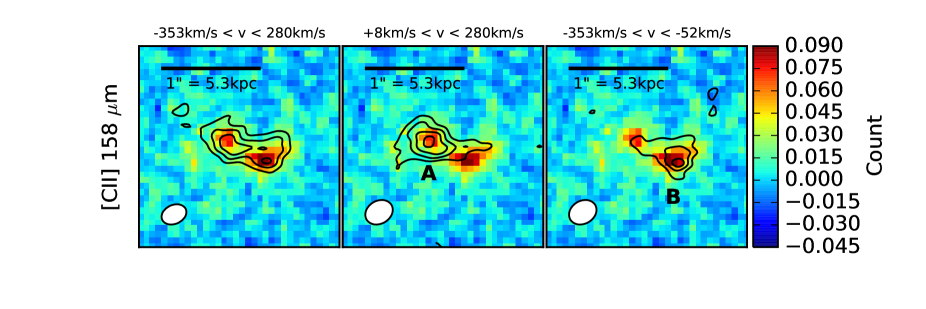
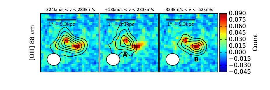
Figure 1: Top and bottom panels show [Cii] and [Oiii] contours overlaid on the $2^{\prime\prime}.0\times 2^{\prime\prime}.0$ cutout image of HST F140W, respectively. The left, middle, and right panels correspond to the line image for the whole system, clump A, and clump B, respectively. The velocity range used to extract the images are indicated above the panels, where the velocity zero point is defined as the systemic redshift, $z_{\rm sys}$ $=$ 7.1520. (Top) [Cii] line contours drawn at ($3$, $5$, $7$, $9$)$\times\sigma$, where $\sigma\approx$ 19, 12, and 13 mJy beam^-1 km s^-1 for the left, middle and right panel, respectively. (Bottom) [Oiii] line contours drawn at ($3$, $5$, $7$, $9$, $11$)$\times\sigma$, where $\sigma\approx$ 48, 31, and 31 mJy beam^-1 km s^-1 for the left, middle and right panel, respectively. In each panel, contours are shown by the solid lines and the ellipse at lower left indicates the synthesized beam size of ALMA.

3.1 Measurements for the Whole System

In Band 6 (8) data, to search for an emission line, we have created a data cube by binning three (six) native channels, resulting in a velocity resolution of $\approx 30\ (33)$ km s^-1. At the B14-65666 position determined in the HST image, we find a supposed [Cii] ([Oiii]) feature at around 233.12 (416.27) GHz. This frequency region is free from atmospheric absorption features. In Band 6 (8), we have then created a velocity-integrated intensity image between 232.9 and 233.4 GHz (415.8 and 416.7 GHz) corresponding to $\approx$ 600 (600) km s^-1.

The top left and bottom left panels of Figure 1 show [Cii] and [Oiii] contours overlaid on the HST F140W images, respectively, whose detailed astrometry analyses are presented in Appendix 1, and our measurements are summarized in Table 3.1. With our spatial resolution, [Cii] and [Oiii] are spatially resolved. Assuming a 2D Gaussian profile for the velocity-integrated intensity, we measure the beam-deconvolved size of [Cii] to be $(0^{\prime\prime}.84\pm 0^{\prime\prime}.12)\times(0^{\prime\prime}.27\pm 0^{\prime\prime}.05)$, where the first and second values represent the FWHMs of the major and minor-axis, respectively, with a positional angle (PA) of $74^{\circ}\pm 4^{\circ}$. At $z=7.15$, the physical size corresponds to $(4.5\pm 0.6)\times(1.4\pm 0.3)$ kpc². Likewise, we obtain the beam-deconvolved size of [Oiii] to be $(0^{\prime\prime}.71\pm 0^{\prime\prime}.10)\times(0^{\prime\prime}.41\pm 0^{\prime\prime}.11)$, corresponding to $(3.8\pm 0.5)\times(2.2\pm 0.6)$ kpc² at $z=7.15$, with PA = $76^{\circ}\pm 12^{\circ}$. The size and PA values of [Cii] and [Oiii] are consistent with each other.

Summary of observational results of B14-65666. Parameters Total Clump A Clump B R.A. 10:01:40.69 10:01:40.70 10:01:40.67 Dec. +01:54:52.42 +01:54:52.64 +01:54:52.47 $M_{\rm 1500}$ [AB mag.] -22.4 -21.5 -21.8 $L_{\rm UV}$ [$10^{11}$ $L_{\rm\odot}$] 2.0 0.9 1.1 $z_{\rm[OIII]}$ $7.1521\pm 0.0004$ $7.1523\pm 0.0004$ $7.1488\pm 0.0004$ $z_{\rm[CII]}$ $7.1521\pm 0.0004$ $7.1536\pm 0.0004$ $7.1478\pm 0.0005$ $z_{\rm sys.}$ ^a $7.1521\pm 0.0003$ $7.1530\pm 0.0003$ $7.1482\pm 0.0003$ $z_{\rm Ly\alpha}$^b $7.1730\pm 0.0012$ - - $\Delta v_{\rm Ly\alpha}$ [km s^-1] $772\pm 45\pm 100$ - - [Oiii] integrated flux [Jy km s^-1] $1.50\pm 0.18$ $0.92\pm 0.14$ $0.57\pm 0.09$ [Cii] integrated flux [Jy km s^-1] $0.87\pm 0.11$ $0.47\pm 0.07$ $0.38\pm 0.06$ FWHM([Oiii]) [km s^-1] $429\pm 37$ $325\pm 32$ $267\pm 34$ FWHM([Cii]) [km s^-1] $349\pm 31$ $347\pm 29$ $284\pm 40$ [Oiii] deconvolved size^c [kpc²] $(3.8\pm 0.5)\times(2.2\pm 0.6)$ $(3.8\pm 0.7)\times(3.0\pm 0.6)$ $(3.1\pm 0.6)\times(1.1\pm 0.7)$ [Cii] deconvolved size^c [kpc²] $(4.5\pm 0.6)\times(1.4\pm 0.3)$ $(3.3\pm 0.5)\times(1.5\pm 0.3)$ $(2.5\pm 0.6)\times(1.4\pm 0.5)$ $M_{\rm dyn}$^d [$10^{10}$ $M_{\rm\odot}$] $8.8\pm 1.9$ $5.7\pm 1.6$ $3.1\pm 1.1$ [Oiii] luminosity [$10^{8}$ $L_{\rm\odot}$] $34.4\pm 4.1$ $21.1\pm 3.2$ $13.0\pm 2.1$ [Cii] luminosity [$10^{8}$ $L_{\rm\odot}$] $11.0\pm 1.4$ $6.0\pm 0.9$ $4.9\pm 0.8$ Ly$\alpha$ luminosity [$10^{8}$ $L_{\rm\odot}$] $6.8\pm 1.3$ - - [Oiii]-to-[Cii] luminosity ratio $3.1\pm 0.6$ $3.5\pm 0.8$ $2.7\pm 0.6$ $S_{\rm\nu,90}$ [$\mu$Jy] $470\pm 128$ $208\pm 83$ $246\pm 73$ $S_{\rm\nu,163}$ [$\mu$Jy] $130\pm 25$ $41\pm 23$ $87\pm 26$ dust deconvolved size [kpc²] $(3.8\pm 1.1)\times(0.8\pm 0.5)$ $<1.6\times 1.2$^e $<1.6\times 1.2$^e $L_{\rm TIR}$ ($T_{\rm d}$$=48$K, $\beta_{\rm d}$$=$2.0) [$10^{11}$ $L_{\rm\odot}$] $9.1\pm 1.8$ $2.9\pm 1.6$ $6.1\pm 1.8$ $L_{\rm TIR}$ ($T_{\rm d}$$=54$K, $\beta_{\rm d}$$=$1.75) [$10^{11}$ $L_{\rm\odot}$] $10.5\pm 2.0$ $3.3\pm 1.9$ $7.0\pm 2.1$ $L_{\rm TIR}$ ($T_{\rm d}$$=61$K, $\beta_{\rm d}$$=$1.5) [$10^{11}$ $L_{\rm\odot}$] $12.0\pm 2.3$ $3.8\pm 2.1$ $8.0\pm 2.4$ $M_{\rm d}$ ($T_{\rm d}$$=48$K, $\beta_{\rm d}$$=$2.0) [$10^{6}$ $M_{\rm\odot}$] $11.1\pm 2.1$ $3.5\pm 2.0$ $7.4\pm 2.2$ $M_{\rm d}$ ($T_{\rm d}$$=54$K, $\beta_{\rm d}$$=$1.75) [$10^{6}$ $M_{\rm\odot}$] $9.4\pm 1.8$ $3.0\pm 1.7$ $6.3\pm 1.9$ $M_{\rm d}$ ($T_{\rm d}$$=61$K, $\beta_{\rm d}$$=$1.5) [$10^{6}$ $M_{\rm\odot}$] $8.1\pm 1.6$ $2.6\pm 1.4$ $5.4\pm 1.6$ Note. ^a The systemic redshift, $z_{\rm sys.}$, is calculated as the $S/N$-weighted mean redshift of $z_{\rm[OIII]}$ and $z_{\rm[CII]}$.
^b The value is different from the original value in Furusawa et al. (2016), $z_{\rm Ly\alpha}$$=7.168$, to take into account air refraction and the motion of the observatory (see §7).
^c The values represent major and semi-axis FWHM values of a 2D Gaussian profile.
^d The dynamical mass of individual clumps is estimated based on the virial theorem assuming the random motion (see §3.3). The total dynamical mass of the system is assumed to be the summation of the dynamical masses of the clumps.
^eWe present the beam size of Band 6, i.e., higher angular resolution image, as the upper limit because the emission is unresolved in the individual clumps.
The total infrared luminosity, $L_{\rm TIR}$, is estimated by integrating the modified-black body radiation at $8-1000$ . For the dust temperature and the emissivity index values, we assume the three combinations of ($T_{\rm d}$ [K], $\beta_{\rm d}$) = (48, 2.0), (54, 1.75), and (61, 1.5) (see §4 for the choices of these values. The dust mass, $M_{\rm d}$, is estimated with a dust mass absorption coefficient $\kappa=\kappa_{\rm 0}(\mu/\nu_{\rm 0})^{\beta_{\rm d}}$, where we assume $\kappa_{\rm 0}=10$ cm² g^-1 at 250  (Hildebrand 1983).

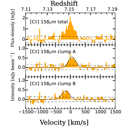
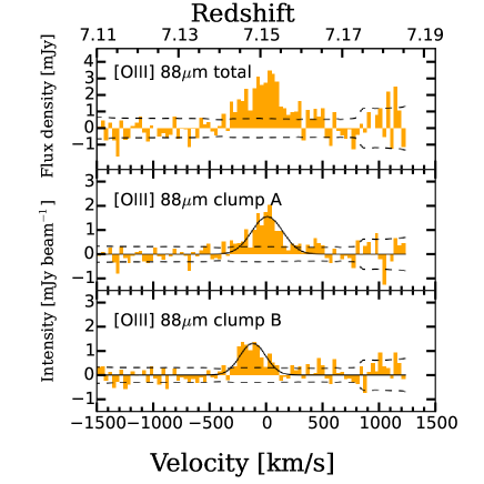
Figure 2: (Left) Top panel shows the [Cii] spectrum in units of mJy extracted from the region with $>3\sigma$ detections in the velocity-integrated intensity image shown in Figure 1. Middle and bottom panels show the [Cii] spectra in units of mJy beam^-1 extracted at the positions of clumps A and B, respectively. The black line denotes the best-fit Gaussian for the line, and the black dashed line shows the noise spectra. (Right) The same as the left panel, but for [Oiii].

We spatially integrate the image with the CASA task imfit assuming a 2D Gaussian profile for the velocity-integrated intensity. The velocity-integrated line flux of [Cii] ([Oiii]) is $0.87\pm 0.11$ ($1.50\pm 0.18$) Jy km s^-1.

To obtain the redshift and FWHM of the lines, we extract spectra from the [Cii] and [Oiii] regions with $>3\sigma$ detections in the velocity-integrated intensity images. The spectra of [Cii] and [Oiii] are shown in the top left and top right panels of Figure 2, respectively. Applying a Gaussian line profile and the rest-frame [Cii] ([Oiii]) frequency of 1900.5369 (3393.006244) GHz, we obtain the [Cii]  ([Oiii]) redshift of $z=7.1521\pm 0.0004$ ($7.1521\pm 0.0004$) and the FWHM value of $349\pm 31$ ($429\pm 37$) km s^-1. The two redshift and FWHM values are consistent within $\approx 1\sigma$ uncertainties. The $S/N$-weighted mean redshift, $z_{\rm sys}$, is $7.1521\pm 0.0003$.

To derive the line luminosity, we use the following relation

$$L_{\rm line}=1.04\times 10^{-3}\times\left(\frac{S_{\rm line}\Delta v}{{\rm Jy\ km\ s^{-1}}}\right)\left(\frac{D_{\rm L}}{{\rm Mpc}}\right)^{2}\left(\frac{\nu_{\rm obs}}{{\rm GHz}}\right)L_{\rm\odot}$$ (1)

(Carilli & Walter 2013), where $S_{\rm line}\Delta v$ is the velocity-integrated flux, $D_{\rm L}$ is the luminosity distance, and $\nu_{\rm obs}$ is the observed frequency. We obtain $(11.0\pm 1.4)\times 10^{8}$ $L_{\rm\odot}$ and $(34.4\pm 4.1)\times 10^{8}$ $L_{\rm\odot}$ for the [Cii] and [Oiii] luminosity, respectively.

3.2 Measurements for Individual Clumps

Recent ALMA studies of high-$z$ galaxies show spatially separated multiple [Cii] components with projected distances of $\approx 3-7$ kpc (e.g., Matthee et al. 2017; Carniani et al. 2018b). As can be seen from Figure 1, the HST F140W image of B14-65666 shows two UV clumps with a projected distance of $\approx 3$ kpc, which we refer as clumps A and B. Motivated by these, we decompose the [Cii] and [Oiii]  emission into the two clumps using velocity information following Matthee et al. (2017) and Carniani et al. (2018b). Our measurements for the individual clumps are also summarized in Table 3.1. The top middle and top right panels of Figure 1 show the [Cii] emission extracted from the velocity range of [+8 km s^-1, +280 km s^-1] and [-353 km s^-1, -52 km s^-1], respectively, where the velocity zero point is defined as $z_{\rm sys}$. Likewise, the decomposed [Oiii] emission are shown in the bottom middle and bottom right panels of Figure 1. The flux centroids of the decomposed [Cii] and [Oiii] emission are consistent with the positions of the two UV clumps, demonstrating the successful decomposition.

We perform photometry on individual clumps as in §3.1. The clump A has [Cii] ([Oiii]) velocity-integrated flux of $0.47\pm 0.07$ ($0.92\pm 0.14$) Jy km s^-1. The clump B has [Cii] ([Oiii]) velocity-integrated flux of $0.38\pm 0.06$ ($0.57\pm 0.09$) Jy km s^-1. We then extract line spectra of individual clumps to obtain redshift and line FWHM values as in §3.1. In Figure 2, the middle and bottom panels show the spectra extracted at the position of the clump A and B, respectively. In clump A, we obtain the [Cii] ([Oiii]) redshift of $7.1536\pm 0.0004$ ($7.1523\pm 0.004$) and FWHM of $347\pm 29$ ($325\pm 32$) km s^-1. The $S/N$-weighted mean redshift is $7.1530\pm 0.0003$. Likewise, in clump B, we obtain the [Cii] ([Oiii]) redshift of $7.1478\pm 0.0005$ ($7.1488\pm 0.004$) and FWHM of $284\pm 40$ ($267\pm 34$) km s^-1. The $S/N$-weighted mean redshift is $7.1482\pm 0.0003$. Based on these velocity-integrated flux and redshift values, the clump A has [Cii] ([Oiii]) luminosity of $6.0\pm 0.9\times 10^{8}$ ($21.1\pm 3.2\times 10^{8}$) $L_{\rm\odot}$. Likewise, the clump B has [Cii] ([Oiii]) luminosity of $4.9\pm 0.8\times 10^{8}$ ($13.0\pm 2.1\times 10^{8}$) $L_{\rm\odot}$.

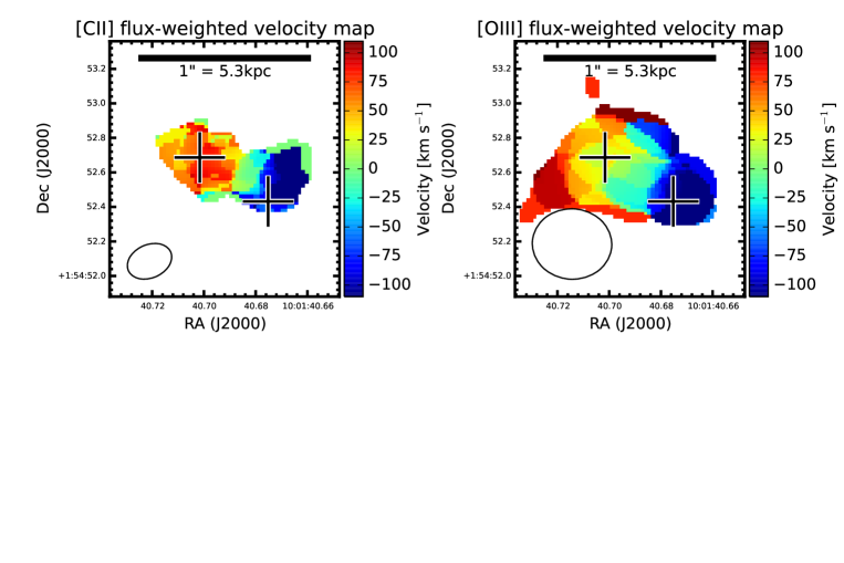
Figure 3: Left and right panels show flux-weighted velocity (i.e., Moment 1) maps of [Cii] and [Oiii] lines, respectively. The velocity zero point is defined as the systemic redshift, $z_{\rm sys}$ $=$ 7.1520. Only pixels with detections above $3\sigma$ are used to create the maps. The flux peak positions of the UV clumps are indicated by the black crosses. In each panel, the ellipse at lower left indicates the synthesized beam size of ALMA.

Based on the $S/N$-weighted mean redshifts, the velocity offset of the two clumps is $177\pm 16$ km s^-1. To better understand the velocity field of B14-65666, we also create a flux-weighted velocity (i.e., Moment 1) map of [Cii] and [Oiii]  with the CASA task immoments. In this procedure, we only include pixels above $3\sigma$ in the velocity-integrated intensity image (c.f., Jones et al. 2017a). The left and right panels of Figure 3 demonstrate that [Cii] and [Oiii] shows an $\approx 200$ km s^-1 velocity gradient, respectively.

Finally, Figure 4 shows a higher spatial resolution image of [Cii] with Briggs weighting and a robust parameter $0.3$ (Table 2.2) . The clump A has extended disturbed morphology, while the clump B has compact morphology.

To summarize, B14-65666 has two clumps in UV, [Cii], and [Oiii] whose positions are consistent with each other. The spectra of [Cii] and [Oiii] can be decomposed into two Gaussians kinematically separated by $\approx 200$ km s^-1. The velocity field is not smooth, implying that the velocity field may not be due to a rotational disk (see similar discussion in Jones et al. 2017b). These results indicate that B14-65666 is a merger system, as first claimed by Bowler et al. (2017) (see §1). A further discussion in terms of merger is presented in §8.1. Finally, we note that even the individual clumps have the highest [Cii] and [Oiii] luminosities among star forming galaxies at $z>6$ ([Cii]: Carniani et al. 2018b and references therein, [Oiii]: Inoue et al. 2016; Laporte et al. 2017; Carniani et al. 2017; Hashimoto et al. 2018a; Tamura et al. 2018).

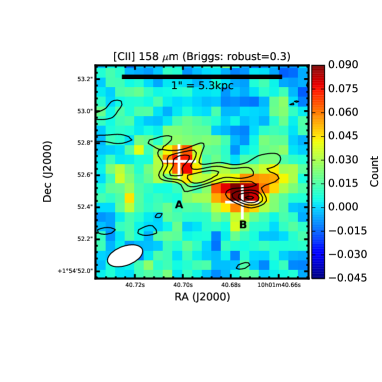
Figure 4: Zoomed-in [Cii] line image with a Briggs weighting (robust $=$ 0.3). Contours are drawn at ($-3$, $2$, $3$, $4$, $5$)$\times\sigma$, where $\sigma=26$ mJy beam^-1 km s^-1. White crosses show the positions of clumps A and B. The ellipse at lower left indicates the synthesized beam size of ALMA.

3.3 Dynamical Mass of the Individual Clumps

Assuming the virial theorem, we can derive the $M_{\rm dyn}$ value of the two individual clumps as

$$M_{\rm dyn.}=C\times\frac{r_{\rm 1/2}\sigma_{\rm line}^{2}}{G},$$ (2)

where $r_{\rm 1/2}$ is the half-light radius, $\sigma_{\rm line}$ is the line velocity dispersion, and $G$ is the gravitational constant. The factor $C$ depends on various effects such as the galaxy’s mass distribution, the velocity field along the line of sight, and relative contributions from random or rotational motions. For example, Binney & Tremaine (2008) shows that $C=$ 2.25 is an average value of known galactic mass distribution models. Erb et al. (2006) have used $C=$ 3.4 under the assumption of a disk geometry taking into account an average inclination angle of the disk. In the case of dispersion-dominated system, Förster Schreiber et al. (2009) have proposed that $C=$ 6.7 is appropriate for a variety of galaxy mass distributions. Because we do not see a clear velocity field in each clump (Figure 3), we use $C=$ 6.7. Adopting the major semi-axis of the 2D Gaussian fit for lines as $r_{\rm 1/2}$ (Table 3.1), we obtain $M_{\rm dyn}$ $=(5.7\pm 1.6)\times 10^{10}$ and ($3.1\pm 1.1)\times 10^{10}$ $M_{\rm\odot}$ for the clump A and B, respectively. Under the assumption that $M_{\rm dyn}$ of the whole system is the summation of the individual $M_{\rm dyn}$ values, we obtain the total dynamical mass of ($8.8\pm 1.9)\times 10^{10}$ $M_{\rm\odot}$. Note that our dynamical mass estimate is uncertain at least by a factor of three due to the uncertainty in $C$. Furthermore, given the nature of merger in B14-65666, the virial theorem may not be applicable for the individual clumps (and the whole system). Thus, our $M_{\rm dyn}$ values should be treated with caution. In §6, we compare the dynamical mass with the stellar mass derived from the SED fitting.

4 Dust

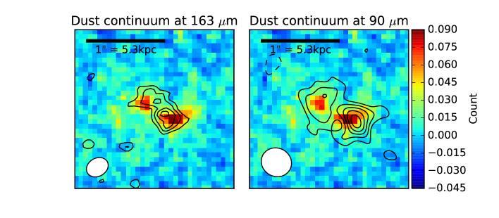
Figure 5: Left and right panels show ALMA dust continuum images overlaid on the $2^{\prime\prime}.0\times 2^{\prime\prime}.0$ cutout image of HST F140W, respectively. (Left) Dust continuum contours at $\approx 163$ $\mu$m drawn at ($-3$, $2$, $3$, $4$, $5$)$\times\sigma$, where $\sigma=9.5$ $\mu$Jy beam^-1. (Right) Dust continuum contours at $\approx 90$ $\mu$m drawn at (-3, 2, 3, 4, 5, 6)$\times\sigma$, where $\sigma=29.4$ $\mu$Jy beam^-1. In each panel, negative and positive contours are shown by the dashed and solid lines, respectively, and the ellipse at lower left indicates the synthesized beam size of ALMA.

We search for dust thermal emission in the two continuum images at around 163 and 90 . Hereafter, we refer to these two images as dust163 and dust90, respectively. The left and right panels of Figure 5 show contours of dust163 and dust90 overlaid on the HST F140W images, respectively, and our measurements are summarized in Table 3.1. We have detected a signal at the F140W position in the two images. We stress that B14-65666 is the second star-forming galaxy at $z>7$ after A1689$\_$zD1 (Watson et al. 2015; Knudsen et al. 2017) with dust continuum detections in multiple wavelengths. To obtain the continuum flux density of the individual clumps, we spatially integrate the image with the CASA task imfit assuming two-component 2D Gaussian profiles for the flux density. In this procedure, the positions of the 2D Gaussian components are fixed at the clump positions.

The clump A (B) has flux densities of $S_{\nu,163\mu m}=41\pm 23$ ($87\pm 26$) $\mu$Jy and $S_{\nu,90\mu m}=208\pm 83$ ($246\pm 73$) $\mu$Jy. Because the continuum emitting regions of the individual clumps are not spatially resolved, we adopt the beam size of dust163, i.e., the higher-angular resolution continuum image, as the upper limits. At $z=7.1520$, the upper limit of $0.29\times 0.23$ arcsec²corresponds to $1.6\times 1.2$ kpc².

For the whole system, the derived flux densities are $S_{\nu,163\mu m}=130\pm 25$ $\mu$Jy and $S_{\nu,90\mu m}=470\pm 128$ $\mu$Jy. The beam-deconvolved size of dust163 is $(0^{\prime\prime}.72\pm 0^{\prime\prime}.20)\times(0^{\prime\prime}.15\pm 0^{\prime\prime}.10)$, corresponding to $(3.8\pm 1.1)\times(0.8\pm 0.5)$ kpc² at $z=7.15$, with a positional angle (PA) of $46^{\circ}\pm 11^{\circ}$. Likewise, the beam-deconvolved size of dust90 is $(0^{\prime\prime}.80\pm 0^{\prime\prime}.25)\times(0^{\prime\prime}.40\pm 0^{\prime\prime}.16)$, corresponding to $(4.3\pm 1.4)\times(2.2\pm 0.9)$ kpc² at $z=7.15$, with PA $=57^{\circ}\pm 32^{\circ}$. These two size and PA values are consistent with each other within $1\sigma$ uncertainties. In Table 3.1, we only present the size of dust163 because it has a higher-angular resolution than dust90. At the current angular resolution of our data, it is possible that the continuum flux density of each clump is contaminated by the other clump. For accurate estimates, higher angular resolution data are required.

Our $S_{\nu,163\mu m}$ for the whole system is well consistent with the flux density at 158 $\mu$m presented by Bowler et al. (2018), $168\pm 56$ $\mu$Jy, taken at a lower angular resolution, further supporting our dust continuum detections. Bowler et al. (2018) have reported a spatial offset of $\Delta_{\rm tot.}=0^{\prime\prime}.60$ predominantly in the North-South direction ($\Delta_{\rm R.A.}=0^{\prime\prime}.17$, $\Delta_{\rm Dec.}=0^{\prime\prime}.57$) between their Band 6 dust continuum and F140W positions (see Figure 6 in Bowler et al. 2018). However, as shown in Figure 5, we do not find any significant spatial offset between our ALMA dust continuum and F140W positions although our F140W image has consistent astrometry with that of F140W image used in Bowler et al. (2018) (Appendix 1). Instead, based on comparisons of our and Bowler et al’s Band 6 data, we find a marginal ($2.3\sigma$) spatial offset of $\Delta_{\rm tot.}=0^{\prime\prime}.44$ between the two continuum images at the rest-frame wavelength of $\approx 160$  again predominantly in the North-South direction ($\Delta_{\rm R.A.}=0^{\prime\prime}.05$, $\Delta_{\rm Dec.}=0^{\prime\prime}.44$) (see Appendix 2 Figure 13). Although the origin of the possible spatial offset between the two ALMA Band 6 data is unclear, it would not be due to the resolved-out effect because the two Band 6 continuum flux densities are consistent within $1\sigma$ uncertainties.

We estimate the total infrared luminosity, $L_{\rm TIR}$, by integrating the modified black-body radiation over $8-1000$ . In star forming galaxies at $z>6-7$, all but one previous studies have assumed a dust temperature, $T_{\rm d}$, and a dust emissivity index, $\beta_{\rm d}$, because of none or a single dust continuum detection (e.g., Ota et al. 2014; Matthee et al. 2017; Laporte et al. 2017). The only one exception is A1689$\_$zD1 which has dust continuum detections at two wavelengths (Watson et al. 2015; Knudsen et al. 2017). In A1689$\_$zD1, Knudsen et al. (2017) have obtained $T_{\rm d}$ ranging from 36 K to 47 K under the assumption that $\beta_{\rm d}$ ranges from 2.0 to 1.5 with two dust continuum flux densities. Following analyses of Knudsen et al. (2017), we attempt to estimate $T_{\rm d}$ with fixed $\beta_{\rm d}$ values. For the whole system, correcting for the cosmic microwave background (CMB) effects (da Cunha et al. 2013; Ota et al. 2014), we obtain the best-fit $T_{\rm d}$ values of 61 K, 54 K, and 48 K for $\beta_{\rm d}=$ 1.5, 1.75, and 2.0, respectively, where the $1\sigma$ temperature uncertainty is about 10 K for each case. Because of loose constrains on $T_{\rm d}$ for the individual clumps, we assume the same combinations of $\beta_{\rm d}$ and $T_{\rm d}$ as in the whole system. We obtain $L_{\rm TIR}$ $\approx 1\times 10^{12}$, $3\times 10^{11}$, and $7\times 10^{11}$ $L_{\rm\odot}$, for the whole system, clump A, and clump B, respectively (Table 3.1). Owning to the two dust continuum detections, the $L_{\rm TIR}$ value is relatively well constrained in B14-65666.

Assuming a dust mass absorption coefficient $\kappa=\kappa_{0}(\nu/\nu_{0})^{\beta_{\rm d}}$, where $\kappa_{0}=10$ cm² g^-1 at $250$ $\mu$m (Hildebrand 1983), we obtain the dust mass, $M_{\rm d}$ $\approx 1\times 10^{7}$, $3\times 10^{6}$, and $6\times 10^{6}$ $M_{\rm\odot}$, for the whole system, clump A, and clump B, respectively (Table 3.1). We note that the dust mass estimate is in general highly uncertain due to the unknown $\kappa_{0}$ value. For example, if we use $\kappa_{0}=0.77$ cm² g^-1 at $850$ $\mu$m (Dunne et al. 2000), the dust mass estimates become twice as large.

5 Luminosity Ratios

5.1 IR-to-UV luminosity ratio (IRX) and IRX-$\beta$ relation

The ALMA spectroscopic literature sample: UV continuum slopes Name Redshift Waveband1 Waveband2 $\lambda_{\rm rest}$ $\beta$ $L_{\rm UV}$ $\mu$ (1) (2) (3) (4) (5) (6) (7) (8) (Å) ($10^{10}$$L_{\rm\odot}$) MACS1149-JD1 9.11 F140W $=25.88\pm 0.02$ F160W $=25.70\pm 0.01$ $1400-1600$ $-0.76\pm 0.16$ $(8.6\pm 0.2)/\mu$ 10 A2744$\_$YD4 8.38 F140W $=26.46\pm 0.04$ F160W $=26.42\pm 0.04$ $1500-1700$ $-1.63\pm 0.53$ $(4.5\pm 0.2)/\mu$ $1.8\pm 0.3$ MACS0416$\_$Y1 8.31 F140W $=26.08\pm 0.05$ F160W $=26.04\pm 0.05$ $1500-1700$ $-1.72\pm 0.50$ $(6.3\pm 0.3)/\mu$ $1.4$ A1689$\_$zD1 7.5 F140W $=24.64\pm 0.05$ F160W $=24.51\pm 0.11$ $1600-1900$ $-1.10\pm 0.83$ $(20.5\pm 0.9)/\mu$ 9.3 SXDF-NB1006-2 7.21 $J=25.46\pm 0.18$ $H>25.64$ $1500-1900$ $<-2.6$ $9.1\pm 1.5$ $-$ B14-65666 7.15 $J=24.7^{+0.2}_{-0.2}$ $H=24.6^{+0.3}_{-0.2}$ $1500-1900$ $-1.85^{+0.54}_{-0.53}$ ^a $19.9\pm 3.4$ $-$ IOK-1 6.96 F125W $=25.42\pm 0.05$ F160W $=25.44\pm 0.06$ $1600-2000$ $-2.07\pm 0.26$ $9.0\pm 0.4$ $-$ SPT0311-58E 6.90 F125W $=25.28\pm 0.10$ F160W $=24.98\pm 0.12$ $1600-2000$ $-0.88\pm 0.58$ $(10.1\pm 0.9)/\mu$ $1.3$ COS-3018555981 6.85 F125W $-^{b}$ F160W $-^{b}$ $1600-2000$ $-1.22\pm 0.51$ $11\pm 1^{c}$ $-$ COS-2987030247 6.81 F125W $-^{b}$ F160W $-^{b}$ $1600-2000$ $-1.18\pm 0.53$ $13\pm 1^{c}$ $-$ Himiko 6.60 F125W $=24.99\pm 0.08$ F160W $=24.99\pm 0.10$ $1600-2100$ $-2.00\pm 0.48$ $12.4\pm 1.1$ $-$ Note. (1) Object Name; (2) Spectroscopic redshift; (3) and (4) Two wavebands and their photometry values to derive the UV continuum slope; (5) Rest-frame wavelength range probed by the wavebands; (6) UV spectral slope; (7) UV luminosity at $\approx 1500$ Å obtained from the photometry value of the Waveband1; and (8) lensing magnification factor. Upper limits represent $3\sigma$.
Redshift and photometry values are taken from the literature as summarized below.
MACS1149-JD1: Redshift (Hashimoto et al. 2018a); F140W and F160W (Zheng et al. 2017);
A2744$\_$YD4: Redshift (Laporte et al. 2017); F140W and F160W (Zheng et al. 2014);
MACS0416$\_$Y1: Redshift (Tamura et al. 2018); F140W and F160W (Laporte et al. 2015);
A1689$\_$zD1: Redshift (Watson et al. 2015); F125W and F160W (Watson et al. 2015);
SXDF-NB1006-2: Redshift (Inoue et al. 2016); $J$ and $H$ (Inoue et al. 2016);
B14-65666: Redshift (This Study); $J$ and $H$ (Bowler et al. 2014);
IOK-1: Redshift (Ota et al. 2014); F125W and F160W (Jiang et al. 2013; the object No. 62 in their Table 1);
SPT0311-058E: Redshift (Marrone et al. 2018); F125W and F160W (Marrone et al. 2018);
COS-3018555981: Redshift (Smit et al. 2018);
COS-2987030247: Redshift (Smit et al. 2018);
Himiko: Redshift (Ouchi et al. 2013); F125W and F160W (Ouchi et al. 2013)
^a The UV spectral slope in Bowler et al. (2018) based on the updated photometry values.
^b Not available.
^c Values taken from Smit et al. (2018).

The ALMA spectroscopic literature sample: Infrared-excess (IRX) Name $S_{\rm\nu}$ Rest-Wavelength $L_{\rm TIR}$ IRX Ref. ($\mu$Jy) ($\mu$m) ($10^{10}$$L_{\rm\odot}$) (1) (2) (3) (4) (5) (6) MACS1149-JD1 $<53/\mu$ 90 $<11.4/\mu$ $<0.12$ Hashimoto et al. (2018a) A2744$\_$YD4 $(175\pm 69)/\mu^{a}$ 90 $(32.7\pm 12.9)/\mu$ $0.86\pm 0.22$ Laporte et al. (2017) MACS0416$\_$Y1 $(137\pm 26)/\mu$ 91 $(25.7\pm 4.9)/\mu$ $0.61\pm 0.09$ Tamura et al. (2018) A1689$\_$zD1 $(1330\pm 140)/\mu$ 103 $(255\pm 26.8)/\mu$ $1.09\pm 0.05$ Knudsen et al. (2017) SXDF-NB1006-2 $<42$ 162 $<19.6$ $<0.33$ Inoue et al. (2016) B14-65666 $130\pm 25$ 163 $61.8\pm 11.9$ $0.49\pm 0.12$ Bowler et al. (2018), This Study IOK-1 $<63$ 162 $<28.0$ $<0.49$ Ota et al. (2014) SPT0311-E $(1530\pm 70)/\mu$^b 159 $(640\pm 30)/\mu$ $1.80\pm 0.04$ Marrone et al. (2018) COS-3018555981 $<87$ 158 $<35.4$ $<0.51$ Smit et al. (2018) COS-2987030247 $<75$ 158 $<30.2$ $<0.37$ Smit et al. (2018) Himiko $<51$ 153 $<18.0$ $<0.16$ Ouchi et al. (2013) Note. (1) Object Name; (2) and (3) Dust continuum flux density and its rest-frame wavelength; (4) Total IR luminosities estimated by integrating the modified-black body radiation at $8-1000$ $\mu$m with $T_{\rm d}=$ 50 K and $\beta_{\rm d}=1.5$; (5) IRX values with $T_{\rm d}=$ 50 K and $\beta_{\rm d}=1.5$; and (6) Reference. Upper limits represent $3\sigma$.
^a Continuum flux density after performing primary beam correction.
^b Continuum flux density before the lensing correction is estimated from the intrinsic flux density of $1.18\pm 0.05$ mJy and $\mu=1.3$ (Marrone et al. 2018).

The relation between the IR-to-UV luminosity ratio, IRX$\equiv$ log₁₀($L_{\rm TIR}$/$L_{\rm UV}$), and the UV continuum slope, $\beta$, is useful to constrain the dust attenuation curve of galaxies (e.g., Meurer et al. 1999). Local starburst galaxies are known to follow the Calzetti’s curve (e.g., Calzetti et al. 2000; Takeuchi et al. 2012). Studies have shown that high-$z$ galaxies may favor a steep attenuation curve similar to that of the Small Magellanic Could (SMC) (e.g., Reddy et al. 2006; Kusakabe et al. 2015). Based on a stacking analysis of LBGs at $z\approx 2-10$, Bouwens et al. (2016) show that high-$z$ galaxies have a low IRX value at a given $\beta$, even lower than the SMC curve. This is interpreted as a steep attenuation curve or a high $T_{\rm d}$ at high-$z$, the latter being supported from detailed analyses of the IR spectral energy distribution in high-$z$ analogs (Faisst et al. 2017, see also Behrens et al. 2018). On the other hand, several studies claim that there is no or little redshift evolution in the IRX-$\beta$ relation at least up to $z\approx 5$ (Fudamoto et al. 2017; Koprowski et al. 2018). Thus, a consensus is yet to be reached on the high-$z$ IRX-$\beta$ relation.

At $z\gtrsim 6$, little is understood about the IRX-$\beta$ relation due to the small sample with dust continuum detections (Bowler et al. 2018). Therefore, B14-65666 would provide us with a clue to understand the IRX-$\beta$ relation at $z>6$. Bowler et al. (2018) have first discussed the position of B14-65666 in the IRX-$\beta$ relation. The authors have compared the whole system of B14-65666 with the $z\approx 3-5$ results (Fudamoto et al. 2017; Koprowski et al. 2018), a stacking result of $z\approx 4-10$ (Bouwens et al. 2016), and with another $z>7$ galaxy that has a dust continuum detection, A1689$\_$zD1 (Watson et al. 2015; Knudsen et al. 2017).

In this study, we focus on the IRX-$\beta$ relation at $z>6.5$ based on a compiled sample of eleven spectroscopically confirmed galaxies. Tables 5.1 and 5.1 summarize our sample from the literature and this study. The sample includes five galaxies with dust continuum detections: A1689$\_$zD1 (Watson et al. 2015; Knudsen et al. 2017), A2744$\_$YD4 (Laporte et al. 2017), MACS0416$\_$Y1 (Tamura et al. 2018), SPT0311-58E (Marrone et al. 2018), and B14-65666 (see also Bowler et al. 2018). In addition, the sample includes objects with deep $3\sigma$ upper limits on the IRX obtained with ALMA: Himiko (Ouchi et al. 2013; Schaerer et al. 2015), IOK-1 (Ota et al. 2014; Schaerer et al. 2015), SXDF-NB1006-2 (Inoue et al. 2016), COS-301855981, COS-29870300247 (Smit et al. 2018), and MACS1149-JD1 (Hashimoto et al. 2018a).

For fair comparisons of the data points, we uniformly derive $\beta$ from two photometry values following the equation (1) of Ono et al. (2010). We use the combination of (F125W, F160W) and (F140W, F160W) or ($J$, $H$) at two redshift bins of $z=6.60-7.21$ and $z=7.5-9.11$, respectively. These wavebands probe the rest-frame wavelength ranges of $\approx 1600-2000$ Å and $1500-1700$ Å at the two redshift bins. Because of the difference in the probed wavelength range, the derived $\beta$ values should be treated with caution. The estimated $\beta$ values are summarized in Table 5.1. To estimate the UV luminosity, $L_{\rm UV}$, of the sample, we consistently use the rest-frame $\approx 1500$ Å magnitude of the waveband1 in Table 5.1. To obtain $L_{\rm TIR}$ of the literature sample, we have assumed $T_{\rm d}$ $=50$ K and $\beta_{\rm d}=1.5$. These assumptions would be reasonable because A1689$\_$zD1 and B14-65666 have $T_{\rm d}$ $\approx 40-60$ K at $\beta_{\rm d}=2.0-1.5$ (see §4).

In B14-65666, because only one HST photometry data point (F140W) is available, we cannot obtain $\beta$ of the individual clumps. Therefore, we investigate the IRX and $\beta$ values of the entire system. We adopt $\beta=-1.85^{+0.54}_{-0.53}$ in Bowler et al. (2018) calculated with updated $J$- and $H$-band photometry values. For fair comparisons to other data points, we assume $T_{\rm d}$ $=$ 50 K and $\beta_{\rm d}=1.5$ to obtain $L_{\rm TIR}$ $=(6.2\pm 1.2)\times 10^{11}$ $L_{\rm\odot}$, which is about a factor two lower than the values presented in Table 3.1. With $L_{\rm UV}=2.0\times 10^{11}$ $L_{\rm\odot}$, we obtain the IRX value of $0.5\pm 0.1$. If we instead use the $L_{\rm TIR}$ values in Table 3.1, we obtain a slightly higher IRX value, $0.7\pm 0.1$. Therefore, we adopt IRX $=0.5^{+0.3}_{-0.1}$ as a fiducial value.

Figure 6 shows the $z>6.5$ galaxies in the IRX-$\beta$ relation. We also plot the IRX-$\beta$ relations based on the Calzetti and SMC dust laws assuming the intrinsic $\beta$ value of $-2.2$ (Bouwens et al. 2016). We find that five LBGs with dust continuum detections are consistent with the Calzetti’s curve if we assume $T_{\rm d}$ $=50$ K and $\beta_{\rm d}=1.5$. Among the six null-detections, SXDF-NB1006-2 has a very steep UV slope $\beta<-2.6$ ($3\sigma$). Such a steep $\beta$ can be reproduced if we assume a very young stellar age ($<10$ Myr) or low metallicity (e.g., Schaerer 2003; Bouwens et al. 2010, see also Figure 10 of Hashimoto et al. 2017a). Likewise, MACS1149-JD1 has a stringent upper limit on the IRX value. Although it is possible that MACS1149-JD1 lies below the SMC curve, we note that the presented $\beta$ value of MACS1149-JD1 probes the rest-frame wavelength range of $1400-1600$ Å. Deeper $K$ band data would allow us to compute $\beta$ in the wavelength range of $\approx 1500-2200$ Å which is comparable to that probed in previous high-$z$ studies (e.g., Bouwens et al. 2009; Hashimoto et al. 2017b).

Although a large and uniform sample with dust continuum detections is needed to understand the typical attenuation curve at $z>6.5$, our first results show that there is no strong evidence for a steep (i.e., SMC-like) attenuation curve at least for the five LBGs detected in dust.

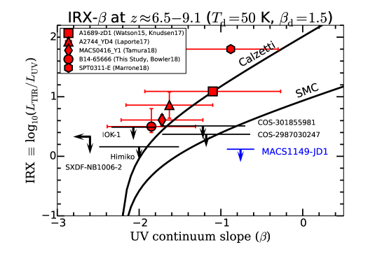
Figure 6: The IRX, plotted against the UV slope, $\beta$, for eleven spectroscopically identified galaxies at $z\approx 6.5-9.1$. For fair comparisons of data points from the literature, we have uniformly derived $\beta$ and IRX values (see §5.1 for the details). We plot the IRX value under the assumption of $T_{\rm d}$ $=50$ K and $\beta_{\rm d}=1.5$. The arrows correspond to $3\sigma$ upper limits. In each panel, the two solid black lines indicate the IRX-$\beta$ relation based on the Calzetti and SMC dust laws (Bouwens et al. 2016). The five red symbols denote objects with dust continuum detections; A1689$\_$zD1 (Watson et al. 2015; Knudsen et al. 2017), A2744$\_$YD4 (Laporte et al. 2017), MACS0416$\_$Y1 (Tamura et al. 2018), SPT0311-58E (Marrone et al. 2018), and B14-65666. The details of the data are summarized in Tables 5.1 and 5.1.

5.2 [Oiii]/[Cii] Luminosity Ratio

The line luminosity ratio, [Oiii]/[Cii], would give us invaluable information on chemical and ionization properties of galaxies (e.g., Inoue et al. 2016; Marrone et al. 2018). For example, in local galaxies, a number of studies have examined the line ratio (Malhotra et al. 2001; Brauher et al. 2008; Madden et al. 2012; Cormier et al. 2015). These studies have shown that dwarf metal-poor galaxies have high line ratios, [Oiii]/[Cii] $\approx 2-10$, whereas metal-rich galaxies have low line ratios, [Oiii]/[Cii] $\approx 0.5$. Alternatively, if the ISM of galaxies is highly ionized, the [Cii] luminosity would be weak because [Cii] emission is predominantly emitted from the PDR (e.g., Vallini et al. 2015; Katz et al. 2017).

In B14-65666, the line luminosity ratio is [Oiii]/[Cii] $=3.1\pm 0.6$, $3.5\pm 0.8$, $2.7\pm 0.6$ for the whole system, clump A, and clump B, respectively (Table 3.1). We compare our results with those in other high-$z$ galaxies in the literature: two $z\approx 7$ star-forming galaxies and two $z\approx 6-7$ sub-millimeter galaxies (SMGs). Inoue et al. (2016) have detected [Oiii] from a $z=7.21$ LAE with the EW₀(Ly$\alpha$)  value of 33 Å (SXDF-NB1006-2: Shibuya et al. 2012). With the null detection of [Cii], the authors have shown that SXDF-NB1006-2 has a total line luminosity ratio of [Oiii]/[Cii] $>12$ ($3\sigma$). Carniani et al. (2017) have reported detections of [Oiii] and [Cii] in a galaxy at $z=7.11$ (BDF-3299: Vanzella et al. 2011; Maiolino et al. 2015). BDF-3299 has a large EW₀(Ly$\alpha$) $=50$ Å and thus can be categorized into LAEs. The galaxy has spatial offsets between [Oiii], [Cii], and UV emission. Under the assumption that both [Cii] and [Oiii] are associated with the UV emission, we obtain the total line ratio of $3.7\pm 0.6$ using the [Cii] luminosity ($4.9\pm 0.6\times 10^{8}$ $L_{\rm\odot}$) and the [Oiii] luminosity ($18\pm 2\times 10^{8}$ $L_{\rm\odot}$) . Recently, Marrone et al. (2018) have detected both [Oiii] and [Cii] from a lensed SMG at $z=6.90$ comprised of two galaxies (SPT0311-058E and SPT0311-058W). The total line luminosity ratio is $1.27\pm 0.18$ and $0.56\pm 0.17$ for SPT0311-058E and SPT0311-058W, respectively, where the $1\sigma$ values take the uncertainties on magnification factors into account. Finally, Walter et al. (2018) have detected [Oiii] in an SMG at $z=6.08$ located at the projected distance of $\approx 61$ kpc from a quasar at the same redshift. In the SMG, J2100-SB, the authors have presented the line luminosity ratio of $1.58\pm 0.24$ combining the previous [Cii] detection (Decarli et al. 2017).

Based on the combined sample of these literature objects with B14-65666, we investigate the relation between the line luminosity ratio and the bolometric luminosity estimated as $L_{\rm bol}\approx L_{\rm UV}+L_{\rm TIR}$. In B14-65666, we obtain $L_{\rm bol}=(12.5\pm 1.5)\times 10^{11}$, $(4.2\pm 0.5)\times 10^{11}$ and $(8.1\pm 1.0)\times 10^{11}L_{\rm\odot}$ for the whole system, clump A, and clump B, respectively (Table 3.1). For the two LAEs without dust continuum detections, we derive the upper limits of $L_{\rm bol}$ as the $L_{\rm UV}$ measurements plus the $3\sigma$ upper limits of $L_{\rm TIR}$, where we assume $T_{\rm d}$ $=$ 50 K and $\beta_{\rm d}=1.5$. The $L_{\rm UV}$ value is used as lower limits of $L_{\rm bol}$ . The $L_{\rm TIR}$ value of the two SMGs are well constrained from multiple dust continuum detections at different wavelengths (see Extended Data Figure 7 in Marrone et al. 2018). Because these SMGs have $L_{\rm UV}$/$L_{\rm TIR}$ $\approx 0.002-0.02$, we assume $L_{\rm bol}\approx$ $L_{\rm TIR}$ for these objects. We thus adopt $L_{\rm bol}=(4.6\pm 1.2)\times 10^{12}$ and $(3.3\pm 0.7)\times 10^{13}L_{\rm\odot}$ for SPT0311-58E and SPT0311-58W, respectively. Similarly, because J2100-SB is not detected in the rest-frame UV/optical wavelengths, we assume $L_{\rm bol}\approx$ $L_{\rm TIR}$ $=(1.9\pm 0.03)\times 10^{12}$ $L_{\rm\odot}$ (Walter et al. 2018).

Figure 7 shows a clear anti-correlation, although a larger number of galaxies are needed for a definitive conclusion. Given that the bolometric luminosity traces the mass scale of a galaxy (i.e., the stellar and dark matter halo masses and/or the SFR), the possible trend implies that lower mass galaxies having higher luminosity ratios. These would in turn indicate that lower mass galaxies have lower metallicity and/or higher ionization states (cf., Maiolino & Mannucci 2019; Nakajima et al. 2016). Because we do not have direct measurements of these parameters in the sample, we leave further discussion to future studies.

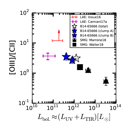
Figure 7: [Oiii]-to-[Cii] line luminosity ratio plotted against the bolometric luminosity estimated as the summation of the UV and IR luminosities for $z\approx 6-7$ objects. The red arrow represents the $3\sigma$ lower limit of the line luminosity ratio in the LAE of Inoue et al. (2016). For the two LAEs without $L_{\rm TIR}$ measurements, the upper limits of $L_{\rm bol.}$ are estimated as the summation of $L_{\rm UV}$ and the $3\sigma$ upper limits on $L_{\rm TIR}$, where we assume $T_{\rm d}$ $=$ 50 K and $\beta_{\rm d}=1.5$. The lower limits of $L_{\rm bol.}$ for the two LAEs correspond to $L_{\rm UV}$. Detailed calculations of these values are presented in §5.2.

6 SED fit

We perform stellar population synthesis model fitting to B14-65666 to derive the stellar mass ($M_{\rm*}$), dust attenuation ($A_{\rm V}$), the stellar age, stellar metallicity ($Z$), and the SFR.

We use the $Y$, $J$, $H$, and $K$ band data taken by UltraVISTA (Bowler et al. 2014) and the deep Spitzer/IRAC 3.6 and 4.5 $\mu$m data (Bowler et al. 2017). The clumps A and B are not resolved under the coarse angular resolution of ground based telescopes. Therefore, the photometry values represent the total system of B14-65666. We thus perform SED fitting to the total system. In addition, we use our dust continuum flux densities and the [Oiii] flux. We do not use the [Cii] flux. This is due to the difficulty in modeling [Cii] which arises both from the HII region and the PDR (see Inoue et al. 2014b).

The SED fitting code used in this study is the same as that used in Hashimoto et al. (2018a) and Tamura et al. (2018). For the detailed procedure, we refer the reader to Mawatari et al. (2016) and the relevant link . Briefly, the stellar population synthesis model of GALAXEV (Bruzual & Charlot 2003) is used. The nebular continuum and emission lines of Inoue (2011a) are included. The [Oiii] line flux is estimated based on metallicity and the SFR with semi-empirical models (Inoue et al. 2014b, 2016). A Calzetti’s law (Calzetti et al. 2000) is assumed for dust attenuation, which is appropriate for B14-65666 based on the results of the IRX-$\beta$ relation (§5.1). The same attenuation value is used for the stellar and nebular components (e.g., Erb et al. 2006; Kashino et al. 2013). An empirical dust emission templates of Rieke et al. (2009) is adopted. The Chabrier initial mass function (Chabrier 2003) with $0.1-100$ $M_{\rm\odot}$ is adopted, and a mean IGM model of Inoue et al. (2014a) is applied. We fix the object’s redshift of $7.1520$. To estimate the best-fit parameters, we use the least $\chi^{2}$ formula of Sawicki (2012) including an analytic treatment of upper limits for non-detections. Uncertainties on the parameters are estimated based on a Monte Carlo technique ($N=300$).

For simplicity, we assume a constant star formation history (SFH). Figure 8 shows the best-fit SED of B14-65666 and Table 6 summarize the estimated physical quantities. The strong [Oiii] line flux indicates a very high current SFR, $200^{+82}_{-38}$ $M_{\rm\odot}$ yr^-1. We note that our stellar mass, $M_{\rm*}=7.7^{+1.0}_{-0.7}\times 10^{8}$ $M_{\rm\odot}$, or log($M_{\rm*}/M_{\rm\odot})=8.9\pm 0.1$, and the dust extinction value, $A_{\rm V}=0.3^{+0.19}_{-0.10}$, are consistent with the results of Bowler et al. (2014, 2018) within $1\sigma$ uncertainties. In §8.1, we use the SED-fitting results to discuss the properties of B14-65666.

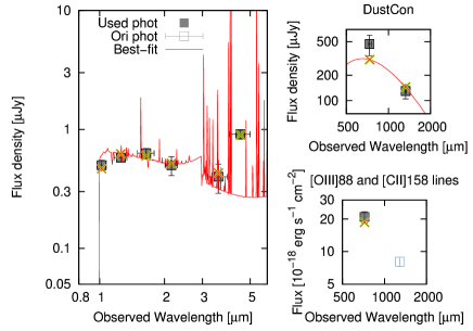
Figure 8: Best-fit SED (left) taking into account the dust continuum flux densities (top right) and the [Oiii] flux (bottom right) for a constant star-formation model. In the left panel, black squares show $Y,J,H,K$-band photometry and the IRAC channel 1 and 2 measurements, from left to right. An open-white square (’Ori phot’) indicates the photometric data point of [Cii] 158 , which is not used in the SED fitting (see the text for the details). Horizontal and vertical error bars represent the wavelength range of the filters and the $1\sigma$ uncertainties, respectively. The red solid line indicates the SED model and the corresponding band flux densities are shown by crosses. In the top right panel, the black squares are the dust continuum flux densities at 90 and 163  and their $1\sigma$ uncertainties. In the bottom right panel, the black square shows the observed [Oiii] flux and its $1\sigma$ uncertainty, while the cross is the model prediction.

Results of SED fit Parameters Values $\chi^{2}$ 4.30 $\nu$ 4 A_V [mag] $0.30^{+0.19}_{-0.10}$ Age [Myr] $3.8^{+1.8}_{-1.3}$ Metallicity $0.008^{+0.008}_{-0.004}$ Escape fraction $0.0^{+0.2}_{-0.0}$ Stellar mass ($M_{\rm\odot}$) [$10^{8}$ M_⊙] $7.7^{+1.0}_{-0.7}$ SFR [M_⊙ yr^-1] $200^{+82}_{-38}$ Note. The stellar mass and SFR values are obtained with the Chabrier IMF with $0.1-100$ $M_{\rm\odot}$. The solar metallicity corresponds to 0.02. Because we have nine data points (Figure 8) and attempt to constrain five parameters, the degree of freedom, $\nu$, is four. Note that the SFR value is not a variable parameter because SFR is readily obtained from the stellar age and stellar mass under the assumption of a star formation history.

To test the validity of our SED-fit results, we examine if the derived stellar and dust masses can be explained in a consistent manner. Based on a combination of the stellar mass of $\approx 7.7\times 10^{8}$ $M_{\rm\odot}$ and the effective number of supernovae (SN) per unit stellar mass in the Chabrier IMF, 0.0159 $M_{\rm\odot}$^-1 (e.g., Inoue 2011b), we obtain the number of SN $\approx 1.2\times 10^{7}$. Thus, the dust mass of $\approx 1\times 10^{7}$ $M_{\rm\odot}$ requires the dust yield per SN $\approx 0.8$ $M_{\rm\odot}$, which can be achieved if the dust destruction is insignificant (e.g., Michałowski 2015). The dust-to-stellar mass ratio, log($M_{\rm*}/M_{\rm d})\approx$ -1.9, is high but within the range observed in local galaxies (see Figure 11 in Rémy-Ruyer et al. 2015) and can be explained by theoretical models (Popping et al. 2017; Calura et al. 2017).

Finally, we compare the stellar mass with the dynamical mass (§3.3). The derived stellar mass, $M_{\rm*}=7.7^{+1.0}_{-0.7}\times 10^{8}$ $M_{\rm\odot}$, is well below $M_{\rm dyn}$ $=(8.8\pm 1.9)\times 10^{10}$ $M_{\rm\odot}$. The dynamical-to-stellar mass ratio, log($M_{\rm dyn}/M_{\rm*}$) $\approx 2.0$, is high but within the range obtained in star-forming galaxies at $z\approx 2-3$ (e.g., Erb et al. 2006; Gnerucci et al. 2011).

One might think that the stellar age ($\approx 4$ Myr) seems too young to reproduce the dust mass. However, we note that the stellar age deduced from the SED fitting indicates the age after the onset of current star formation activity. Given the signature of merger activity, we could infer the existence of star formation activity well before the observing timing at $z=7.15$ which forms two galaxies and a significant fraction of the dust mass (see such an example in Tamura et al. 2018).

7 Ly$\alpha$ velocity offset

Because Ly$\alpha$ is a resonant line, it is known that the Ly$\alpha$ redshift, $z_{\rm Ly\alpha}$, does not exactly match the systemic redshift defined by optically-thin nebular emission lines, e.g., [Oiii] and [Cii]. The discrepancy between the two redshifts provides a valuable probe of the interstellar medium (ISM) and the surrounding intergalactic medium (IGM). For example, based on radiative transfer calculations, theoretical studies (Dijkstra et al. 2006; Verhamme et al. 2006, 2015; Gronke et al. 2015) predict that the Ly$\alpha$ line is redshifted (blueshifted) with respect to the systemic redshift if a galaxy has an outflowing (inflowing) gas in the ISM. When Ly$\alpha$ photons enter the IGM, its spectral profile is further altered due to the damping wing of Ly$\alpha$ absorption by the intergalactic neutral hydrogen, increasing $z_{\rm Ly\alpha}$ (Haiman 2002; Laursen et al. 2013).

We measure the velocity offset of the Ly$\alpha$ line calculated as

$$\Delta v_{\rm Ly\alpha}=c\times\frac{z_{\rm Ly\alpha}-z_{\rm sys}}{1+z_{\rm sys}},$$ (3)

where $c$ is the speed of light. We have remeasured $z_{\rm Ly\alpha}$ in the spectrum of Furusawa et al. (2016) by reading the peak wavelength of a Gaussian fit to the line, taking into account air refraction and the motion of the observatory. With the vacuum rest-frame wavelength of $1215.67$ Å, we have obtained $z_{\rm Ly\alpha}$$=7.1730\pm 0.0012$ in the Solar system barycentric frame (Table 3.1). Thus, we obtain $\Delta v_{\rm Ly\alpha}$ $=772\pm 45$ km s^-1 (Figure 9). We note that the quality of our FOCAS spectrum is insufficient to determine the exact spatial position of Ly$\alpha$. Thus, we add a systematic uncertainty of $\pm 100$ km s^-1 to reflect the fact that B14-65666 is comprised of two clumps kinematically separated by $\approx 200$ km s^-1 (Figure 3). Hereafter we adopt $\Delta v_{\rm Ly\alpha}$ $=772\pm 45\pm 100$ km s^-1.

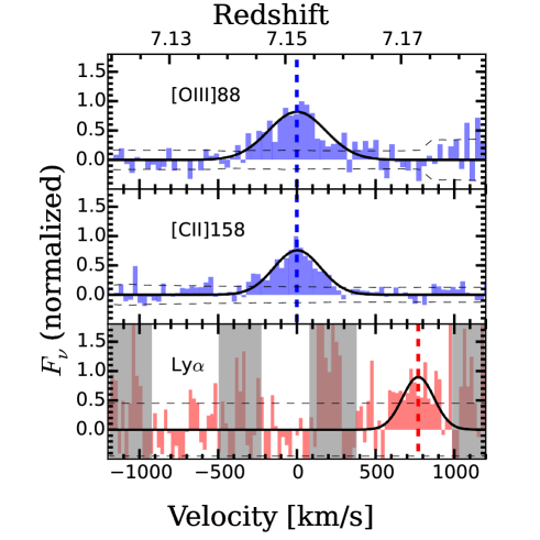
Figure 9: Top, middle, and bottom panel show ALMA [Oiii] 88 $\mu$m, ALMA [Cii] 158 $\mu$m, and Subaru/FOCAS Ly$\alpha$ spectra in velocity space with a resolution of $\sim 30$ km s^-1, $33$ km s^-1, and $25$ km s^-1, respectively. The velocity zero point corresponds to the systemic redshift $z=7.1520$ (blue dashed line) and the Ly$\alpha$ offset is $\simeq 770$ km s^-1 (red dashed line). Grey rectangles show regions contaminated by night sky emission. The black dashed lines indicate the RMS noise level for the velocity resolutions, and the black curves are Gaussian fit to the lines.

We compare the $\Delta v_{\rm Ly\alpha}$ value of B14-65666 with those in the literature. The Ly$\alpha$ velocity offsets are investigated in hundreds of galaxies at $z\approx 2-3$ where both Ly$\alpha$ and H$\alpha$ or [Oiii] 5007 Å are available (e.g., Steidel et al. 2010; Hashimoto et al. 2013, 2015; Erb et al. 2014; Shibuya et al. 2014). At $z\approx 2-3$, galaxies have velocity offsets ranging from 100 to 1000 km s^-1 with a mean value of $200-400$ km s^-1 (e.g., Erb et al. 2014; Trainor et al. 2015; Nakajima et al. 2018). At $z>6$, there are 16 galaxies whose $\Delta v_{\rm Ly\alpha}$ values are measured. The systemic redshifts of these galaxies are based on either [Cii] 158  and [Oiii] 88  (Willott et al. 2015; Knudsen et al. 2016; Inoue et al. 2016; Pentericci et al. 2016; Bradač et al. 2017; Carniani et al. 2017, 2018a; Laporte et al. 2017; Matthee et al. 2017) or rest-frame UV emission lines such as CIII]1909 Å and OIII]1666 Å (Stark et al. 2015b, 2017; Mainali et al. 2017; Verhamme et al. 2018). At $z\approx 6-8$, velocity offsets of $100-500$ km s^-1 are reported. We summarize these literature sample at $z\approx 6-8$ in Table 7. Compared with these literature values, the $\Delta v_{\rm Ly\alpha}$ value of B14-65666 is the largest at $z\approx 6-8$, and even larger than the typical $\Delta v_{\rm Ly\alpha}$ value at $z\approx 2-3$.

From the point of view of Ly$\alpha$ radiative transfer in expanding shell models, there are two possible interpretations of a large $\Delta v_{\rm Ly\alpha}$ value. The first interpretation is that a galaxy has a large neutral hydrogen column density, $N_{\rm HI}$, in the ISM. In the case of large $N_{\rm HI}$, the number of resonant scattering of Ly$\alpha$ photons becomes large, which in turn increases the $\Delta v_{\rm Ly\alpha}$ value (e.g., Verhamme et al. 2015). In this case, EW₀(Ly$\alpha$) becomes small because Ly$\alpha$ photons suffer from more dust attenuation due to a larger optical path length. Such a trend is confirmed at $z\approx 2-3$, where larger $\Delta v_{\rm Ly\alpha}$ values are found in galaxies with brighter $M_{\rm UV}$ (hence larger $N_{\rm HI}$; Garel et al. 2012) and smaller EW₀(Ly$\alpha$) (e.g., Hashimoto et al. 2013; Shibuya et al. 2014; Erb et al. 2014). However, it is unclear if such a trend is also true at $z>6$. The second interpretation is that a galaxy has a large outflow velocity, $v_{\rm out}$. Because Ly$\alpha$ photons scattered backward of receding gas from the observer preferentially escape from the galaxy, the Ly$\alpha$ velocity offset is positively correlate with the outflow velocity as $\Delta v_{\rm Ly\alpha}$ $\sim 2\times v_{\rm out}$ (e.g., Verhamme et al. 2006).

To investigate the two scenarios, we explore correlations between $\Delta v_{\rm Ly\alpha}$, EW₀(Ly$\alpha$), and $M_{\rm UV}$ at $z\approx 6-8$ based on 17 galaxies in Table 7. In addition, we also investigate the relation between $\Delta v_{\rm Ly\alpha}$ and [Cii] luminosities for the first time. Figure 10 shows $\Delta v_{\rm Ly\alpha}$ values plotted against EW₀(Ly$\alpha$), $M_{\rm UV}$, and [Cii] luminosities. To evaluate the significance of the relation, we perform Spearman rank correlation tests.

In the left panel of Figure 10, the correlation is weak with a Spearman rank correlation coefficient of $p=0.37$. In the left panel of Figure 11, we compare our $\Delta v_{\rm Ly\alpha}$ values at $z\approx 6-8$ with those at $z\approx 2-3$ (Erb et al. 2014; Nakajima et al. 2018). At $z\approx 2-3$, Erb et al. (2014) have reported a $7\sigma$ anti-correlation. It is possible that the correlation at $z\approx 6-8$ is diluted because both $\Delta v_{\rm Ly\alpha}$ and EW₀(Ly$\alpha$) values are affected by the IGM attenuation effect. A large number of objects with $\Delta v_{\rm Ly\alpha}$ measurements, particularly those with large EW₀(Ly$\alpha$) values, are needed to conclude if the correlation exists or not at $z\gtrsim 6$. Nevertheless, we note that the scatter of $\Delta v_{\rm Ly\alpha}$ value becomes larger for smaller EW₀(Ly$\alpha$) galaxies. Such a trend is consistent with results at $z\approx 2-3$, as shown in the left panel of Figure 11. In the middle panel of Figure 10, we confirm a $4.5\sigma$ correlation between $M_{\rm UV}$ and $\Delta v_{\rm Ly\alpha}$, indicating that brighter $M_{\rm UV}$ objects have larger $\Delta v_{\rm Ly\alpha}$. Although the trend is consistent with that at $z\approx 2-3$ (right panel of Figure 11), we have identified the trend at $z\approx 6-8$ for the first time. In the right panel of Figure 10, we identify a positive correlation at the significance level of $4.0\sigma$, indicating that galaxies with higher [Cii] luminosities have larger $\Delta v_{\rm Ly\alpha}$ values.

The correlations in the middle and right panels of Figure 10 support the two aforementioned scenarios for the large $\Delta v_{\rm Ly\alpha}$ in B14-65666. In the $N_{\rm HI}$ scenario where we interpret $\Delta v_{\rm Ly\alpha}$ as $N_{\rm HI}$, the middle panel of Figure 10 indicates that UV brighter objects have larger $N_{\rm HI}$. This is consistent with the results of semi-analytical models implementing the Ly$\alpha$ radiative transfer calculations (Garel et al. 2012; see their Figure 12). In this scenario, the right panel of Figure 10 indicates that higher [Cii] luminosity objects have larger $N_{\rm HI}$. Such a trend is indeed confirmed in our Galaxy and some nearby galaxies (e.g., Bock et al. 1993; Matsuhara et al. 1997).

In the outflow scenario where we translate $\Delta v_{\rm Ly\alpha}$ as the outflow velocity, given the correlation between the SFR and the [Cii] luminosity (e.g., De Looze et al. 2014; Matthee et al. 2017; Carniani et al. 2018b; Herrera-Camus et al. 2018) or the UV luminosity, the middle and right panels of Figure 10 show that larger SFR objects have stronger outflows. This is consistent with the observational results in the local Universe (e.g., Martin 2005; Weiner et al. 2009; Sugahara et al. 2017).

In summary, the large $\Delta v_{\rm Ly\alpha}$ value in B14-65666 can be explained as a result of large $N_{\rm HI}$ and/or strong outflow, if the expanding shell models are applicable to B14-65666. To break the degeneracy among the two parameters, it is useful to directly measure the outflow velocity from the blue-shift of the UV metal absorption lines with respect to the systemic redshift (e.g., Steidel et al. 2010; Shibuya et al. 2014), because it is difficult to directly measure the $N_{\rm HI}$ value from observations at high-$z$. We note, however, that simplified shell models may not be appropriate for B14-65666 because of the presence of a merger in B14-65666. It is possible that the turbulent motion due to the merger facilitates the Ly$\alpha$ escape in spite of the large dust content in B14-65666 (e.g., Herenz et al. 2016). Clearly, future spatially-resolved Ly$\alpha$ data are crucial to understand the exact origin of the large $\Delta v_{\rm Ly\alpha}$ value in B14-65666.

$\Delta v_{\rm Ly\alpha}$ literature sample Name Lines $z_{\rm sys}$ $\Delta v_{\rm Ly\alpha}$ $M_{\rm UV}$ EW₀(Ly$\alpha$) $L$([Cii]) $\mu$ Ref. (km s^-1) (AB mag.) (Å) ($10^{7}$$L_{\rm\odot}$) (1) (2) (3) (4) (5) (6) (7) (8) (9) A2744$\_$YD4 [Oiii] 8.38 70 $-20.9$ + 2.5 log($\mu$) $10.7\pm 2.7$ NA^a $1.8\pm 0.3$ L17 EGS-zs8-1 Ciii]1907, 1909 7.72 $340^{+15}_{-30}$ $-22.1$ $21\pm 4$ NA^a - St17 SXDF-NB1006-2 [Oiii] 7.21 $110\pm 30$ $-21.5$ 33.0 $8.3<(3\sigma)$ - Sh12, I16 B14-65666 [Cii], [Oiii] 7.15 $772\pm 45\pm 100$ $-22.4$ $3.7^{+1.7}_{-1.1}$ $133\pm 13$ - B14, F16, This Study COSMOS13679 [Cii] 7.14 $135$ $-21.5$ 15 7.12 - P16 BDF-3299 (clump I) [Cii] $7.11$ $71$ $-20.5$ 50 $4.9\pm 0.6$ - V11, Maio15, Ca17a A1703-zd6 OIII]1666 $7.04$ $60$ $-21.1$ + 2.5 log($\mu$) $65\pm 12$ NA^a $5.2$ Sc12, St15b RXJ1347.1-1145 [Cii] 6.77 $20^{+140}_{-40}$ $-20.8$ + 2.5 log($\mu$) ^b $26\pm 4$ $7.0^{+1.0}_{-1.5}/\mu$ ^b $5.0\pm 0.3$ B17 NTTDF6345 [Cii] 6.70 $110$ $-21.6$ 15 17.7 - P16 UDS16291 [Cii] 6.64 $110$ $-21.0$ 6 7.15 - P16 COSMOS24108 [Cii] 6.62 $240$ $-21.7$ 27 10.0 - P16 CR7 (full) [Cii] 6.60 $167\pm 22$ $-22.2$ $211\pm 20$ $21.7\pm 3.6^{c}$ - S15, Mat17 Himiko (Total) [Cii] 6.59 $145\pm 15$ $-21.9$ $78^{+8}_{-6}$ $12\pm 2$ - O13, Ca18 CLM1 [Cii] 6.16 $430\pm 69$ $-22.8$ 50 $24\pm 3.2$ - Cu03, W15 RXJ2248-ID3 OIII]1666, CIV $6.11$ $235$ $-22.0$ + 2.5 log($\mu$) ^d $39.6\pm 5.1$ NA^a 5.5 Main17 WMH5 [Cii] 6.07 $504\pm 52$ $-22.7$ 13 $66\pm 7.2$ - W13, W15 A383-5.1 [Cii] 6.03 $68\pm 85$ $-21.6$ + 2.5 log($\mu$) ^e 138 $9.5/\mu$ 11.4 R11, K16 Note. Properties of the compiled sample with $\Delta v_{\rm Ly\alpha}$ measurements at $z>6$ from the literature and this study. Error values are presented if available.
(1) The object name; (2) the emission line(s) used to measure the systemic redshift, $z_{\rm sys}$; (3) the systemic redshift; (4) the Ly$\alpha$ velocity offset with respect to the systemic redshift; (5) the UV absolute magnitude in the AB magnitude system; (6) the rest-frame Ly$\alpha$ equivalent width; (7) the [Cii] luminosity; (8) the lensing magnification factor; (9) references.
^a ‘NA’ indicates that the [Cii] luminosity is not available.
^b Values before corrected for magnification are inferred from B17 under the assumption of $\mu=5.0$.
^c Aperture luminosity in M17 is adopted (see Table 1 of Mat17).
^d Values before corrected for magnification are inferred from Main17 under the assumption of $\mu=5.5$.
^e Inferred from $Y=26.15$
Reference Cu03: Cuby et al. (2003), R11: Richard et al. (2011), V11: Vanzella et al. (2011), O12: Ono et al. (2012), Sc12: Schenker et al. (2012), Sh12: Shibuya et al. (2012), W13: Willott et al. (2013), Maio15: Maiolino et al. (2015), W15: Willott et al. (2015), So15: Sobral et al. (2015), St15a: Stark et al. (2015b), St15b: Stark et al. (2015a), K16: Knudsen et al. (2016), P16: Pentericci et al. (2016), I16: Inoue et al. (2016), St17: Stark et al. (2017) B17: Bradač et al. (2017), Ca17a: Carniani et al. (2017), Ca18: Carniani et al. (2018a), L17: Laporte et al. (2017), Mat17: Matthee et al. (2017), Main17: Mainali et al. (2017).

8 Discussion

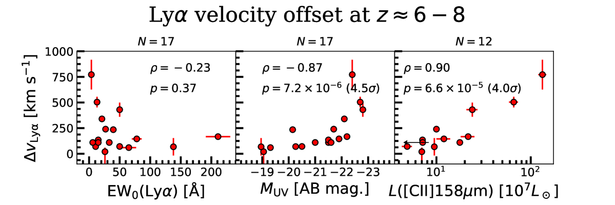
Figure 10: Compilation of Ly$\alpha$ velocity offsets at $z\approx 6-8$ from this study and the literature (Table 7). The $\Delta v_{\rm Ly\alpha}$ value is plotted against EW₀(Ly$\alpha$) (left panel), $M_{\rm UV}$ (middle panel), and the [Cii] 158  luminosity (right panel). Error bars for the literature sample are shown if available. In each panel, $N$ shows the number of individual data points. In the middle and right panels, the values of $M_{\rm UV}$ and [Cii] luminosity are corrected for magnification factors. In each panel, $\rho$ indicates the Spearman rank correlation coefficient for the relation, and $p$ denotes the probability satisfying the null hypothesis.

8.1 A consistent picture of B14-65666

B14-65666 is the first star-forming galaxy with a complete set of [Cii], [Oiii], and dust continuum emission in the reionization epoch. In conjunction with the HST F140W data (Bowler et al. 2017) and the Ly$\alpha$ line (Furusawa et al. 2016), the rich data allow us to discuss the properties of B14-65666 in detail.

In §3.2, we have inferred that B14-65666 is a merger. This is based on the fact that (i) the morphology of B14-65666 shows the two clumps in UV, [Cii], and [Oiii] whose positions are consistent with each other (Figure 1), (ii) the spectra of [Cii] and [Oiii] can be decomposed into two Gaussians kinematically separated by $\approx 200$ km s^-1 (Figures 2 and 3), and (iii) the velocity field is not smooth as expected in a rotational disk. In the same direction, Jones et al. (2017a) have concluded that a galaxy at $z=6.07$, WMH5, would be merger rather than a rotational disk based on two separated [Cii] clumps, the [Cii] velocity gradient, and the [Cii] spectral line composed of multiple Gaussian profiles.

In B14-65666, we note that the clumps A and B have UV, IR, and line luminosities that are consistent within a factor of two (Table 3.1), implying that B14-65666 would represent a major-merger at $z=7.15$. In addition, even the individual clumps have very high luminosities among $z>6$ star-forming galaxies. This suggests that B14-65666 traces a highly dense region at the early Universe. Although our current data do not show companion objects around B14-65666 (e.g., Decarli et al. 2017), future deeper ALMA data could reveal companion galaxies around B14-65666.

A merger event would enhance the star forming activity. Based on the results of our SED fitting (Table 6), we calculate the specific SFR, defined as the SFR per unit stellar mass (sSFR $\equiv$ SFR/$M_{\rm*}$). The sSFR of $260^{+119}_{-57}$ Gyr^-1 is larger than those for galaxies on the star formation main sequence at $z\approx 6-7$ (e.g., Stark et al. 2013; Speagle et al. 2014; Santini et al. 2017). This suggests that B14-65666 is indeed undergoing bursty star-formation (Rodighiero et al. 2011).

Interestingly, the high sSFR value of B14-65666 is also consistent with its relatively high luminosity-weighted dust temperature, $T_{\rm d}$ $\approx 50-60$ K, under the assumption of $\beta_{\rm d}=2.0-1.5$ (§4). Indeed, Faisst et al. (2017) have shown that objects with larger sSFR have higher $T_{\rm d}$ (see Figure 5 of Faisst et al. 2017) based on the compiled sample of local galaxies that include dwarf metal-poor galaxies, metal rich galaxies, and (ultra-)luminous infrared galaxies. Probably, a strong UV radiation field driven by intense star-formation activity in B14-65666 leads to high $T_{\rm d}$ as a result of effective dust heating (e.g., Inoue & Kamaya 2004). This hypothesis can also explain the high [Oiii]-to-[Cii] luminosity ratio in B14-65666. The strong UV radiation can efficiently ionize [Oiii] (with ionization potential of 35.1 eV) against [Cii] (ionization potential of 11.3 eV). Indeed, in the local Universe, there is a positive correlation between the [Oiii]-to-[Cii] luminosity ratio and the dust temperature (see e.g., Figure 11 in Herrera-Camus et al. 2018).

8.2 Ly$\alpha$ velocity offsets at $z\approx 6-8$ and implications for reionization: Enhanced Ly$\alpha$ visibility for bright galaxies

In this section, we discuss implications on reionization from the compiled $\Delta v_{\rm Ly\alpha}$ measurements at $z\approx 6-8$. The Ly$\alpha$ velocity offset at $z\approx 6-8$ is useful to constrain the reionization process as described below. Based on spectroscopic observations of LAEs and LBGs, previous studies have shown that the fraction of galaxies with strong Ly$\alpha$ emission increases from $z=2$ to $6$ (e.g., Cassata et al. 2015), but suddenly drops at $z>6$ (e.g., Stark et al. 2010; Pentericci et al. 2011; Ono et al. 2012; Schenker et al. 2012, 2014). This is often interpreted as a rapid increase of the neutral gas in the IGM at $z\approx 6$, significantly reducing the visibility of Ly$\alpha$. Ono et al. (2012) have revealed that the amplitude of the drop is smaller for UV bright galaxies than for UV faint galaxies. More recently, Stark et al. (2017) have demonstrated a striking LAE fraction of 100% in the sample of most luminous LBGs (Oesch et al. 2015; Zitrin et al. 2015; Roberts-Borsani et al. 2016). Stark et al. (2017) have discussed possible origins of the enhanced Ly$\alpha$ visibility of these UV luminous galaxies, one of which is that their large Ly$\alpha$ velocity offsets make Ly$\alpha$ photons less affected by the IGM attenuation when Ly$\alpha$ photons enter the IGM.

In the middle and right panels of Figure 10, we have statistically demonstrated that the $\Delta v_{\rm Ly\alpha}$ value becomes larger for galaxies with brighter UV or [Cii] luminosities at $z\approx 6-8$. This means that the Ly$\alpha$ visibility is indeed enhanced in brighter galaxies (see also Mainali et al. 2017; Mason et al. 2018b), which would give us a reasonable explanation on the high Ly$\alpha$ fraction in luminous galaxies.

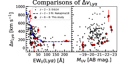
Figure 11: Comparisons of $\Delta v_{\rm Ly\alpha}$ at $z\approx 6-8$ and at $z\approx 2-3$ as a function of EW₀(Ly$\alpha$) and $M_{\rm UV}$. In each panel, the red circles show the data points at $z\approx 6-8$ whereas black small dots show data points at $z\approx 2-3$ taken from Erb et al. (2014). In the left panel, the blue dashed line indicates the average relation at $z\approx 2-3$ presented in Nakajima et al. (2018).

9 Conclusion

We have conducted high spatial resolution ALMA observations of an LBG at $z=7.15$. Our target, B14-65666, has a bright UV absolute magnitude, $M_{\rm UV}\approx$ -22.4, and has been spectroscopically identified in Ly$\alpha$ with a small rest-frame equivalent width of $\approx 4$ Å. Previous HST image has shown that the target is comprised of two spatially separated clumps in the rest-frame UV, referred to as the clump A (Northern East) and clump B (Southern West) in this study. Based on our ALMA Band 6 and Band 8 observations, we have newly detected spatially resolved [Cii] 158 , [Oiii] 88 , and dust continuum emission in the two Bands. B14-65666 is the first object with a complete set of Ly$\alpha$, [Oiii], [Cii], and dust continuum emission which offers us a unique opportunity to investigate detailed kinematical and ISM properties of high-$z$ galaxies. Our main results are as follows:

• Owing to our high spatial resolution observations, the [Cii] and [Oiii] emission can be spatially decomposed into two clumps whose positions are consistent with those of the two UV clumps revealed by HST (Figure 1). The [Cii] and [Oiii] line spectra extracted at the positions of these clumps also show that the lines are composed of two Gaussian profiles kinematically separated by $\approx 200$ km s^-1 (Figures 2 and 3). These results suggest that B14-65666 is a merger.

• The whole system, clump A, and clump B have the [Oiii] luminosity of $(34.4\pm 4.1)\times 10^{8}$, $(21.2\pm 3.2)\times 10^{8}$, and $(13.0\pm 2.1)\times 10^{8}$ $L_{\rm\odot}$, respectively, and the [Cii] luminosity of $(11.0\pm 1.4)\times 10^{8}$, $(6.0\pm 1.9)\times 10^{8}$, and $(4.9\pm 0.8)\times 10^{8}$ $L_{\rm\odot}$, respectively. The total line luminosities are the highest so far detected among $z>6$ star-forming galaxies. Even the individual clumps have very high line luminosities. The [Oiii]-to-[Cii] luminosity ratio is $3.1\pm 1.6$, $3.5\pm 0.8$, and $2.7\pm 0.6$ for the whole system, clump A, and clump B, respectively (§3; Table 3.1).

• In the whole system of B14-65666, the dust continuum flux densities at 90 and 163  are $S_{\nu,90\mu m}=470\pm 128$ and $S_{\nu,163\mu m}=130\pm 25$ $\mu$Jy, respectively. Based on the continuum ratio $S_{\nu,90\mu m}$/$S_{\nu,163\mu m}$ and assuming the emissivity index in the range of $\beta_{\rm d}=2.0-1.5$, we have estimated the dust temperature to be $T_{\rm d}$ $\approx 50-60$K. Assuming these $T_{\rm d}$ and $\beta_{\rm d}$ values, we have obtained $L_{\rm TIR}$  $\approx 1\times 10^{12}$, $3\times 10^{11}$, and $7\times 10^{11}$ $L_{\rm\odot}$ for the whole system, clump A, and clump B, respectively, by integrating the modified black-body radiation over $8-1000$ . With a typical dust mass absorption coefficient, the dust mass is estimated to be $\approx 1\times 10^{7}$ , $3\times 10^{6}$, and $6\times 10^{6}$ $M_{\rm\odot}$ for the whole system, clump A, and clump B, respectively (§4; Figure 5).

• We have investigated the IRX-$\beta$ relation at $z\approx 6.5-9.1$ based on eleven spectroscopically identified objects including five LBGs with dust continuum detections. For fair comparisons of data points, we have uniformly computed the $\beta$ and IRX values for the entire sample. We find that the five LBGs with dust detections are well characterized by the Calzetti’s dust attenuation curve (§5.1; Figure 6).

• We have created a combined sample of six galaxies with [Oiii]-to-[Cii] luminosity ratios: Our object, two literature LAEs, and three literature SMGs. We have found that the luminosity ratio becomes larger for objects with lower bolometric luminosities defined as the sum of the UV and IR luminosities. The results indicate that galaxies with lower bolometric luminosities (i.e., lower masses) have either lower metallicities or higher ionization states (§5.2; Figure 7).

• To estimate the stellar mass, SFR, and the stellar age, we have performed SED fitting for the whole system of B14-65666 taking ALMA data into account. We have obtained the total stellar mass of $\approx 7.7\times 10^{8}$$M_{\rm\odot}$ and the total SFR of $\approx 200$ $M_{\rm\odot}$ yr^-1. The specific SFR (defined as the SFR per unit stellar mass) is 260 Gyr^-1, indicating that B14-65666 is a starburst galaxy (§6; Figure 8).

• In the whole system of B14-65666, the [Cii] and [Oiii] lines have consistent redshifts of $z=7.1520\pm 0.0003$. On the other hand, Ly$\alpha$ is significantly redshifted with respect to the ALMA lines by $\Delta v_{\rm Ly\alpha}$ $=772\pm 45\pm 100$ km s^-1, which is the largest so far detected among the $z>6$ galaxy population. The very large $\Delta v_{\rm Ly\alpha}$ would be due to the presence of large amount of neutral gas or large outflow velocity (§7; Figure 9).

• Based on a compiled sample of 17 galaxies at $z\approx 6-8$ with $\Delta v_{\rm Ly\alpha}$ measurements from this study and the literature, we have found a $4.5\sigma$ ($4.0\sigma$) correlation between $\Delta v_{\rm Ly\alpha}$ and UV magnitudes ([Cii] luminosities) in the sense that $\Delta v_{\rm Ly\alpha}$ becomes larger for brighter UV magnitudes and brighter [Cii] luminosities. These results are in a good agreement with a scenario that the Ly$\alpha$ emissivity during the reionization epoch depends on the galaxy’s luminosity (§8.2; Figure 10).

Given the rich data available and spatially extended nature, B14-65666 is one of the best target for follow-up observations with ALMA and James Webb Space Telescope’s NIRSpec IFU mode to spatially resolve e.g., gas-phase metallicity, the electron density, and Balmer decrement.

Appendix A Astrometry of the HST F140W image

In this study, we compare the spatial position of B14-65666 in ALMA data with that in the HST F140W band image data (PI: R.A.A. Bowler). Several studies have reported spatial offsets between ALMA-detected objects and their HST-counterparts either due to astrometry uncertainties or physical offsets in different wavelengths (e.g., Laporte et al. 2017; González-López et al. 2017; Carniani et al. 2018b; Dunlop et al. 2017).

To better calibrate the archival F140W image, we first search for bright stars in the catalog gaiadr1.gaia${\_}$source released in the framework of the GAIA project (Gaia Collaboration et al. 2016). Similar astrometry calibrations are performed in Carniani et al. (2018b). Because of the small sky area, $\approx 2^{\prime}.3\times 2^{\prime}.0$, covered by the Bowler et al.’s archival HST data, only a single star is matched to the catalog. Thus, we instead use the catalog gaiadr1.sdssdr9${\_}$original_{_}valid from the same project. The latter catalog includes a larger number of objects while its astrometry is originally taken from the SDSS project. Using 17 objects uniformly distributed in the field-of-view, we have performed IRAF tasks ccmap and ccsetwcs to calibrate astrometry. The applied shift around B14-65666 is $\approx 0^{\prime\prime}.23$ ($\Delta_{\rm R.A.}=0^{\prime\prime}.14$ toward the West-East direction and $\Delta_{\rm Dec.}=0^{\prime\prime}.18$ toward the North-South direction) for the archival HST image. To check the accuracy of our astrometry, we make use of a serendipitous continuum detection (16$\sigma$) in Band 6 from a galaxy at $z=1.93$, COSMOS 0813412 (Schinnerer et al. 2007). Figure 12 shows that the centroids of ALMA continuum and its HST F140W counterpart are consistent with each other within $\approx 0^{\prime\prime}.15$ uncertainties, demonstrating successful astrometry calibration. We have also confirmed that the re-calibrated F140W image has astrometry consistent with that in Bowler et al. (2018) (in private communication with R. A. A. Bowler).

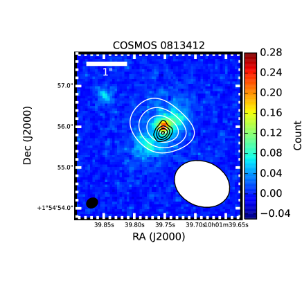
Figure 12: Black and white contours show the continuum images of a serendipitously detected object at $z=1.93$, COSMOS 0813412 (Schinnerer et al. 2007), in our ALMA Band 6 data and Bowler et al’s Band 6 data, respectively, overlaid on its counterpart in the HST F140W image with re-calibrated astrometry. Black contours are drawn at ($4$, $8$, $12$, $16$)$\times\sigma$ where $\sigma=9.5$ $\mu$Jy beam^-1 in our Band 6 data, while white contours are drawn at ($4$, $6$, $8$, $10$)$\times\sigma$ where $\sigma=27.8$ $\mu$Jy beam^-1 in Bowler et al’s Band 6 data. The ellipses at the lower left and right corner indicate the synthesized beam sizes of our and Bowler et al’s Band 6 data, respectively.

Appendix B Astrometry of Three ALMA Datasets

We present detailed analyses on astrometry of three ALMA datasets: Our ALMA Band 6 and 8 data plus Bowler et al’s Band 6 data. For this purpose, we have re-analyzed the Bowler et al’s Band 6 data using CASA ver 4.5.1. We obtain the beam size and the $1\sigma$ noise level well consistent with those presented in Bowler et al. (2018). We confirm their dust continuum detection, although the peak significance level is slightly lower, $4.6\sigma$, than the value reported in Bowler et al. (2018).

As shown in Table B, the same phase and bandpass calibrators are used in the three datasets. In addition, the same flux calibrator is used in our ALMA Band 6 and 8 data. Therefore, we firstly analyze the sky coordinates of three calibrators, J0948+0022, J1058+0133, and J0854+2006, to examine if there exists astrometry uncertainty arising from calibrators. We have confirmed that the centroids (i.e., flux peak positions) of these calibrators are consistent with each other to the order of $<0^{\prime\prime}.01$, indicating that the coordinates of the three datasets are well aligned.

Secondly, we compare the positions of COSMOS 0813412 in our and Bowler et al’s Band 6 data. Figure 12 shows the dust continuum contours of COSMOS 0813412 overlaid on the HST F140W image with re-calibrated astrometry. We obtain the centroids of (RA, Dec) = (10:01:39.753, +01.54.55.860) and (10:01:39.754, +01.54.55.920) in our and Bowler et al’s Band 6 data, respectively. This corresponds to the spatial offset of $0^{\prime\prime}.06$ toward the North-South direction. To evaluate its significance, we calculate the positional uncertainties, $\Delta p$, with the equation

$$\Delta p\ {\rm[mas]}=60\times\frac{100\ {\rm GHz}}{{\rm FREQ}}\times\frac{10\ {\rm km}}{{\rm BSL}}\times\frac{1}{{\rm SNR}},$$ (4)

where FREQ is the observing frequency in GHz, BSL is the maximum baseline length in km, and the SNR corresponds to the peak significance level. Based on FREQ $=$ 225 GHz (233 GHz), BSL $=$ 2.65 km (0.33 km), and SNR $\approx$16 (10), $\Delta p$ $=0^{\prime\prime}.01$ ($0^{\prime\prime}.08$) in our (Bowler et al’s) Band 6 data. Thus, the spatial offset of $0^{\prime\prime}.06$ is within the $1\sigma$ positional uncertainties, confirming that the two ALMA Band 6 data have consistent astrometry.

Finally, we examine the spatial positions of B14-65666 using our and Bowler et al’s Band 6 data. We do not attempt to compare the positions of B14-65666 between Band 6 and 8 data for astrometry analyses because they probe dust continuum emission at different wavelengths. Figure 13 shows the two dust continuum contours overlaid on the $4^{\prime\prime}.0\times 4^{\prime\prime}.0$ cutout image of F140W. The dust continuum centroids are obtained as (RA, Dec) = (10:01:40.683, +01.54.52.56) and (10:01:40.686, +01.54.53.00) in our and Bowler et al’s Band 6 data, respectively, corresponding to a possible spatial offset of $\Delta_{\rm tot.}=0^{\prime\prime}.44$ predominantly in the North-South direction ($\Delta_{\rm R.A.}=0^{\prime\prime}.05$, $\Delta_{\rm Dec.}=0^{\prime\prime}.44$). As in COSMOS 0813412, we calculate the positional uncertainties to be $0^{\prime\prime}.02$ ($0^{\prime\prime}.17$) in our (Bowler et al’s) Band 6 data based on the peak significance of $5.3\sigma$ ($4.6\sigma$). Therefore, the spatial offset corresponds to $2.3\sigma$ ($=0.44/(0.17+0.02)$), indicating that the offset is marginal (Table B).

Calibrators for ALMA Observations. Data phase calibrators bandpass calibrators flux calibrators (1) (2) (3) (4) This Study Band 6 (Cycle 4) J0948+0022 J1058+0133 J1058+0133, J0854+2006 Band 8 (Cycle 4) J0948+0022 J1058+0133 J1058+0133, J0854+2006 Band 8 (Cycle 5) J0948+0022, J1028-0236 J1058+0133, J1229+02023 J1058+0133, J1229+02023 Bowler et al. 2018 Band 6 (Cycle 4) J0948+0022 J1058+0133 Ganymede

Spatial Offsets of B14-65666 among the Two ALMA Band 6 Data. Data 1 Data 2 Spatial Offsets Uncertainty Significance $\Delta_{\rm tot.}$, $\Delta_{\rm R.A.}$, $\Delta_{\rm Dec.}$ Data 1, Data 2 (1) (2) (3) (4) (5) Band 6 (This Study) Band 6 (Bowler et al. 2018) $0^{\prime\prime}.44$, $0^{\prime\prime}.05$, $0^{\prime\prime}.44$ $0^{\prime\prime}.02$, $0^{\prime\prime}.17$ $2.3\sigma$ Note. (1) and (2) Two data sets to be compared; (3) Spatial offset in the units of arcsec, where $\Delta_{\rm R.A.}$ and $\Delta_{\rm Dec.}$ correspond to the offset toward the direction of R.A. and Dec., respectively, and the total offset is $\Delta_{\rm tot.}$; (4) Positional uncertainties of Data 1 and Data 2 in the units of arcsec; and (5) Statistical significance of the spatial offset.

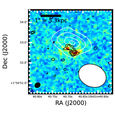
Figure 13: Black and white contours show the continuum images of B14-65666 in our ALMA Band 6 data and Bowler et al’s Band 6 data, respectively, overlaid on its counterpart in the HST F140W image with re-calibrated astrometry. Black contours are drawn at (2, 3, 4, 5)$\times\sigma$ where $\sigma=9.5$ $\mu$Jy beam^-1 in our Band 6 data, while white contours are drawn at (2, 3, 4, 4.5)$\times\sigma$ where $\sigma=27.8$ $\mu$Jy beam^-1 in Bowler et al’s Band 6 data. The ellipses at the lower left and right corner indicate the synthesized beam sizes of our and Bowler et al’s Band 6 data, respectively.

References

- Behrens et al. (2018) Behrens, C., Pallottini, A., Ferrara, A., Gallerani, S., & Vallini, L. 2018, MNRAS, 477, 552
- Binney & Tremaine (2008) Binney, J., & Tremaine, S. 2008, Galactic Dynamics: Second Edition (Princeton University Press)
- Bock et al. (1993) Bock, J. J., et al. 1993, ApJ, 410, L115
- Bouwens et al. (2009) Bouwens, R. J., et al. 2009, ApJ, 705, 936
- Bouwens et al. (2010) Bouwens, R. J., et al. 2010, ApJ, 708, L69
- Bouwens et al. (2014) Bouwens, R. J., et al. 2014, ApJ, 795, 126
- Bouwens et al. (2016) Bouwens, R. J., et al. 2016, ApJ, 833, 72
- Bowler et al. (2014) Bowler, R. A. A., et al. 2014, MNRAS, 440, 2810
- Bowler et al. (2017) Bowler, R. A. A., Dunlop, J. S., McLure, R. J., & McLeod, D. J. 2017, MNRAS, 466, 3612
- Bowler et al. (2018) Bowler, R. A. A., Bourne, N., Dunlop, J. S., McLure, R. J., & McLeod, D. J. 2018, MNRAS, 481, 1631
- Bradač et al. (2017) Bradač, M., et al. 2017, ApJ, 836, L2
- Brauher et al. (2008) Brauher, J. R., Dale, D. A., & Helou, G. 2008, ApJS, 178, 280
- Bruzual & Charlot (2003) Bruzual, G., & Charlot, S. 2003, MNRAS, 344, 1000
- Calura et al. (2017) Calura, F., et al. 2017, MNRAS, 465, 54
- Calzetti et al. (2000) Calzetti, D., Armus, L., Bohlin, R. C., Kinney, A. L., Koornneef, J., & Storchi-Bergmann, T. 2000, ApJ, 533, 682
- Capak et al. (2015) Capak, P. L., et al. 2015, Nature, 522, 455
- Carilli & Walter (2013) Carilli, C. L., & Walter, F. 2013, ARA&A, 51, 105
- Carniani et al. (2017) Carniani, S., et al. 2017, A&A, 605, A42
- Carniani et al. (2018a) Carniani, S., Maiolino, R., Smit, R., & Amorín, R. 2018a, ApJ, 854, L7
- Carniani et al. (2018b) Carniani, S., et al. 2018b, MNRAS, 478, 1170
- Cassata et al. (2015) Cassata, P., et al. 2015, A&A, 573, A24
- Chabrier (2003) Chabrier, G. 2003, ApJ, 586, L133
- Chevallard & Charlot (2016) Chevallard, J., & Charlot, S. 2016, MNRAS, 462, 1415
- Choudhury et al. (2015) Choudhury, T. R., Puchwein, E., Haehnelt, M. G., & Bolton, J. S. 2015, MNRAS, 452, 261
- Cormier et al. (2015) Cormier, D., et al. 2015, A&A, 578, A53
- Cuby et al. (2003) Cuby, J.-G., Le Fèvre, O., McCracken, H., Cuillandre, J.-C., Magnier, E., & Meneux, B. 2003, A&A, 405, L19
- da Cunha et al. (2013) da Cunha, E., et al. 2013, ApJ, 766, 13
- De Looze et al. (2014) De Looze, I., et al. 2014, A&A, 568, A62
- Decarli et al. (2017) Decarli, R., et al. 2017, Nature, 545, 457
- Dijkstra et al. (2006) Dijkstra, M., Haiman, Z., & Spaans, M. 2006, ApJ, 649, 14
- Dunlop et al. (2017) Dunlop, J. S., et al. 2017, MNRAS, 466, 861
- Dunne et al. (2000) Dunne, L., Eales, S., Edmunds, M., Ivison, R., Alexander, P., & Clements, D. L. 2000, MNRAS, 315, 115
- Ellis et al. (2013) Ellis, R. S., et al. 2013, ApJ, 763, L7
- Erb et al. (2006) Erb, D. K., Steidel, C. C., Shapley, A. E., Pettini, M., Reddy, N. A., & Adelberger, K. L. 2006, ApJ, 646, 107
- Erb et al. (2014) Erb, D. K., et al. 2014, ApJ, 795, 33
- Faisst et al. (2017) Faisst, A. L., et al. 2017, ApJ, 847, 21
- Ferland et al. (2013) Ferland, G. J., et al. 2013, RMxAA, 49, 137
- Förster Schreiber et al. (2009) Förster Schreiber, N. M., et al. 2009, ApJ, 706, 1364
- Fudamoto et al. (2017) Fudamoto, Y., et al. 2017, MNRAS, 472, 483
- Furusawa et al. (2016) Furusawa, H., et al. 2016, ApJ, 822, 46
- Gaia Collaboration et al. (2016) Gaia Collaboration et al. 2016, A&A, 595, A2
- Garel et al. (2012) Garel, T., Blaizot, J., Guiderdoni, B., Schaerer, D., Verhamme, A., & Hayes, M. 2012, MNRAS, 422, 310
- Gnerucci et al. (2011) Gnerucci, A., et al. 2011, A&A, 528, A88
- González-López et al. (2017) González-López, J., et al. 2017, A&A, 597, A41
- Gronke et al. (2015) Gronke, M., Bull, P., & Dijkstra, M. 2015, ApJ, 812, 123
- Haiman (2002) Haiman, Z. 2002, ApJ, 576, L1
- Harikane et al. (2018) Harikane, Y., et al. 2018, ApJ, 859, 84
- Hashimoto et al. (2013) Hashimoto, T., Ouchi, M., Shimasaku, K., Ono, Y., Nakajima, K., Rauch, M., Lee, J., & Okamura, S. 2013, ApJ, 765, 70
- Hashimoto et al. (2015) Hashimoto, T., et al. 2015, ApJ, 812, 157
- Hashimoto et al. (2017a) Hashimoto, T., et al. 2017a, MNRAS, 465, 1543
- Hashimoto et al. (2017b) Hashimoto, T., et al. 2017b, A&A, 608, A10
- Hashimoto et al. (2018a) Hashimoto, T., et al. 2018a, Nature, 557, 392
- Hashimoto et al. (2018b) Hashimoto, T., Inoue, A. K., Tamura, Y., Matsuo, H., Mawatari, K., & Yamaguchi, Y. 2018b, submitted to PASJ (arXiv:1811.00030)
- Herenz et al. (2016) Herenz, E. C., et al. 2016, A&A, 587, A78
- Herrera-Camus et al. (2018) Herrera-Camus, R., et al. 2018, ApJ, 861, 94
- Hildebrand (1983) Hildebrand, R. H. 1983, QJRAS, 24, 267
- Inoue & Kamaya (2004) Inoue, A. K., & Kamaya, H. 2004, MNRAS, 350, 729
- Inoue (2011a) Inoue, A. K. 2011a, MNRAS, 415, 2920
- Inoue (2011b) Inoue, A. K. 2011b, Earth, Planets, and Space, 63, 1027
- Inoue et al. (2014a) Inoue, A. K., Shimizu, I., Iwata, I., & Tanaka, M. 2014a, MNRAS, 442, 1805
- Inoue et al. (2014b) Inoue, A. K., Shimizu, I., Tamura, Y., Matsuo, H., Okamoto, T., & Yoshida, N. 2014b, ApJ, 780, L18
- Inoue et al. (2016) Inoue, A. K., et al. 2016, Science, 352, 1559
- Jiang et al. (2013) Jiang, L., et al. 2013, ApJ, 773, 153
- Jones et al. (2017a) Jones, G. C., Willott, C. J., Carilli, C. L., Ferrara, A., Wang, R., & Wagg, J. 2017a, ApJ, 845, 175
- Jones et al. (2017b) Jones, G. C., et al. 2017b, ApJ, 850, 180
- Kashino et al. (2013) Kashino, D., et al. 2013, ApJ, 777, L8
- Katz et al. (2017) Katz, H., Kimm, T., Sijacki, D., & Haehnelt, M. G. 2017, MNRAS, 468, 4831
- Knudsen et al. (2016) Knudsen, K. K., Richard, J., Kneib, J.-P., Jauzac, M., Clément, B., Drouart, G., Egami, E., & Lindroos, L. 2016, MNRAS, 462, L6
- Knudsen et al. (2017) Knudsen, K. K., Watson, D., Frayer, D., Christensen, L., Gallazzi, A., Michałowski, M. J., Richard, J., & Zavala, J. 2017, MNRAS, 466, 138
- Komatsu et al. (2011) Komatsu, E., et al. 2011, ApJS, 192, 18
- Koprowski et al. (2018) Koprowski, M. P., et al. 2018, MNRAS, 479, 4355
- Kusakabe et al. (2015) Kusakabe, H., Shimasaku, K., Nakajima, K., & Ouchi, M. 2015, ApJ, 800, L29
- Lagache et al. (2018) Lagache, G., Cousin, M., & Chatzikos, M. 2018, A&A, 609, A130
- Laporte et al. (2015) Laporte, N., et al. 2015, A&A, 575, A92
- Laporte et al. (2017) Laporte, N., et al. 2017, ApJ, 837, L21
- Laursen et al. (2013) Laursen, P., Duval, F., & Östlin, G. 2013, ApJ, 766, 124
- Madden et al. (2012) Madden, S. C., Rémy, A., Galliano, F., Galametz, M., Bendo, G., Cormier, D., Lebouteiller, V., & Hony, S. 2012, in IAU Symposium, Vol. 284, The Spectral Energy Distribution of Galaxies - SED 2011, ed. R. J. Tuffs & C. C. Popescu, 141–148
- Mainali et al. (2017) Mainali, R., Kollmeier, J. A., Stark, D. P., Simcoe, R. A., Walth, G., Newman, A. B., & Miller, D. R. 2017, ApJ, 836, L14
- Maiolino & Mannucci (2019) Maiolino, R., & Mannucci, F. 2019, A&A Rev., 27, 3
- Maiolino et al. (2015) Maiolino, R., et al. 2015, MNRAS, 452, 54
- Malhotra et al. (1997) Malhotra, S., et al. 1997, ApJ, 491, L27
- Malhotra et al. (2001) Malhotra, S., et al. 2001, ApJ, 561, 766
- Marrone et al. (2018) Marrone, D. P., et al. 2018, Nature, 553, 51
- Martin (2005) Martin, C. L. 2005, ApJ, 621, 227
- Mason et al. (2018a) Mason, C. A., Treu, T., Dijkstra, M., Mesinger, A., Trenti, M., Pentericci, L., de Barros, S., & Vanzella, E. 2018a, ApJ, 856, 2
- Mason et al. (2018b) Mason, C. A., et al. 2018b, ApJ, 857, L11
- Matsuhara et al. (1997) Matsuhara, H., Tanaka, M., Yonekura, Y., Fukui, Y., Kawada, M., & Bock, J. J. 1997, ApJ, 490, 744
- Matthee et al. (2017) Matthee, J., et al. 2017, ApJ, 851, 145
- Mawatari et al. (2016) Mawatari, K., Yamada, T., Fazio, G. G., Huang, J.-S., & Ashby, M. L. N. 2016, PASJ, 68, 46
- McMullin et al. (2007) McMullin, J. P., Waters, B., Schiebel, D., Young, W., & Golap, K. 2007, in Astronomical Society of the Pacific Conference Series, Vol. 376, Astronomical Data Analysis Software and Systems XVI, ed. R. A. Shaw, F. Hill, & D. J. Bell, 127
- Meurer et al. (1999) Meurer, G. R., Heckman, T. M., & Calzetti, D. 1999, ApJ, 521, 64
- Michałowski (2015) Michałowski, M. J. 2015, A&A, 577, A80
- Nakajima et al. (2016) Nakajima, K., Ellis, R. S., Iwata, I., Inoue, A. K., Kusakabe, H., Ouchi, M., & Robertson, B. E. 2016, ApJ, 831, L9
- Nakajima et al. (2018) Nakajima, K., Fletcher, T., Ellis, R. S., Robertson, B. E., & Iwata, I. 2018, MNRAS, 477, 2098
- Oesch et al. (2018) Oesch, P. A., Bouwens, R. J., Illingworth, G. D., Labbé, I., & Stefanon, M. 2018, ApJ, 855, 105
- Oesch et al. (2015) Oesch, P. A., et al. 2015, ApJ, 804, L30
- Oke & Gunn (1983) Oke, J. B., & Gunn, J. E. 1983, ApJ, 266, 713
- Olsen et al. (2017) Olsen, K., Greve, T. R., Narayanan, D., Thompson, R., Davé, R., Niebla Rios, L., & Stawinski, S. 2017, ApJ, 846, 105
- Ono et al. (2010) Ono, Y., Ouchi, M., Shimasaku, K., Dunlop, J., Farrah, D., McLure, R., & Okamura, S. 2010, ApJ, 724, 1524
- Ono et al. (2012) Ono, Y., et al. 2012, ApJ, 744, 83
- Ota et al. (2014) Ota, K., et al. 2014, ApJ, 792, 34
- Ouchi et al. (2013) Ouchi, M., et al. 2013, ApJ, 778, 102
- Pentericci et al. (2011) Pentericci, L., et al. 2011, ApJ, 743, 132
- Pentericci et al. (2016) Pentericci, L., et al. 2016, ApJ, 829, L11
- Popping et al. (2017) Popping, G., Somerville, R. S., & Galametz, M. 2017, MNRAS, 471, 3152
- Reddy et al. (2006) Reddy, N. A., Steidel, C. C., Fadda, D., Yan, L., Pettini, M., Shapley, A. E., Erb, D. K., & Adelberger, K. L. 2006, ApJ, 644, 792
- Rémy-Ruyer et al. (2015) Rémy-Ruyer, A., et al. 2015, A&A, 582, A121
- Richard et al. (2011) Richard, J., Kneib, J.-P., Ebeling, H., Stark, D. P., Egami, E., & Fiedler, A. K. 2011, MNRAS, 414, L31
- Rieke et al. (2009) Rieke, G. H., Alonso-Herrero, A., Weiner, B. J., Pérez-González, P. G., Blaylock, M., Donley, J. L., & Marcillac, D. 2009, ApJ, 692, 556
- Roberts-Borsani et al. (2016) Roberts-Borsani, G. W., et al. 2016, ApJ, 823, 143
- Rodighiero et al. (2011) Rodighiero, G., et al. 2011, ApJ, 739, L40
- Santini et al. (2017) Santini, P., et al. 2017, ApJ, 847, 76
- Sawicki (2012) Sawicki, M. 2012, PASP, 124, 1208
- Schaerer (2003) Schaerer, D. 2003, A&A, 397, 527
- Schaerer et al. (2015) Schaerer, D., Boone, F., Zamojski, M., Staguhn, J., Dessauges-Zavadsky, M., Finkelstein, S., & Combes, F. 2015, A&A, 574, A19
- Schenker et al. (2014) Schenker, M. A., Ellis, R. S., Konidaris, N. P., & Stark, D. P. 2014, ApJ, 795, 20
- Schenker et al. (2012) Schenker, M. A., Stark, D. P., Ellis, R. S., Robertson, B. E., Dunlop, J. S., McLure, R. J., Kneib, J.-P., & Richard, J. 2012, ApJ, 744, 179
- Schinnerer et al. (2007) Schinnerer, E., et al. 2007, ApJS, 172, 46
- Shibuya et al. (2012) Shibuya, T., Kashikawa, N., Ota, K., Iye, M., Ouchi, M., Furusawa, H., Shimasaku, K., & Hattori, T. 2012, ApJ, 752, 114
- Shibuya et al. (2014) Shibuya, T., et al. 2014, ApJ, 788, 74
- Smit et al. (2018) Smit, R., et al. 2018, Nature, 553, 178
- Sobral et al. (2015) Sobral, D., Matthee, J., Darvish, B., Schaerer, D., Mobasher, B., Röttgering, H. J. A., Santos, S., & Hemmati, S. 2015, ApJ, 808, 139
- Speagle et al. (2014) Speagle, J. S., Steinhardt, C. L., Capak, P. L., & Silverman, J. D. 2014, ApJS, 214, 15
- Stark et al. (2010) Stark, D. P., Ellis, R. S., Chiu, K., Ouchi, M., & Bunker, A. 2010, MNRAS, 408, 1628
- Stark et al. (2013) Stark, D. P., Schenker, M. A., Ellis, R., Robertson, B., McLure, R., & Dunlop, J. 2013, ApJ, 763, 129
- Stark et al. (2015a) Stark, D. P., et al. 2015a, MNRAS, 454, 1393
- Stark et al. (2015b) Stark, D. P., et al. 2015b, MNRAS, 450, 1846
- Stark et al. (2017) Stark, D. P., et al. 2017, MNRAS, 464, 469
- Steidel et al. (2010) Steidel, C. C., Erb, D. K., Shapley, A. E., Pettini, M., Reddy, N., Bogosavljević, M., Rudie, G. C., & Rakic, O. 2010, ApJ, 717, 289
- Sugahara et al. (2017) Sugahara, Y., Ouchi, M., Lin, L., Martin, C. L., Ono, Y., Harikane, Y., Shibuya, T., & Yan, R. 2017, ApJ, 850, 51
- Takeuchi et al. (2012) Takeuchi, T. T., Yuan, F.-T., Ikeyama, A., Murata, K. L., & Inoue, A. K. 2012, ApJ, 755, 144
- Tamura et al. (2018) Tamura, Y., et al. 2019, ApJ, 874, 27
- Trainor et al. (2015) Trainor, R. F., Steidel, C. C., Strom, A. L., & Rudie, G. C. 2015, ApJ, 809, 89
- Vallini et al. (2017) Vallini, L., Ferrara, A., Pallottini, A., & Gallerani, S. 2017, MNRAS, 467, 1300
- Vallini et al. (2015) Vallini, L., Gallerani, S., Ferrara, A., Pallottini, A., & Yue, B. 2015, ApJ, 813, 36
- Vanzella et al. (2011) Vanzella, E., et al. 2011, ApJ, 730, L35
- Verhamme et al. (2015) Verhamme, A., Orlitová, I., Schaerer, D., & Hayes, M. 2015, A&A, 578, A7
- Verhamme et al. (2006) Verhamme, A., Schaerer, D., & Maselli, A. 2006, A&A, 460, 397
- Verhamme et al. (2018) Verhamme, A., et al. 2018, MNRAS, 478, L60
- Walter et al. (2018) Walter, F., et al. 2018, ApJ, 869, L22
- Watson et al. (2015) Watson, D., Christensen, L., Knudsen, K. K., Richard, J., Gallazzi, A., & Michałowski, M. J. 2015, Nature, 519, 327
- Weiner et al. (2009) Weiner, B. J., et al. 2009, ApJ, 692, 187
- Willott et al. (2015) Willott, C. J., Carilli, C. L., Wagg, J., & Wang, R. 2015, ApJ, 807, 180
- Willott et al. (2013) Willott, C. J., Omont, A., & Bergeron, J. 2013, ApJ, 770, 13
- Zheng et al. (2014) Zheng, W., et al. 2014, ApJ, 795, 93
- Zheng et al. (2017) Zheng, W., et al. 2017, ApJ, 836, 210
- Zheng & Wallace (2014) Zheng, Z., & Wallace, J. 2014, ApJ, 794, 116
- Zitrin et al. (2015) Zitrin, A., et al. 2015, ApJ, 810, L12