Variability Timescale and Spectral Index of Sgr A* in the Near Infrared:
Approximate Bayesian Computation Analysis of the
Variability of the Closest Supermassive Black Hole

Abstract

Sagittarius A* (Sgr A*) is the variable radio, near-infrared (NIR), and X-ray source associated with accretion onto the Galactic center black hole. We present an analysis of the most comprehensive NIR variability dataset of Sgr A* to date: eight 24 hr epochs of continuous monitoring of Sgr A* at 4.5 µm with the IRAC instrument on the Spitzer Space Telescope, 93 epochs of 2.18 µm data from Naos Conica at the Very Large Telescope, and 30 epochs of 2.12 µm data from the NIRC2 camera at the Keck Observatory, in total 94,929 measurements. A new approximate Bayesian computation method for fitting the first-order structure function extracts information beyond current fast Fourier transformation (FFT) methods of power spectral density estimation . With a combined fit of the data of all three observatories, the characteristic coherence timescale of Sgr A* is $\tau_{b}=243^{+82}_{-57}$ minutes ($90\%$ credible interval). The PSD has no detectable features on timescales down to 8.5 minutes ($95\%$ credible level), which is the ISCO orbital frequency for a dimensionless spin parameter $a=0.92$. One light curve measured simultaneously at 2.12 and 4.5 µm during a low flux-density phase gave a spectral index $\alpha_{s}=1.6\pm 0.1$ ($F_{\nu}\propto\nu^{-\alpha_{s}}$). This value implies that the Sgr A*  color becomes bluer during higher flux-density phases. The probability densities of flux densities of the combined datasets are best fit by log-normal distributions. Based on these distributions, the Sgr A* spectral energy distribution is consistent with synchrotron radiation from a non-thermal electron population from below 20 GHz through the NIR.

1 Introduction

The broadband radiation source Sgr A* is located at the heart of the so-called S-star cluster (Sabha et al., 2012) at the center of the Milky Way. Sgr A*’s position is coincident with the dynamical center of the S-stars and therefore coincident with the dynamically derived location (to within $\sim$2 mas) of the central supermassive black hole (SMBH) of our Galaxy (e.g., Yelda et al. 2010). That makes Sgr A*  more than 100 times closer than any other supermassive black hole (SMBH), and it can therefore be studied in far greater detail.

Sgr A* is visible as a compact, moderately variable radio source having flux densities between 0.5 and 4 Jy in the range 0.1 to 360 GHz (Balick & Brown 1974; Falcke et al. 1998; Falcke & Markoff 2000; Zhao et al. 2001; Herrnstein et al. 2004; Miyazaki et al. 2004; Mauerhan et al. 2005; Yusef-Zadeh et al. 2006a; Marrone et al. 2008; Yusef-Zadeh et al. 2009; Li et al. 2009; Kunneriath et al. 2010; García-Marín et al. 2011; Bower et al. 2015; Rauch et al. 2016; Capellupo et al. 2017). Sgr A* has much dimmer NIR and X-ray counterparts that are variable by up to 30 times the mean flux density in the NIR and up to a factor 500 in the X-rays (Baganoff et al. 2001; Hornstein et al. 2002; Genzel et al. 2003; Ghez et al. 2004; Eisenhauer et al. 2005; Hornstein et al. 2007; Meyer et al. 2008; Porquet et al. 2008; Do et al. 2009; Dodds-Eden et al. 2009; Sabha et al. 2010; Dodds-Eden et al. 2011; Witzel et al. 2012; Neilsen et al. 2013, 2015; Ponti et al. 2017; Zhang et al. 2017). The X-ray energy output can become comparable to the submm level during the brightest flares. This strong, rapid variability may be associated with accretion processes close to the supermassive black hole’s event horizon. The connection of the variability to regions close to the event horizon is based on: (1) the observed timescales of the variability, with common changes of a factor $\gtrsim$10 within $\sim$10 minutes in the NIR (Genzel et al. 2003; Ghez et al. 2004); (2) the spectral index $\alpha_{s}\approx 0.6$ (Ghez et al. 2005b; Hornstein et al. 2007; Bremer et al. 2011; Witzel et al. 2014); (3) linear polarization in the NIR and submm (Eckart et al. 2006a; Marrone et al. 2006; Meyer et al. 2006b; Trippe et al. 2007; Marrone et al. 2007; Eckart et al. 2008a; Yusef-Zadeh et al. 2007; Nishiyama et al. 2009; Witzel et al. 2011; Shahzamanian et al. 2015); and (4) temporal correlations between the submm, NIR, and X-ray regimes. All of these observational results point to a population of relativistic electrons in a region that is smaller than $\sim$10 light minutes (the distance associated with the light crossing time, $<$15 Schwarzschild radii) emitting synchrotron radiation at NIR wavelengths. The variable submm and X-ray radiation may be synchrotron emission or may be linked by radiative transfer processes such as adiabatic expansion and inverse Compton or synchrotron self-Compton scattering, respectively (Baganoff et al. 2001; Eckart et al. 2004, 2006b; Gillessen et al. 2006; Yusef-Zadeh et al. 2006a, b; Eckart et al. 2008b, a; Marrone et al. 2008; Yusef-Zadeh et al. 2008; Dodds-Eden et al. 2009; Yusef-Zadeh et al. 2009; Trap et al. 2011; Eckart et al. 2012; Yusef-Zadeh et al. 2012; Haubois et al. 2012; Mossoux et al. 2016; Rauch et al. 2016; Dibi et al. 2016; Ponti et al. 2017).

In order to shed light on the physical and radiative mechanisms at work and on the interrelation between wavelengths, many studies have attempted to find and categorize recurring patterns and regularities in the behavior of Sgr A*, both statistically for individual wavelength regimes as well as in the form of correlations between bands (Meyer et al. 2007, 2006a, 2006b; Gillessen et al. 2006; Hornstein et al. 2007; Do et al. 2009; Meyer et al. 2009; Zamaninasab et al. 2010; Dodds-Eden et al. 2011; Witzel et al. 2012; Neilsen et al. 2013; Meyer et al. 2014; Hora et al. 2014; Dexter et al. 2014; Neilsen et al. 2015; Subroweit et al. 2017). In recent years, the preponderance of studies has arrived at the following set of phenomenological but statistically rigorous results:

• Sgr A* is a continuously variable NIR source that emits above the 2.12 µm detection level (0.05 mJy observed or 0.5 mJy dereddened, 3$\sigma$ above the noise level of the NIRC2 camera at the Keck II telescope) $\sim$90% of the time (Witzel et al. 2012; Meyer et al. 2014). Its probability density function (PDF) of flux densities at 2.18 µm is highly skewed (Dodds-Eden et al. 2011) and can be described by a power law with a slope $\beta_{\rm{IR}}\approx 4$ (Witzel et al. 2012). The first three moments of the PDF are well defined with mean $\approx$5.8 mJy dereddened ($\approx$0.6 mJy observed), variance $\approx$9.4 mJy² dereddened, and skewness $\approx$52.3 mJy³ dereddened. The brightest observed NIR peak reached $\sim$30 mJy (dereddened, Dodds-Eden et al. 2009). Peaks with $F(2.18~{}\micron)>10$ mJy (dereddened) occur about four times a day (Do et al. 2009; Meyer et al. 2009, 2014; Hora et al. 2014).

• The X-ray emission comes from a steady, extended ($\sim$1″) source plus outbursts from an unresolved source. Outburst flux densities can be several hundred times the level of the quiescent state. Outbursts (frequently called ”flares” in the literature) have the character of distinct events and occur about once per day. The unresolved source is detectable only during its outbursts. At other times, fluctuations are sufficiently described by the Poisson distribution expected for the steady source (Neilsen et al. 2015). The flux-density PDF, as for the NIR, is well described by a power-law distribution but with $\beta_{X}\approx 2$. X-ray flares seem always to be accompanied by NIR peaks (Morris et al. 2012 and references therein). However, the reverse is not true, and only about one in four $F(2.18~{}\micron)>10$ mJy (dereddened) NIR peaks has an X-ray counterpart (Baganoff et al. 2001; Eckart et al. 2004; Marrone et al. 2008; Porquet et al. 2008; Do et al. 2009; Neilsen et al. 2013, 2015). There is no obvious relationship between X-ray and NIR flux-density levels.

• The spectral energy distribution of Sgr A* peaks in the submm (Zylka et al. 1992, 1995; Falcke et al. 1998; Melia & Falcke 2001), where it is visible as a synchrotron source powered by the dominant thermal electron population (Yuan et al. 2003). An analysis by Dexter et al. (2014) of $\sim$10 years of 1.3, 0.87, and 0.43 mm observations with CARMA and SMA shows a steady flux-density level of $\sim$3 Jy with Gaussian fluctuations about that mean. Submm flux-density enhancements rising $\sim 1$ Jy above the mean occur approximately 1.2 times per day (Marrone et al. 2008). A time-series analysis of submm light curves gave a mean reversion time scale of $\sim$8 hr (Dexter et al. 2014).

The patterns of correlation between wavelengths are still unclear. Several authors have suggested that the submm peaks often follow bright NIR peaks by 1–3 hr (Marrone et al. 2008; Eckart et al. 2006b; Yusef-Zadeh et al. 2006a; Eckart et al. 2008b; Yusef-Zadeh et al. 2009; Eckart et al. 2009; Yusef-Zadeh et al. 2011; Eckart et al. 2012), but most observations remain inconclusive in this regard because of the lack of simultaneous multi-wavelength data of sufficient length and overlap. Indeed, there are counterexamples. Recent observations obtained with the Spitzer Space Telescope, the Chandra X-ray Observatory, the SMA, and the W. M. Keck Observatory suggest that the phenomenology of these correlations is not simple (Fazio et al., 2018). In particular, SMA and Spitzer observed the first example of an effectively synchronous sequence of variations in the submm and NIR. Another example obtained with SMA, Chandra, and Keck showed an even more surprising sequence in which a submm peak precedes an X-ray flare, which in turn was followed by a NIR peak. Albeit not conclusive due to the limitations of ground-based observations, such a sequence of peaks contradicts the canonical phenomenology of simultaneous X-ray and NIR followed by delayed submm variations.

There are many previous studies of the statistical properties of Sgr A*’s variability. Initially, these studies focused on putative quasi-periodicity (QPO) at time scales between 10 and 20 minutes and its relation to the innermost stable orbit of the $4\times 10^{6}~{}\rm{M}_{\odot}$ SMBH (Genzel et al. 2003; Meyer et al. 2006b, a, 2007; Trippe et al. 2007; Zamaninasab et al. 2010; Karssen et al. 2017). Do et al. (2009) found no evidence for such a QPO based on available data at the time. Consequently, the scope of the statistical analysis was broadened with a determination of the red-noise correlation timescale ($128^{+329}_{−77}$ minutes) in the NIR (Meyer et al. 2009) that allowed for a comparison of Sgr A* with black holes of different mass regimes. This comparison revealed that the mass and characteristic timescale of Sgr A* are consistent with a linear mass–timescale relation without a luminosity correction term as proposed by, for example, McHardy et al. (2006), who discussed characteristic timescales of AGN and black hole X-ray binaries (BHXRB). In this context, Meyer et al. (2009) pointed out the value of Sgr A* because it is the SMBH with the most precise mass determination so far: ${M}_{\rm{bh}}=(4.02\pm 0.16\pm 0.04)\times 10^{6}$ M_☉ (Boehle et al., 2016), where the error bar terms give the statistical and systematic uncertainties, respectively.

Another line of inquiry has considered the possibility of a dichotomy of the NIR variability into statistically different processes (or ‘states’) with either different flux-density PDFs or different timing behavior or both. These inquiries have been motivated by some NIR flares having X-ray counterparts while others do not (Dodds-Eden et al. 2011). The statistics of the variations have been shown to be consistent with a single variability state without evidence for multiple superimposed or interleaved variability processes (Witzel et al. 2012; Meyer et al. 2014).

A variety of NIR spectral index values have been reported. While some authors found a strong dependence of the spectral index on the flux-density level, high-cadence and high-signal-to-noise studies showed only minor intrinsic fluctuations around an $H$- (1.65 µm) to $L$-band (3.8 µm) spectral index $\alpha_{s}=0.6$ (Eisenhauer et al. 2005; Ghez et al. 2005b; Gillessen et al. 2006; Krabbe et al. 2006; Hornstein et al. 2007; Bremer et al. 2011; Witzel et al. 2014).

Sgr A* is linearly polarized in the NIR. Shahzamanian et al. (2015) statistically analyzed time series and found typical polarization of $(20\pm 10)\%$ and a preferred position angle of $(13\pm 15)\arcdeg$.

In summary, the NIR variability is well characterized as a red-noise process – that is, it has a power spectral density (PSD) that is a power law with a slope $\gamma_{1}\approx 2$ for timescales in the range $\sim$20 to $\sim$150 minutes. The process is a damped random walk – that is, it has a correlation (or characteristic) timescale. For timescales longer than the correlation timescale ($128^{+329}_{−77}$ minutes at the 90% credible level—Meyer et al. 2009), the process is uncorrelated white noise, and the PSD becomes flat for the corresponding lowest frequencies (see Appendix B.1). Based on the available datasets, no evidence for periodicity, quasi-periodicity, or changes in its statistical behavior (e.g., a two-state variability model) could be found. In fact, the existing knowledge of the NIR variability of Sgr A* can be described statistically by as few as five parameters: the PSD slope and break timescale, the slope and normalization of the power-law flux-density PDF, and the NIR spectral index. Two more parameters are needed to describe the linear polarization: the fixed polarization fraction and position angle. Considering the large amplitudes of flux-density fluctuations, such constancy of statistical and physical parameters over the period of existing data is surprising.

Specific scenarios for producing NIR variability have invoked magnetic reconnection events, disk instabilities, ejection and expansion of plasma blobs, unsteady jet emission, or accretion of magnetic fields (Sharma et al. 2007; Yuan & Bu 2010; Dodds-Eden et al. 2010; Eckart et al. 2012). However, these theoretical efforts to model the turbulent accretion flow and the variability caused by the accretion cannot fully explain all observations to date. In particular, the peak NIR flux densities are higher than predicted by radiative transfer models of three-dimensional general relativistic magnetohydrodynamic (GRMHD) simulations with a thermal electron distribution function that matches millimeter flux densities. The observed NIR variability may therefore be due to the acceleration of electrons out of the dominant thermal component of the distribution function into a non-thermal tail (e.g., Dodds-Eden et al. 2010).

GRMHD models with a thermal electron distribution, while producing only relatively weak variability (Dolence et al. 2012), have an interesting feature in their power spectrum near $f_{\rm{ISCO}}$, the orbital frequency of the innermost stable circular orbit (ISCO). In particular, these models show an approximately $f^{-2}$ power spectrum at $f<f_{\rm{ISCO}}$, a bump in power close to $f_{\rm{ISCO}}$, and a break in the spectrum to approximately $f^{-4}$ at $f>f_{\rm{ISCO}}$. This is consistent with the notion that variability in the disk at frequencies above the orbital frequency is associated with disk turbulence, which is known from simulations to have a steeply declining spatial power spectrum (e.g., Guan et al. 2009). This would naturally give rise to a steeply declining temporal power spectrum as well. With Spitzer (Hora et al. 2014), in combination with ground-based 8–10 m telescopes, the predicted PSD short-timescale structure is testable.

This work presents the first analysis of the NIR PSD of Sgr A* that includes continuous datasets for all relevant timescales from 24 hr down to the sub-minute level. We use an unprecedented dataset from three different observatories: the W. M. Keck Observatory, the European Southern Observatory Very Large Telescope (ESO/VLT), and the Spitzer Space Telescope. The observatories contribute complementary information about the PSD: the Keck data have the best signal-to-noise and can detect Sgr A* variations at timescales below 1 minute. A limitation is that most of the Keck datasets have a duration of $\leq$2 hr. The VLT data cover timescales between 4 minutes and 6 hr, and the Spitzer data timescales from $\sim$7 minutes to 24 hr, much longer than the previously derived correlation timescale. Together, these data enable the most precise estimate possible today of the correlation timescale and a test for PSD features at timescales below 50 minutes.

To exploit the combined data sets, we have developed an entirely new algorithm. It uses the first-order structure function as the central tool for analyzing the timing of Sgr A* and a customized population Monte Carlo approximate Bayesian computation (PMC-ABC) sampler to derive parameter values. The goals of this paper are to

• provide this extensive dataset to the community with a full statistical characterization;

• introduce the new PMC-ABC algorithm that will have wide application to variable sources;

• determine the PSD of the variability process of Sgr A*, including a new determination of the correlation timescale;

• determine the Sgr A* flux-density PDF in both $K$- and $M$-band (4.5 µm);

• characterize the Sgr A* spectral index between these two bands; and

• characterize the instrumental performance of this kind of space-based variability study in comparison to ground-based AO telescopes.

Section 2 describes the observations and datasets used in this work. Section 3 and Appendix B present the newly developed algorithm for analyzing non-deterministic stationary linear time series and the results of our analysis of the Sgr A* light curves. Sections 4 and 5 discuss the results and present our conclusions.

Different authors (e.g., Genzel et al. 2003; Do et al. 2009; Dodds-Eden et al. 2011) have used different values for interstellar extinction to Sgr A*, making it difficult to compare studies. To avoid ambiguity and simplify comparisons, data are given here without correction for interstellar extinction, contrary to prior practice (e.g., Witzel et al. 2012). Where extinction is needed, for example to compare with models or discuss an intrinsic spectral index, we adopt a 2.12 and 2.18 $\mu$m extinction $A_{K}=2.46\pm 0.10$ mag (Schödel et al. 2010, 2011) and a 4.5 $\mu$m extinction value of $A_{M}=1.00\pm 0.14$ mag. To place our $K$-band flux densities on the same scale as Dodds-Eden et al. (2011) or Witzel et al. (2012), multiply by 9.64 ($A_{K}=2.46$). To compare with Genzel et al. (2003) or Eckart et al. (2006b), multiply by 13.18 ($A_{K}=2.8$). To compare with Do et al. (2009), multiply by 20.89 ($A_{K}=3.3$), and to compare with Hornstein et al. (2007), multiply by 19.23 ($A_{K}=3.2$).

2 Observations and Data Reduction

2.1 Spitzer/IRAC observations

All observations in this Spitzer Space Telescope program (Program IDs 10060, 12034, and 13027) used IRAC subarray mode, which reads a 32$\times$32-pixel region of the IRAC 4.5 µm detector array 10 times per second. Each subarray data collection event obtains 64 consecutive images (a “frame set”) of these pixels, and there is typically 2 s idle time between images. The subarray pixel area starts at pixel (9,9) of the full 256$\times$256-pixel array, and the angular scale is 1$\farcs$21 per pixel.

Each of eight Spitzer observing epochs used the same basic observing procedure. This comprised an initial peakup from a reference star to place Sgr A* at the center of pixel (16,16), making a small map, during which time the telescope temperature settled down, a second peakup, a staring mode observation lasting $\sim$12 hr, a third peakup, and a second stare. The staring observations in 2013 and 2014 used custom Instrument Engineering Requests (IERs) to obtain two 11.6 hr monitoring periods at each epoch. The 2016 observations used standard Astronomical Observation Requests (AORs) to do the same, but with $2\times 12$ hr of monitoring. The 2017 observations used new IERs to decrease the effective data rate by truncating the lowest four bits of each 0.1 s pixel value. Because of the high source brightness in the Galactic center, these bits contain random noise and therefore do not compress. Removing them reduced the data volume to 65% of what it would have been without truncating. Prior to making the 2017 observations, we used our earlier Sgr A* measurements to verify that truncating these bits would increase the noise by only $\sim$1.3%, which does not affect our ability to measure flux density fluctuations at expected levels. Further details of the observations are given by Hora et al. (2014), and all AORKEYs are in Table 1.

Table 1: IRAC Observation Log

	AOR Start	Frame
AORKEY	Time (UTC)	Sets	Type
50123264	2013-12-10 03:48:56	92	Map
50123520	2013-12-10 04:20:24	5000	Stare part 1
50123776	2013-12-10 16:04:21	5000	Stare part 2
51040768	2014-06-02 22:32:00	126	Map
51041024	2014-06-02 22:59:37	5000	Stare part 1
51041280	2014-06-03 10:43:22	5000	Stare part 2
51087616	2014-06-17 18:29:35	126	Map
51087872	2014-06-17 18:57:17	5000	Stare part 1
51088128	2014-06-18 06:41:01	5000	Stare part 2
51344128	2014-07-04 13:21:59	126	Map
51344384	2014-07-04 13:49:41	4999	Stare part 1
51344640	2014-07-05 01:33:25	5000	Stare part 2
58115840	2016-07-12 18:04:23	156	Map
58116352	2016-07-12 18:37:45	5142	Stare part 1
58116608	2016-07-13 06:41:14	5142	Stare part 2
58116096	2016-07-18 11:44:02	156	Map
58116864	2016-07-18 12:17:25	5142	Stare part 1
58117120	2016-07-19 00:20:54	5142	Stare part 2
60651008	2017-07-15 22:28:54	156	Map
63303680	2017-07-15 23:02:17	5142	Stare part 1
63303936	2017-07-16 11:05:46	5142	Stare part 2
60651264	2017-07-25 22:39:33	156	Map
63304192	2017-07-25 23:12:57	5142	Stare part 1
63304448	2017-07-26 11:16:26	5141	Stare part 2

Table 2: IRAC Flux Correction Coefficients

Coefficient	2013	2014	2014	2014	2016	2016	2017	2017
Name	Dec 10	June 2	June 17	July 4	July 12	July 18	July 15	July 25
$a$	7537.1	5358.9	3693.5	6684.6	$-$877.31	4748.0	4555.274	6938.5
$b$	$-$17216	$-$1336.0	3173.4	$-$9461.1	$-$22340	27.372	$-$4669.305	15146.3
$c$	3730.1	$-$2696.0	1679.9	$-$12401	$-$12402	$-$2525.2	$-$4963.178	13822.1
$d$	-$11716$	-$6104.9$	9248.1	9199.4	$-$6054.6	$-$9.3296	$-$102.5009	14876.4
$e$	3396.5	-$1074.1$	7629.8	5026.4	9508.4	-$5798.4$	$-$3444.561	2254.8
$f$	-$3025.0$	-$760.80$	16120	15750	10070	391.47	5618.444	23499.7
$g_{1}$	0.0054	0.3611	$-$0.0049	0.1732	0.3128	$-$0.0004	0.05112	0.05934
$g_{2}$	$-$0.0451	$-0.2359$	0.1518	$-0.2194$	0.3267	0.4427	0.03646	$-$0.1593
$g_{3}$	$-$0.0007	0.1785	0.0344	$-$0.2423	0.1124	$-0.1267$	0.06231	0.1074
$g_{4}$	0.04063	$-$0.2422	0.1685	0.1462	0.0672	$-0.2089$	0.05674	$-$0.02738
$h_{1}$	0.2897	$-$0.7424	$-$0.2675	$-$0.5568	1.3735	$-0.2927$	0.4828	0.1101
$h_{2}$	1.338	0.5666	$-$0.4242	0.9940	1.1245	$-0.7833$	0.8234	0.8551
$h_{3}$	0.1075	$-0.6004$	0.4291	0.9720	1.0763	1.5937	0.1941	$-$1.3753
$h_{4}$	0.4762	1.1260	$-0.6078$	$-0.2426$	0.9778	1.1396	0.6042	$-$0.9479
$k_{1}$	0.0679	$-$0.7136	0.6420	$-0.5358$	0.0466	$-$1.0620	$-$0.0834	$-$0.0098
$k_{2}$	0.1133	0.8440	$-0.7912$	0.9836	$-$0.1290	$-$1.0258	$-$1.3781	$-$1.0708
$k_{3}$	$-$0.3432	$-$0.2633	$-$0.1390	1.6669	$-$0.0074	$-$0.3891	0.1371	0.3808
$k_{4}$	$-$0.0905	0.5196	$-$0.3543	$-$0.3662	$-$0.0981	0.9668	1.0882	0.6798

The data reduction used an improved version of the technique described by Hora et al. (2014). The first image of every frame set was removed because of calibration difficulties, and the remaining 63 frames were averaged. The major remaining problem is that telescope pointing jitter introduces fluctuations into the flux measured by pixel (16,16). Those can be largely removed by fitting the measured flux as a function of the $(X,Y)$ coordinates of Sgr A* in each frame set with $(X,Y)$ being determined by cross-correlating each frame set with a standard one having Sgr A* centered on pixel (16,16). However, this basic scheme does not work as well for the epoch 2–8 observations (2014 June–July) as it did for the first epoch (2013 December). This may be due to the observations being performed at a different rotation angle on the array than the first epoch. The new angle did not allow the same simple correction to yield similar quality as in the first epoch, probably due to the inherent structure of the source and the details of how it falls on the pixel array. For some reason, the $(X,Y)$ coordinates do not capture all of the apparent background variability. Several methods were tried to improve the fit. We found that the dependence of the pixel output $F(X_{i},Y_{i})$ on the $X,Y$ position on the array for the object and reference pixels could be well-modeled by using the second-degree polynomial

$$\begin{split}F(X_{i},Y_{i})=a+bX_{i}+cY_{i}+dX_{i}Y_{i}+eX_{i}^{2}+fY_{i}^{2}+\\ \sum_{n=1}^{4}{P_{i,n}(g_{n}+h_{n}X_{i}+k_{n}Y_{i})}\quad,\end{split}$$ (1)

where $a,b,c,d,e,f,g_{n},h_{n}$, and $k_{n}$ are constant coefficients to be derived; $i$ is the sample number in the time sequence; $X_{i}$ and $Y_{i}$ represent the position of Sgr A* on the array for sample $i$ in units of pixels (relative to the center of pixel (16,16)); and $P_{i,n}$ are the data values of the four pixels that are direct neighbors to the pixel output being analyzed. For example, for the analysis of pixel (16, 16), these neighbor pixels were (15,16), (17,16), (16,15), and (16,17). The values of the coefficients were determined by least-squares fitting, minimizing the residuals between $F(X_{i},Y_{i})$ and the pixel (16,16) values in the monitoring data. The fit was done iteratively, removing frame sets in which Sgr A* showed detectable flux. That typically left about 7000 frame sets to fit out of an initial $>$10,000 available in each epoch. Coefficients derived for each epoch are given in Table 2.

As a test of our method, we also extracted and modeled the output of a reference pixel in the same way as for pixel (16,16). The reference pixel was at an image location with a significant gradient and not on a local maximum, similar to pixel (16,16) but far enough away from it that the pixel will not see the variability from Sgr A*. For the 2013 December epoch, we used pixel (18,19) as a reference, as did Hora et al. (2014). Because of the different rotation angle in all subsequent epochs, we used pixel (14,14).

One limitation of the reduction technique is that it cannot provide an absolute zero point for the Sgr A* flux density. Instead, $F=0$ corresponds to the average flux density in the frame sets used to derive the coefficients. The actual flux density corresponding to $F=0$ is a parameter derived from subsequent fitting of the time-series data.

The eight light curves are plotted in Figure 1, and the time series data are given in Table 3. The new reduction of the 2013 epoch is very similar to the original result of Hora et al., but the artifacts in the reference pixel are smaller compared to the original reduction. The peaks of emission from Sgr A* in the 2013 epoch are in the same locations and very similar in amplitude and structure.

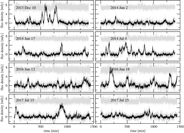
Figure 1: Excess 4.5 µm flux density for Sgr A* and for the reference pixel for each of the eight Spitzer epochs. Flux densities are in mJy with no correction for interstellar extinction. The flux density zero point cannot be determined by the data reduction method. In each panel, the gray lines show the flux density for each 6.4-s frame set, and the black lines show the data binned in one minute intervals. The lower lines show the Sgr A* flux densities, and the upper lines are for a reference pixel with $7$ mJy added to the flux density. The 2013 December epoch uses pixel (18,19) as the reference, and all other epochs use pixel (14,14). The values plotted are the difference between the observed value of the pixel in the 6.4-s frame set and the predicted value based on Eq. 1 and the measured $(X,Y)$ offset of each frame set. Flux density values have been corrected to total flux density for a point source by the position-dependent ratio of total flux density to central-pixel signal. The horizontal axis shows the time in minutes relative to the start time (given in Table 1) of the first monitoring 6.4-s frame set for that epoch.

Table 3: Sgr A* Light Curve Data

Observation	Sgr A*	Reference
Date	Flux Density	Flux Density
(HMJD)	(Jy)	(Jy)
Spitzer/IRAC
…
57581.7781761	0.001056	0.000016
57581.7782728	0.001576	-0.000329
57581.7783700	0.001055	0.000182
57581.7784676	-0.000623	0.000908
57581.7785647	0.001590	-0.000180
57581.7786621	-0.000930	-0.001045
57581.7787590	0.000980	-0.000776
57581.7788565	-0.000085	0.000744
57581.7789539	0.000819	-0.000939
57581.7790510	-0.000407	0.000747
…
VLT/NaCo
52803.1129224	0.0001745
52803.1133356	0.0001585
52803.1137607	0.0000846
52803.1141797	0.0001671
52803.1145983	0.0001632
52803.1150173	0.0001849
52803.1154358	0.0001362
52803.1158572	0.0001725
52803.1162806	0.0001702
52803.1166930	0.0001488
…
Keck/NIRC2
53212.3510956	0.0004091
53212.3529755	0.0005316
53212.3532755	0.0004738
53212.3539055	0.0006439
53212.3550154	0.0005638
53212.3555354	0.0003294
53212.3796940	0.0000225
53551.3979607	0.0000009
53581.3320382	0.0001165
53581.3369779	0.0001175
…

All eight Spitzer epochs showed flux-density variations intrinsic to Sgr A* in the range of $\sim$0–8.5 mJy (not dereddened; see Figure 2). The first and the sixth epochs (2013 December 10, 2016 June 18) showed the highest peaks and the longest-duration excursions from zero. In contrast, the epoch of 2014 June 2 showed only minor excursions during the $>$23 hr of observations. The noise characteristics of the Spitzer data can be estimated using the flux-density PDF of the reference pixels (shown in Figure 2), which has a standard deviation $\sigma_{\rm IRAC}=0.66$ mJy for one 6.4 s frame set.

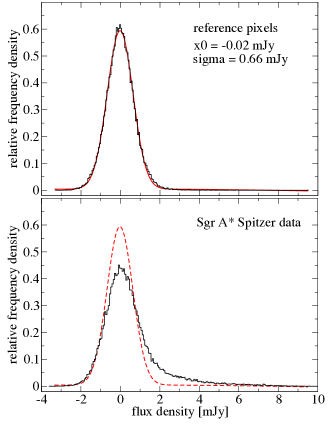
Figure 2: Normalized flux density distributions for the combined IRAC data. Black curves show the observed distributions: the reference pixel in the upper panel and Sgr A* in the lower panel. The red dashed curve in both panels shows a Gaussian distribution centered at $x_{0}=-0.02$ mJy and with a standard deviation $\sigma=0.66$ mJy.

2.2 Ground-based observations with VLT and Keck

The VLT data (previously reported by Witzel et al. 2012) were taken with the adaptive optics camera Naos Conica (NaCo; Lenzen et al. 2003) in $K_{s}$-band (2.18 µm). The NaCo images have 68 mas resolution and integration times of 30–40 s. Data were taken between 2003-06-13 and 2010-06-16. The complete data set, after rejecting images with unstable zero points, contains 10,639 images. The average cadence of the observations is one image per 1.2 minutes, the cadence being limited by deliberate telescope offsets (“dithering”) between frames. Witzel et al. (2012) provided an observing log, and described the data reduction and calibration.

The Keck data were obtained with the NIRC2 camera (PI Keith Matthews) in the $K’$-band (2.12 µm). Images have 53 mas resolution and a fixed integration time of 28 s. The data set contains 3157 images between 2004-07-16 and 2013-07-19. The average cadence was one image per 1.1 minutes, again limited by dithering. Table 4 lists the Keck epochs analyzed here.

Table 4: Keck/NIRC2 Observation Log

Date	Start time	Stop time	Duration	Number
(UT)	(UT)	(UT)	(minutes)	of frames
2004-07-26	08:18:50	09:00:01	41.18	7
2005-07-30	07:51:43	08:47:24	55.68	4
2006-05-03	11:03:03	13:14:12	131.14	26
2006-06-20	08:59:22	11:04:45	125.38	90
2006-06-21	08:52:27	11:36:53	164.43	163
2006-07-17	06:47:50	09:54:03	186.22	63
2007-05-17	11:08:23	13:52:39	164.26	81
2007-08-10	06:54:19	08:21:05	86.77	78
2007-08-12	06:47:09	07:44:37	57.47	60
2008-05-15	10:32:40	13:05:16	152.59	129
2008-07-24	06:21:14	09:20:04	178.83	173
2009-05-01	11:50:04	14:51:44	181.67	186
2009-05-02	11:48:28	12:49:31	61.04	53
2009-05-04	12:48:42	13:40:32	51.84	57
2009-07-24	07:09:43	09:25:34	135.85	138
2009-09-09	05:23:34	06:19:27	55.87	49
2010-05-04	11:42:12	14:45:44	183.54	118
2010-05-05	13:34:16	14:41:24	67.13	75
2010-07-06	07:23:03	09:28:04	125.02	130
2010-08-15	05:45:35	08:01:03	135.47	138
2011-05-27	10:37:31	13:16:23	158.87	150
2011-08-23	05:57:35	07:30:44	93.15	105
2011-08-24	05:49:56	07:26:34	96.62	107
2012-05-15	10:56:28	14:00:01	183.54	203
2012-05-18	10:29:53	12:54:26	144.54	74
2012-07-24	06:05:04	09:25:28	200.40	208
2013-04-26	12:59:28	14:52:09	112.69	119
2013-04-27	12:53:26	15:09:22	135.93	137
2013-07-20	06:04:26	09:32:51	208.42	234
2016-07-12	06:59:04	10:08:59	188.21	204

For both the NaCo and NIRC2 data sets, Sgr A* flux densities were derived from aperture photometry on deconvolved images. Flux-density calibration used 13 non-variable stars throughout all epochs with consistent flux densities adopted for both telescopes. (Exact details are given by Witzel et al. 2012.) We corrected both data sets for flux-density background levels caused by extended point spread functions of nearby sources (source confusion) based on yearly minimums of Sgr A*. This procedure is justified by the fact that the mean flux density of Sgr A* is constant within the uncertainties over $\sim$20 years of observations (Chen et al. 2018, in preparation) The (Gaussian) measurement noise was 0.033 mJy for NaCo and 0.017 mJy for NIRC2. Typical background flux densities estimated in the direct vicinity of Sgr A* are 0.06 mJy (NaCo) and 0.03 mJy (NIRC2). Observed flux densities ranged from 0 to 2.9 mJy with NaCo and from 0 to 2.3 mJy with NIRC2. We have calibrated the flux densities at the NIRC2 effective wavelength of 2.12 $\mu$m with the same magnitudes and zero point as for NaCo with an effective wavelength of 2.18 $\mu$m. This introduces a systematic error of $<$1%, much smaller than the overall flux-density calibration uncertainty of $10\%$. The relative calibration uncertainty is $\sim$2%. For a discussion of the conversion between NaCo $K_{s}$ and NIRC2 $K^{\prime}$ photometry, see Do et al. (2013, appendix). Figure 3 and Table 3 give the $K$ light curve data.

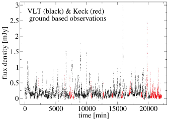
Figure 3: $K$-band light curve of Sgr A* observed with ground-based observatories. The data were taken in hours-long segments over more than a decade and are here joined together on a linear abscissa for display. Black points show data taken with VLT/NaCo at 2.18 $\mu$m (Table 2 of Witzel et al. 2012). Red points show data taken with Keck/NIRC2 (Table 4) at 2.12 $\mu$m. Flux densities are as observed with no correction for interstellar extinction. The combined $K$-band data have been used previously by Meyer et al. (2014).

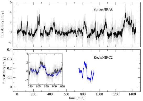
Figure 4: Observations with Spitzer/IRAC (black) and Keck/NIRC2 (blue) on 2016 July 12–13. The inset shows both light curves on an expanded abscissa and with $K$ flux density multiplied by a factor of 12.4 and then 1.74 mJy subtracted (see Appendix A and Figure 5) to match $M$. Light curves are given in observed flux density with no interstellar extinction correction. This is the only simultaneous dataset from both observatories that shows significant variability.

2.3 Simultaneous observations with NIRC2 and IRAC

A key dataset was the one on 2016 July 13, when we observed Sgr A*  with NIRC2 at 2.12 µm during IRAC 4.5 µm observations that began July 12. The AO correction for the NIRC2 dataset was comparatively poor due to the atmospheric conditions for this night, but the frames show a significant enough flux-density excursion to be taken into account in this paper. Because of the lower data quality, the standard reduction methods described above gave poor results. However, the UCLA Galactic center group developed a new software package “AIROPA” (Witzel et al. 2016) based on the PSF-fitting code StarFinder (Diolaiti et al. 2000). This package was designed to take atmospheric turbulence profiles, instrumental aberration maps, and images as inputs, and then fit field-variable PSFs to deliver improved photometry and astrometry on crowded fields. AIROPA uses improved StarFinder subroutines, in particular a much improved PSF extraction that also benefits local, static (non-field-dependent) PSF-fitting as applied to these data. Running AIROPA in static PSF mode and using the resulting PSFs to deconvolve the individual frames of 2016 July 13 improved the signal-to-noise of the light curve by a factor of three in comparison to the standard reduction. Figure 4 shows the IRAC and NIRC2 light curves.

It is remarkable how well the NIRC2 light curve is matched by the IRAC data. These two light curves impose strong limits on the $F(M)/F(K)$ ratio (from here on denoted $\Re({M}/{K})$), at least for the observed flux-density levels, which have medians of 0.15 and 0.94 mJy at $K$ and $M$ respectively . In $K$-band, this value is about 5% of the maximum flux densities seen at this wavelength. Despite confusion with the first Airy ring of the bright star S0-2 (S0-2’s closest approach to Sgr A* is anticipated for 2018), we were able to extract $K$-band fluxes at the position of Sgr A* and its vicinity with essentially zero flux density offset. In order to properly determine the offset and the flux-density ratio between the two bands, we resampled the $M$-band light curve (which has much higher cadence) to the cadence of the $K$-band light curve, and then used an MC-MC implementation in Pystan (Carpenter et al. 2017) to derive the Bayesian posteriors for the offset and the ratio while taking into account the two different measurement noise amplitudes (see Appendix A). The resulting corner plot is shown in Figure 5, and the resulting uncorrected flux-density ratio $\Re({M}/{K})=12.4\pm 0.5$. These values are the integrated ratio over the entire 204 frames and $\sim$3 hr. Instantaneous values can be even higher, and around $t=820$–825 minutes, there is a significant deviation with $\Re({M}/{K})\approx 14.7$.

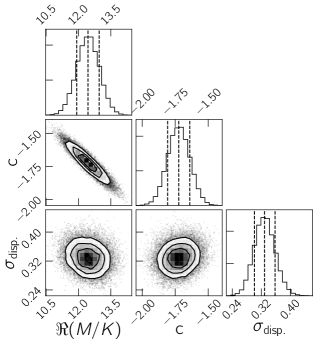
Figure 5: Results of the MCMC analysis for $\Re(M/K)$ from the simultaneous IRAC and NIRC2 data (§2.3). Contours show the joint (posterior) probability density for each parameter pair, and panels along the upper right edge show histograms of the marginalized posterior of each parameter. Parameters are the ratio $\Re(M/K)$, the dispersion $\sigma_{\rm{disp}}$ in the ratio, and the constant offset $c$.

3 Bayesian Light Curve Modeling and Results

The goal of the analysis, as it was for Hora et al. (2014), is to find the parameters that best describe the statistical variability of the observed light curves. Compared to the earlier work, the present study uses seven additional 24 hr IRAC datasets, 123 additional epochs of ground-based observations, and a more rigorous method to explore the parameter space. Simple periodograms, as shown in Figure 6, demonstrate the overall properties of the variability but do not provide the required fidelity in PSD parameter estimation. A break near 0.01 minutes^-1 is evident, but the noise does not permit a precise determination of the break frequency.

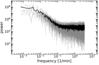
Figure 6: FFT periodograms of the eight IRAC datasets. Gray lines show the individual data sets, and the black line shows their average at each frequency. The calculation is facilitated by the IRAC light curve points being almost equally spaced in time.

The analysis method used here is simple in principle but computationally expensive. A set of statistical parameters was chosen based on prior knowledge of the variability properties. From each parameter set, many mock light curves were generated and compared to the real ones. The parameters were then modified iteratively, and new sets of mock light curves generated, seeking parameter values that minimized the differences between the real and mock data. Such an approximate Bayesian computation (ABC) gives posterior distributions for the model parameters, including proper uncertainties and correlations between the parameters, without needing an analytic likelihood function. The approximation accuracy is contingent on the selected distance function—the function that quantifies the difference between real and mock data (see Appendix B.2).

The first-order structure function $V(\tau)$ of a light curve $F(t)$ is defined as

$$V(\tau)=\langle[F(t+\tau)-F(t)]^{2}\rangle\quad,$$ (2)

that is, as the variance of the process at a given time lag $\tau$ (Simonetti et al. 1985; Hughes et al. 1992). The structure functions derived from the three datasets are shown in Figure 7.

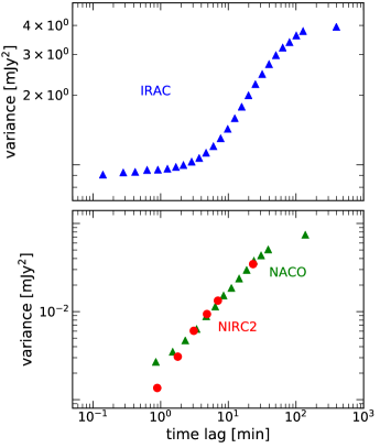
Figure 7: Logarithmically binned structure functions (Eq. 2) for the light curve data. The lower panel shows the NaCo structure function in green and the NIRC2 structure function in red. The upper panel shows the IRAC structure function.

The underlying model is based on the results of earlier analyses:

• The long-term flux-density PDF in $K$-band is a highly skewed distribution, well described by either a power law with a slope $\beta=4.2$ and a pole $F_{0}=-0.37$ mJy (Witzel et al. 2012) or by a log-normal distribution.

• The PSD has the form of a power-law with a slope $\gamma_{1}\approx 2$ and a break at a couple of hundred minutes (Do et al. 2009; Witzel et al. 2012; Meyer et al. 2014; Hora et al. 2014; Figure 6).

• The noise properties of the individual datasets are well described by Gaussians. (For the VLT and Keck data, see Witzel et al. 2012; Meyer et al. 2014; for the Spitzer data, see §2.1.)

• The uncorrected flux-density ratio for bright phases of Sgr A* $\Re(M/K)=6_{-3}^{+5}$. This corresponds to NIR spectral index $\alpha_{s}=0.6\pm 0.2$ (Hora et al. 2014; Witzel et al. 2014).

Two crucial parts of the ABC algorithm are (1) a method to simulate mock data from the model parameters, and (2) a distance function that describes how closely the mock data resemble the observed sample. Our PMC-ABC implementation, which follows that of Ishida et al. (2015), is an iterative one that first chooses random values for each of 11 parameters (listed in Table 5) according to the current probability distribution for each. (For the first iteration, the probability distribution is given by the priors.) Each parameter set is used to generate a mock light curve for NIRC2, NaCo, and IRAC, and each light curve is transformed to its structure function. For this step, the range and binning of time lags must match those of the real data.

Many structure functions are generated this way, each from new values of the 11 parameters but with the probability distributions fixed. These structure functions are compared with the structure functions of the real data via a distance function (see Appendix B). The parameter sets that give structure functions closest to the real data are used to modify the parameter probability distributions, and the cycle is repeated.

The structure function is blind to DC offsets, which is important in the context of the arbitrary flux-density zero points of the Spitzer epochs. It encodes information on the flux-density PDF, the measurement noise, the intrinsic correlations of the variability process, and the cadence and window function of the observations. (For detailed discussions of the structure function, see Emmanoulopoulos et al. 2010 and Kozłowski 2016.) The intrinsic variability process and the window function are hard to disentangle, and for our analysis it is important to choose a representation that emphasizes the parts of the structure function that are dominated by the intrinsic correlations. With increasing time lag, a decreasing number of point pairs contribute to the structure function bins. For time lags longer than half the observing window (i.e., 12 hr for Spitzer), not all flux-density measurements contribute to every structure function bin, and the variance of the structure function

Table 5: Priors and Posteriors of Bayesian analysis

		Mean of
Parameter	Prior	Posterior	Description
Case 1: $K$ power-law/$M$ power-law model
$\gamma_{1}$	flat on [1.2, 3.5]	$2.21^{+0.12}_{-0.11}$	primary PSD slope
$\gamma_{2}$	flat on [1.2, 10.0]	$6.0^{+2.8}_{-2.5}$	secondary PSD slope
$f_{b}$ [$10^{-3}\rm{minutes}^{-1}$]	flat on [1.0, 600.]	$3.50^{+0.98}_{-0.89}$	primary correlation frequency
$f_{b,2}$ [$\rm{minutes}^{-1}$]	flat on [0.001, 0.6]	$0.34^{+0.18}_{-0.16}$	secondary break frequency
		$>0.120$	$(95\%$ credible level)
$F_{0}$ [mJy]	Gaussian ($\mu=-0.36$, $\sigma=0.05$)	$-0.37^{+0.05}_{-0.05}$	pole of the power-law flux-density PDF ($K$- and $M$-band)
$\beta_{K}$	Gaussian ($\mu=4.22$, $\sigma=0.6$)	$4.53^{+0.34}_{-0.33}$	slope of the power-law flux-density PDF in $K$-band
$\beta_{M}$	Gaussian ($\mu=4.22$, $\sigma=0.6$)	$4.45^{+0.56}_{-0.56}$	slope of the power-law flux-density PDF in $M$-band
$s$	flat on [0.01, 24.0]	$5.9^{+2.5}_{-1.9}$	$M$ to $K$ flux density ratio
$\sigma_{\mathrm{Keck}}$ [mJy]	Gaussian ($\mu=0.017$, $\sigma=0.008$)	$0.014^{+0.004}_{-0.006}$	measurement noise of the Keck observations
$\sigma_{\mathrm{VLT}}$ [mJy]	Gaussian ($\mu=0.034$, $\sigma=0.008$)	$0.031^{+0.003}_{-0.003}$	measurement noise of the VLT observations
$\sigma_{\mathrm{IRAC}}$ [mJy]	Gaussian ($\mu=0.65$, $\sigma=0.2$)	$0.676^{+0.020}_{-0.019}$	measurement noise of the IRAC observations
Case 2: $K$ power-law/$M$ log-normal model
$\gamma_{1}$	flat on [1.2, 3.5]	$2.21^{+0.12}_{-0.11}$	primary PSD slope
$\gamma_{2}$	flat on [1.2, 10.0]	$6.0^{+2.7}_{-2.6}$	secondary PSD slope
$f_{b}$ [$10^{-3}\rm{minutes}^{-1}$]	flat on [1.0, 600.]	$3.71^{+1.2}_{-1.1}$	primary correlation frequency
$f_{b,2}$ [$\rm{minutes}^{-1}$]	flat on [0.001, 0.6]	$0.33^{+0.17}_{-0.16}$	secondary break frequency
		$>0.112$	$(95\%$ credible level)
$F_{0}$ [mJy]	Gaussian ($\mu=-0.37$, $\sigma=0.05$)	$-0.37^{+0.05}_{-0.04}$	pole of the power-law flux-density PDF in $K$-band
$\beta_{K}$	Gaussian ($\mu=4.22$, $\sigma=0.6$)	$4.59^{+0.32}_{-0.32}$	slope of the power-law flux-density PDF in $K$-band
$\mu_{\operatorname{logn},{M}}$	flat on [$-$6.0, 6.0]	$-0.3^{+1.3}_{-1.3}$	log-normal mean in $M$-band
$\sigma_{\operatorname{logn},{M}}$	flat on [0.001, 4.0]	$0.89^{+0.54}_{-0.50}$	log-normal standard deviation in $M$-band
$\sigma_{\mathrm{Keck}}$ [mJy]	Gaussian ($\mu=0.017$, $\sigma=0.008$)	$0.015^{+0.004}_{-0.006}$	measurement noise of the Keck observations
$\sigma_{\mathrm{VLT}}$ [mJy]	Gaussian ($\mu=0.034$, $\sigma=0.008$)	$0.031^{+0.003}_{-0.003}$	measurement noise of the VLT observations
$\sigma_{\mathrm{IRAC}}$ [mJy]	Gaussian ($\mu=0.65$, $\sigma=0.2$)	$0.678^{+0.020}_{-0.019}$	measurement noise of the IRAC observations
Case 3: $K$ log-normal/$M$ log-normal model
$\gamma_{1}$	flat on [1.2, 3.5]	$2.10^{+0.10}_{-0.09}$	primary PSD slope
$\gamma_{2}$	flat on [1.2, 10.0]	$5.8^{+2.8}_{-2.4}$	secondary PSD slope
$f_{b}$ [$10^{-3}\rm{minutes}^{-1}$]	flat on [1.0, 600.]	$4.11^{+0.76}_{-0.65}$	primary correlation frequency
$f_{b,2}$ [$\rm{minutes}^{-1}$]	flat on [0.001, 0.6]	$0.31^{+0.19}_{-0.15}$	secondary break frequency
		$>0.118$	$(95\%$ credible level)
$\mu_{\operatorname{logn},{K}}$	flat on [$-$8.3, 3.7]	$-1.35^{+0.62}_{-0.60}$	log-normal mean in $K$-band
$\sigma_{\operatorname{logn},{K}}$	flat on [0.001, 4.0]	$0.56^{+0.24}_{-0.21}$	log-normal standard deviation in $K$-band
$\mu_{\operatorname{logn},{M}}$	flat on [$-$6.0, 6.0]	$1.01^{+0.47}_{-0.44}$	log-normal mean in $M$-band
$\sigma_{\operatorname{logn},{M}}$	flat on [0.001, 4.0]	$0.39^{+0.15}_{-0.13}$	log-normal standard deviation in $M$-band
$\sigma_{\mathrm{Keck}}$ [mJy]	Gaussian ($\mu=0.017$, $\sigma=0.008$)	$0.013^{+0.005}_{-0.006}$	measurement noise of the Keck observations
$\sigma_{\mathrm{VLT}}$ [mJy]	Gaussian ($\mu=0.034$, $\sigma=0.008$)	$0.030^{+0.002}_{-0.003}$	measurement noise of the VLT observations
$\sigma_{\mathrm{IRAC}}$ [mJy]	Gaussian ($\mu=0.65$, $\sigma=0.2$)	$0.677^{+0.013}_{-0.013}$	measurement noise of the IRAC observations

increases dramatically without carrying much information about the intrinsic variability. Therefore we chose a logarithmic binning scheme, roughly equally spaced in logarithmic time lags, with a spacing large enough to allow for a similar number of points in the long-time-lag bins. We included time lags up to half the size of the observing window, $\sim$700 minutes in the case of the IRAC data. For the NaCo and the NIRC2 data, which have a wide range of observing window durations, we used points of similar variance increase in the structure function, 300 minutes and 40 minutes, respectively. For the ranges of [160, 700] minutes (IRAC), [50, 300] minutes (NaCo), and [10.5, 40] minutes (NIRC2), we used a single large bin with three times the weight in the distance function as the lower bins (see Equation Appendix B9). This approach makes conservative use of the complementary but overlapping information provided by each instrument, with IRAC providing the longest timescales covering the coherence timescale, NaCo at medium timescales between 100 and 10 minutes, and NIRC2 at the shortest timescales to below 1 minute.

The slope of the structure function is related to the slope of the underlying PSD but is also a function of the overall variance of the process and the variance of the measurement noise. In particular, for red noise with quickly decreasing amplitudes toward higher frequencies, the structure function at the shortest timescales close to the data cadence $\tau_{\rm{cad}}$ is

$$V(\tau\approx\tau_{\rm{cad}})\approx 2\sigma^{2}\quad,$$ (3)

with $\sigma$ the measurement noise. If the red-noise process has finite variance, then at timescales much larger than the coherence timescale $\tau_{b}$, the structure function is

$$V(\tau\gg\tau_{b})\approx 2\cdot{\rm Var}[F(t)]+2\sigma^{2}\quad,$$ (4)

with ${\rm Var}[F(t)]$ the variance of the variability process.

Ishida et al. (2015) implemented ABC sampling in Python and gave a detailed description of the method. Following their approach, we developed our own C++ implementation. Appendix B gives a more detailed description of the algorithm and the underlying model.

We tested three models of the flux density PDFs:

• Case 1 : independent power-law parametrizations of the flux-density PDFs in $K$-band and $M$-band

• Case 2 : a power-law parametrization of the flux-density PDF in $K$-band and a log-normal parametrization in $M$-band

• Case 3 : independent log-normal parameterizations of the flux-density PDFs in $K$- and $M$-band while including $\Re(M/K)=12.4\pm 0.5$ from the synchronous $K$- and $M$-band data (Section 2.3)

All of the above parametrizations describe the data in the limited flux-density range observed, and at least in the $K$-band, they are equally valid. The choices were informed by the analyses of Dodds-Eden et al. (2011) and Witzel et al. (2012). While a log-normal distribution can be expected from accretion variability processes (e.g., Uttley et al. 2005), and indeed a log-normal distribution can also describe the observed $K$-band flux densities, the log-normal parameters derived are related to the location of the mode of the PDF. For the NaCo data, which constitute the majority of the $K$-band data, the mode is close to the white-noise-dominated part of the distribution. This makes both parameters difficult to determine with precision. In contrast, power-law parameters—slope and normalization—describe mainly the tail, which is well above the white noise. For $K$-band, Witzel et al. (2012) showed that the power-law description is advantageous, but it makes the simplifying (and possibly unphysical) assumption a sharp cutoff at zero flux density. Nevertheless, the baseline Case 1 fit uses a power law for both bands. Because we do not have, a priori, a detailed understanding of the $M$-band distribution, and also motivated by additional information drawn from synchronous data, Case 2 investigates a log-normal distribution for $M$-band. Finally, adding constraints from simultaneous $K+M$ data lets even the double log-normal parametrization give well-constrained parameters, and Case 3, our preferred model, gives results for this possibility.

To simultaneously fit the structure functions of the three datasets, the model parameters (Table 5) are as follows:

• in all cases the respective instrumental measurement uncertainties $\sigma$ and four PSD parameters: slopes $\gamma_{1}$ and $\gamma_{2}$ and break frequencies $f_{b}$ and $f_{b,2}$;

• for Case 1, flux-density PDF parameters $F_{0}$ (pole), $\beta_{K}$ and $\beta_{M}$ (power-law slopes), and the $M$- to $K$-band ratio factor $s$;

• for Case 2, $K$ power-law parameters $F_{0}$ (pole) and $\beta_{K}$ and $M$ log-normal parameters $\mu_{\operatorname{logn},{M}}$ and $\sigma_{\operatorname{logn},{M}}$.

• for Case 3, two pairs of log-normal parameters $\mu_{\operatorname{logn},{K}}$, $\sigma_{\operatorname{logn},{K}}$, $\mu_{\operatorname{logn},{M}}$, and $\sigma_{\operatorname{logn},{M}}$. The Case 3 analysis is additionally based on a modified distance function (Equation Appendix D5) to select combinations of log-normal PDFs that result in $\Re[M/K,F(K)=0.15~{}\rm{mJy}]\approx 12.4$ (see Section 4.4 for details).

Table 5 lists the priors for each of the parameters

Developing and running the ABC algorithm required an extensive effort in optimization of code and adaptation of the distance function to the problem to achieve the results presented here. The large number of calculations involved in the massive iterative generation and evaluation of light curves—including both test and final analysis runs—required in total about 60,000 CPU hours on our UCLA Hoffman cluster node and 250,000 CPU hours on the XSEDE super clusters Stampede1, Comet, and Bridges (Towns et al. 2014). Each of the runs reported here took 2 days on 24 cores, and the last iteration with 10,000 parameter sets took about 1 day each on 800–1200 cores executing ${\sim}2\times 10^{10}$ FFTs. The results of our Bayesian analyses are shown in Figures 8, 9, and 10, and the weighted averages and standard deviations are listed in Table 5.

Figure 8: Results of the Bayesian structure function fit for Case 1 (power-law/power-law; see §3). Contours show the joint (posterior) probability density for each parameter pair, and panels along the upper right edge show histograms of the marginalized posterior of each parameter defined in Table 5. The upper limit for $1/f_{b,2}$ with a probability of 95% is 8.3 minutes.

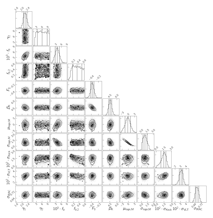
Figure 9: Results of the Bayesian structure function fit for Case 2 (power-law/log normal: see §3). Contours show the joint (posterior) probability density for each parameter pair, and panels along the upper right edge show histograms of the marginalized posterior of each parameter defined in Table 5. The upper limit for $1/f_{b,2}$ with a probability of 95% is 8.6 minutes, nearly the same as Case 1. The strong correlation between the $M$ log-normal parameters is expected when the mode of the intrinsic log-normal distribution below the white noise level.

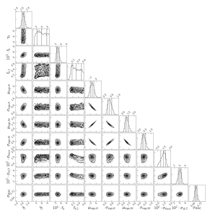
Figure 10: Results of the Bayesian structure function fit for Case 3 (log-normal/log-normal; see §3). Contours show the joint (posterior) probability density for each parameter pair, and panels along the upper right edge show histograms of the marginalized posterior of each parameter defined in Table 5. The upper limit for $1/f_{b,2}$ with a probability of 95% is 8.5 minutes, about the same as Cases 1 and 2.

For Case 1 (power-law/power-law), all parameters are well constrained with the exception of the secondary break frequency $f_{b,2}$ and slope $\gamma_{2}$. The secondary break frequency has a lower limit $f_{b,2}>0.120~{}\rm{minutes}^{-1}$ or equivalently an upper limit for the secondary break timescale of 8.3 minutes at the 95% credible level. The main break timescale $\tau_{b}=286^{+191}_{-94}$ minutes (90% credible level).

For Case 2 (power-law/log-normal), all parameters are similarly well constrained, again with the exception of the secondary break frequency and slope. The limit is $f_{b,2}>0.112~{}\rm{minutes}^{-1}$ or equivalently an upper limit for the secondary break timescale of 9.0 minutes (95% credible level). The main break timescale $\tau_{b}=270^{+261}_{-92}$ minutes ($90\%$ credible level).

For Case 3 (log-normal/log-normal), again all parameters but the secondary break frequency $f_{b,2}$ and slope $\gamma_{2}$ are well constrained. The limit is $f_{b,2}>{0.118}$ minutes^-1 or equivalently an upper limit for the secondary break timescale of 8.5 minutes (95% credible level). The main break timescale $\tau_{b}=243^{+82}_{-57}$ minutes (90% credible level).

4 Discussion

4.1 Validation of the distance function

4.2 Quality of the statistical analysis

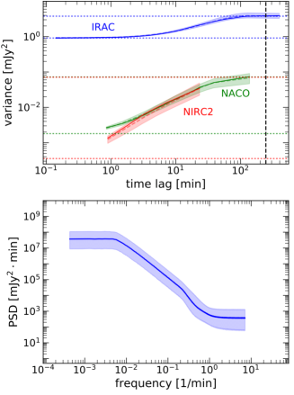
Figure 11: Structure functions and power spectral density. The upper panel shows structure functions (Eq. 2) for the three instruments. Solid lines show the observed data (as presented in Figure 7), and corresponding dashed curves show the median of 10,000 Case 3 (see §3) model structure functions for the respective instruments. The shaded envelopes denote the model $68\%$ credible intervals for each time lag. The vertical dashed line marks the derived correlation timescale $1/f_{b}$. Pairs of horizontal short-dashed lines, color-coded for each instrument, mark the two noise levels of each measurement. The lower line of each pair indicates the measurement noise (Eq. 3), and the upper line the intrinsic red noise of the Sgr A* variability when sampled at timescales ${\gg}\tau_{b}$ combined with measurement noise (Eq. 4). (The upper lines for NaCo and NIRC2 are nearly indistinguishable.) The details of generating the structure functions, including the choice of time lag ranges, are described in §3 and Appendix B.2. The slope of the structure function relates to the slope of the PSD but also depends on the underlying white noise level and is therefore different for each observatory despite the common PSD. The lower panel shows power spectral densities of 10,000 mock IRAC light curves derived from the final Case 3 parameters. The mock light curves have the same cadence as the IRAC data but the lower white noise of the NIRC2 data. The solid line shows the median for each frequency, and the shaded areas show the $68\%$ credible intervals. Because the PSD is a function of frequency, short time lags are to the right. The units of the PSD are $\rm{mJy}^{2}\cdot\rm{minutes}$, but the scaling of PSD values shown here is arbitrary. The slight break in slope around 0.2 minutes^-1 is well within the 1$\sigma$ envelope. It arises from the condition $\gamma_{2}>\gamma_{1}$ and the lack of sensitivity to structure below 9 minutes, close to the white noise level.

The mock structure functions resulting from the derived posterior distributions (Table 5) are in excellent agreement with the observed structure functions. Based on the final Case 3 iteration, we created 10,000 structure functions for each instrument, and these closely resemble the measured structure functions as shown in the upper panel of Figure 11. This figure additionally shows the short- and long-timescale white noise levels of the processes (see Equations  3 and 4). The latter were directly derived from the Case 3 log-normal parameters. The measured structure functions asymptotically approach the calculated levels.

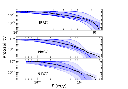
Figure 12:

4.3 Power spectral density of NIR variability

Based on our combined modeling of the PSD and the flux-density PDFs (and in Case 3 the additional constraints from $K$- to $M$-band spectral properties), we can derive a well-constrained estimate of the PSD of the Sgr A* NIR variability. The lower panel of Figure 11 shows a PSD synthesized from the final Case 3 parameters. This synthesized PSD shows a well-constrained shape over three orders of magnitude in frequency. The IRAC data fully cover the coherence timescale of the variability process (as expected), and there is no significant evidence for a second break timescale below 20 minutes. However, FFT periodograms on real data with white noise and irregular sampling are not statistically consistent estimators and not well suited for precision measurements of the PSD parameters, motivating our use of the ABC sampler. The coherence timescale for Case 1 is $\tau_{b}\equiv 1/f_{(b)}=286^{+191}_{-94}$ minutes at the $90\%$ credible level. Case 2 gives much the same timescale $\tau_{b}=270^{+261}_{-92}$ minutes but with a larger uncertainty because of the uncertainty in the log-normal parameters. Case 3 shows a slightly different (but consistent within 1$\sigma$) and more precise $\tau_{b}=243^{+82}_{-57}$ minutes. The validity of the smaller error bars is dependent on whether or not one considers $\Re({M}/{K})$ derived from the synchronous data as representative of the true ratio at that flux density. All three cases give the most precise determination of the PSD parameters so far, and all are consistent with the earlier estimate $\tau_{b}=128^{+329}_{-77}$ minutes (Meyer et al. 2009). Figure 13 compares the credible contours of the respective analyses.

Break timescales of several hours are consistent with viscous timescales rather than with dynamical timescales (e.g., orbital modulations due to inhomogeneities in the accretion flow; Dexter et al. 2014). Dexter et al. analyzed the characteristic timescale of Sgr A* from 230, 345, and 690 GHz submm data and found $\tau_{b,\rm{submm}}=480^{+180}_{-240}$ minutes at the 95% credible level. The authors pointed out that the timescale of $\sim$8 hr in the submm is more than $3\sigma$ larger than the NIR timescale of $\sim$2.5 hr (Meyer et al., 2009). Dexter et al. 2014 discussed the possibility of the NIR emission originating from the same process as the submm but at smaller radii. The dependence of the viscous timescale on the radius is $t_{\rm{visc}}\propto R^{3/2}$. Therefore the timescales above suggest the NIR radius to be $\sim$0.5 of the submm radius. For a canonical size $R_{\rm{submm}}=3R_{S}$ of the submm emission region (with $R_{S}$ the Schwarzschild radius), this puts the NIR emitting process very close to the ISCO (which is unlikely). The authors concluded that a difference in radius is likely not the reason for the different timescales and suggested that adiabatically expanding plasma with delayed submm emission at larger sizes could be a natural explanation of the timescales.

Our findings change the interpretation of the relative timescales. $\tau_{b,\rm{NIR}}=243^{+82}_{-57}$ minutes is statistically consistent with the submm values. This suggests a more direct relation between the NIR and submm emission (e.g., both wavelengths stemming from the same optically thin synchrotron source). A detailed analysis of a larger submm dataset with similar statistical tools as used here and further simultaneous observations are needed to refine this relation.

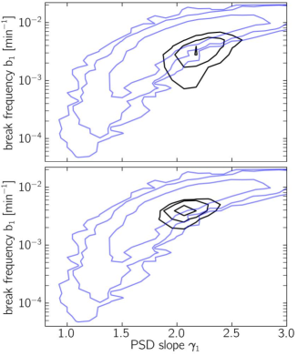
Figure 13: Credible contours ($68\%,95\%,99\%$) for the parameters $\gamma_{1}$ and $f_{b}$ (Table 5). The upper panel shows Case 1 and the lower panel shows Case 3. The blue contours are from Figure 3 of Meyer et al. (2009), and the black contours show results of the present analysis. The posteriors have been marginalized over all other parameters.

Despite the ability of the ABC algorithm to detect secondary timescales in mock data, there is little indication of a second break in the real data, regardless of the choice of parametrization. Indeed, a second break can be restricted to timescales $<$9 minutes. Only Case 3 has even a small peak in the posterior with $1/f_{b,2}\approx 6$ minutes. (See the $f_{b,2}$ histogram in Figure 10.) Shorter break times are consistent with the data, and the secondary break slope $\gamma_{2}$ is unconstrained. The existing data therefore do not require a second break at all.

Several models predict modulation of the NIR light at frequencies related to motion at the innermost stable circular orbit (ISCO) of the black hole, either as a QPO (Meyer et al., 2006a; Zamaninasab et al., 2010; Dolence et al., 2012) or a loss of PSD power below the ISCO timescale. Either would create a second break (Dolence et al. 2012). If these or other processes near the ISCO modulate the light curve of Sgr A*, the absence of a secondary break in the PSD implies a lower limit on the black hole spin. The orbital period for a direct-rotation, equatorial orbit at the ISCO is

$$P=2\pi(x_{\rm{ISCO}}^{3/2}+a)\frac{GM_{bh}}{c^{3}}$$ (5)

where $0\leq a<1$ is the dimensionless black hole spin, and $x_{\rm{ISCO}}$, the radius of the ISCO in units of $GM_{bh}/c^{2}$, is given by

$$x_{\rm ISCO}=3+Z_{2}-[(3-Z_{1})(3+Z_{1}+2Z_{2})]^{1/2}.$$ (6)

Here $Z_{1}\equiv 1+(1-a^{2})^{1/3}[(1+a)^{1/3}+(1-a)^{1/3}]$ and $Z_{2}\equiv(3a^{2}+Z_{1}^{2})^{1/2}$ (Bardeen et al. 1972). Figure 14 shows $P(a)$ for $M_{bh}=4\times 10^{6}\ \rm{M}_{\odot}$. Only ISCO modulation periods shorter than the 9 minute upper limit and therefore black hole spins $a>0.9$ are consistent with the light curve data, unless there are no NIR flux variations at the frequency of the ISCO. The hint of a posterior peak for case 3 at about 6 minutes would, if taken seriously, point to maximum spin if the power is generated at the ISCO. The models as presented by, for example, Meyer et al. (2006a, 2007) and Zamaninasab et al. (2010) can be ruled out because they predict NIR variability with typical timescales of 15–20 minutes.

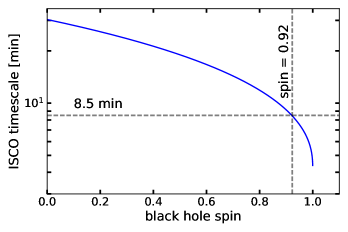
Figure 14: ISCO orbital period (Eq. 5) as a function of black hole spin in the Kerr metric for a black hole mass $4\cdot 10^{6}$ ${M}_{\odot}$. The horizontal dashed line indicates a period of 8.5 minutes, the upper limit on a secondary break timescale. The vertical dashed line shows the corresponding dimensionless spin $a$.

4.4 Sgr A*’s NIR spectral index

The $K$- to $M$-band ratio derived from the Case 1 (power-law/power-law) ABC fit $s=5.9^{+2.5}_{-1.9}$ ($1\sigma$) is in excellent agreement with the value $s=5.8^{+4.8}_{−2.9}$ calculated from the published NIR source spectral index $\alpha_{s}=0.6\pm 0.2$. That index was derived from synchronous 1.6 $\mu$m to 3.7 $\mu$m measurements (Hornstein et al. 2007; Witzel et al. 2014). However, $s\approx 6$ is in striking disagreement with $\Re({M}/{K})\approx 12$ derived from the simultaneous $K$ and $M$ data during its particularly dim flux-density level with a median of $F(K)=0.15$ mJy (Section 2.3).

In order to test how $s\approx 6$ is related to our choice of prior, we attempted to alter the prior such that a higher value of $s$ was preferred. In all tests with Gaussian priors centered around $s>6.0$, the ABC sampler consistently found a posterior about $1\sigma$ below the mean value of the prior to approach $s=6.0$. Altering the prior for $s$ to exclude $s=6.0$ and prefer higher values led to significantly different power-law indices $\beta$ for the flux-density PDFs in the two bands (and thus to a flux-density-dependent spectral index; see Appendix D). In the case of flat priors wide enough to encompass $s=6.0$, the ABC code always reverted to a posterior $s\approx 6.0$ (Figure 8). This behavior shows that, integrated over the entire datasets and in the absence of simultaneous data, $s=6.0$ describes the data well enough to match the total variance in both bands (i.e., the levels and shapes of the structure functions at longer time lags).

The tension between the statistically derived ratio $s$ and the observed ratio suggests a variable spectral index, in particular a trend of $\alpha_{s}$ with flux-density level. All three parametrizations allow the NIR spectral index to be a function of flux-density level. Based on the fact that the light curves at different wavelengths within the NIR are almost identical in shape (ignoring the minor short-timescale fluctuations discussed in Section 2.3 and Witzel et al. 2014), the basic assumption is that if one NIR band rises or falls, the other rises or falls too. As a consequence, the quantiles of the flux-density PDFs must be equal for corresponding flux densities, and it is possible to derive the flux-density ratio between two bands as a function of flux density in one of the bands and the PDF parameters. These dependencies are calculated in Appendix D for our three different combinations of power-law and log-normal PDFs. In Case 1 our posterior distributions for $F_{0}$, $\beta_{K}$, $\beta_{M}$, and $s$ result in an almost perfectly constant $\Re({M}/{K})$ independent of $F_{K}$. This is expected because the posteriors of the power-law slopes $\beta_{K}$ and $\beta_{M}$ are almost identical, and the PDFs in both bands are the same except for a factor $\Re({M}/{K})\approx s$.

In the context of matching quantiles, larger values for $\Re({M}/{K})$ at low flux-density levels imply different distributions for $K$ and $M$-band flux densities, in particular a flattening of the $M$-band flux-density PDF toward low flux densities relative to the $K$-band PDF. The IRAC dataset is competitive with the S/N of the ground-based telescopes (Hora et al. 2014). The measured large value for $\Re({M}/{K})$ is an indicator that, in contrast to $K$-band, in $M$-band we start to discern the intrinsic turnover at the mode of the flux-density PDF despite measurement noise. Dodds-Eden et al. (2011) originally suggested a log-normal flux-density PDF parametrization for Sgr A*. Parameterizing the $M$-band PDF as a log-normal while keeping the power-law parametrization for $K$-band (as a well-constrained reference) is one way to test for the presence of an intrinsic turnover in the $M$-band PDF. Case 2 analyzes this possibility.

Figure 15 illustrates how the different $K$ and $M$ PDFs lead to a variable flux-density ratio that naturally reaches $\Re({M}/{K})=12.4$ at the average offset-corrected flux density $F_{\rm{avg}}=0.15$ mJy measured for the 2016 data. Unfortunately, because the log-normal parameters cannot be well constrained from non-synchronous data only, the marginalized distribution of the flux density ratios is much wider in Case 2 than in Case 1 (Figure 15). At low flux densities, the 1$\sigma$ and 2$\sigma$ contours cover a huge range of possible flux-density ratios. However, the distributions peak at about the same ratio, and the flux-density ratio at high flux densities is about the same in both cases. This suggests that the power-law/log-normal parametrization of Case 2 can naturally explain both the redder spectral indices observed for low phases of Sgr A* (Eisenhauer et al. 2005; Gillessen et al. 2006; Krabbe et al. 2006; Bremer et al. 2011; Ponti et al. 2017) and the bluer spectral indices during brighter phases (Ghez et al. 2005b; Hornstein et al. 2007; Bremer et al. 2011; Witzel et al. 2014).

This discussion takes $\Re({M}/{K})\approx 12$ at face value despite evidence for short-timescale fluctuations. However, this value is integrated over $\sim$3 hr during which the source fluctuated around the low level of $F_{K}\sim 0.15$ mJy with a maximal variation amplitude of $\Delta F_{K}\approx 0.1$ mJy. In the following, we assume that this ratio is representative for $F_{K}\approx 0.15$ mJy.

In Case 3 we assumed a log-normal parametrization for both bands. (It would be surprising for the $K$-band PDF to have a fundamentally different form than the $M$-band PDF.) This case exploits the additional information from the synchronous data in our statistical analysis of the non-synchronous datasets. This is achieved by a modification of the distance function, as given by Equation Appendix D5. This approach has immense constraining power and allows us to derive tight posteriors for the log-normal parameters of both bands. Equation Appendix D4 gives $\Re({M}/{K})$ as a function of $F(K)$ as derived from the posteriors. Figure 16 shows the drastic improvement of the 1$\sigma$ and 2$\sigma$ envelopes. Interestingly, the flux density distributions derived from the posteriors predict $F(K)\leq 0.15$ mJy to occur with a probability of only $\sim$23% (this flux density is located left of the peak of most distributions ), and the flux-density-ratio histogram in the range directly observed is peaked around $\Re({M}/{K})\approx 9.0$, close to the value derived in Case 1.

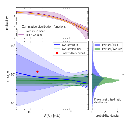
Figure 15: Flux-density ratio $\Re(M/K)$ as a function of $K$-band flux density, as derived from our posteriors for Cases 1 and 2. The central panel shows the median and 68% and 95% credible contours for Case 1 in green and for Case 2 in blue. The red point denotes the flux-density ratio derived from the simultaneous observations (§2.3). The upper panel shows the CDFs for Case 2: $M$-band in purple and $K$-band in orange. Shading indicates the limits at the 68% credible level. In order to make the CDFs comparable, the abscissa of the $M$-band CDF (i.e., the $M$-band flux densities) has been scaled by a factor 1/5.9 (with 5.9 being the average $\Re(M/K)$ in Case 1) to place them on the same scale as the $K$-band flux densities. The right panel shows histograms of $\Re(M/K)$ marginalized over the actually observed flux-density range. Case 1 is in green and Case 2 in blue.

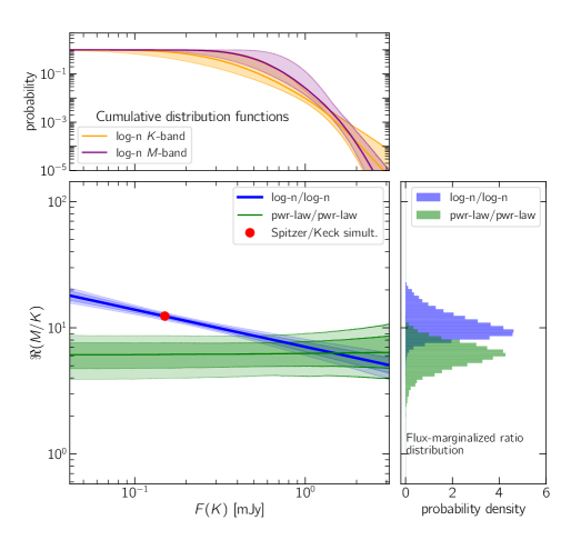
Figure 16: Flux-density ratio $\Re(M/K)$ as a function of $K$-band flux density for Case 3. The central panel shows the median and 68% and 95% credible contours for Case 1 in green and for Case 3 in blue. The red point denotes the flux-density ratio derived from the simultaneous observations (§2.3). The upper panel shows the CDFs for Case 3: $M$-band CDF in purple and $K$-band CDF in orange. Shading indicates the 68% credible intervals. In order to make the CDFs comparable, the abscissa of the $M$-band CDF (i.e., the $M$-band flux densities) has been scaled by a factor 1/5.9 (with 5.9 being the average $\Re(M/K)$ in Case 1) to place them on the same scale as the $K$-band flux densities. The right panel shows histograms of $\Re(M/K)$ marginalized over the actually observed flux-density range. Case 1 is in green and Case 3 in blue.

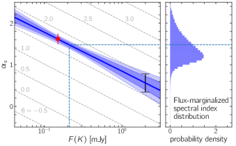
Figure 17: $K$-band to $M$-band spectral index as a function of $K$-band flux density. The filled red circle in the left panel shows the result of the simultaneous data (Fig 4), and the solid line shows the relation from Equation 7 with parameter posteriors of Case 3. Shaded areas show the 68% and 95% credible contours. Absolute values of $\alpha_{s}$ are based on extinctions $A_{K}=2.46$ mag and $A_{M}=1.0$ mag, . The right panel shows the histogram of $\alpha_{s}$ marginalized over the actually observed flux-density range. The dashed lines show (vertical) the typical flux-density level and (horizontal) the corresponding $\alpha_{s}$. Previous studies (e.g., the Hornstein et al. 2007 determination of $\alpha_{K-L}$) became noise dominated below $\sim$0.2 mJy. Gray curves show (Equation Appendix E8) for several values of $\tilde{\eta}$ as labeled.

In summary, in all three cases $\Re({M}/{K})$ at high flux density is consistent with $\alpha_{s}\approx 0.6$ (e.g., Hornstein et al. 2007 and reddening values from Section 1). At $F(K)=0.15$ mJy, $\alpha_{s}=1.64\pm 0.06$. This is the most precise determination of a spectral index change with flux density in the existing literature. This value is consistent with $\alpha_{s}=1.7$ determined by Gillessen et al. (2006) for their off-state-subtracted dim state. The combined data are consistent with well-constrained log-normal parameters for both $M$ and $K$ and require $\alpha_{s}$ to depend on the flux-density level. For Case 3, an empirical equation for $\alpha_{s}$ as a function of observed $F(K)$ is

$$\begin{split}\alpha_{s}=\xi\cdot\log{\bigg{[}\frac{F(K)}{\rm{mJy}}\bigg{]}}+\eta+1.2708\cdot(A_{M}-A_{K})\quad,\end{split}$$ (7)

with $\xi=-0.93\pm 0.16$ and $\eta=2.7\pm 0.1$ (1$\sigma$ uncertainties). Equation Appendix D8 shows how Equation 7 was derived, and Figure 17 illustrates the resulting $\alpha_{s}$ dependence on flux density. The correlation between $\xi$ and $\eta$ is $\rho(\xi,\eta)=C(\xi,\eta)/(\sigma_{\xi}\sigma_{\eta})=0.87$ (with $C(\xi,\eta)=0.0115$ the cross-covariance) – that is, the two parameters are strongly correlated. For $F(K)<0.35$ mJy, Case 3 predicts a deviation of more than $2\sigma$ .

The change of $\alpha_{s}$ with flux density is in the same direction but less extreme than found by Eisenhauer et al. (2005), Krabbe et al. (2006), or Ponti et al. (2017). A direct comparison between the studies is difficult because of the following:

• Different $S/N$ from the various instruments; for Gaussian white measurement noise, $\alpha_{s}$ at low, noise-dominated flux densities becomes the logarithm of a Cauchy-distributed random variable (i.e., a distribution with extreme tails in both directions)

• Different levels of background contamination and different methods of background subtraction

• Intrinsic momentary variations outside the general trend (which we determined here with integral methods; e.g., the simultaneous $K$ and $M$ data presented here show an extreme value of $\alpha_{s}\geq 1.9$ in one brief time interval)

The present analysis benefits from two advantages: (1) The comparably high S/N in both bands thanks to the IRAC $M$-band data. (2) The determination of $\alpha_{s}$ from flux-density PDFs, which themselves are derived from structure functions (i.e., from flux-density differences rather than from absolute flux-density levels). Background contamination is only an issue for the simultaneous dataset, which is one of the longest Keck light curves available and which has a distinct shape. That makes the determination of the offset and the flux-density ratio very accurate.

The intrinsic short-timescale variations of $\alpha_{s}$ seem to be based on small flux-density deviations of one band relative to the shape of the other. As a consequence, they significantly change the spectral index only at low flux-density levels. As the flux-density levels rise, the spectral index should follow the trend of Equation 7 with increasing precision. A simple comparison with the Hornstein et al. (2007) and Witzel et al. (2014) data suggests consistency with such a mild trend. An in-depth analysis of additional data will be published separately.

4.5 Implications of the flux-density-dependent spectral index for a radiative model

For the parametrization of Case 3, we can provide a physical context why the spectral index is a linear function of $\log{\left[F(K)\right]}$. In the following we analytically compare our results to the submm/NIR variability model discussed by Eckart et al. (2006b) and Bremer et al. (2011). Eckart et al. (2006b) argued that the submm ($>$1 THz) to NIR emission is pure synchrotron radiation or synchrotron radiation with an additional contribution from synchrotron self-Compton emission. During brighter phases of Sgr A*, $\alpha_{s}=0.6$ is close to the canonical value for optically thin synchrotron radiation ($\alpha_{s}=0.7$; e.g., Moffet 1975). The turnover of the synchrotron spectrum from optically thick to optically thin is assumed to be at frequencies $\lesssim$1 THz. The steeper spectral indices during dim phases discussed in the literature (Ghez et al. 2005a; Eisenhauer et al. 2005; Gillessen et al. 2006; Krabbe et al. 2006) are interpreted as the result of a changing electron energy distribution with a changing exponential cutoff at high energies due to synchrotron losses. As derived in Appendix E, the dependence of $\alpha_{s}$ on $S(\nu)$ is :

$$\alpha_{s} = \tilde{\xi}\cdot\log{\left[\frac{S(\nu)}{\rm{mJy}}\right]}+\tilde{\eta}\quad,$$ (8)

with $\tilde{\xi}$ and $\tilde{\eta}$ being parameters related to the observing frequencies and submm spectral index and defined in Appendix E. Equation 8 has the same form as Equation 7, and one can see this as a motivation to use the log-normal/log-normal parametrization in the context of this model. With $\nu_{1}=6.66\times 10^{13}$ Hz ($M$-band) and $\nu=\nu_{2}=1.375\times 10^{14}$ Hz ($K$-band), $\tilde{\xi}=-0.96576\approx\xi$, i.e., the spectral index slope for this model is in excellent agreement with the empirical slope determined in Case 3. This is illustrated in Figure 17. Equations Appendix E5 and 7 give for the break-off frequency $\nu_{0}$

$$\frac{\nu_{0}}{\rm{THz}} = 24.1921\cdot\Bigg{\{}\tilde{\alpha}_{s}-\xi\cdot\log{\bigg{[}\frac{F(K)}{\rm{mJy}}\bigg{]}}$$ (9)

$$-\eta-1.2708\cdot(A_{M}-A_{K})\Bigg{\}}^{-2}\quad,$$

with the condition

$$\log{\bigg{[}\frac{F(K)}{\rm{mJy}}\bigg{]}}<\left[\frac{\tilde{\alpha}_{s}-\eta-1.2708\cdot(A_{M}-A_{K})}{\xi}\right].$$ (10)

This last inequality states that $\tilde{\alpha}_{s}$, can only be constant for a certain flux range (e.g., $0~{}\rm{mJy}<F(K)<3.0~{}\rm{mJy}$ for $\tilde{\alpha}_{s}=0.4$). For flux densities higher than this range, $\tilde{\alpha}_{s}$ needs to become smaller.

Figure 18 shows $\nu_{0}$ as a function of $F(K)$ in the range of 0.4–1.5 mJy for a constant, optically thin spectral index $\tilde{\alpha}_{s}=0.4$ and at a submm frequency $\tilde{\nu}=1$ THz. The required flux-density of the optically thin submm component is $\sim$2.3 Jy for $\tilde{\alpha}_{s}=0.4$. This value is similar to, but somewhat smaller than, the typical submm levels, which indicates that such an optically thin submm component might not account for all submm radiation. The predicted cutoff frequencies for moderately bright phases in the NIR are between $50$ THz and $200$ THz. Equations Appendix E10 and 10 leave open the possibility for a rich interdependence of $F(K)$, $S(\tilde{\nu})$, and $\tilde{\alpha}_{s}$ that is testable with synchronous observations. Indeed, a close correlation between submm fluctuations seen with SMA and the 2014 June 18 IRAC light curve has been observed (Fazio et al., 2018). However, other studies have found evidence for optically thick synchrotron radiation at submm wavelengths (e.g., Yusef-Zadeh et al. 2008). The simple model only begins to address the question of how the NIR and an optically thin submm component might be related. It does not provide any explanation about the origin of the variability in the submm, the origin of the non-thermal electrons, the acceleration mechanisms, or the link to the X-rays, which are crucial for understanding the high energy end of the electron distribution (see, e.g., Ponti et al. 2017).

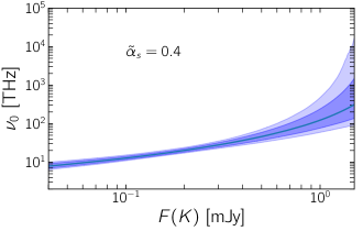
Figure 18: Synchrotron cutoff frequency as a function of observed $K$-band flux density according to Eq. 9 for $\tilde{\alpha}_{s}=0.4$. Solid lines show the median and shaded areas the 68% and 95% credible contours.

4.6 The Sgr A* spectral energy distribution

In Case 3, the inferred log-normal parameters allow us to derive the mode and the expected flux-density PDF for each band. These quantities provide information on the lower limits of NIR flux densities. The modes of the log-normal distributions are

$$\mathcal{M}[F(M)] = 2.34^{+1.75}_{-1.04}~{}\rm{mJy}~{}~{}\rm{and}$$

$$\mathcal{M}[F(K)] = 0.19^{+0.24}_{-0.11}~{}\rm{mJy}$$ (11)

for the $M$- and $K$-band, respectively. With a Galactic center distance of 8.3 kpc (and extinctions given in Section 1), these flux densities correspond to

$$\mathcal{M}(\nu_{M}L_{\nu_{M}}) = (3.2^{+2.4}_{-1.4})~{}10^{34}~{}\rm{erg}~{}\rm{sec}^{-1}~{}~{}\rm{and}$$

$$\mathcal{M}(\nu_{K}L_{\nu_{K}}) = (2.6^{+2.0}_{-1.2})~{}10^{34}~{}\rm{erg}~{}\rm{sec}^{-1}\quad.$$ (12)

The error bars do not include uncertainties in the extinction or distance. These values are in full agreement with previously published upper limits (Genzel et al. 2003 and references therein).

In order to put the NIR flux densities in context, it is important to understand how the SED was estimated in the radio regime. The radio levels were obtained as average flux densities of multiple observations (e.g., Falcke et al. 1998). Because of the symmetry of the intrinsic flux-density PDFs in the radio regime, the average is identical with the mode. The NIR modal values, being the most probable flux densities of Sgr A* during its least variable moments, are the natural counterparts to these radio flux density levels and can be interpreted as characteristic flux densities of Sgr A* within their bands. In this picture, a distinction between a quiescent (or steady) and a variable NIR state, as often proposed in the literature, is unnecessary. The modal values are merely particular flux densities within the distributions of variable flux densities.

Despite its attractive simplicity, representing the variable flux densities of Sgr A* by a single value is misleading. A full characterization of flux densities is provided by the expected flux-density PDF. This PDF incorporates information on both the intrinsic variability and the uncertainty in the parameters of the log-normal distributions given our data, and therefore is the proper tool for comparing SED models with our findings. The expected PDF is defined as

$$\mathcal{P}(F\mid\mathscr{D})=\int{\mathcal{P}(F\mid\theta)\widetilde{\mathcal{P}}(\theta\mid\mathscr{D})d\theta}\quad,$$ (13)

with $\mathcal{P}(F\mid\theta)$ the log-normal PDF defined in Equation Appendix B4 and $\widetilde{\mathcal{P}}(\theta\mid\mathscr{D})$ the approximate posterior defined in Equation Appendix B15. To estimate these, for each mock parameter set, we drew 100 flux density values from the corresponding log-normal distribution and assigned each the weight corresponding to the parameter set. We then derived weighted quantiles from the resulting $10^{6}$ values. The results are presented in Table 6 and Figure 19.

Table 6: Percentiles of the expected flux-density PDFs

Percentile	$F(K)$	$\nu_{K}L{\nu_{K}}$	$F(M)$	$\nu_{M}L{\nu_{M}}$
	(mJy)	($10^{34}~{}\rm{erg}~{}\rm{s}^{-1}$)	(mJy)	($10^{34}~{}\rm{erg}~{}\rm{s}^{-1}$)
5th	0.055	0.60	0.94	1.30
15th	0.110	1.19	1.49	2.06
25th	0.158	1.71	1.92	2.65
35th	0.208	2.26	2.33	3.21
45th	0.263	2.85	2.75	3.79
55th	0.325	3.52	3.19	4.40
65th	0.398	4.31	3.70	5.10
75th	0.489	5.29	4.33	5.98
85th	0.618	6.69	5.22	7.20
95th	0.877	9.49	6.94	9.57
99th	1.190	12.88	9.12	12.58

Figure 19 represents the first systematic characterization of Sgr A*’s SED in the NIR at the lowest flux densities. The lowest quantiles are extrapolations to flux densities that are unobservable because of measurement noise. They are valid under the assumptions of Case 3, which has 5th percentiles $F_{\rm{5\%}}(K)=0.055$ mJy and $F_{\rm{5\%}}(M)=0.94$ mJy. These can serve as lower limits for the typical flux density range. In contrast, the quantiles above 25% are above the $3\sigma$ detection levels of NIRC2, and the median level is above the $3\sigma$ for IRAC.

Characterization of the dim-phase SED of Sgr A* constrains the radiative processes at work. For radio wavelengths $>$3 cm, the SED is dominated by synchrotron radiation from non-thermal electrons with a power-law energy distribution (Mahadevan 1998; Özel et al. 2000; Yuan et al. 2003). The models predict a significant contribution of this non-thermal electron population to the NIR. Figure 19 compares the corresponding luminosities with the Yuan et al. (2003) spectral energy distribution model (as shown in their Figure 1). The NIR flux densities agree remarkably well with the model of synchrotron radiation, which was derived entirely from the radio part of the SED for a slope of the electron energy distribution of 3.5.

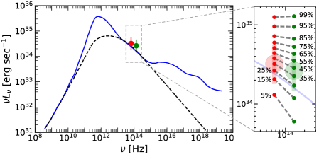
Figure 19: Observed and model spectral energy distributions for Sgr A*. Green and red points show, respectively, the 2.18 and 4.5 $\mu$m dim-phase luminosity densities of Sgr A*  as derived from the modes of the Case 3 analysis. The inset on the right shows several percentiles of the expected flux-density PDF as defined in Equation 13. The gray connection lines indicate the change of the $\nu L_{\nu}$ spectral slope $1-\alpha_{s}$ with luminosity. The blue line shows an SED model (Yuan et al., 2003) derived and normalized entirely from the radio part of the SED. The SED model assumes synchrotron radiation from electron populations with thermal and non-thermal energy distributions for the radio to NIR, and inverse Compton and bremsstrahlung emission for the higher frequencies. The black, dashed curve shows the non-thermal synchrotron model component (Yuan et al., 2003).

4.7 Black hole mass, luminosity, and rate of stochastic variability power

Meyer et al. (2009) found their Sgr A* break timescale consistent with mass–timescale relations of AGN in X-rays. However, it can be very difficult to obtain reliable break timescales from AGN light curves (Kelly et al., 2013). Kelly et al. analyzed X-ray and $0.51~{}\mu$m light curves of 39 AGN by introducing a parameter called “rate of stochastic variability power” (RSVP, designated $\xi^{2}$). This parameter is defined for damped random walks and quantifies the rate at which stochastic power driving the random walk is inserted. The RSVP is related to the total variance of the Ornstein-Uhlenbeck (OU) variability process (Kelly et al. 2009, 2013) by

$$\zeta^{2}=4\pi f_{b}\cdot{\rm Var}[F(t)]\quad.$$ (14)

For the 39 AGN observed by Kelly et al., $\zeta^{2}$ measured in X-rays correlates closely with black hole mass. While $\zeta^{2}$ as determined from visible light curves also scales with black hole mass, the (anti-)correlation with luminosity is even tighter.

As we have found here, Sgr A* is well described by an OU-process with a PSD slope of $\sim$2 with one break timescale (see also Meyer et al. 2014). Therefore we can use Equation 14 to derive $\zeta^{2}$ from the variance of the flux-density PDF and the break timescale. For Sgr A* at $M$, $\log{\zeta^{2}}=-2.61^{+0.16}_{-0.17}$. The value predicted by the empirical mass–RSVP relation (Kelly et al., 2013) is $\log{\zeta^{2}}\approx-7.4$, about five orders of magnitude smaller. This discrepancy might be expected because AGN are highly accreting objects, whereas Sgr A* has a tiny Eddington ratio. However, it is remarkable that the empirical luminosity–RSVP relation (Kelly et al., 2013) predicts $\log{\zeta^{2}}\approx-3.63$, close to the value for Sgr A*. Figure 20 compares Sgr A* with the Kelly et al. AGN, which have luminosities about nine orders of magnitude larger. While the uncertainties of the empirical relation put Sgr A* just outside the 1$\sigma$ envelope, the agreement is striking. These findings are even more surprising considering that the Kelly et al. (2013) interpretation for the luminosity–RSVP anti-correlation identifies the likely origin of the visible radiation as blackbody radiation from the outer parts of a thick accretion disk, whereas for Sgr A*, the NIR emission is non-thermal synchrotron radiation from the innermost accretion region.

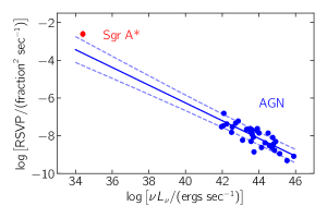
Figure 20: Rate of stochastic variability power (RSVP, §4.7) as a function of luminosity. Blue points denote 39 AGN observed by Kelly et al. (2013), and the solid line shows those authors’ Eq. 29. Dashed lines show the corresponding uncertainty envelope. The red point shows the RSVP for Sgr A* derived here.

4.8 Telescope photometric performance

While the observations from ground-based observatories do not include data after 2010 for the VLT and after 2013 for Keck (except the single 2016 data set), the VLT and Keck data used here constitute the most comprehensive and best characterized datasets available. They include most of the previously published $K$-band data for Sgr A*. In particular, they have been used in the statistical analyses of Witzel et al. (2012) and Meyer et al. (2014) and therefore provide a well understood baseline for the analysis of the 4.5 $\mu$m Spitzer data. Our analysis of the flux-density PDFs tells us which flux-density level in $M$-band corresponds to which level in $K$-band. This enables us to compare the relative sensitivity of each observatory to a given flux-density excursion. For a representative clock time of $\approx$1 minute (for which the Spitzer 8.4 s noise scales down by ${\approx}\sqrt{7}$ to $\sigma_{\rm{IRAC}}=0.05$ mJy) and large flux densities, the S/N proportions IRAC:NaCo:NIRC2 are 1:1.7:3.7. For low flux densities where $\Re({M}/{K})\approx 12$, S/N proportions become 2:1.7:3.7 (i.e., Spitzer/IRAC observing in $M$-band is competitive in S/N with ground-based AO imaging with 8–10 m-class telescopes observing in $K$). The future James Webb Space Telescope should be far superior at these wavelengths.

5 Conclusions

This paper has aimed to do the following:

• Presented the most comprehensive available set of NIR light curves of Sgr A*. Data were compiled from three observatories: the Spitzer Space Telescope, the ESO VLT, and the Keck observatory.

• Demonstrated the value of the new PSF extraction and fitting tool AIROPA on photometry for Sgr A*

• Introduced a new Bayesian method to determine the power spectral density of irregularly sampled, red-noise-dominated time series with non-Gaussian flux-density PDFs

• Determined the power spectral density and characteristic timescale $\tau_{b}=243^{+82}_{-57}$ minutes of the variability process with unprecedented precision

• Excluded PSD structure at timescales of 10–100 minutes. Such timescales correspond to the innermost stable circular orbit for black hole spin parameter $a<0.9$.

• Determined the spectral NIR properties of Sgr A* and the intrinsic flux-density PDFs with unprecedented accuracy. In particular, we confirmed the NIR spectral index of $\alpha_{s}\approx 0.6$ for flux densities above 0.3 mJy and found a redder spectral index at lower flux densities.

• Explored the spectral index dependence on flux density within the context of a electron energy distribution with exponential cutoff. We find the predicted submm levels and variability amplitudes to be consistent with the observed submm properties.

• Determined the dim phase SED in the NIR based on synchronous $K$- and $M$-band data, assuming a log-normal parametrization for the flux-density PDFs

• Demonstrated that Sgr A* is in agreement with the anti-correlation between luminosity and rate of stochastic variability power derived from visible light curves of more luminous AGN

• Showed that the Spitzer Space Telescope has relative photometric performance at $4.5~{}\mu$m on Sgr A* competitive with ground-based AO observations at $2.18~{}\mu$m

These results are especially of interest for the GRAVITY interferometric experiment at the Galactic Center. One of its goals is to measure the astrometric signature of hot spots moving close to the ISCO of the black hole. We expect that GRAVITY will not detect any such signature at timescales longer than 9 minutes as we do not find any NIR ISCO signature at these timescales. It seems imperative to design GRAVITY to operate at timescales significantly shorter than 10 minutes.

Another interesting result is the indication of the intrinsic turnover of the flux-density PDF at low flux-density levels in $M$-band. This means that $M$-band space-based observations are uniquely suited to explore all relevant timescales and the low flux-density regime, where the changes in timing and flux-density PDF possibly carry essential information about the physical processes at work. Sgr A* will be an essential target for the much more sensitive James Webb Space Telescope.

It is surprising how steady the statistical, spectral, and polarimetric parameters describing the variability of Sgr A* have been since the beginning of AO observations. The fact that the PSD parameters can be determined more precisely with a more extensive dataset and a better method implies that the PSD and PDF parameters are indeed self-consistent and nearly stationary over the last $\sim$15 years. (We have, however, not strictly tested stationarity in this analysis.) While one might expect the accretion process to be susceptible to abrupt changes in the supply of material (e.g., material stripped off G1 or G2), the NIR variability process shows no indication of that. The timescales at which matter travels from the typical periapsis distance of the G sources or S-stars ($>$100–200 au) are not clear. The interaction of infalling matter with the large number of fast-orbiting stars in the S-cluster might prevent larger clumps of gas from coherently finding their way to the innermost accretion region, thus regulating the steady supply of matter.

Appendix Appendix A Bayesian estimation of the flux-density ratio from synchronous data

Figure 4 shows simultaneous $K$ and $M$ light curves that match very closely. In order to derive the best flux-density ratio from these data, we modeled the $M$ flux-density as $F(M)=s\cdot F(K)+c$, where $s$ and $c$ are constants to be derived from the light curves. Each data point in the observed light curves can be modeled as

$$F_{i,\rm{real}}(M) \sim \mathcal{N}(s\cdot F_{i,\mathrm{real}}({K})+c,\sigma_{\mathrm{disp}}^{2})$$ (Appendix A1)

$$F_{i,\rm{obs}}(M) \sim \mathcal{N}(F_{i,\mathrm{real}}(M),\sigma_{M}^{2})$$ (Appendix A2)

$$F_{i,\rm{obs}}(K) \sim \mathcal{N}(F_{i,\mathrm{real}}(K),\sigma_{K}^{2})\quad,$$ (Appendix A3)

where $x\sim\mathcal{N}(\mu,\sigma^{2})$ denotes a normal distribution with mean $\mu$ and standard deviation $\sigma$. $F_{\mathrm{obs}}(M)$ and $F_{\mathrm{obs}}(K)$ are the observed flux densities including measurement white noise; $F_{\mathrm{real}}(M)$ and $F_{\mathrm{real}}(K)$ are idealized flux densities without measurement noise; $\sigma_{\rm{disp}}$ is an additional dispersion to allow the ideal ratio of $F_{\mathrm{real}}(M)$ and $F_{\mathrm{real}}(K)$ to differ as implied by the previously observed low-level and short-timescale spectral index fluctuations (Witzel et al., 2014). Integrating over the model parameters $F_{\mathrm{real}}(M)$ and $F_{\mathrm{real}}(K)$ gives

$$F_{i,\mathrm{obs}}(M)\sim\mathcal{N}(s\cdot F_{i,\mathrm{obs}}(K)+c,\sigma_{{M}}^{2}+s\cdot\sigma_{{K}}^{2}+\sigma_{\mathrm{disp}}^{2})\quad.$$ (Appendix A4)

We implemented this likelihood function with a MCMC Bayesian sampler in Pystan. With $\sigma_{{M}}=0.212$ (the $M$-band measurement noise for the rebinned IRAC data) and $\sigma_{{K}}=0.015$, we obtained the posteriors shown in Figure 5.

Appendix Appendix B Bayesian structure function analysis

For time series analyses of non-Gaussian-distributed light curves, there is generally no analytic expression for the likelihood function. That rules out a standard Bayesian approach, and instead we use a population Monte Carlo approximate Bayesian computation (PMC-ABC), which requires no prior knowledge of the likelihood function. The procedure was described by Ishida et al. (2015), but we have created our own C++ implementation tailored to the task of time series analysis. Our analysis procedure has four functional components:

• A method to randomly simulate data that mimic the observations as closely as possible. The method is based on a model parameterized by the quantities one wishes to determine. The model can be either statistical or deterministic or a combination.

• A distance function that quantifies how close the simulated data come to the available observations

• A prior distribution for each parameter

• The PMC-ABC sampler itself, which calls the three components above in the proper order

A previous approach to the PMC-ABC sampler was described by Ishida et al. (2015) and to data simulation by Witzel et al. (2012) and Hora et al. (2014). Notation and details for this work are explained below.

Appendix B.1 Simulating NIR light curves of Sgr A*

The power spectral density of the simulated data is a red-noise power-law spectrum with breaks at two frequencies, $f_{b}$ and $f_{b,2}$ (Fig. 21). The first break transitions between a slope $\gamma_{0}=0$ (for low frequencies corresponding to long time lags) to slope $\gamma_{1}$ and the second (at high frequencies corresponding to short time lags) from $\gamma_{1}$ to $\gamma_{2}$:

$$\mathrm{PSD}(f)\propto\left\{\begin{array}[]{lcl}f^{-\gamma_{0}}&\mathrm{for}&f<f_{b}\\ f^{-\gamma_{1}}&\mathrm{for}&f_{b}\leq f<f_{b,2}\\ f^{-\gamma_{2}}&\mathrm{for}&f\geq f_{b,2}\quad.\end{array}\right.$$ (Appendix B1)

For long time intervals $t\gg\tau_{b}\equiv 1/f_{b}$, the flux-density PDF (denoted $\mathcal{P}(F)$) is well described by a power law:

$$\mathcal{P}[F\mid(\beta,F_{0})]=\left\{\begin{array}[]{lll}\left[\frac{(\beta-1)}{-F_{0}}\right]\left[\frac{(F-F_{0})}{(-F_{0})}\right]^{-\beta}&\mathrm{for}&F\geq 0\quad,\\ 0&\mathrm{for}&F<0\quad,\end{array}\quad\right.$$ (Appendix B2)

where $\beta$ is the power law index and $F_{0}<0$ is the pole of the power-law. The cumulative distribution function is then

$${\rm{CDF}}[F\mid(\beta,F_{0})]\propto\bigg{(}\frac{F-F_{0}}{-F_{0}}\bigg{)}^{-\beta+1}\quad.$$ (Appendix B3)

An alternative distribution that describes the data in the observed range is a log-normal:

$$\mathcal{P}[F\mid(\mu_{\operatorname{logn}},\sigma_{\operatorname{logn}})]=\begin{array}[]{lcc}{{(\sqrt{2\pi}F\sigma_{\operatorname{logn}})}}^{-1}\cdot\exp{\left({-\frac{\left[{\ln{\left(\frac{F(K)}{\rm{mJy}}\right)}-\mu_{\operatorname{logn}}}\right]^{2}}{{\sqrt{2}\sigma_{\operatorname{logn}}^{2}}}}\right)}\quad,\end{array}$$ (Appendix B4)

with

$${\rm{CDF}}[F\mid(\mu_{\operatorname{logn}},\sigma_{\operatorname{logn}})]=\frac{1}{2}-\frac{1}{2}{\rm{erf}}\left[{\frac{\ln{\left(\frac{F(K)}{\rm{mJy}}\right)}-\mu_{\operatorname{logn}}}{\sqrt{2}\sigma_{\operatorname{logn}}}}\right]\quad,$$ (Appendix B5)

where $F\in[0,\inf]$, $\mu_{\operatorname{logn}}\in[-\inf,+\inf]$, and $\sigma_{\operatorname{logn}}\in[0,\inf]$.

To create light curves from the PSD in Eq. Appendix B1 that show the flux-density PDF of Equation Appendix B2, we used the Timmer & Koenig (1995) method as further developed by Witzel et al. (2012):

• Draw Fourier coefficients for each frequency from a Gaussian distribution with a variance proportional to the value of the PSD at that frequency.

• Fourier transform to the time domain giving normal-distributed random variable $y$, and normalize $y$ to unit variance.

• Sample $y$ to the cadence of the observed light curve.

• Transform $y$ into a power-law distributed random variable $T(y)$ that takes on values $0<T(y)<\infty$:

  $$T(y)=F_{{0}}-F_{{0}}\cdot\left\{\frac{1}{2}\left[1+{\mathrm{erf}}\left(\frac{y}{\sqrt{2}}\right)\right]\right\}^{{\left(1-\beta\right)}^{-1}}\quad,$$ (Appendix B6)

  where ‘erf’ is the Gaussian error function, $\beta$ is the power-law index, and $F_{0}$ is the power-law pole of Equation Appendix B2. For the alternative log-normal distribution, use instead

  $$T(y)=\exp{\big{(}\sigma_{\operatorname{logn}}\cdot y+\mu_{\operatorname{logn}}\big{)}}\quad.$$ (Appendix B7)

• Draw Gaussian noise (independent for each point), and add it to each point to account for the measurement errors.

The above method allows generating light curves according to any calibrated PSD of the form of Eq. Appendix B1 – that is, distributed as the observed data on all timescales. In particular, it enables comparison of the absolute values of the structure functions of simulated light curves with the observed structure function. The transformation of Equation Appendix B6 or Appendix B7 changes the PSD of the generated light curve slightly (Figure 21), but the break timescales are invariant under this transformation.

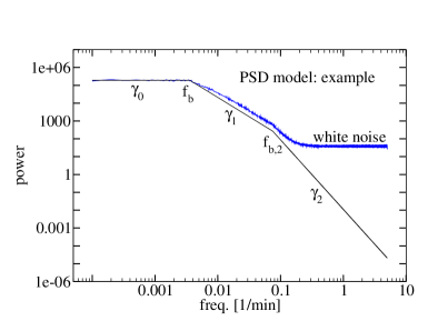
Figure 21: The PSD model before and after nonlinear transformation. The black lines show an example PSD model with two break timescales. Because the abscissa is in frequency space, short timescales are to the right. In the notation used here, the first break frequency at ${\sim}3\times 10^{-3}$ minutes^-1 is $f_{b}$, and the second break frequency at $\sim$0.1 minutes^-1 is $f_{b,2}$. Slopes of the three segments are from left to right $\gamma_{0}=0$, $\gamma_{1}$, and $\gamma_{2}$. The last is indeterminate in the actual data, because no second break can be found. The blue curves show a simulated measurement of the example PSD (Appendix B.1) based on an average FFT periodogram of 1000 equally sampled light curves with 6 s cadence and a duration of $10^{4}$ minutes.

Appendix B.2 The distance function

The distance function $\phi$ quantifies the difference between two data sets. This function is used in the PMC-ABC algorithm to compare randomly drawn mock data sets to the measured data (see section Appendix B.4 below). We based our distance function on the first-order structure function defined by

$$V(\tau_{i})=\frac{1}{n_{i}}\sum_{t_{j},t_{k}}\left[F(t_{j})-F(t_{k})\right]^{2}\quad\mathrm{for}\quad\tau_{i}\leq(t_{j}-t_{k})<\tau_{i+1}\quad,$$ (Appendix B8)

that is, the sum of $\left[F(t_{j})-F(t_{k})\right]$ over all $n_{i}$ existing pairs whose time lags $(t_{j}-t_{k})$ fall within the bin $[\tau_{i},\tau_{i+1}]$. We defined the distance between two light curves as the weighted L2 norm of the difference between the logarithms of the respective structure function’s binned values:

$$\phi(V_{1},V_{2})=\sum_{i}w_{i}(\log\left[V_{1}(\tau_{i})/V_{2}(\tau_{i})\right])^{2}\quad$$ (Appendix B9)

with $w_{i}$ the weights for the chosen binning. These weights control the relative influence of each data set on the results, not the accuracy to which the structure function is approximated. For a sufficient number of iterations, any weighting scheme converges to the same result. The relative weights unity for each structure function bin, except for the single wide bin at large time lags (see §3 ), which had a weight of 3. Additionally, we weighted the structure function from the NIRC2 data with 0.67 relative to the IRAC and NaCo data

Appendix B.3 Prior distributions

We used a combination of flat and Gaussian priors. The latter are appropriate for the few cases of independently well-determined parameters such as the measurement noise. In order to guarantee a monotonically decreasing function for the PSD, we applied the conditions

$$f_{b,2}>f_{b}~{}~{}\mathrm{and}~{}~{}\gamma_{2}>\gamma_{1}$$ (Appendix B10)

to the flat joint prior distributions for the PSD, $\mathcal{P}(\gamma_{1},\gamma_{2})$ and $\mathcal{P}(f_{b},f_{b,2})$. While the joint prior distributions of $\gamma_{1}$, $\gamma_{2}$, $f_{b}$, and $f_{b,2}$ are uniform, their marginalized distributions are not because of the conditions in Eq. Appendix B10. In this case, the cumulative distribution functions of the marginalized probabilities are quadratic in their respective parameters. Therefore drawing from a joint uniform probability distribution subject to the constraints in Eq. Appendix B10 can be obtained by

$$f_{b} = f_{max}-(f_{max}-f_{min})\cdot\sqrt{\mathfrak{u}_{f,1}}$$ (Appendix B11)

$$f_{b,2} = (f_{max,2}-f_{b})\cdot\mathfrak{u}_{f,2}+f_{b}$$ (Appendix B12)

and

$$\gamma_{1} = \gamma_{max}-(\gamma_{max}-\gamma_{min})\cdot\sqrt{\mathfrak{u}_{\gamma,1}}$$ (Appendix B13)

$$\gamma_{2} = (\gamma_{max,2}-\gamma_{1})\cdot\mathfrak{u}_{\gamma,2}+\gamma_{1}$$ (Appendix B14)

where $\mathfrak{u}_{f,i}$ and $\mathfrak{u}_{\gamma,i}$ are random variables uniformly distributed on $[0,1]$.

Appendix B.4 The PMC-ABC sampler

Approximate Bayesian Computation (ABC) is a useful computational algorithm for Bayesian parameter space exploration where explicit likelihood evaluations are either impossible or not feasible (Cameron & Pettitt, 2012; Marjoram et al., 2003; Sisson et al., 2007). The goal is to estimate the posterior by finding a set of mock light curves ($\sim$10,000 in our case) that agree with the actual data within specified limits. The input parameter sets from which these light curves were generated provide an approximation of the source parameters’ posterior if these variability parameters were drawn from distributions that are statistically consistent with the priors. In principle, one could simply draw from the prior as often as it takes to find 10,000 accepted light curves. However, this approach becomes computationally impossible for tight limits. Instead, the PMC-ABC algorithm implemented here is iterative and informed by the posterior estimate of the previous iteration, focusing its search on regions of parameter space in which acceptable light curves are most likely to be found.

At its core, the basic ABC algorithm consists of two Monte Carlo sampling steps and an acceptance step. Each iteration starts by selecting a random model parameter set $\mathscr{\theta}$ from a predefined probability distribution $\mathcal{P}(\mathscr{\theta})$. Given the parameter set, a random mock data set $\widetilde{\mathscr{D}}$ is drawn from the likelihood $\mathcal{P}(\widetilde{\mathscr{D}}\mid\mathscr{\theta})$. This mock data set is compared to the actual data set through the distance function $\phi({\mathscr{D}},\widetilde{\mathscr{D}})$. If ($|\phi({\mathscr{D}},\widetilde{\mathscr{D}})|<\epsilon$), where $\epsilon$ is a chosen limit, the drawn parameter set is accepted. These steps repeat until enough mock data sets are accepted.

The ABC algorithm explores the approximate posterior probability distribution:

$$\widetilde{\mathcal{P}}(\mathscr{\theta}\mid\mathscr{D})\equiv\mathcal{P}(\mathscr{\theta}\mid|\phi({\mathscr{D}},\widetilde{\mathscr{D}})|<\epsilon)\propto\int\mathcal{W}(\phi(\mathscr{D},\widetilde{\mathscr{D}})\mid\epsilon)\mathcal{P}(\widetilde{\mathscr{D}}\mid\mathscr{\theta})\mathcal{P}(\mathscr{\theta})\ d\widetilde{\mathscr{D}}\quad,$$ (Appendix B15)

where $\mathcal{W}(\cdot\mid\epsilon)$ is a top-hat window function with width $\epsilon$. Given an adequate distance function, the approximate posterior becomes exact as $\epsilon\rightarrow 0$, but the chance of accepting a drawn parameter set becomes vanishingly small. Therefore, as mentioned, a naive application of the ABC algorithm would be computationally infeasible. The PMC-ABC algorithm is a variant of the normal ABC algorithm that attempts to improve ABC performance by iteratively applying a population Monte Carlo technique to “learn” the important regions of parameter space (Ishida et al., 2015; Drovandi & Pettitt, 2011). The PMC-ABC algorithm iteratively modifies a population of parameter combinations (a “particle system” $\mathscr{C}$) and a list of weights corresponding to each parameter combination. With each iteration, the weighted particle system asymptotically approaches the target posterior distribution. Each iteration’s parameter combinations are drawn from a distribution $\overline{\mathcal{P}}(\mathscr{\theta})$ inferred from the previous iteration’s particle system. In our implementation, we smooth over the previous iteration’s particle system using a Gaussian kernel whose dispersion is the dispersion of the previous particle system ($\{\theta_{n-1,i}\}$), thereby selecting from a distribution of

$$\overline{\mathcal{P}}(\theta)\propto\sum_{i}\mathcal{K}(\theta\mid\theta_{n-1,i},\Sigma)$$ (Appendix B16)

where $\mathcal{K}(\cdot\mid\cdot,\Sigma)$ is a Gaussian kernel with dispersion $\Sigma$. $\overline{\mathcal{P}}(\theta)$ is truncated to be within the prior range. The mock data set is then drawn, and the resulting parameter combination is accepted if the distance from the real data is below $\epsilon$. $\epsilon$ is decreased for each iteration by selecting the 45th percentile largest distance value from the previous iteration’s accepted parameter sets. Because the parameter values at stages after the first are not selected from the prior but from a “proposal distribution” based on the previous posterior estimate, the resultant parameter points must be reweighted by a factor $\mathcal{P}(\mathscr{\theta})/\overline{\mathcal{P}}(\mathscr{\theta})$. This reweighting makes the proposal distribution statistically consistent with the prior. The algorithm is iterated until the acceptance ratio decreases to a user-specified value. The diagram Algorithm 1 summarizes the required steps.

while size of $\mathscr{C}_{\rm{start}}<M$ do

       Draw $\mathscr{\theta}$, from the prior, $\mathcal{P}(\mathscr{\theta})$.

       Use $\mathscr{\theta}$ to generate $\widetilde{\mathscr{D}}$.

       Save $\mathscr{\theta}$ as part of next generation particle system, $\mathscr{C}_{\rm{start}}$.

end while

Save N points in $\mathscr{C}_{\rm{start}}$ with the lowest distance values to $\mathscr{C}$.

Set weights to $1/N$

while Acceptance ratio is above $\alpha$ do

       Infer $\overline{\mathcal{P}}(\mathscr{\theta})$ from $\mathscr{C}$.

       Set $\epsilon$ to the 45% quantile of the ordered distances in $\mathscr{C}$.

       while size of $\mathscr{C}_{\rm{next}}<N$ do

             Draw $\mathscr{\theta}$ from $\overline{\mathcal{P}}(\mathscr{\theta})$.

             Use $\mathscr{\theta}$ to generate $\widetilde{\mathscr{D}}$.

             if $|\phi(\widetilde{\mathscr{D}},\mathscr{D})|<\epsilon$ then

                   Save $\mathscr{\theta}$ as part of next generation particle system, $\mathscr{C}_{\rm{next}}$.

                   Set weight to $\mathcal{P}(\mathscr{\theta})/\overline{\mathcal{P}}(\mathscr{\theta})$

             end if

            

       end while

      $\mathscr{C}\leftarrow\mathscr{C}_{\rm{next}}$

end while

Algorithm 1 PMC-ABC algorithm.

Appendix Appendix C Efficient calculation of the first-order structure function

The time-series analysis technique used here requires multiple structure function calculations that share identical observing cadences. This can be resource-intensive because the number of operations needed to calculate each structure function (Eq. Appendix B8) is proportional to the square of the number $N$ of light curve data points. Direct calculation made this step the primary computational bottleneck. To reduce computation time, we developed a more efficient algorithm for calculating structure functions that share identical observing cadences. Central to our algorithm is the comparison of a “perfect” structure function defined by

$$\widetilde{V}_{i} = \frac{1}{N}\sum_{k=0}^{N-i-1}(F(t_{k+i})-F(t_{k}))^{2}$$ (Appendix C1)

$$= \frac{1}{N}\sum_{k=0}^{N-i-1}(F(t_{k+i})^{2}+F(t_{k})^{2})-\frac{2}{N}\sum_{k=0}^{N-i-1}F(t_{k+i})F(t_{k})$$ (Appendix C2)

$$= \widetilde{\Phi}_{i}^{0}+2\widetilde{\Phi}_{i}^{1}~{}.$$ (Appendix C3)

to the actual structure function calculated from Eq. Appendix B8, which needs to be evaluated only once. This is advantageous because the number of operations for the second term $\widetilde{\Phi}_{i}^{1}$ of Eq. Appendix C3 goes as $N\log N$ when calculated via fast Fourier transforms. The first term $\widetilde{\Phi}_{i}^{0}$ can be calculated recursively ($\widetilde{\Phi}_{i}^{0}=\widetilde{\Phi}_{i+1}^{0}+F(t_{N-1-i})^{2}+F(t_{i})^{2};\widetilde{\Phi}_{N}^{0}=0$), which is linear in $N$. Replacing flux pairs in the actual binned structure function (Eq. Appendix B8) with the corresponding perfect structure function values therefore shortens computation time. Unfortunately, some perfect structure function values will be shared between multiple bins, and these values will need to be split between these bins. In such cases, light curve pairs must be explicitly calculated and added to or subtracted from the affected bins. In practice, for observing cadences that are fairly even, few light curve pairs need to be calculated directly, and these have negligible effect on computational performance. For observing cadences that are very uneven, up to 30% of the light curve pairs require direct calculation. Even in such cases, though, the above algorithm still offers significant performance improvements for multiple structure function calculations that share the same observing cadence.

Appendix Appendix D Ratio between $M$- and $K$-band derived from power-law and log-normal distributions

Any model that allows different flux-density PDFs for $M$- and $K$-band predicts a varying $F(M)/F(K)$ ratio as a function of $F(K)$. This is true even when both distributions are power laws if the power-law index $\beta$ differs for the two bands. A simple way to calculate the ratio function – that is, the ratio $\Re[M/K,F(K)]\equiv F(M)/F(K)$ as a function of $F(K)$ – is the assumption that the cumulative distribution functions (as defined in Eq. Appendix B3 or Appendix B5) are equal for all corresponding pairs $[F(K),(F(M)]$. This is simply asking for a match of the lowest $5\%$ in $K$-band with the lowest $5\%$ in $M$-band, the lowest $10\%$ with the lowest $10\%$, and so on. In other words, it assumes that when $K$-band rises, $M$-band rises, and when $K$-band falls, $M$-band falls. The simultaneous NIR (1.65–3.8 µm) light curves in the literature indeed demonstrate this behavior. Under this assumption, we get for Case 1 (power-law/power-law):

$$\Re[M/K,F(K)]=\frac{s\cdot F_{0}(M)}{F(K)}\bigg{\{}1-\bigg{[}\frac{F(K)-F_{0}(K)}{-F_{0}(K)}\bigg{]}^{\frac{\beta_{{K}}-1}{\beta_{{M}}-1}}\bigg{\}}\quad,$$ (Appendix D1)

with $F_{0,{M}},F_{0,{K}}<0$. For Case 2 (power-law/log-normal),

$$\Re[M/K,F(K)]=\bigg{[}\frac{F(K)}{\rm{mJy}}\bigg{]}^{-1}\cdot\exp{\bigg{[}{\mu_{\operatorname{logn,M}}\sqrt{2}\sigma_{\operatorname{logn,M}}\cdot\mathrm{erf}^{-1}\big{(}1-2\kappa\big{)}}\bigg{]}}\quad,$$ (Appendix D2)

with

$$\kappa=\bigg{(}\frac{F_{{K}}-F_{0,{K}}}{-F_{0,{K}}}\bigg{)}^{1-\beta_{{K}}}\quad,$$ (Appendix D3)

and with $F_{0,{K}}<0$. For Case 3 (log-normal/log-normal),

$$\Re[M/K,F(K)]=\left[\frac{F(K)}{\rm{mJy}}\right]^{-1}\cdot\exp{\left\{\left(\ln{\left[\frac{F(K)}{\rm{mJy}}\right]}-\mu_{\operatorname{logn},K}\right)\cdot\frac{\sigma_{\operatorname{logn},M}}{\sigma_{\operatorname{logn},K}}+\mu_{\operatorname{logn},M}\right\}}\quad.$$ (Appendix D4)

In order to use the information about the flux-density ratio determined from the synchronous data ($\Re[M/K,0.15~{}{\rm mJy}]=12.4\pm 0.5$), we can use this equation and extend the Equation Appendix B9 distance function to

$$\phi(\theta)=\phi(V_{\theta},V_{\rm{obs.}})+w\cdot\bigg{\{}\big{[}X-\Re(M/K,0.15)\big{]}/0.5\bigg{\}}^{2}\quad,$$ (Appendix D5)

with $X\sim\mathcal{N}(12.4,0.5^{2})$ and $w$ a chosen weight. (Here, $w=0.002$ relative to the weights defined in Appendix B.2.) The corresponding NIR spectral index

$$\alpha_{s}=\left\{{\log{\big{(}\frac{\lambda_{M}}{\lambda_{K}}\big{)}}}\right\}^{-1}\cdot\bigg{\{}\log{\big{[}\Re(M/K)\big{]}}+0.4\cdot(A_{M}-A_{K})\bigg{\}}\quad,$$ (Appendix D6)

where $A_{M}$ and $A_{K}$ are the adopted interstellar extinctions in magnitudes. For our case with

$$\log\big{\{}\Re[M/K,F(K)]\big{\}}=\bigg{(}\frac{\sigma_{\operatorname{logn},M}}{\sigma_{\operatorname{logn},K}}-1\bigg{)}\cdot\log{\bigg{[}\frac{F(K)}{\rm{mJy}}\bigg{]}}+0.4343\cdot\bigg{(}\mu_{\operatorname{logn},M}-\frac{\sigma_{\operatorname{logn},M}}{\sigma_{\operatorname{logn},K}}\cdot\mu_{\operatorname{logn},K}\bigg{)}$$ (Appendix D7)

and with $\lambda_{M}=4.5$ µm and $\lambda_{K}=2.18$ µm,

$$\alpha_{s} = 3.1771\cdot\bigg{(}\frac{\sigma_{\operatorname{logn},M}}{\sigma_{\operatorname{logn},K}}-1\bigg{)}\cdot\log{\bigg{[}\frac{F(K)}{\rm{mJy}}\bigg{]}}+1.3798\cdot\bigg{(}\mu_{\operatorname{logn},M}-\frac{\sigma_{\operatorname{logn},M}}{\sigma_{\operatorname{logn},K}}\cdot\mu_{\operatorname{logn},K}\bigg{)}+1.2708\cdot(A_{M}-A_{K})$$ (Appendix D8)

$$= \xi\cdot\log{\bigg{[}\frac{F(K)}{\rm{mJy}}\bigg{]}}+\eta+1.2708\cdot(A_{M}-A_{K})\quad.$$ (Appendix D9)

Appendix Appendix E NIR spectral index as a function of flux density

For synchrotron radiation from an electron energy distribution with an exponential cutoff, the spectrum in the optically thin frequency regime is a power-law with an exponential cutoff at a frequency $\nu_{0}$ (e.g., Bregman 1985). The flux density $S(\nu)$ at a given frequency $\nu$ in the optically thin regime is

$$S(\nu)=k_{0}\cdot\nu^{-\tilde{\alpha}_{s}}\cdot\exp{\big{[}-\big{(}{\nu}/{\nu_{0}}\big{)}^{{1}/{2}}\big{]}}\quad,$$ (Appendix E1)

with $\tilde{\alpha}_{s}$ the spectral index of the optically thin power-law spectrum . For typical electron energy cutoffs, $\nu_{0}$ will be located in or slightly above the NIR frequency range. Thus varying flux densities in the NIR and a flux-density-dependent NIR spectral index could be the consequence of a changing energy cutoff in the electron energy distribution.

We want to derive the flux-density dependence of the spectral index for this scenario. For a frequency $\tilde{\nu}\ll\nu_{0}$ (but still in the optically thin regime; i.e., in the submm regime close to 1 THz), Equation Appendix E1 becomes

$$S(\tilde{\nu})=k_{0}\cdot\tilde{\nu}^{-\tilde{\alpha}_{s}}\quad,$$ (Appendix E2)

and we can eliminate the proportionality factor:

$$S(\nu)=S(\tilde{\nu})\cdot\big{(}{\nu}/{\tilde{\nu}}\big{)}^{-\tilde{\alpha}_{s}}\cdot\exp{\big{[}-\big{(}{\nu}/{\nu_{0}}\big{)}^{{1}/{2}}\big{]}}\quad.$$ (Appendix E3)

This equation implies that while the flux density in the NIR overall scales with flux density in the submm, for a given submm flux density the NIR variability is caused by the changes in $\nu_{0}$. The flux-density ratio between two frequencies $\nu_{1}$ and $\nu_{2}$ is

$${S(\nu_{1})}/{S(\nu_{2})} = \big{(}{\nu_{1}}/{\nu_{2}}\big{)}^{-\tilde{\alpha}_{s}}\cdot\exp{\big{[}\big{(}{\nu_{2}}/{\nu_{0}}\big{)}^{{1}/{2}}-\big{(}{\nu_{1}}/{\nu_{0}}\big{)}^{{1}/{2}}\big{]}}\quad,$$ (Appendix E4)

and

$$\alpha_{s}=\tilde{\alpha}_{s}-{\nu_{0}^{-{1}/{2}}}\cdot\frac{\nu_{2}^{\nicefrac{{1}}{{2}}}-\nu_{1}^{\nicefrac{{1}}{{2}}}}{\ln{(10)}\cdot\log{\big{(}{\nu_{1}}/{\nu_{2}}\big{)}}}\quad.$$ (Appendix E5)

Equation Appendix E3 gives

$${\nu_{0}^{-\nicefrac{{1}}{{2}}}} = {-\nu^{-{1}/{2}}}\cdot{\ln{(10)}}\cdot\left\{\log{\left[{S(\nu)}/{S(\tilde{\nu})}\right]}+\tilde{\alpha}_{s}\cdot\log{\left({\nu}/{\tilde{\nu}}\right)}\right\}~{}~{}\rm{with}$$ (Appendix E6)

$$S(\tilde{\nu}) < 10^{\tilde{\alpha}_{s}\cdot\log{(\nicefrac{{\nu}}{{\tilde{\nu}}})}}\cdot S(\nu)\quad.$$ (Appendix E7)

Inserting Equation Appendix E6 in Equation Appendix E5 gives

$$\alpha_{s} = \tilde{\xi}\cdot\log{\left[\frac{S(\nu)}{\rm{mJy}}\right]}+\tilde{\eta}\quad,$$ (Appendix E8)

with

$$\tilde{\xi}=\frac{\nu_{2}^{\nicefrac{{1}}{{2}}}-\nu_{1}^{\nicefrac{{1}}{{2}}}}{\nu^{\nicefrac{{1}}{{2}}}\cdot\log{\big{(}{\nu_{1}}/{\nu_{2}}\big{)}}}$$ (Appendix E9)

and

$$\tilde{\eta}=\tilde{\alpha}_{s}\cdot\left[1+\tilde{\xi}\cdot\log{\left({\nu}/{\tilde{\nu}}\right)}\right]-\tilde{\xi}\cdot\log{\left[\frac{S(\tilde{\nu})}{\rm{mJy}}\right]}\quad.$$ (Appendix E10)

References

- Akeret et al. (2015) Akeret, J., Refregier, A., Amara, A., Seehars, S., & Hasner, C. 2015, J. Cosmology Astropart. Phys, 8, 043
- Astropy Collaboration: Robitaille et al. (2013) Astropy Collaboration: Robitaille, T. P., Tollerud, E. J., Greenfield, P., et al. 2013, A&A, 558, A33
- Baganoff et al. (2001) Baganoff, F. K., Bautz, M. W., Brandt, W. N., et al. 2001, Nature, 413, 45
- Balick & Brown (1974) Balick, B., & Brown, R. L. 1974, ApJ, 194, 265
- Bardeen et al. (1972) Bardeen, J. M., Press, W. H., & Teukolsky, S. A. 1972, ApJ, 178, 347
- Boehle et al. (2016) Boehle, A., Ghez, A. M., Schödel, R., et al. 2016, ApJ, 830, 17
- Bower et al. (2015) Bower, G. C., Markoff, S., Dexter, J., et al. 2015, ApJ, 802, 69
- Bregman (1985) Bregman, J. N. 1985, ApJ, 288, 32
- Bremer et al. (2011) Bremer, M., Witzel, G., Eckart, A., et al. 2011, A&A, 532, A26
- Cameron & Pettitt (2012) Cameron, E., & Pettitt, A. N. 2012, MNRAS, 425, 44
- Capellupo et al. (2017) Capellupo, D. M., Haggard, D., Choux, N., et al. 2017, ApJ, 845, 35
- Carpenter et al. (2017) Carpenter, B., Gelman, A., D. Hoffman, M., et al. 2017, Journal of Statistical Software, 76, 1
- Dexter et al. (2014) Dexter, J., Kelly, B., Bower, G. C., et al. 2014, MNRAS, 442, 2797
- Dibi et al. (2016) Dibi, S., Markoff, S., Belmont, R., et al. 2016, MNRAS, 461, 552
- Diolaiti et al. (2000) Diolaiti, E., Bendinelli, O., Bonaccini, D., et al. 2000, in Proc. SPIE, Vol. 4007, 879–888
- Do et al. (2009) Do, T., Ghez, A. M., Morris, M. R., et al. 2009, ApJ, 691, 1021
- Do et al. (2013) Do, T., Lu, J. R., Ghez, A. M., et al. 2013, ApJ, 764, 154
- Dodds-Eden et al. (2010) Dodds-Eden, K., Sharma, P., Quataert, E., et al. 2010, ApJ, 725, 450
- Dodds-Eden et al. (2009) Dodds-Eden, K., Porquet, D., Trap, G., et al. 2009, ApJ, 698, 676
- Dodds-Eden et al. (2011) Dodds-Eden, K., Gillessen, S., Fritz, T. K., et al. 2011, ApJ, 728, 37
- Dolence et al. (2012) Dolence, J. C., Gammie, C. F., Shiokawa, H., & Noble, S. C. 2012, ApJ, 746, L10
- Drovandi & Pettitt (2011) Drovandi, C. C., & Pettitt, A. N. 2011, Biometrics, 67, 225
- Eckart et al. (2006a) Eckart, A., Schödel, R., Meyer, L., et al. 2006a, A&A, 455, 1
- Eckart et al. (2004) Eckart, A., Baganoff, F. K., Morris, M., et al. 2004, A&A, 427, 1
- Eckart et al. (2006b) Eckart, A., Baganoff, F. K., Schödel, R., et al. 2006b, A&A, 450, 535
- Eckart et al. (2008a) Eckart, A., Baganoff, F. K., Zamaninasab, M., et al. 2008a, A&A, 479, 625
- Eckart et al. (2008b) Eckart, A., Schödel, R., García-Marín, M., et al. 2008b, A&A, 492, 337
- Eckart et al. (2009) Eckart, A., Baganoff, F. K., Morris, M. R., et al. 2009, A&A, 500, 935
- Eckart et al. (2012) Eckart, A., García-Marín, M., Vogel, S. N., et al. 2012, A&A, 537, A52
- Eisenhauer et al. (2005) Eisenhauer, F., Genzel, R., Alexander, T., et al. 2005, ApJ, 628, 246
- Emmanoulopoulos et al. (2010) Emmanoulopoulos, D., McHardy, I. M., & Uttley, P. 2010, MNRAS, 404, 931
- Falcke et al. (1998) Falcke, H., Goss, W. M., Matsuo, H., et al. 1998, ApJ, 499, 731
- Falcke & Markoff (2000) Falcke, H., & Markoff, S. 2000, A&A, 362, 113
- Fazio et al. (2018) Fazio, G. G., Marrone, D., Hora, J. L., et al. 2018, ApJ, accepted, arXiv:1807.07599
- Foreman-Mackey (2016) Foreman-Mackey, D. 2016, The Journal of Open Source Software, 24, 1
- Frigo & Johnson (2005) Frigo, M., & Johnson, S. G. 2005, Proceedings of the IEEE, 93, 216, special issue on “Program Generation, Optimization, and Platform Adaptation”
- Gandhi (2009) Gandhi, P. 2009, The Astrophysical Journal Letters, 697, L167
- García-Marín et al. (2011) García-Marín, M., Eckart, A., Weiss, A., et al. 2011, ApJ, 738, 158
- Genzel et al. (2003) Genzel, R., Schödel, R., Ott, T., et al. 2003, Nature, 425, 934
- Ghez et al. (2005a) Ghez, A. M., Salim, S., Hornstein, S. D., et al. 2005a, ApJ, 620, 744
- Ghez et al. (2004) Ghez, A. M., Wright, S. A., Matthews, K., et al. 2004, ApJ, 601, L159
- Ghez et al. (2005b) Ghez, A. M., Hornstein, S. D., Lu, J. R., et al. 2005b, ApJ, 635, 1087
- Gillessen et al. (2006) Gillessen, S., Eisenhauer, F., Quataert, E., et al. 2006, ApJ, 640, L163
- Guan et al. (2009) Guan, X., Gammie, C. F., Simon, J. B., & Johnson, B. M. 2009, ApJ, 694, 1010
- Haubois et al. (2012) Haubois, X., Dodds-Eden, K., Weiss, A., et al. 2012, A&A, 540, A41
- Herrnstein et al. (2004) Herrnstein, R. M., Zhao, J.-H., Bower, G. C., & Goss, W. M. 2004, AJ, 127, 3399
- Hora et al. (2014) Hora, J. L., Witzel, G., Ashby, M. L. N., et al. 2014, ApJ, 793, 120
- Hornstein et al. (2002) Hornstein, S. D., Ghez, A. M., Tanner, A., et al. 2002, ApJ, 577, L9
- Hornstein et al. (2007) Hornstein, S. D., Matthews, K., Ghez, A. M., et al. 2007, ApJ, 667, 900
- Hughes et al. (1992) Hughes, P. A., Aller, H. D., & Aller, M. F. 1992, ApJ, 396, 469
- Hunter (2007) Hunter, J. D. 2007, Computing in Science Engineering, 9, 90
- Ishida et al. (2015) Ishida, E. E. O., Vitenti, S. D. P., Penna-Lima, M., et al. 2015, Astronomy and Computing, 13, 1
- Jones et al. (2001) Jones, E., Oliphant, T., Peterson, P., et al. 2001, SciPy: Open source scientific tools for Python, [http://www.scipy.org/; accessed 2018 April 1]
- Karssen et al. (2017) Karssen, G. D., Bursa, M., Eckart, A., et al. 2017, MNRAS, 472, 4422
- Kelly et al. (2009) Kelly, B. C., Bechtold, J., & Siemiginowska, A. 2009, ApJ, 698, 895
- Kelly et al. (2013) Kelly, B. C., Treu, T., Malkan, M., Pancoast, A., & Woo, J.-H. 2013, ApJ, 779, 187
- Kozłowski (2016) Kozłowski, S. 2016, ApJ, 826, 118
- Krabbe et al. (2006) Krabbe, A., Iserlohe, C., Larkin, J. E., et al. 2006, ApJ, 642, L145
- Kunneriath et al. (2010) Kunneriath, D., Witzel, G., Eckart, A., et al. 2010, A&A, 517, A46
- Lenzen et al. (2003) Lenzen, R., Hartung, M., Brandner, W., et al. 2003, in Presented at the Society of Photo-Optical Instrumentation Engineers (SPIE) Conference, Vol. 4841, Society of Photo-Optical Instrumentation Engineers (SPIE) Conference Series, ed. M. Iye & A. F. M. Moorwood, 944–952
- Li et al. (2009) Li, J., Shen, Z.-Q., Miyazaki, A., et al. 2009, ApJ, 700, 417
- Mahadevan (1998) Mahadevan, R. 1998, Nature, 394, 651
- Marjoram et al. (2003) Marjoram, P., Molitor, J., Plagnol, V., & Tavaré, S. 2003, Proceedings of the National Academy of Science, 100, 15324
- Marrone et al. (2006) Marrone, D. P., Moran, J. M., Zhao, J.-H., & Rao, R. 2006, ApJ, 640, 308
- Marrone et al. (2007) —. 2007, ApJ, 654, L57
- Marrone et al. (2008) Marrone, D. P., Baganoff, F. K., Morris, M. R., et al. 2008, ApJ, 682, 373
- Mauerhan et al. (2005) Mauerhan, J. C., Morris, M., Walter, F., & Baganoff, F. K. 2005, ApJ, 623, L25
- McHardy et al. (2006) McHardy, I. M., Koerding, E., Knigge, C., Uttley, P., & Fender, R. P. 2006, Nature, 444, 730
- Melia & Falcke (2001) Melia, F., & Falcke, H. 2001, ARA&A, 39, 309
- Meyer et al. (2008) Meyer, L., Do, T., Ghez, A., et al. 2008, ApJ, 688, L17
- Meyer et al. (2009) —. 2009, ApJ, 694, L87
- Meyer et al. (2006a) Meyer, L., Eckart, A., Schödel, R., et al. 2006a, A&A, 460, 15
- Meyer et al. (2007) Meyer, L., Schödel, R., Eckart, A., et al. 2007, A&A, 473, 707
- Meyer et al. (2006b) —. 2006b, A&A, 458, L25
- Meyer et al. (2014) Meyer, L., Witzel, G., Longstaff, F. A., & Ghez, A. M. 2014, ApJ, 791, 24
- Miyazaki et al. (2004) Miyazaki, A., Tsutsumi, T., & Tsuboi, M. 2004, ApJ, 611, L97
- Moffet (1975) Moffet, A. T. 1975, Strong Nonthermal Radio Emission from Galaxies, ed. A. Sandage, M. Sandage, & J. Kristian (the University of Chicago Press), 211
- Morris et al. (2012) Morris, M. R., Meyer, L., & Ghez, A. M. 2012, Research in Astronomy and Astrophysics, 12, 995
- Mossoux et al. (2016) Mossoux, E., Grosso, N., Bushouse, H., et al. 2016, A&A, 589, A116
- Neilsen et al. (2013) Neilsen, J., Nowak, M. A., Gammie, C., et al. 2013, ApJ, 774, 42
- Neilsen et al. (2015) Neilsen, J., Markoff, S., Nowak, M. A., et al. 2015, ApJ, 799, 199
- Nishiyama et al. (2009) Nishiyama, S., Tamura, M., Hatano, H., et al. 2009, ApJ, 702, L56
- Özel et al. (2000) Özel, F., Psaltis, D., & Narayan, R. 2000, ApJ, 541, 234
- Ponti et al. (2017) Ponti, G., George, E., Scaringi, S., et al. 2017, MNRAS, 468, 2447
- Porquet et al. (2008) Porquet, D., Grosso, N., Predehl, P., et al. 2008, A&A, 488, 549
- Rauch et al. (2016) Rauch, C., Ros, E., Krichbaum, T. P., et al. 2016, A&A, 587, A37
- Sabha et al. (2010) Sabha, N., Witzel, G., Eckart, A., et al. 2010, A&A, 512, A2
- Sabha et al. (2012) Sabha, N., Eckart, A., Merritt, D., et al. 2012, A&A, 545, A70
- Schödel et al. (2011) Schödel, R., Morris, M. R., Muzic, K., et al. 2011, A&A, 532, A83
- Schödel et al. (2010) Schödel, R., Najarro, F., Muzic, K., & Eckart, A. 2010, A&A, 511, A18
- Shahzamanian et al. (2015) Shahzamanian, B., Eckart, A., Valencia-S., M., et al. 2015, A&A, 576, A20
- Sharma et al. (2007) Sharma, P., Quataert, E., Hammett, G. W., & Stone, J. M. 2007, ApJ, 667, 714
- Simonetti et al. (1985) Simonetti, J. H., Cordes, J. M., & Heeschen, D. S. 1985, ApJ, 296, 46
- Sisson et al. (2007) Sisson, S. A., Fan, Y., & Tanaka, M. M. 2007, Proceedings of the National Academy of Science, 104, 1760
- Subroweit et al. (2017) Subroweit, M., García-Marín, M., Eckart, A., et al. 2017, A&A, 601, A80
- Timmer & Koenig (1995) Timmer, J., & Koenig, M. 1995, A&A, 300, 707
- Towns et al. (2014) Towns, J., Cockerill, T., Dahan, M., et al. 2014, Computing in Science & Engineering, 16, 62
- Trap et al. (2011) Trap, G., Goldwurm, A., Dodds-Eden, K., et al. 2011, A&A, 528, A140
- Trippe et al. (2007) Trippe, S., Paumard, T., Ott, T., et al. 2007, MNRAS, 375, 764
- Uttley et al. (2005) Uttley, P., McHardy, I. M., & Vaughan, S. 2005, MNRAS, 359, 345
- Witzel et al. (2011) Witzel, G., Eckart, A., Buchholz, R. M., et al. 2011, A&A, 525, A130
- Witzel et al. (2012) Witzel, G., Eckart, A., Bremer, M., et al. 2012, ApJS, 203, 18
- Witzel et al. (2014) Witzel, G., Morris, M., Ghez, A., et al. 2014, in IAU Symposium, Vol. 303, The Galactic Center: Feeding and Feedback in a Normal Galactic Nucleus, ed. L. O. Sjouwerman, C. C. Lang, & J. Ott, 274–282
- Witzel et al. (2016) Witzel, G., Lu, J. R., Ghez, A. M., et al. 2016, in Proc. SPIE, Vol. 9909, Adaptive Optics Systems V, 99091O
- Yelda et al. (2010) Yelda, S., Lu, J. R., Ghez, A. M., et al. 2010, ApJ, 725, 331
- Yuan & Bu (2010) Yuan, F., & Bu, D.-F. 2010, MNRAS, 408, 1051
- Yuan et al. (2003) Yuan, F., Quataert, E., & Narayan, R. 2003, ApJ, 598, 301
- Yusef-Zadeh et al. (2006a) Yusef-Zadeh, F., Roberts, D., Wardle, M., Heinke, C. O., & Bower, G. C. 2006a, ApJ, 650, 189
- Yusef-Zadeh et al. (2007) Yusef-Zadeh, F., Wardle, M., Cotton, W. D., Heinke, C. O., & Roberts, D. A. 2007, ApJ, 668, L47
- Yusef-Zadeh et al. (2008) Yusef-Zadeh, F., Wardle, M., Heinke, C., et al. 2008, ApJ, 682, 361
- Yusef-Zadeh et al. (2011) Yusef-Zadeh, F., Wardle, M., Miller-Jones, J. C. A., et al. 2011, ApJ, 729, 44
- Yusef-Zadeh et al. (2006b) Yusef-Zadeh, F., Bushouse, H., Dowell, C. D., et al. 2006b, ApJ, 644, 198
- Yusef-Zadeh et al. (2009) Yusef-Zadeh, F., Bushouse, H., Wardle, M., et al. 2009, ApJ, 706, 348
- Yusef-Zadeh et al. (2012) Yusef-Zadeh, F., Wardle, M., Dodds-Eden, K., et al. 2012, AJ, 144, 1
- Zamaninasab et al. (2010) Zamaninasab, M., Eckart, A., Witzel, G., et al. 2010, A&A, 510, A3
- Zhang et al. (2017) Zhang, S., Baganoff, F. K., Ponti, G., et al. 2017, ApJ, 843, 96
- Zhao et al. (2001) Zhao, J.-H., Bower, G. C., & Goss, W. M. 2001, ApJ, 547, L29
- Zylka et al. (1992) Zylka, R., Mezger, P. G., & Lesch, H. 1992, A&A, 261, 119
- Zylka et al. (1995) Zylka, R., Mezger, P. G., Ward-Thompson, D., Duschl, W. J., & Lesch, H. 1995, A&A, 297, 83