Assessing Perturbativity and Vacuum Stability in High-Scale Leptogenesis

Abstract

We consider the requirements that all coupling constants remain perturbative and the electroweak vacuum metastable up to the Planck scale in high-scale thermal leptogenesis, in the context of a type-I seesaw mechanism. We find a large region of the model parameter space that satisfies these conditions in combination with producing the baryon asymmetry of the Universe. We demonstrate these conditions require ${\rm Tr}[Y_{N}^{\dagger}Y_{N}]\lesssim 0.66$ on the neutrino Yukawa matrix. We also investigate this scenario in the presence of a large number $N_{F}$ of coloured Majorana octet fermions in order to make quantum chromodynamics asymptotically safe in the ultraviolet.

1 Introduction

The Standard Model (SM) cannot be a complete fundamental theory. In the SM the hypercharge coupling increases with energy in the deep ultraviolet (UV) reaching a Landau pole for a finite value of the energy scale. In addition to this ultraviolet shortcoming, there are a number of phenomenological issues such as the baryon asymmetry of the Universe (BAU), dark matter, inflation, strong CP-violation and neutrino masses that further motivate physics beyond the SM.

Although there has been impressive progress in understanding neutrino physics in the last decades, the nature of neutrinos – namely, whether they are Majorana or Dirac particles – and the origin of their masses remain unknown. One of the most economical methods to generate neutrino masses is via the type-I seesaw mechanism Minkowski:1977sc ; Yanagida:1979as ; GellMann:1980vs ; Mohapatra:1979ia . In this mechanism one introduces heavy Majorana neutrinos which are singlets under the SM gauge group. In addition to providing an explanation for small but non-zero neutrino masses, the type-I seesaw also provides a solution to the BAU, due to a new source of CP-violation present in the out-of-equilibrium decays of the heavy Majorana neutrinos in the early Universe Fukugita:1986hr .

The key question we address in this work is: can a minimal extension of the SM by three heavy Majorana neutrinos, simultaneously addressing neutrino masses and the observed matter–antimatter asymmetry, be self-consistent up to the Planck scale without the addition of new degrees of freedom? In order to answer this question, we investigate the self-consistency of high-scale leptogenesis up to the Planck scale by performing a systematic study of the renormalisation group (RG) of this model to assess whether the coupling constants remain perturbative and the electroweak vacuum metastable. In addition, we ascertain the validity of the model up to $\sim 10^{40}$ GeV, the scale at which the hypercharge develops a Landau pole. Moreover, we extend this study to consider a scenario where we introduce a large number, $N_{F}$, of coloured fermions to achieve asymptotic safety in the strong sector of the SM.

There have been a number of works which have studied similar constraints in the type-I seesaw Casas:1999cd ; EliasMiro:2011aa ; Chen:2012faa ; Rodejohann:2012px ; Bambhaniya:2016rbb ; Ghosh:2017fmr and including the presence of the QCD axion Ballesteros:2016xej ; Salvio:2015cja . In our work, we extend their study by explicitly solving the density matrix equations for thermal leptogenesis and studying the high-energy robustness of the associated parameter space. In Bambhaniya:2016rbb the authors focused particularly on resonant leptogenesis Pilaftsis:2003gt which allows the mass scale of the heavy Majorana neutrinos to be lowered thereby reducing the corrections to the Higgs mass. It has been shown that for heavy neutrino masses $M_{N}\lesssim 10^{7}$ GeV, such radiative corrections are small ($\delta m_{h}^{2}<m_{h}^{2}$) Vissani:1997ys ; Farina:2013mla ; Bambhaniya:2016rbb . However, we choose to remain agnostic about the level of fine tuning in Nature in view that there has not been any experimental evidence for new physics around the electroweak scale, generally predicted by extensions of the SM which intend to address Higgs naturalness, and hence do not consider this issue any further. There also have been recent similar analyses completed in the context of the inverse seesaw mechanism, e.g. in Refs. Khan:2012zw ; Rose:2015fua ; Lindner:2015qva ; DiLuzio:2017tfn .

The paper is organised as follows: in Section 2 we present an overview of high-scale thermal leptogenesis and numerically solve the density matrix equations to compute the baryon asymmetry. We describe the procedure for our numerical scan in Section 3 and present the RG analysis and our results in Section 4. Finally, in Section 5 we present our conclusions.

2 High-scale Thermal Leptogenesis

The mechanism of thermal leptogenesis Fukugita:1986hr is partly motivated by the observation of small, but non-zero neutrino masses and its possible connection to the seesaw mechanism. In its simplest formulation, the type-I seesaw mechanism GellMann:1980vs ; Yanagida:1979as ; Minkowski:1977sc introduces singlet Majorana fermions to the SM particle spectrum. From the seesaw relation, the scale of the heavy Majorana neutrinos suppresses the light neutrino masses. Moreover, Sakharov’s three conditions are inherently satisfied within this framework: (i) the heavy Majorana neutrino mass matrix violates lepton number, (ii) the Yukawa matrix which couples the heavy Majorana neutrino to the SM particles can be complex and provide new sources of CP-violation and (iii) finally, due to the expansion of the Universe, the heavy Majorana neutrino is a good candidate to decay out of thermal equilibrium.

The lepton asymmetry is dynamically produced from the CP-violating decays of the heavy Majorana neutrinos. There are also washout processes present which compete with these decays and act to reduce the overall asymmetry. The final lepton asymmetry is partially reprocessed to a baryon asymmetry via weak sphaleron processes which proceed at unsuppressed rates above the electroweak scale Khlebnikov:1988sr . The leptogenesis era occurs approximately when the temperature of the Universe equals the mass scale of the decaying heavy Majorana neutrino ($T\approx M_{1}$).

In general, it was thought thermal leptogenesis, in the context of a type-I seesaw, was not viable below $M_{1}\approx 10^{9}$ GeV Davidson:2002qv . This lower limit, otherwise known as the Davidson-Ibarra bound, is derived from the requirement that the CP-asymmetry parameter $\epsilon$ is sufficiently large to produce the observed baryon asymmetry assuming the efficiency factor (which is used to parametrise the washout) is approximately unity. However, this bound may be lowered to $M_{1}\approx 10^{6}$ GeV if one foregoes $\gtrsim\mathcal{O}\left(10\right)$ fine-tuning to the light neutrino masses Moffat:2018wke . Using $\Delta L=2$ washout processes, due to scattering mediated by off-shell $N_{2}$ or $N_{3}$, an upper bound $M_{1}\lesssim 10^{14}$ GeV Agashe:2018oyk was found. However, a more refined calculation, which includes $\Delta L=1$ processes, further extends this upper bound to $M_{1}\lesssim 10^{15}$ GeV Buchmuller:2004nz ; Buchmuller:2002rq . Therefore, there is a large energy-scale window for non-resonant thermal leptogenesis ranging from $10^{6}\leavevmode\nobreak\ {\rm GeV}\lesssim M_{1}\lesssim 10^{15}$ GeV.

To implement a type-I seesaw mechanism the following terms are added to the SM Lagrangian

$$\mathcal{L}=i\overline{N_{i}}\not{\partial}N_{i}-{Y_{N}}_{\alpha i}\overline{L_{\alpha}}\tilde{H}N_{i}-\frac{1}{2}M_{i}\overline{N^{c}_{i}}N_{i}+\text{h.c.},$$ (1)

where $\alpha=e,\mu,\tau$, $i=1,2,3$, $Y_{N}$ is the Yukawa matrix, $H$ the Higgs $\,{\rm SU}(2)_{L}$ doublet, $\tilde{H}=i\sigma_{2}H^{*}$ and $L^{T}=\left(\nu^{T}_{L},l^{T}_{L}\right)$ is the leptonic $\,{\rm SU}(2)_{L}$ doublet. The connection between thermal leptogenesis, or in fact any mechanism of leptogenesis which implements a type-I seesaw, and neutrino observables can be expressed by the Casas-Ibarra parametrisation Casas:2001sr for the matrix $Y_{N}$

$$Y_{N}=\frac{1}{v}U\sqrt{m_{\nu}}\,R^{T}\sqrt{M_{N}},$$ (2)

where $v=174$ GeV is the vacuum expectation value of the Higgs, $m_{\nu}$ ($M_{N}$) the diagonal mass matrices of light (heavy) neutrinos and $R$ is an orthogonal, complex matrix. The Pontecorvo-Maki-Nakagawa-Sakata (PMNS) matrix, $U$, describes the misalignment between the mass and flavour basis of the active neutrinos and contains six real parameters: three measured mixing angles and three CP-phases. The Dirac phase, $\delta$, enters the neutrino oscillation probabilities subdominantly and remains largely unconstrained by experimental data. The Majorana phases Bilenky:1980cx ; Schechter:1980gr , which are physical if and only if neutrinos are Majorana particles, ($\alpha_{21},\alpha_{31}=[0,4\pi]$) cannot be determined using neutrino oscillation experiments and have to be measured using alternative methods.

In this work, we take the experimental central values for the active neutrino masses, $m_{\nu_{i}}$, the mixing angles, $\theta_{ij}$, and the Dirac CP-phase, $\delta$, which are given by Esteban:2016qun

$$\theta_{13}=8.52^{\circ},\hskip 14.22636pt\theta_{12}=33.63^{\circ},\hskip 14.22636pt\theta_{23}=48.7^{\circ},\hskip 14.22636pt\delta=228^{\circ},$$

$$\Delta m^{2}_{21}=7.40\times 10^{-5}\,\text{eV}^{2},\hskip 14.22636pt\Delta m^{2}_{31}=2.515\times 10^{-3}\,\text{eV}^{2},$$

for a normally ordered mass spectrum. Moreover, as the two Majorana phases are currently completely unconstrained, we fix their values to be CP-conserving, $\alpha_{21}=\alpha_{31}=0$. In addition to the low-energy CP-phases, there are also phases associated with the $R$ matrix. As the $R$ matrix is complex and orthogonal, it may be parametrised in terms of three complex rotation matrices

$$R=\begin{pmatrix}1&0&0\\ 0&c_{\theta_{1}}&s_{\theta_{1}}\\ 0&-s_{\theta_{1}}&c_{\theta_{1}}\end{pmatrix}\begin{pmatrix}c_{\theta_{2}}&0&s_{\theta_{2}}\\ 0&1&0\\ -s_{\theta_{2}}&0&c_{\theta_{2}}\end{pmatrix}\begin{pmatrix}c_{\theta_{3}}&s_{\theta_{3}}&0\\ -s_{\theta_{3}}&c_{\theta_{3}}&0\\ 0&0&1\end{pmatrix},$$ (3)

where $c_{\theta_{i}}=\cos\theta_{i}$, $s_{\theta_{i}}=\sin\theta_{i}$ for $i=1,2,3$; and $\theta_{i}$ are complex angles. Therefore, in general, the baryon asymmetry produced from thermal leptogenesis is a function of 18 parameters of the Casas-Ibarra parametrisation.

2.1 Leptogenesis with Two Heavy Majorana Neutrinos

In order to simplify our discussion, we consider the decoupling limit of the heaviest Majorana neutrino, $N_{3}$. From the seesaw relation, this causes the lightest neutrino to be massless, which is consistent with data from oscillation experiments. In this limit, the $R$ matrix assumes the following simplified form Ibarra:2003up ; Antusch:2011nz ; Blanchet:2007qs

$$R^{\rm NO}=\begin{pmatrix}0&\cos\theta&\pm\sin\theta\\ 0&\pm\sin\theta&\cos\theta\\ 1&0&0\end{pmatrix},\quad R^{\rm IO}=\begin{pmatrix}\cos\theta&\pm\sin\theta&0\\ \pm\sin\theta&\cos\theta&0\\ 0&0&1\end{pmatrix},$$ (4)

for normal (NO) and inverted (IO) ordering respectively. As a consequence, the Yukawa matrix, for normal ordering, may be written as

$$Y_{N}= \frac{1}{v}\begin{pmatrix}U_{e1}&U_{e1}&U_{e3}\\ U_{\mu 1}&U_{\mu 2}&U_{\mu 3}\\ U_{\tau 1}&U_{\tau 2}&U_{\tau 3}\end{pmatrix}\begin{pmatrix}0&0&0\\ 0&\sqrt{m_{2}}&0\\ 0&0&\sqrt{m_{3}}\end{pmatrix}\begin{pmatrix}0&c_{\theta}&s_{\theta}\\ 0&-s_{\theta}&c_{\theta}\\ 1&0&0\end{pmatrix}^{T}\begin{pmatrix}\sqrt{M_{1}}&0&0\\ 0&\sqrt{M_{2}}&0\\ 0&0&0\end{pmatrix}$$ (5)

$$= \frac{1}{v}\begin{pmatrix}\sqrt{M_{1}}\left(U_{\text{e2}}\sqrt{m_{2}}c_{\theta}+U_{\text{e3}}\sqrt{m_{3}}s_{\theta}\right)\;&\;\sqrt{M_{2}}\left(U_{\text{e3}}\sqrt{m_{3}}c_{\theta}-U_{\text{e2}}\sqrt{m_{2}}s_{\theta}\right)\;&\;0\\ \sqrt{M_{1}}\left(U_{\text{$\mu$2}}\sqrt{m_{2}}c_{\theta}+U_{\text{$\mu$3}}\sqrt{m_{3}}s_{\theta}\right)\;&\;\sqrt{M_{2}}\left(U_{\text{$\mu$3}}\sqrt{m_{3}}c_{\theta}-U_{\text{$\mu$2}}\sqrt{m_{2}}s_{\theta}\right)\;&\;0\\ \sqrt{M_{1}}\left(U_{\text{$\tau$2}}\sqrt{m_{2}}c_{\theta}+U_{\text{$\tau$3}}\sqrt{m_{3}}s_{\theta}\right)\;&\;\sqrt{M_{2}}\left(U_{\text{$\tau$3}}\sqrt{m_{3}}c_{\theta}-U_{\text{$\tau$2}}\sqrt{m_{2}}s_{\theta}\right)\;&\;0\\ \end{pmatrix},$$

where $\theta$ is a complex angle. The scenario of thermal leptogenesis with two heavy Majorana neutrinos is particularly appealing as the dimensionality of the model parameter space is greatly reduced (from 18 to 11) and for this reason has been investigated using the unflavoured approximation Frampton:2002qc ; King:2002qh ; Chankowski:2003rr ; Ibarra:2003up and also including flavour effects Abada:2006ea ; Antusch:2006cw ; Molinaro:2008cw ; Anisimov:2007mw . As we have assumed the best-fit values for the low-energy neutrino parameters, the lepton asymmetry depends only on four parameters ($M_{1}$, $M_{2}$, ${\rm Re}[\theta]$ and ${\rm Im}[\theta]$) which we assume take the ranges shown in Table 1. It is worth noting that as we assume a strictly hierarchical mass spectrum for the heavy neutrinos ($M_{2}\geq 10M_{1}$) we find the lower range for viable leptogenesis to be $M_{1}\approx 10^{9}$ GeV. Although non-resonant thermal leptogenesis is possible at lower scales, a milder mass hierarchy is required.

Parameter	Scan Range
$M_{1}$	$[10^{9}$, $10^{15}]$ GeV
$M_{2}$	$[10^{1}$, $10^{4}]\,M_{1}$
Re$[\theta]$	$\left[-\pi,\pi\right]$
Im$[\theta]$	$\left[-\pi,\pi\right]$

Table 1: Ranges of the four free parameters in our numerical scan.

2.2 Density Matrix Equations

In order to calculate the time evolution of the lepton asymmetry we solve the density matrix equations detailed in Blanchet:2011xq where the theoretical background and derivation of these kinetic equations are presented. Due to our assumption of a hierarchical heavy neutrino mass spectrum, the contribution to the lepton asymmetry from $N_{2}$ is negligible and the density matrix equation are given by

$$\frac{dn_{N_{1}}}{dz}= -D_{1}(n_{N_{1}}-n^{\text{eq}}_{N_{1}}),$$ (6)

$$\frac{dn_{\alpha\beta}}{dz}= \leavevmode\nobreak\ \epsilon^{(1)}_{\alpha\beta}D_{1}(n_{N_{1}}-n^{\text{eq}}_{N_{1}})-\frac{1}{2}W_{1}\left\{P^{0(1)},n\right\}_{\alpha\beta}$$

$$- \frac{{\rm Im}(\Lambda_{\tau})}{Hz}\left[\begin{pmatrix}1&0&0\\ 0&0&0\\ 0&0&0\end{pmatrix},\left[\begin{pmatrix}1&0&0\\ 0&0&0\\ 0&0&0\end{pmatrix},n\right]\right]_{\alpha\beta}-\frac{{\rm Im}(\Lambda_{\mu})}{Hz}\left[\begin{pmatrix}0&0&0\\ 0&1&0\\ 0&0&0\end{pmatrix},\left[\begin{pmatrix}0&0&0\\ 0&1&0\\ 0&0&0\end{pmatrix},n\right]\right]_{\alpha\beta},$$

where Greek letters denote flavour indices, $n_{N_{1}}$ ($n^{\text{eq}}_{N_{1}}$) is the abundance (equilibrium abundance) of the lightest heavy Majorana neutrino , $D_{1}$ ($W_{1}$) denotes the decay (washout) of $N_{1}$. Moreover, $H$ denotes the Hubble expansion rate and $\Lambda_{\alpha}$ is the self-energy of $\alpha$-flavoured leptons. The thermal widths, $\text{Im}\left(\Lambda_{\alpha}\right)$, of the charged leptons is given by the imaginary part of the self-energy correction to the lepton propagator in the thermal plasma. The projection matrices, $P^{0(i)}_{\alpha\beta}$ describe how a given flavour of lepton is washed out and the CP-asymmetry matrix details the decay asymmetry generated by $N_{1}$ and is denoted by $\epsilon^{(1)}_{\alpha\beta}$. The density matrix equations of Eq. (6) may be used to calculate the lepton asymmetry in all flavour regimes and accurately describes the transitions between them Barbieri:1999ma ; Abada:2006fw ; DeSimone:2006nrs ; Blanchet:2006ch ; Blanchet:2011xq . The complex off-diagonal entries of $n_{\alpha\beta}$ allow for a quantitative description of these transitions. For example, if leptogenesis occurs at temperatures $10^{9}\leavevmode\nobreak\ {\rm GeV}\lesssim T\lesssim 10^{12}\leavevmode\nobreak\ {\rm GeV}$, the term ${\rm Im}\left(\Lambda_{\tau}\right)/Hz$ damps the evolution of the off-diagonal elements of $n_{\alpha\beta}$. This reflects the loss of coherence of the tau charged lepton state as the SM tau Yukawa couplings come into thermal equilibrium. Additional formulae and further discussion of the density matrix equations in Eq. (6) may be found in Appendix A.

3 Numerical Procedure

Our goal in this work is to ascertain whether or not a minimal extension of the SM, which simultaneously explains neutrino masses and the observed BAU, can be valid up to the Planck scale without the requirements of additional new degrees of freedom. To investigate this, we first fix the measured central values in the active neutrino sector as given in Eq. (2) and then perform a random scan of the four-dimensional leptogenesis model parameter space as shown in Table 1. For a given point in this space we calculate a Yukawa matrix, $Y_{N}$, as parametrised in Eq. (5). Subsequently, we numerically solve the density matrix equations of Eq. (6) to find the baryon-to-photon ratio associated to a particular point in the model parameter space. The baryon-to-photon ratio is defined as

$$\eta_{B}\equiv\frac{n_{B}-n_{\overline{B}}}{n_{\gamma}},$$ (7)

where $n_{B}$, $n_{\overline{B}}$ and $n_{\gamma}$ are the number densities of baryons, antibaryons and photons respectively. This quantity has been measured from Big-Bang nucleosynthesis (BBN) Cooke:2013cba ; Patrignani:2016xqp and Cosmic Microwave Background (CMB) radiation data Ade:2015xua :

$${\eta_{B}}_{\text{BBN}} =\left(5.80-6.60\right)\times 10^{-10},$$

$${\eta_{B}}_{\text{CMB}} =\left(6.02-6.18\right)\times 10^{-10},$$

at 95$\%$ CL, respectively. For a given point in the model parameter space, we define successful leptogenesis to produce $\eta_{B}>5.8\times 10^{-10}$.

Once we have a subset of points that lead to successful leptogenesis, we subsequently solve the RG equations for all the couplings in the model and determine whether they remain perturbative and the electroweak vacuum stable or metastable up to the Planck scale, $M_{\rm PL}\!=\!1.22\times 10^{19}$ GeV. We detail this further in Section 4.

4 Results

In this Section, we present the results of our RG analysis of high-scale leptogenesis for normally ordered light neutrino mass spectrum. We consider the Lagrangian in Eq. (1), which augments the SM particle spectrum by three heavy Majorana neutrinos that are responsible for the masses of active neutrinos and the baryon asymmetry of the Universe. We determine the UV-robustness of the viable parameter space in this minimal case, as discussed, and the non-standard scenario of asymptotically safe QCD.

4.1 Vacuum Stability and Perturbativity in High-Scale Leptogenesis

There are two problems that can arise when extrapolating the coupling constants of the model to high scales. (i) Dimensionless coupling constants in the Lagrangian could grow with energy such that they become larger than $\mathcal{O}(1)$, rendering the theory non-perturbative. (ii) Adding new fermionic degrees of freedom gives a negative contribution to the $\beta$-function of the Higgs quartic and this can drive the already-metastable electroweak vacuum to violate the metastability bound.

In order to study the stability of the electroweak vacuum we use the one-loop RG-improved effective potential for the Higgs. For the RG analysis we solve the two-loop $\beta$-functions for the SM couplings that can be found in Buttazzo:2013uya and one-loop for $Y_{N}$, both computed in the ${\rm\overline{MS}}$ scheme. For simplicity we provide the one-loop RG equations Cheng:1973nv below.

• Gauge couplings Gross:1973id ; Politzer:1973fx :

$$(4\pi)^{2}\frac{dg_{Y}}{d\ln\mu} =\frac{41}{6}g_{Y}^{3},\hskip 28.45274pt(4\pi)^{2}\frac{dg_{2}}{d\ln\mu}=-\frac{19}{6}g_{2}^{3},\hskip 28.45274pt(4\pi)^{2}\frac{dg_{3}}{d\ln\mu}=-7g_{3}^{3}.$$ (8)

• The Higgs quartic, the top Yukawa and the neutrino Yukawa matrix Grzadkowski:1987tf ; Pirogov:1998tj ; Casas:1999cd ; Antusch:2002rr :

$$(4\pi)^{2}\frac{d\lambda_{H}}{d\ln\mu} =\lambda_{H}\left(24\lambda_{H}+12y_{t}^{2}-9g_{2}^{2}-3g_{Y}^{2}\right)-6y_{t}^{4}+\frac{9}{8}g_{2}^{4}+\frac{3}{8}g_{Y}^{4}+\frac{3}{4}g_{2}^{2}g_{Y}^{2}\,$$

$$\phantom{=}+4{\rm Tr}[Y_{N}^{\dagger}Y_{N}]\lambda_{H}-2{\rm Tr}[(Y_{N}^{\dagger}Y_{N})^{2}],$$ (9)

$$(4\pi)^{2}\frac{dy_{t}}{d\ln\mu} =y_{t}\left(\frac{9}{2}y_{t}^{2}-\frac{17}{12}g_{Y}^{2}-\frac{9}{4}g_{2}^{2}-8g_{3}^{2}\right)+y_{t}{\rm Tr}[Y_{N}^{\dagger}Y_{N}],$$ (10)

$$(4\pi)^{2}\frac{dY_{N}}{d\ln\mu} =\frac{3}{2}Y_{N}Y_{N}^{\dagger}Y_{N}+Y_{N}{\rm Tr}[Y_{N}^{\dagger}Y_{N}]-Y_{N}\left(\frac{3}{4}{g_{Y}^{2}}+\frac{9}{4}g_{2}^{2}-3y_{t}^{2}\right),$$ (11)

where $\mu$ corresponds to the RG scale and the Higgs quartic $\lambda_{H}$ is defined by writing the SM Higgs potential as $V=-\frac{1}{2}M_{h}^{2}|H|^{2}+\lambda_{H}|H|^{4}$. The contribution from each column $i$ of the Yukawa matrix to the $\beta$-functions is set to zero when $\mu<M_{i}$. From the last term in Eq. (9), we observe that $Y_{N}$ gives a negative contribution to the running of $\lambda_{H}$. This implies that large Yukawa couplings will destabilise the electroweak vacuum. Furthermore the positive contribution from $Y_{N}$ to $\beta_{y_{t}}$ in Eq. (10) can drive the top Yukawa to large positive values which further pushes $\lambda_{H}$ below the metastability bound. We do not consider RG running effects on the parameters of the active neutrino sector as in general such effects are weak Casas:1999tg ; Antusch:2003kp .

We impose the following perturbativity constraints on the SM and the neutrino Yukawa couplings

$$g_{i}(\mu),\,y_{t}(\mu),\,\lambda_{H}(\mu)\leq\sqrt{4\pi},\hskip 28.45274pt|Y_{N}^{ij}(\mu)|\leq\sqrt{4\pi},\hskip 28.45274pt{\rm Tr}[Y_{N}^{\dagger}(\mu)Y_{N}(\mu)]\leq 4\pi.$$ (12)

The effective Higgs quartic coupling can be defined in terms of the one-loop contributions to the Higgs potential and is given as follows Casas:1994qy ; Buttazzo:2013uya ,

$$\lambda_{\rm eff} =\lambda_{H}+\frac{1}{16\pi^{2}}\left[\frac{3}{16}\left(g_{Y}^{2}+g_{2}^{2}\right)^{2}\left(\ln\frac{g_{Y}^{2}+g_{2}^{2}}{4}-\frac{5}{6}\right)+\frac{3}{8}g_{2}^{4}\left(\ln\frac{g_{2}^{2}}{4}-\frac{5}{6}\right)\right.$$

$$\phantom{=}\left.-\,3y_{t}^{4}\left(\ln\frac{y_{t}^{2}}{2}-\frac{3}{2}\right)+3\lambda_{H}^{4}\left(4\ln\lambda_{H}-6+3\ln 3\right)\right]+\lambda_{N},$$ (13)

where the $\mu$ dependence of each coupling is not explicitly written and we have taken $\mu$ equal to the value of the Higgs field in order to minimize the contribution from the logarithms. The last term in the expression above corresponds to the contribution from the heavy Majorana neutrinos that only enters at $\mu\geq M_{N_{i}}$. We consider a leptogenesis scenario where the heaviest sterile neutrino $N_{3}$ is decoupled; for the RG analysis we set $M_{3}$ close to the Planck scale. The contribution from the neutrino Yukawa couplings to the effective Higgs quartic coupling at one-loop is given as

$$\lambda_{N}=-\frac{1}{32\pi^{2}}\left[(Y_{N}^{\dagger}Y_{N})^{2}_{ii}\left\{\ln\frac{(Y_{N}^{\dagger}Y_{N})_{ii}}{2}-1\right\}+(Y_{N}^{\dagger}Y_{N})^{2}_{ii}\left\{\ln\frac{(Y_{N}^{\dagger}Y_{N})_{ii}}{2}-1\right\}\right],$$ (14)

where $Y_{N}^{\dagger}Y_{N}$ is written in the diagonal basis Khan:2012zw .

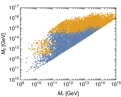
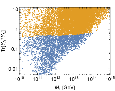
Figure 1: Scatter plot of all the points in our scan that lead to successful leptogenesis. Points in orange correspond to the points where any of the Lagrangian coupling constants become non-perturbative below the Planck scale and/or lead to a metastable EW vacuum with a lifetime smaller than the age of the Universe. Points in blue satisfy these constraints up to the Planck scale as well as leading to successful leptogenesis.

A detailed RG study of the Higgs potential in the SM has shown that at high scales the quartic coupling turns negative and the potential develops a new minimum Degrassi:2012ry ; Buttazzo:2013uya , for earlier related work on this topic see Lindner:1985uk ; Sher:1988mj . Taking the central values for measurements of the Higgs and the top mass, this secondary vacuum is deeper than the electroweak vacuum and hence, given sufficient time, there is a chance the Higgs field will tunnel into it. Requiring the age of the Universe to be larger than the lifetime of the electroweak vacuum implies a lower bound for negative values of $\lambda_{\rm eff}(\mu)$ Buttazzo:2013uya

$$|\lambda_{\rm eff}(\mu)|>\frac{2\pi^{2}}{3}\frac{1}{\ln(\tau\mu)},$$ (15)

where $\tau=4.35\times 10^{17}$ s is the age of the Universe Ade:2015xua . Using the one-loop RG improved Higgs potential and the two-loop $\beta$-functions with the most recent measurements for the top and the Higgs mass we find that $\lambda_{\rm eff}$ becomes negative at $\mu_{\rm inst}\!\approx\!5.2\times 10^{11}$ GeV in the SM.

Although non-perturbatively it is possible to show the gauge-independence of tunneling rates by applying Nielsen identities Nielsen:1975fs to the false-vacuum effective action Plascencia:2015pga , it appeared that in perturbative calculations the lifetime of the electroweak vacuum displayed gauge-dependence Patel:2011th ; DiLuzio:2014bua ; Lalak:2016zlv . There has been recent progress in performing a perturbative calculation of the decay rate that have resolved these issues Andreassen:2017rzq ; Chigusa:2017dux . In this work, we use the Landau gauge; however, we anticipate our conclusions not to change for a different choice of gauge-fixing.

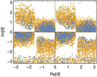
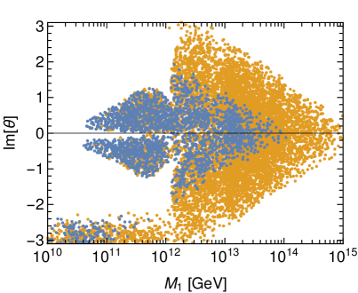
Figure 2: The colouring of the points is the same as in Fig. 1. We display the dependence on the real and imaginary part of the complex angle that enters in the $R$ matrix.

The initial conditions of the RG running are taken at $\mu\!=\!M_{t}$ and we use the central value of the top quark mass from recent measurements performed by ATLAS and CMS, $M_{t}\!=\!172.5$ GeV ATLAS:2017lqh ; Menke:11 . We take $M_{W}\!=\!80.384$ GeV and $M_{h}\!=\!125.09$ GeV for the pole mass of the $W$ and the Higgs bosons respectively and $\alpha_{3}(M_{Z})\!=\!0.1184$ for the strong coupling constant Patrignani:2016xqp . We complete the calculations using the next-to-next-to-leading order initial values for the SM couplings as given in Ref. Buttazzo:2013uya

$$g_{3}(\mu\!=\!M_{t}) =1.1666+0.00314\frac{\alpha_{3}(M_{Z})-0.1184}{0.0007}-0.00046\left(\frac{M_{t}}{\text{GeV}}-173.1\right),$$

$$g_{2}(\mu\!=\!M_{t}) =0.64779+0.00004\left(\frac{M_{t}}{\text{GeV}}-173.34\right)+0.00011\frac{M_{W}-80.384\text{ GeV}}{0.014\text{ GeV}},$$

$$g_{Y}(\mu\!=\!M_{t}) =0.35830+0.00011\left(\frac{M_{t}}{\text{GeV}}-173.34\right)-0.00020\frac{M_{W}-80.384\text{ GeV}}{0.014\text{ GeV}},$$

$$y_{t}(\mu\!=\!M_{t}) =0.93690+0.00556\left(\frac{M_{t}}{\text{GeV}}-173.34\right)-0.00042\frac{\alpha_{3}(M_{Z})-0.1184}{0.0007},$$

$$\lambda_{H}(\mu\!=\!M_{t}) =0.12604+0.00206\left(\frac{M_{h}}{\text{GeV}}-125.15\right)-0.00004\left(\frac{M_{t}}{\text{GeV}}-173.34\right).$$

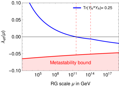
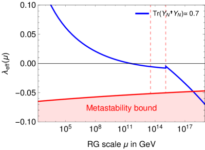
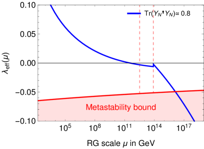
Figure 3: RG running of the effective Higgs quartic coupling as a function of the RG scale for points that lead to successful leptogenesis in the type-I seesaw mechanism. The red shaded region corresponds to the region where the lifetime of the EW vacuum is smaller than the age of the Universe. The dashed vertical lines correspond to the masses of $N_{1}$ and $N_{2}$. We show the running for different values of ${\rm Tr}[Y_{N}^{\dagger}Y_{N}]$ at the seesaw scale.

We present our results in Figs. 1-2. As can be seen in the left panel of Fig. 1, the region with smaller $M_{i}$ is less populated compared to larger $M_{i}$. This is expected since the CP-asymmetry in the decays of the heavy Majorana neutrino is proportional to its mass, $M_{1}$. As we require the model to be UV-robust up to the Planck scale we find an upper bound on the lightest right-handed Majorana neutrino $M_{1}\!\lesssim\!1.2\times 10^{14}$ GeV, this is similar to the one found in RG studies of the type-I seesaw without considering leptogenesis Casas:1999cd ; EliasMiro:2011aa . We also find an upper bound on the the mass splitting for $M_{1}>10^{13}$ GeV, namely $\Delta M_{12}/M_{1}\!\equiv\!(M_{2}-M_{1})/M_{1}\lesssim 10^{2}$ must be satisfied. The bounds we provide are conservative, in the sense that by taking a non-zero mass for the lightest active neutrino they will only become stronger. This is due to the seesaw relation in which larger values for $m_{1}$ require larger Yukawa couplings.

The right panel in Fig. 1 shows a scatter plot of $M_{1}$ versus ${\rm Tr}[Y_{N}^{\dagger}Y_{N}]$ where the values for the latter are computed at the seesaw scale. This plot shows that there is an upper bound ${\rm Tr}[Y_{N}^{\dagger}Y_{N}]\lesssim 0.66$. This bound does not significantly differ from the one found in Refs. Khan:2012zw ; Rose:2015fua for the low-scale inverse seesaw mechanism. This is because neutrino Yukawas $\sim 0.5$ have a drastic effect in driving $\lambda_{\rm eff}$ below the metastability bound. In Fig. 3 we present the running of $\lambda_{\rm eff}(\mu)$ for different values of ${\rm Tr}[Y_{N}^{\dagger}Y_{N}]$. As can be seen, for larger values of the neutrino Yukawa couplings, the effective Higgs quartic quickly crosses into the metastability bound.

In the left panel of Fig. 2, we display the points leading to successful leptogenesis in the $\text{Im}[\theta]$–$\text{Re}[\theta]$ plane. The periodic behaviour in $\text{Re}[\theta]$ may be inferred as the analytic forms of the washout, projection matrices and CP-asymmetries are all trigonometric functions of $\text{Re}[\theta]$. This periodic behaviour we observe concurs with the results of Antusch:2011nz . In spite of this periodicity in $\text{Re}[\theta]$, the constraints from vacuum stability and perturbativity are not sensitive to the absolute magnitude of this parameter.

In the right panel of Fig. 2, we observe that for $M_{1}\gtrsim 10^{12}$ GeV, there is a preference for small ${\rm Im}[\theta]$. This is because as $M_{1}$ is increased, ${\rm Im}[\theta]$ cannot grow too large (given that Yukawa couplings are exponentially enhanced with respect to this parameter) as this would result in the Yukawa matrix entries becoming non-perturbative. Although there are some data points that satisfy all our conditions with large ${\rm Im}[\theta]$ around $M_{1}\sim 10^{9}$ GeV, we find that, in general, $|{\rm Im}[\theta]|\lesssim 2$ is preferred. Ignoring effects from quantum gravity, a large portion of the points, close to 75$\%$, that satisfy perturbativity and vacuum stability up to the Planck scale, also satisfy these constraints up to the Landau pole of the hypercharge $\sim 10^{40}$ GeV.

4.2 Asymptotically Safe $\,{\rm SU}(3)_{c}$ and Leptogenesis

In the SM, the $\beta$-function of the strong coupling is negative, and therefore, the coupling decreases at higher energies Gross:1973id ; Politzer:1973fx . This property, known as asymptotic freedom, implies that quantum chromodynamics (QCD) is well-defined at arbitrarily short distances. Despite this, the running of $g_{3}$ has only been measured up to the TeV scale Bethke:2015etp and the addition of new coloured particles could lead to the loss of this property. However, the possibility arises in which the strong gauge coupling reaches an interacting ultraviolet fixed point, as proposed in Sannino:2015sel . Motivated by recent progress in constructing extensions of the Standard Model where at least one of the couplings becomes asymptotically safe, in this Section, we consider an extension of the SM in which QCD becomes asymptotically safe, rather than asymptotically free, in the UV. This is an alternative scenario where QCD is also well-defined at arbitrarily short distances and its cosmological consequences remain relatively unexplored. For this reason we study its implications on leptogenesis with a type-I seesaw mechanism.

Asymptotic safety is achieved when the couplings in a model reach an interacting ultraviolet fixed point. These fixed points $g^{*}_{i}$ correspond to the zeros of the $\beta$-function $\beta_{i}(g^{*}_{i})=0$. Asymptotic safety was recently shown to exist for gauge-Yukawa theories in a perturbative manner Litim:2014uca and has attracted recent attention Esbensen:2015cjw ; Molgaard:2016bqf ; Pelaggi:2017wzr ; Abel:2017ujy ; Bond:2017lnq ; Abel:2017rwl ; Bond:2017suy ; Bond:2017tbw . Theorems for weakly interacting theories with asymptotic safety have been established in Bond:2016dvk ; Bond:2018oco . In Bond:2017wut , the authors provide a prescription for constructing extensions of the SM in which the weak and strong coupling constants reach perturbative fixed points in the UV, but the hypercharge still suffers from a Landau pole.

An alternative approach to achieve an interacting UV-fixed point for a gauge coupling, associated to the gauge group $G$, is to add a large number ($N_{F}$) of fermions charged under $G$ and perform a $1/N_{F}$ expansion in the computation of the $\beta$-functions PalanquesMestre:1983zy ; Gracey:1996he ; Holdom:2010qs . Recently, the large-$N_{F}$ resummed contributions to the RG equations were computed in Antipin:2018zdg for generic semi-simple groups. In Mann:2017wzh , a large number of vector-like fermions were added to the SM in order to ensure the asymptotic safety of the gauge couplings; nevertheless, this calculation was completed without the inclusion of the large-$N_{F}$ resummation for the Yukawa and the Higgs quartic.

The large-$N_{F}$ resummation was performed for a Yukawa coupling in Kowalska:2017pkt ; Pelaggi:2017abg . In the latter work, the resummation was also computed for a scalar quartic coupling. These results were applied in Pelaggi:2017abg to extensions of the SM by a large number $N_{F}$ of charged fermions in order to make the strong or the weak gauge coupling asymptotically safe in the UV. Nonetheless, in that study it was shown that when one makes the hypercharge coupling safe in the UV, the Higgs quartic is driven to large non-perturbative values. This is because the location of the pole in the resummed functions for the Yukawa and the scalar quartic has the same location as the one in the Abelian case.

We now proceed to study a model where we add a large number ($N_{F}$) of coloured fermions in order to make the $\,{\rm SU}(3)_{c}$ coupling asymptotically safe and study the validity of a type-I leptogenesis scenario up to the scale at which the hypercharge develops a Landau pole $\sim 10^{40}$ GeV. With $N_{F}$ flavours of vector-like coloured fermions, the UV fixed point for the strong gauge coupling in the SM is given by,

$$g_{3}^{*}=\frac{4\pi}{\sqrt{\Delta b_{3}}},\hskip 28.45274pt{\rm and}\hskip 28.45274pt\Delta b_{3}=\frac{2}{3}N_{F}S_{R_{3}}D_{R_{2}},$$ (16)

where $\Delta b_{3}$ is the one-loop coefficient for Dirac fermions in the representation $R_{i}$, dimension $D_{R_{i}}$ and Dynkin index $S_{R_{i}}$. The large-$N_{F}$ resummed $\beta$-function has a pole at $g_{3}^{*}\!=\!4\pi/\sqrt{\Delta b_{3}}$ where it diverges to negative infinity. Before reaching the pole, this resummed contribution cancels out the one-loop contribution and the $\beta$-function becomes zero. For a review on the large-$N_{F}$ expansion we refer the reader to Ref. Holdom:2010qs .

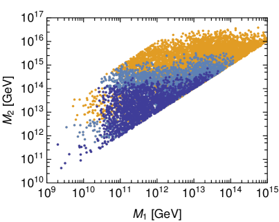
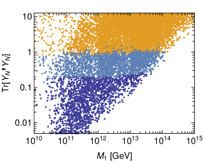
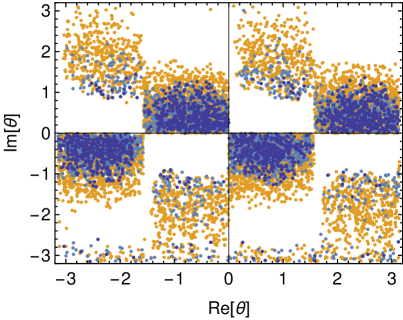
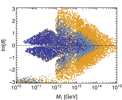
Figure 4: Scatter plot for all the points that lead to successful leptogenesis with an asymptotically safe $\,{\rm SU}(3)_{c}$. Points in orange correspond to the points where any of the Lagrangian coupling constants become non-perturbative at some high energy scale and/or lead to a metastable EW vacuum with a lifetime smaller than the age of the Universe. Points in blue satisfy the perturbativity condition and the EW vacuum is metastable. For points in dark blue, the electroweak vacuum is absolutely stable. The RG study is performed up to $10^{40}$ GeV.

In order to perform the RG study, we consider the one-loop $\beta$-functions with the resummed contribution at leading order in $1/N_{F}$ which we present in Appendix B. For this scenario, we assume that gravity will only have subleading effects on the RG running of the couplings above the Planck scale, similar to the approach of softened gravity presented in Ref. Giudice:2014tma . In lack of a theory of quantum gravity, we will allow ourselves such speculation.

At one-loop the $N_{F}$ fermions give a positive contribution to the running of $g_{3}$ so that $g_{3}$ increases before reaching its fixed point, i.e. $g_{3}^{*}\geq g_{3}(M_{t})$. Therefore, the negative contribution from $g_{3}$ to the running of $y_{t}$ can be larger, driving $y_{t}$ to smaller values compared to the SM case. This helps with the stability of the EW vacuum. As was shown in Ref. Pelaggi:2017abg , the addition of $7\leq N_{F}\leq 13$ Majorana colour octets stabilises the EW vacuum. Here the lower bound derives from the requirement of convergence in the $1/N_{F}$ expansion for fermions in the adjoint representation Antipin:2017ebo . The achievement of vacuum stability provides a further motivation to consider such a scenario.

For our numerical scan we consider a scenario with $N_{F}=13$ Majorana colour octets with common masses $M_{F}=5$ TeV. This corresponds to $\Delta b_{3}=26$ and $g_{3}^{*}\simeq 2.5$, for the one-loop coefficient and the fixed point for the strong coupling respectively. The calculation of the baryon asymmetry follows the same procedure from before with the exception that the number of relativistic degrees of freedom is now $g_{*}\!=\!288.75$ due to the inclusion of the new vector-like fermions. The modification of $g_{*}$ must be accounted for in the density matrix equations; naturally, the Hubble rate is altered and this affects the decay parameter, $K_{1}$, (as detailed in Appendix A) which in turn affects the decay and washout of the lepton asymmetry. In addition, the Hubble-normalised thermal width of the tau and muon charged leptons are changed accordingly. The effect of an enlarged $g_{*}$ causes suppression of the decay parameter and the washout by a factor of a few. The corresponding results can be seen in Figs. 4.

We would like to highlight the similarities and differences in the parameter space between the minimal type-I seesaw leptogenesis scenario and the large-$N_{F}$ case considered here. In the latter case, there exists a region in parameter space where the Higgs potential becomes absolutely stable. In addition, the bound on the neutrino Yukawa couplings is relaxed from ${\rm Tr}[Y_{N}^{\dagger}Y_{N}]\lesssim 0.66$ (Fig. 1) in the minimal case to ${\rm Tr}[Y_{N}^{\dagger}Y_{N}]\lesssim 1.51$ in the large-$N_{F}$ case (Fig. 4). The upper bound on $M_{1}$ is the same in both scenarios.

Finally, we note that the addition of a large number of fermions ($N_{F}$) that possess weak charge can make the $\,{\rm SU}(2)_{L}$ gauge coupling asymptotically safe. Nevertheless, in this scenario the Higgs quartic coupling violates the metastability bound Pelaggi:2017abg and the addition of heavy Majorana neutrinos, which give a negative contribution to the the RG equation of $\lambda_{H}$, cannot improve this situation. Hence, we do not consider this scenario any further.

5 Conclusions

The origin of neutrino masses and the baryon asymmetry of the Universe remain two experimentally observed phenomena that cannot be explained by the Standard Model. One of the most minimal solutions to these shortcomings is the introduction of three heavy Majorana neutrinos to the SM particle spectrum. As a consequence, the active neutrinos acquire their masses via a type-I seesaw mechanism and the baryon asymmetry is produced via CP-violating, out-of-equilibrium decays of the lightest sterile neutrino.

It is well known that in order to address the baryon asymmetry of the Universe using thermal leptogenesis with a hierarchical mass spectrum in the heavy neutrino sector requires $M_{1}\gtrsim 10^{9}$ GeV. This means that the Yukawa couplings can be relatively large and hence the model may suffer from non-perturbative couplings or violate the condition of metastability for the electroweak vacuum. In the present work we have discussed the self-consistency of thermal leptogenesis up to high scales.

We started by performing a numerical scan in order to find the points that produce sufficient baryon asymmetry, where each point in our scan reproduces the central values for the measured neutrino mass differences (with normal ordering) and mixing angles. In order to compute the baryon asymmetry we have solved the density matrix equations that are valid in the whole range of masses studied. We subsequently solved the RG equations for these points in order to assess the validity of the model up to the Planck scale.

In summary, we have identified the region of parameter space in minimal thermal leptogenesis that allow for the (i) electroweak vacuum to remain metastable and (ii) for all the couplings in the model to remain perturbative up to the Planck scale. We find an upper bound on the neutrino Yukawa matrix and on the mass of the lightest right handed neutrino, ${\rm Tr}[Y_{N}^{\dagger}Y_{N}]\lesssim 0.66$ and $M_{1}\lesssim 10^{14}$ GeV respectively. There is also a strong preference for $|{\rm Im}[\theta]|\lesssim 2$, where $\theta$ is the complex angle that parametrises the $R$ matrix. Detailed results can be seen in Figs. 1-2. Three quarters of the points that satisfy these constraints up to the Planck scale also satisfy the constraints up to the scale at which the hypercharge develops a Landau pole $\sim 10^{40}$ GeV. Motivated by this and recent progress in making the gauge couplings in the SM asymptotically safe in the UV, we also studied a scenario where the $\,{\rm SU}(3)_{c}$ coupling becomes asymptotically safe and found constraints in the parameter space that leads to successful leptogenesis. However, this minimal model still suffers from a Landau pole developed by the hypercharge coupling. It remains a future task to address this issue.

Appendix A Details of Kinetic Equations

In this Appendix, we provide the formulae used within the density matrix equation Eq. (6). The decay and washout terms are given by

$$D_{1}(z)=K_{1}z\frac{\mathcal{K}_{1}(z)}{\mathcal{K}_{2}(z)},\quad\mathcal{W}_{1}(z)=\frac{1}{4}K_{1}\mathcal{K}_{1}(z)z^{3},$$ (17)

where $\mathcal{K}_{1}$ and $\mathcal{K}_{2}$ are modified Bessel functions of the second kind with the decay asymmetry $K_{1}$ written as

$$K_{1}\equiv\frac{\tilde{\Gamma}_{i}}{H(T=M_{1})},\quad\tilde{\Gamma}_{1}=\frac{M_{1}\left(Y^{\dagger}Y\right)_{11}}{8\pi}.$$ (18)

These CP-asymmetry parameters may be written as Covi:1996wh ; Blanchet:2011xq ; Abada:2006ea ; DeSimone:2006nrs

$$\epsilon^{(i)}_{\alpha\beta}=\frac{3}{32\pi\left(Y^{\dagger}Y\right)_{ii}}\sum_{j\neq i} \Bigg{\{}i[Y_{\alpha i}Y^{*}_{\beta j}(Y^{\dagger}Y)_{ji}-Y_{\beta i}Y^{*}_{\alpha j}(Y^{\dagger}Y)_{ij}]f_{1}\left(\frac{x_{j}}{x_{i}}\right)$$ (19)

$$+i[Y_{\alpha i}Y^{*}_{\beta j}(Y^{\dagger}Y)_{ij}-Y_{\beta i}Y^{*}_{\alpha j}(Y^{\dagger}Y)_{ji}]f_{2}\left(\frac{x_{j}}{x_{i}}\right)\Bigg{\}},$$

where

$$f_{1}\left(\frac{x_{j}}{x_{i}}\right)=\frac{\xi\left(\frac{x_{j}}{x_{i}}\right)}{\sqrt{\frac{x_{j}}{x_{i}}}},\quad f_{2}\left(\frac{x_{j}}{x_{i}}\right)=\frac{2}{3\left(\frac{x_{j}}{x_{i}}-1\right)},\quad\xi\left(x\right)=\frac{2}{3}x\left[\left(1+x\right)\ln\left(\frac{1+x}{x}\right)-\frac{2-x}{1-x}\right].$$ (20)

The density matrix equations of Eq. (6) may be expanded straightforwardly in terms of the flavour indices:

$$\frac{dn_{N_{1}}}{dz} =-D_{1}(n_{N_{1}}-n^{\text{eq}}_{N_{1}})$$ (21)

$$\frac{dn_{\tau\tau}}{dz} =\epsilon^{(1)}_{\tau\tau}D_{1}(n_{N_{1}}-n^{\text{eq}}_{N_{1}})-\mathcal{W}_{1}\left\{\left|Y_{\tau 1}\right|{}^{2}n_{\tau\tau}+\text{Re}\left[Y^{*}_{\tau 1}\left(Y_{e1}n_{\tau e}+Y_{\mu 1}n_{\tau\mu}\right)\right]\right\}$$

$$\frac{dn_{\mu\mu}}{dz} =\epsilon^{(1)}_{\mu\mu}D_{1}(n_{N_{1}}-n^{\text{eq}}_{N_{1}})-\mathcal{W}_{1}\left\{\left|Y_{\mu 1}\right|{}^{2}n_{\mu\mu}+\text{Re}\left[Y^{*}_{\mu 1}\left(Y_{e1}n_{\mu e}+Y_{\tau 1}n^{*}_{\tau\mu}\right)\right]\right\}$$

$$\frac{dn_{ee}}{dz} =\epsilon^{(1)}_{ee}D_{1}(n_{N_{1}}-n^{\text{eq}}_{N_{1}})-\mathcal{W}_{1}\left\{\left|Y_{e1}\right|{}^{2}n_{ee}+\text{Re}\right[Y^{*}_{e1}\left(Y_{\mu 1}n^{*}_{\mu e}+Y_{\tau 1}n^{*}_{\tau e}\right)\left]\right\}$$

$$\frac{dn_{\tau\mu}}{dz} =\epsilon^{(1)}_{\tau\mu}D_{1}(n_{N_{1}}-n^{\text{eq}}_{N_{1}})-\left(\frac{\text{Im}\left(\Lambda_{\tau}\right)}{Hz}+\frac{\text{Im}\left(\Lambda_{\mu}\right)}{Hz}\right)n_{\tau\mu}$$

$$-\frac{\mathcal{W}_{1}}{2}\left\{n_{\tau\mu}\left(\left|Y_{\tau 1}\right|{}^{2}+\left|Y_{\mu 1}\right|{}^{2}\right)+Y^{*}_{\mu 1}Y_{\tau 1}\left(n_{\tau\tau}+n_{\mu\mu}\right)+Y^{*}_{e1}Y_{\tau 1}n^{*}_{\mu e}+Y^{*}_{\mu 1}Y_{e1}n_{\tau e}\right\}$$

$$\frac{dn_{\tau e}}{dz} =\epsilon^{(1)}_{\tau e}D_{1}(n_{N_{1}}-n^{\text{eq}}_{N_{1}})-\frac{\text{Im}\left(\Lambda_{\tau}\right)}{Hz}n_{\tau e}$$

$$-\frac{\mathcal{W}_{1}}{2}\left\{n_{\tau e}\left(\left|Y_{e1}\right|{}^{2}+\left|Y_{\tau 1}\right|{}^{2}\right)+Y^{*}_{e1}Y_{\tau 1}\left(n_{ee}+n_{\tau\tau}\right)+Y^{*}_{\mu 1}Y_{\tau 1}n_{\mu e}+Y^{*}_{e1}Y_{\mu 1}n_{\tau\mu}\right\}$$

$$\frac{dn_{\mu e}}{dz} =\epsilon^{(1)}_{\mu e}D_{1}(n_{N_{1}}-n^{\text{eq}}_{N_{1}})-\frac{\text{Im}\left(\Lambda_{\mu}\right)}{Hz}n_{\mu e}$$

$$-\frac{\mathcal{W}_{1}}{2}\left\{n_{\mu e}\left(\left|Y_{e1}\right|{}^{2}+\left|Y_{\mu 1}\right|{}^{2}\right)+Y^{*}_{e1}Y_{\mu 1}\left(n_{ee}+n_{\mu\mu}\right)+Y^{*}_{e1}Y_{\tau 1}n^{*}_{\tau\mu}+Y^{*}_{\tau 1}Y_{\mu 1}n_{\tau e}\right\},$$

where the total number density of the lepton asymmetry is given by the trace of this matrix, $n_{B-L}=n_{ee}+n_{\mu\mu}+n_{\tau\tau}$. In order to compare to measurement of the baryon-to-photon ratio, $\eta_{B}$, from cosmic microwave background measurements Ade:2015xua , we have to ensure $n_{B-L}$ is properly rescaled by a factor of 0.0096 which accounts for the sphaleron conversion factor (28/79) and the number density of comoving photons after recombination Buchmuller:2004nz . The off-diagonal number densities encode the quantum correlations between flavours differing flavours of charged leptons within the thermal bath; $n_{\alpha\beta}$ term describes the number density of $\ell_{\alpha}$ being converted to $\overline{\ell_{\beta}}$.

$\Lambda_{\alpha}$ represents the self energy of the $\alpha$-flavoured charged lepton in the thermal bath. The imaginary (real) part of the self energy is the thermal width (mass) of the lepton and will be important in describing the transition between various flavour regimes of leptogenesis. Physically, the thermal width is related to the mean free path of the lepton in the thermal bath.

At high temperatures, ($T>10^{12}$ GeV), the Yukawa interactions of all the charged leptons are out of equilibrium and hence there is only one effective flavour of charged lepton. As the Universe expands and cools, the interaction rates mediated by the SM $\tau$ Yukawa coupling come into thermal equilibrium. At such temperatures the Universe can now distinguish flavour $\tau$ from $\tau^{\perp}$, where $\tau^{\perp}$ is a coherent superposition of $e$ and $\mu$ flavour. As such, the $\tau$-state has broken the coherence of the $N_{1}$ decays. $\text{Im}(\Lambda_{\tau})$ enters into the Boltzmann equations in the following way

$$\frac{\text{Im}(\Lambda_{\tau})}{Hz}\quad\text{where}\quad H(z)\sim 1.66\sqrt{g^{*}}\frac{M^{2}_{1}}{M_{\rm PL}}\frac{1}{z^{2}}\implies zH(z)=1.66g^{*}\frac{M^{2}_{1}}{M_{\rm PL}}\frac{1}{z}$$ (22)

where $z=\frac{M_{1}}{T}$. The thermal width of the $\tau$ takes the following form Blanchet:2011xq

$$\text{Im}(\Lambda_{\tau})=8\times 10^{-3}f^{2}_{\tau}T.$$ (23)

Using (22) and (23) we find,

$$\frac{\text{Im}(\Lambda_{\tau})}{Hz}=\frac{8\times 10^{-3}f^{2}_{\tau}M_{\rm PL}}{1.66\sqrt{g^{*}}M_{1}},$$ (24)

where $M_{\rm PL}\!=\!1.22\times 10^{19}$ GeV and $g^{*}\!=\!106.75$. Note that $f_{\tau}$ is the $\tau$ charged lepton Yukawa coupling

$$m_{\tau}=f_{\tau}v\implies f_{\tau}=\frac{m_{\tau}}{v}=\frac{1.777}{174}\sim 0.01,$$ (25)

where all the units above are in GeV. We can rewrite (24)

$$\frac{\text{Im}(\Lambda_{\tau})}{Hz}=4.85\times 10^{-8}\frac{M_{\rm PL}}{M_{1}}.$$ (26)

As $\text{Im}(\Lambda_{\alpha})/Hz\propto 1/M_{1}$, the lower the scale of leptogenesis the larger impact the Hubble normalised thermal width. From Eq. (6), it can be seen that $\text{Im}(\Lambda)$ acts in competition with the off-diagonal number densities. At lower values of $M_{1}$, the interaction rates of mediated by the SM charged lepton Yukawa couplings become increasingly significant. This means the $\tau$ and $\overline{\tau}$ in the thermal bath are more likely to find each other and annihilate via a Higgs than be converted to an $e$ or $\mu$ via a heavy Majorana neutrino. This implies the flavour correlations between the flavours of charged leptons become less significant for smaller $M_{1}$.

Appendix B Resummed Contribution to the RGEs with a Large Number of Flavours

We consider an extension to the SM where we introduce a large number of coloured particles, this implies that only the running of $g_{3}$ and $y_{t}$ will be modified by the resummation at leading order in $1/N_{F}$. The resummed $\beta$-function for the strong gauge coupling can be written as,

$$\frac{\partial\alpha_{3}}{\partial\ln\mu}=-7\frac{\alpha_{3}^{2}}{2\pi}+\Delta b_{3}\frac{\alpha_{3}^{2}}{2\pi}+F_{3}\left(A\right)\frac{\alpha_{3}^{2}}{2\pi},$$ (27)

where $A\equiv\Delta b_{3}\alpha_{3}/(4\pi)$, $\alpha_{3}=g_{3}^{2}/(4\pi)$ and $\Delta b_{3}$ is the one-loop contribution from the $N_{F}$ fermions and is given in Eq. (16). The resummed contribution is given by PalanquesMestre:1983zy ; Gracey:1996he ; Holdom:2010qs ,

$$F_{3}(A) =\int_{0}^{A}I_{1}(x)I_{3}(x)\,dx,$$ (28)

$$I_{1}(x) \equiv\frac{(1+x)(2x-1)^{2}(2x-3)^{2}\sin^{3}(\pi x)\Gamma(x-1)^{2}\Gamma(-2x)}{\pi^{3}(x-2)},$$ (29)

$$I_{3}(x) \equiv\frac{4}{3}+\frac{3(20-43x+32x^{2}-14x^{3}+4x^{4})}{2(2x-1)(2x-3)(1-x^{2})}.$$ (30)

The $\beta$-function for the top Yukawa coupling is modified as follows,

$$(4\pi)^{2}\frac{dy_{t}}{d\ln\mu}=\frac{9}{2}y_{t}^{3}-y_{t}\left(8g_{3}^{2}R_{y}(A_{3})+\frac{9}{4}g_{2}^{2}+\frac{17}{12}g_{Y}^{2}\right),$$ (31)

where the resummed function is given by,

$$R_{y}(A)=\frac{2(3-2A)^{2}(2-A)\sin(\pi A)\Gamma(2-2A)}{9\pi A\Gamma(3-A)^{2}},$$ (32)

and hence at the fixed point, where $\alpha_{3}^{*}=4\pi/\Delta b_{3}$, $R_{y}(1)=1/9$. For details on the class of diagrams that contribute to the resummation and a detailed derivation of the resummed function $R_{y}(A)$ we refer the reader to Refs. Kowalska:2017pkt ; Pelaggi:2017abg . For the scenario considered in Section 4.2 we solve the one-loop RG equations (8)-(11) with the equations for $g_{3}$ and $y_{t}$ replaced by (27) and (31) respectively.

References

- (1) P. Minkowski, at a Rate of One Out of Muon Decays?, Phys. Lett. B67 (1977) 421–428.
- (2) T. Yanagida, HORIZONTAL SYMMETRY AND MASSES OF NEUTRINOS, Conf. Proc. C7902131 (1979) 95–99.
- (3) M. Gell-Mann, P. Ramond and R. Slansky, Complex Spinors and Unified Theories, Conf. Proc. C790927 (1979) 315–321, [1306.4669].
- (4) R. N. Mohapatra and G. Senjanovic, Neutrino Mass and Spontaneous Parity Violation, Phys. Rev. Lett. 44 (1980) 912.
- (5) M. Fukugita and T. Yanagida, Baryogenesis Without Grand Unification, Phys. Lett. B174 (1986) 45–47.
- (6) J. A. Casas, V. Di Clemente, A. Ibarra and M. Quiros, Massive neutrinos and the Higgs mass window, Phys. Rev. D62 (2000) 053005, [hep-ph/9904295].
- (7) J. Elias-Miro, J. R. Espinosa, G. F. Giudice, G. Isidori, A. Riotto and A. Strumia, Higgs mass implications on the stability of the electroweak vacuum, Phys. Lett. B709 (2012) 222–228, [1112.3022].
- (8) C.-S. Chen and Y. Tang, Vacuum stability, neutrinos, and dark matter, JHEP 04 (2012) 019, [1202.5717].
- (9) W. Rodejohann and H. Zhang, Impact of massive neutrinos on the Higgs self-coupling and electroweak vacuum stability, JHEP 06 (2012) 022, [1203.3825].
- (10) G. Bambhaniya, P. Bhupal Dev, S. Goswami, S. Khan and W. Rodejohann, Naturalness, Vacuum Stability and Leptogenesis in the Minimal Seesaw Model, Phys. Rev. D95 (2017) 095016, [1611.03827].
- (11) P. Ghosh, A. K. Saha and A. Sil, Study of Electroweak Vacuum Stability from Extended Higgs Portal of Dark Matter and Neutrinos, Phys. Rev. D97 (2018) 075034, [1706.04931].
- (12) G. Ballesteros, J. Redondo, A. Ringwald and C. Tamarit, Standard Model axion seesaw Higgs portal inflation. Five problems of particle physics and cosmology solved in one stroke, JCAP 1708 (2017) 001, [1610.01639].
- (13) A. Salvio, A Simple Motivated Completion of the Standard Model below the Planck Scale: Axions and Right-Handed Neutrinos, Phys. Lett. B743 (2015) 428–434, [1501.03781].
- (14) A. Pilaftsis and T. E. J. Underwood, Resonant leptogenesis, Nucl. Phys. B692 (2004) 303–345, [hep-ph/0309342].
- (15) F. Vissani, Do experiments suggest a hierarchy problem?, Phys. Rev. D57 (1998) 7027–7030, [hep-ph/9709409].
- (16) M. Farina, D. Pappadopulo and A. Strumia, A modified naturalness principle and its experimental tests, JHEP 08 (2013) 022, [1303.7244].
- (17) S. Khan, S. Goswami and S. Roy, Vacuum Stability constraints on the minimal singlet TeV Seesaw Model, Phys. Rev. D89 (2014) 073021, [1212.3694].
- (18) L. Delle Rose, C. Marzo and A. Urbano, On the stability of the electroweak vacuum in the presence of low-scale seesaw models, JHEP 12 (2015) 050, [1506.03360].
- (19) M. Lindner, H. H. Patel and B. Radovčić, Electroweak Absolute, Meta-, and Thermal Stability in Neutrino Mass Models, Phys. Rev. D93 (2016) 073005, [1511.06215].
- (20) L. Di Luzio, R. Gröber and M. Spannowsky, Maxi-sizing the trilinear Higgs self-coupling: how large could it be?, Eur. Phys. J. C77 (2017) 788, [1704.02311].
- (21) S. Yu. Khlebnikov and M. E. Shaposhnikov, The Statistical Theory of Anomalous Fermion Number Nonconservation, Nucl. Phys. B308 (1988) 885–912.
- (22) S. Davidson and A. Ibarra, A Lower bound on the right-handed neutrino mass from leptogenesis, Phys. Lett. B535 (2002) 25–32, [hep-ph/0202239].
- (23) K. Moffat, S. Pascoli, S. T. Petcov, H. Schulz and J. Turner, Three-Flavoured Non-Resonant Leptogenesis at Intermediate Scales, 1804.05066.
- (24) K. Agashe, P. Du, M. Ekhterachian, C. S. Fong, S. Hong and L. Vecchi, Hybrid seesaw leptogenesis and TeV singlets, 1804.06847.
- (25) W. Buchmuller, P. Di Bari and M. Plumacher, Leptogenesis for pedestrians, Annals Phys. 315 (2005) 305–351, [hep-ph/0401240].
- (26) W. Buchmuller, P. Di Bari and M. Plumacher, Cosmic microwave background, matter - antimatter asymmetry and neutrino masses, Nucl. Phys. B643 (2002) 367–390, [hep-ph/0205349].
- (27) J. A. Casas and A. Ibarra, Oscillating neutrinos and muon —> e, gamma, Nucl. Phys. B618 (2001) 171–204, [hep-ph/0103065].
- (28) S. M. Bilenky, J. Hosek and S. T. Petcov, On Oscillations of Neutrinos with Dirac and Majorana Masses, Phys. Lett. 94B (1980) 495–498.
- (29) J. Schechter and J. W. F. Valle, Neutrino Masses in SU(2) x U(1) Theories, Phys. Rev. D22 (1980) 2227.
- (30) E. Molinaro and S. T. Petcov, The Interplay Between the ’Low’ and ’High’ Energy CP-Violation in Leptogenesis, Eur. Phys. J. C61 (2009) 93–109, [0803.4120].
- (31) I. Esteban, M. C. Gonzalez-Garcia, M. Maltoni, I. Martinez-Soler and T. Schwetz, Updated fit to three neutrino mixing: exploring the accelerator-reactor complementarity, JHEP 01 (2017) 087, [1611.01514].
- (32) A. Ibarra and G. G. Ross, Neutrino phenomenology: The Case of two right-handed neutrinos, Phys. Lett. B591 (2004) 285–296, [hep-ph/0312138].
- (33) S. Antusch, P. Di Bari, D. A. Jones and S. F. King, Leptogenesis in the Two Right-Handed Neutrino Model Revisited, Phys. Rev. D86 (2012) 023516, [1107.6002].
- (34) S. Blanchet, Dirac phase leptogenesis, J. Phys. Conf. Ser. 120 (2008) 022007, [0710.0570].
- (35) P. H. Frampton, S. L. Glashow and T. Yanagida, Cosmological sign of neutrino CP violation, Phys. Lett. B548 (2002) 119–121, [hep-ph/0208157].
- (36) S. F. King, Leptogenesis MNS link in unified models with natural neutrino mass hierarchy, Phys. Rev. D67 (2003) 113010, [hep-ph/0211228].
- (37) P. H. Chankowski and K. Turzynski, Limits on T(reh) for thermal leptogenesis with hierarchical neutrino masses, Phys. Lett. B570 (2003) 198–204, [hep-ph/0306059].
- (38) A. Abada, S. Davidson, A. Ibarra, F. X. Josse-Michaux, M. Losada and A. Riotto, Flavour Matters in Leptogenesis, JHEP 09 (2006) 010, [hep-ph/0605281].
- (39) S. Antusch, S. F. King and A. Riotto, Flavour-Dependent Leptogenesis with Sequential Dominance, JCAP 0611 (2006) 011, [hep-ph/0609038].
- (40) E. Molinaro and S. T. Petcov, A Case of Subdominant/Suppressed ’High Energy’ Contribution to the Baryon Asymmetry of the Universe in Flavoured Leptogenesis, Phys. Lett. B671 (2009) 60–65, [0808.3534].
- (41) A. Anisimov, S. Blanchet and P. Di Bari, Viability of Dirac phase leptogenesis, JCAP 0804 (2008) 033, [0707.3024].
- (42) S. Blanchet, P. Di Bari, D. A. Jones and L. Marzola, Leptogenesis with heavy neutrino flavours: from density matrix to Boltzmann equations, JCAP 1301 (2013) 041, [1112.4528].
- (43) R. Barbieri, P. Creminelli, A. Strumia and N. Tetradis, Baryogenesis through leptogenesis, Nucl. Phys. B575 (2000) 61–77, [hep-ph/9911315].
- (44) A. Abada, S. Davidson, F.-X. Josse-Michaux, M. Losada and A. Riotto, Flavor issues in leptogenesis, JCAP 0604 (2006) 004, [hep-ph/0601083].
- (45) A. De Simone and A. Riotto, On the impact of flavour oscillations in leptogenesis, JCAP 0702 (2007) 005, [hep-ph/0611357].
- (46) S. Blanchet, P. Di Bari and G. G. Raffelt, Quantum Zeno effect and the impact of flavor in leptogenesis, JCAP 0703 (2007) 012, [hep-ph/0611337].
- (47) R. Cooke, M. Pettini, R. A. Jorgenson, M. T. Murphy and C. C. Steidel, Precision measures of the primordial abundance of deuterium, Astrophys. J. 781 (2014) 31, [1308.3240].
- (48) Particle Data Group collaboration, C. Patrignani et al., Review of Particle Physics, Chin. Phys. C40 (2016) 100001.
- (49) Planck collaboration, P. A. R. Ade et al., Planck 2015 results. XIII. Cosmological parameters, Astron. Astrophys. 594 (2016) A13, [1502.01589].
- (50) I. Gogoladze, N. Okada and Q. Shafi, Higgs boson mass bounds in a type II seesaw model with triplet scalars, Phys. Rev. D78 (2008) 085005, [0802.3257].
- (51) B. He, N. Okada and Q. Shafi, 125 GeV Higgs, type III seesaw and gauge Higgs unification, Phys. Lett. B716 (2012) 197–202, [1205.4038].
- (52) J. Chakrabortty, M. Das and S. Mohanty, Constraints on TeV scale Majorana neutrino phenomenology from the Vacuum Stability of the Higgs, Mod. Phys. Lett. A28 (2013) 1350032, [1207.2027].
- (53) A. Kobakhidze and A. Spencer-Smith, Neutrino Masses and Higgs Vacuum Stability, JHEP 08 (2013) 036, [1305.7283].
- (54) C. Bonilla, R. M. Fonseca and J. W. F. Valle, Vacuum stability with spontaneous violation of lepton number, Phys. Lett. B756 (2016) 345–349, [1506.04031].
- (55) J. N. Ng and A. de la Puente, Electroweak Vacuum Stability and the Seesaw Mechanism Revisited, Eur. Phys. J. C76 (2016) 122, [1510.00742].
- (56) N. Haba, H. Ishida, N. Okada and Y. Yamaguchi, Vacuum stability and naturalness in type-II seesaw, Eur. Phys. J. C76 (2016) 333, [1601.05217].
- (57) I. Garg, S. Goswami, V. K. N. and N. Khan, Electroweak vacuum stability in presence of singlet scalar dark matter in TeV scale seesaw models, Phys. Rev. D96 (2017) 055020, [1706.08851].
- (58) D. Buttazzo, G. Degrassi, P. P. Giardino, G. F. Giudice, F. Sala, A. Salvio et al., Investigating the near-criticality of the Higgs boson, JHEP 12 (2013) 089, [1307.3536].
- (59) T. P. Cheng, E. Eichten and L.-F. Li, Higgs Phenomena in Asymptotically Free Gauge Theories, Phys. Rev. D9 (1974) 2259.
- (60) D. J. Gross and F. Wilczek, Ultraviolet Behavior of Nonabelian Gauge Theories, Phys. Rev. Lett. 30 (1973) 1343–1346.
- (61) H. D. Politzer, Reliable Perturbative Results for Strong Interactions?, Phys. Rev. Lett. 30 (1973) 1346–1349.
- (62) B. Grzadkowski and M. Lindner, Nonlinear Evolution of Yukawa Couplings, Phys. Lett. B193 (1987) 71.
- (63) Yu. F. Pirogov and O. V. Zenin, Two loop renormalization group restrictions on the standard model and the fourth chiral family, Eur. Phys. J. C10 (1999) 629–638, [hep-ph/9808396].
- (64) S. Antusch, J. Kersten, M. Lindner and M. Ratz, Neutrino mass matrix running for nondegenerate seesaw scales, Phys. Lett. B538 (2002) 87–95, [hep-ph/0203233].
- (65) J. A. Casas, J. R. Espinosa, A. Ibarra and I. Navarro, General RG equations for physical neutrino parameters and their phenomenological implications, Nucl. Phys. B573 (2000) 652–684, [hep-ph/9910420].
- (66) S. Antusch, J. Kersten, M. Lindner and M. Ratz, Running neutrino masses, mixings and CP phases: Analytical results and phenomenological consequences, Nucl. Phys. B674 (2003) 401–433, [hep-ph/0305273].
- (67) J. A. Casas, J. R. Espinosa and M. Quiros, Improved Higgs mass stability bound in the standard model and implications for supersymmetry, Phys. Lett. B342 (1995) 171–179, [hep-ph/9409458].
- (68) G. Degrassi, S. Di Vita, J. Elias-Miro, J. R. Espinosa, G. F. Giudice, G. Isidori et al., Higgs mass and vacuum stability in the Standard Model at NNLO, JHEP 08 (2012) 098, [1205.6497].
- (69) M. Lindner, Implications of Triviality for the Standard Model, Z. Phys. C31 (1986) 295.
- (70) M. Sher, Electroweak Higgs Potentials and Vacuum Stability, Phys. Rept. 179 (1989) 273–418.
- (71) N. K. Nielsen, On the Gauge Dependence of Spontaneous Symmetry Breaking in Gauge Theories, Nucl. Phys. B101 (1975) 173–188.
- (72) A. D. Plascencia and C. Tamarit, Convexity, gauge-dependence and tunneling rates, JHEP 10 (2016) 099, [1510.07613].
- (73) H. H. Patel and M. J. Ramsey-Musolf, Baryon Washout, Electroweak Phase Transition, and Perturbation Theory, JHEP 07 (2011) 029, [1101.4665].
- (74) L. Di Luzio and L. Mihaila, On the gauge dependence of the Standard Model vacuum instability scale, JHEP 06 (2014) 079, [1404.7450].
- (75) Z. Lalak, M. Lewicki and P. Olszewski, Gauge fixing and renormalization scale independence of tunneling rate in Abelian Higgs model and in the standard model, Phys. Rev. D94 (2016) 085028, [1605.06713].
- (76) A. Andreassen, W. Frost and M. D. Schwartz, Scale Invariant Instantons and the Complete Lifetime of the Standard Model, Phys. Rev. D97 (2018) 056006, [1707.08124].
- (77) S. Chigusa, T. Moroi and Y. Shoji, State-of-the-Art Calculation of the Decay Rate of Electroweak Vacuum in the Standard Model, Phys. Rev. Lett. 119 (2017) 211801, [1707.09301].
- (78) ATLAS collaboration, Measurement of the top quark mass in the lepton+jets channel from =8 TeV ATLAS data, ATLAS-CONF-2017-071 (2017) .
- (79) S. Menke, Measurements of the top quark mass using the CMS and ATLAS detectors at the LHC, Moriond-Electroweak (2018) .
- (80) S. Bethke, G. Dissertori and G. P. Salam, World Summary of (2015), EPJ Web Conf. 120 (2016) 07005.
- (81) F. Sannino, at LHC: Challenging asymptotic freedom, in Proceedings, High-Precision Measurements from LHC to FCC-ee: Geneva, Switzerland, October 2-13, 2015, pp. 11–19, 2015, 1511.09022.
- (82) D. F. Litim and F. Sannino, Asymptotic safety guaranteed, JHEP 12 (2014) 178, [1406.2337].
- (83) J. K. Esbensen, T. A. Ryttov and F. Sannino, Quantum critical behavior of semisimple gauge theories, Phys. Rev. D93 (2016) 045009, [1512.04402].
- (84) E. Mølgaard and F. Sannino, Asymptotically safe and free chiral theories with and without scalars, Phys. Rev. D96 (2017) 056004, [1610.03130].
- (85) G. M. Pelaggi, F. Sannino, A. Strumia and E. Vigiani, Naturalness of asymptotically safe Higgs, Front.in Phys. 5 (2017) 49, [1701.01453].
- (86) S. Abel and F. Sannino, Radiative symmetry breaking from interacting UV fixed points, Phys. Rev. D96 (2017) 056028, [1704.00700].
- (87) A. D. Bond and D. F. Litim, More asymptotic safety guaranteed, Phys. Rev. D97 (2018) 085008, [1707.04217].
- (88) S. Abel and F. Sannino, Framework for an asymptotically safe Standard Model via dynamical breaking, Phys. Rev. D96 (2017) 055021, [1707.06638].
- (89) A. D. Bond and D. F. Litim, Asymptotic safety guaranteed in supersymmetry, Phys. Rev. Lett. 119 (2017) 211601, [1709.06953].
- (90) A. D. Bond, D. F. Litim, G. Medina Vazquez and T. Steudtner, UV conformal window for asymptotic safety, Phys. Rev. D97 (2018) 036019, [1710.07615].
- (91) A. D. Bond and D. F. Litim, Theorems for Asymptotic Safety of Gauge Theories, Eur. Phys. J. C77 (2017) 429, [1608.00519].
- (92) A. D. Bond and D. F. Litim, Price of Asymptotic Safety, 1801.08527.
- (93) A. D. Bond, G. Hiller, K. Kowalska and D. F. Litim, Directions for model building from asymptotic safety, JHEP 08 (2017) 004, [1702.01727].
- (94) A. Palanques-Mestre and P. Pascual, The 1/f Expansion of the and Beta Functions in QED, Commun. Math. Phys. 95 (1984) 277.
- (95) J. A. Gracey, The QCD Beta function at O(1/N(f)), Phys. Lett. B373 (1996) 178–184, [hep-ph/9602214].
- (96) B. Holdom, Large N flavor beta-functions: a recap, Phys. Lett. B694 (2011) 74–79, [1006.2119].
- (97) V. V. Khoze and M. Spannowsky, Higgsploding universe, Phys. Rev. D96 (2017) 075042, [1707.01531].
- (98) O. Antipin, N. A. Dondi, F. Sannino, A. E. Thomsen and Z.-W. Wang, Gauge-Yukawa theories: Beta functions at large , Phys. Rev. D98 (2018) 016003, [1803.09770].
- (99) R. Mann, J. Meffe, F. Sannino, T. Steele, Z.-W. Wang and C. Zhang, Asymptotically Safe Standard Model via Vectorlike Fermions, Phys. Rev. Lett. 119 (2017) 261802, [1707.02942].
- (100) K. Kowalska and E. M. Sessolo, Gauge contribution to the 1/NF expansion of the Yukawa coupling beta function, JHEP 04 (2018) 027, [1712.06859].
- (101) G. M. Pelaggi, A. D. Plascencia, A. Salvio, F. Sannino, J. Smirnov and A. Strumia, Asymptotically Safe Standard Model Extensions?, Phys. Rev. D97 (2018) 095013, [1708.00437].
- (102) G. F. Giudice, G. Isidori, A. Salvio and A. Strumia, Softened Gravity and the Extension of the Standard Model up to Infinite Energy, JHEP 02 (2015) 137, [1412.2769].
- (103) O. Antipin and F. Sannino, Conformal Window 2.0: The large safe story, Phys. Rev. D97 (2018) 116007, [1709.02354].
- (104) L. Covi, E. Roulet and F. Vissani, CP violating decays in leptogenesis scenarios, Phys. Lett. B384 (1996) 169–174, [hep-ph/9605319].