Abstract
We analyze binary data, available for a relatively large number (big data) of families (or households), which are within small areas, from a population-based survey. Inference is required for the finite population proportion of individuals with a specific character for each area. To accommodate the binary data and important features of all sampled individuals, we use a hierarchical Bayesian logistic regression model with each family (not area) having its own random effect. This modeling helps to correct for overshrinkage so common in small area estimation. Because there are numerous families, the computational time on the joint posterior density using standard Markov chain Monte Carlo (MCMC) methods is prohibitive. Therefore, the joint posterior density of the hyper-parameters is approximated using an integrated nested normal approximation (INNA) via the multiplication rule. This approach provides a sampling-based method that permits fast computation, thereby avoiding very time-consuming MCMC methods. Then, the random effects are obtained from the exact conditional posterior density using parallel computing. The unknown nonsample features and household sizes are obtained using a nested Bayesian bootstrap that can be done using parallel computing as well. For relatively small data sets (e.g., 5000 families), we compare our method with a MCMC method to show that our approach is reasonable. We discuss an example on health severity using the Nepal Living Standards Survey (NLSS).
Keywords: Bayesian bootstrap, Big data, Integrated nested normal approximation, Overshrinkage,
Sampling based method, Survey weights.
1 Introduction
In the second Nepal Living standards Survey (NLSS II), there are data from households. One question of interest is health status (good versus poor health), a binary variable, and there are several covariates that can explain the binary outcomes. Our interest is to provide smoothed
estimates of the household proportions of members in good health for both sampled and nonsampled households. This is a general question.
Direct estimation is not reliable for such a problem (not many members in each household), and there is a need to borrow strength from the ensemble, as in small area estimation. This is generally done using Bayesian logistic regression. This problem is exasperated because there are numerous households (small areas). A hierarchical Bayesian logistic regression model with random effects is used to capture the
variation of members within and across households. Markov chain Monte Carlo (MCMC) methods require extensive monitoring and the entire
procedure to fit the model is time consuming mostly because there are numerous random effects. Therefore, the joint posterior density of the hyper-parameters is approximated using an integrated nested normal approximation (INNA) via the multiplication rule of probability. This approach provides a sampling-based method that permits fast computation, thereby avoiding very time-consuming MCMC methods from the exact method. In this paper, our main contribution is to obtain an approximate joint posterior density for the hierarchical Bayesian logistic
regression model and to get reasonable estimates and standard errors of small area parameters (e.g., household proportions).
The estimation of parameters of the binary logistic regression with random effects is not straight forward due to fact that the likelihood involves multiple integrals. In case of Bayesian analysis, a natural approach to inference in mixed models was proposed by Paulino, Silva
and Achcar (2005). They estimated the random effects, which are treated as parameters in the presence of misclassified data. They also showed that if the posterior distribution is not possible to be obtained analytically, MCMC methods can be used to approximate them. Souza and Migon (2010) proposed that the inference problem can be solved in an easier way if the random effects of the mixed models are distributed as Student-t or finite mixture of normal distributions. Liu and Dey (2008) used prior distributions like skew-normal distribution. Santos, Loschi and Arellano-Valle (2013) provided different prior and posterior interpretations for the parameters in the logistic regression model with random intercepts when skew normal distribution are assumed to model random effects.
They obtained the prior distributions for the different parameters and they discussed odds ratio and median odds ratio using skew-normal
distributions for the random effects. They concluded that the misspecification of the random effects parameters can give poor estimate.
Larsen et al. (2000) gave interpretations of the parameters in the logistic regression model with random effects.
Finally, Chen, Ibrahim and Kim (2008) described important properties of logistic regression for a single population
(no random effects), and showed how to implement Jeffreys’s prior for binomial regression models.
Our work on logistic regression dates back to Nandram (1989) who discussed discrimination between the logit and the complementary log-log
link functions. Nandram (2000) reviewed the paper of Ghosh et al. (1998) on generalized linear models, logistic regression and Poisson regression being two important special cases. Nandram and Erhardt (2005) showed how to analyze binary data with covariates to maintain
conjugacy for both logistic and Poisson regression model. Nandram and Choi (2010) showed how to analyze binary data with covariates
under nonignorable nonresponse. Different from most researchers, Nandram and Choi (2010) showed how to use logistic regression
to obtain propensity scores, an interesting part of their paper, for small area estimation. Roberts, Rao and Kumar (1987) discussed logistic regression for sample survey data (not small area estimation). Nandram and Chen (1996) show how to accelerate the Gibbs sampler
for a model with latent variables introduced earlier by Albert and Chib (1993) for Bayesian probit analysis.
Albert and Chib (1993) started an innovative stream of research on Bayesian probit analysis, not logistic regression; they agrued that logistic regression is approximately a special case of their probit analysis. However, we now know that this approximation is poor
in the tails and their algorithm is a poorly mixing Gibbs sampler (Holmes and Held 2006). For probit analysis, Holmes and Held (2006) showed how to solve this mixing problem by incoroporating latent variables and using the block Gibbs sampler (i.e., some variables are drawn simultaneously). Holmes and Held (2006) extended their approach to logistic regression, albeit for a single sample, not for small area estimation as in the
case of numerous small areas that we are studying here. Technically, even for a simple sample, their sampling algorithm is very complicated using rejection sampling, the Kolmogorov-Smirnov distribution, part of a representation of the standard logistic distribution, and a generalized inverse Gaussian distribution. However, once a user-friendly program is available, the complexity does not matter. Note
that for simple logistic regression (i.e., a single sample), the Metropolis sampler or rejection sampling can be used in a straightforward manner, and this is faster and much simpler than the method of Holmes and Held (2006). However, it will be extremely difficult to apply their computational techniques in our case simply because the sum of two logistic random variables (we have two error terms, not one) is not another logistic random variable.
The other side of our application is that there are numerous small areas (households) and MCMC methods cannot handle
them in real time. So our problem can be classified as a “big data” problem.
Scott et al. (2013) defined “big data” as data that are too big to comfortably process on a single
machine, either because of processor, memory, or disk bottlenecks. They considered consensus
Monte Carlo methods which split the data to several machines. Communication between large numbers of machines
is expensive (regardless of the amount of data being communicated), so there is a need for
algorithms that perform distributed approximate Bayesian analyses with minimal communication.
Consensus Monte Carlo operates by running a separate Monte Carlo algorithm on each machine, and then averaging
individual Monte Carlo draws across machines. One of the examples they gave is on a hierarchical Poisson regression
model (very close to logistic regression). But certainly how to split the data is problematic.
Miroshnikov and Colon (2015) described parallel MCMC methods for non-Gaussian posterior distributions.
Fortunately, in survey sampling the design generally uses stratification which is not artificial, and in this case,
consensus Monte Carlo may not be needed; it will be a good idea for a large stratum.
The procedure we use to approximate the posterior density of the parameters of the hierarchical Bayesian logistic
regression model, called the integrated nested normal approximation (INNA), has a closed resemblance to the
integrated nested Laplace approximation (INLA); see Rue, Martino and Chopin (2009). INNA uses a sampling-based
procedure, that is accommodated by the multiplication rule of probability; currently INLA is a fairly popular method
for making approximations in complicated hierarchical Bayesian model. INLA is a promising alternative to MCMC for big data analysis. However, it requires posterior modes and, for numerous small areas, computation
of modes becomes time-consuming and challenging for logistic regression model or any generalized linear mixed models. Yet
INLA has found many useful applications. See, for example, Fong, Rue and Wakefield (2010) for an application on Poisson
regression, and Illian, Sørbye and Rue (2012) for a realistic application on spatial point pattern data. We note
that INLA can be problematic especially for logistic and Poisson hierarchical regression models, even if the modes
can be computed. For example, Ferkingstad and Rue (2015), attempting to improve INLA, used a copula-based correction
which adds complexity to INLA. For a comparison of INLA and MCMC, the paper by Held, Schrödle and Rue (2010) for
cross-validatory predictive checks is interesting. Unfortunately, the computational cost
of INLA is exponential in the dimension of the parameter space (or hyperparameter space in the case
of hierarchical models).
Of course, there are many other approximations in Bayesian statistics some of which can apply directly to logistic
regression. Approximate Bayesian methods (ABC) were introduced in population genetics (e.g., Beaumont, Zhang
and Balding 2002) to deal with intractable likelihood functions and it uses summary statistics. An important
advance was made by Fearhead and Prangle (2012), who obtained a more principled approach to the construction of
summary statistics. Jaakkola and Jordan (2000), Faes, Omerod and Wand (2011) and Omerod and Wand (2010) studied variational Bayes methods.
Variation methods are very complicated, even for the simplest problem, logistic regression without random effects
(Jaakkola and Jordan 2000), the analysis is not simple. Moreover, the approximate posteriors delivered by variational Bayes give good accuracy for individual marginal distributions, but not for the joint distribution as a whole.
We will not use any of these approximations. The nearest to our procedure is INLA that requires posterior modes and it
is computationally costly to run the application we have in mind because of lack of conjugacy, numerical optimization
is needed. Variational Bayes methods are mathematically too complicated and ABC is not accurate enough even though this is
also an active area of research. Instead of finding the posterior modes, INNA finds approximate modes in closed form, facilitated by the empirical logistic transform (Cox ans Snell 1972). Here both the gradient vector (gradient vector is not zero though) and the gradient term is kept in the second order Taylor’s series expansion of the posterior distribution of the regression coefficients. So our method does not need posterior modes as in INLA; this is an enormous saving in computing time, even more so for numerous households.
The plan of the rest of the paper is as follows. In Section 2, we describe our main contribution about
our approximation to the joint posterior density. In particular, we describe the integrated nested normal
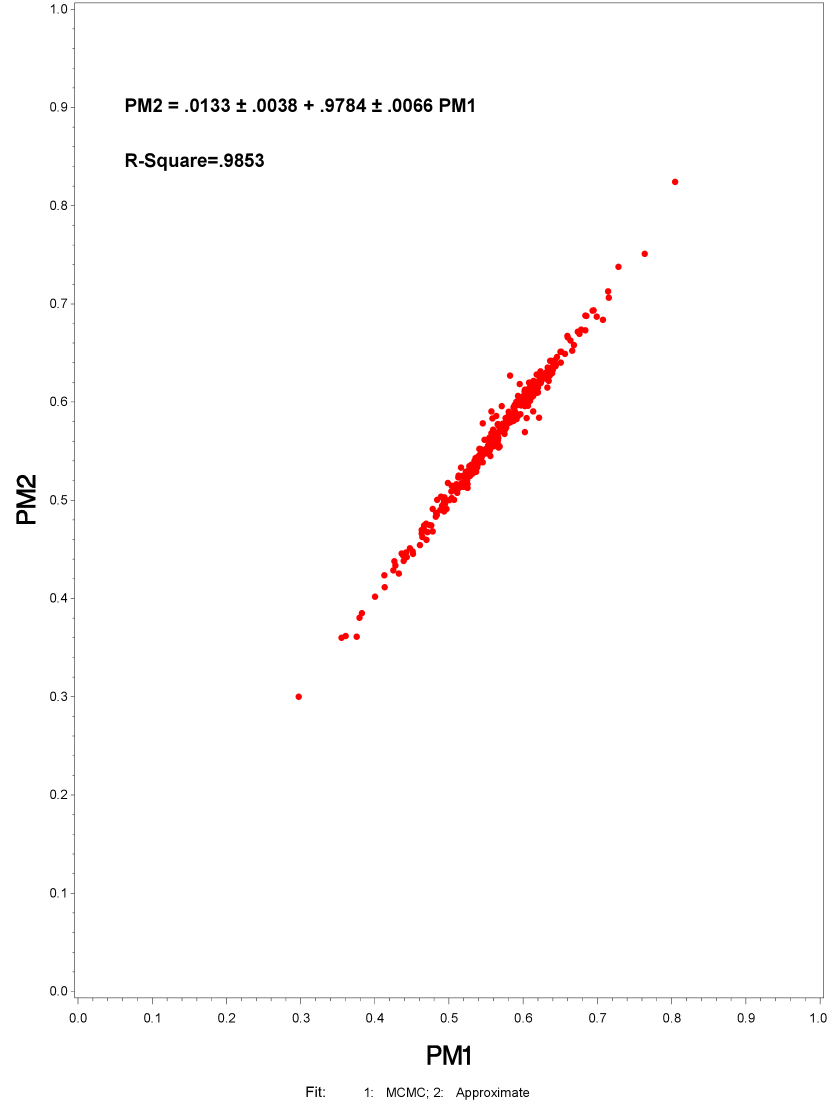
approximation (INNA) and some theoretical results are provided. In Section 3, we present an illustrative
example using the Nepal Living Standards Survey (NLSS II). We compare the approximate method with the
exact method, which is presented in Appendix A. It is worth noting that the word “exact” refers to MCMC without further
approximation. In Section 4, we have discussions and two extensions, both of them can be used to accommodate the NLSS II data
better. Additional technical details are given in the appendices.
2 Approximate Theory and Method
The method we developed here for many small areas can be applied to any generalized linear model in the same manner. Of course, the specific models will be different. For example, for the model for Poisson regression is different from the model for logistic regression. However, note that for logistic regression model, the unit level (binary data, not
binomial counts) are used and for Poisson regression model the count data are collected at an aggregate level.
Our application is on the Nepal Living Standards Survey (NLSS II) and we have binary
data (good health versus poor health) for each individual within a household, and these households are within
wards. Our theory applies to individuals within households or individuals within
wards. We note that the number of members in the , household in the population is and all
household members are sampled, but not all households in a ward are sampled. Our model will hold for all households
but it is convenient to present the model for the sampled households.
Our logistic regression model applies to all population households. We know
how many households are in each ward (sampled or nonsampled) but we do not know how many members are
in each nonsampled household. Let and , denote the responses and the vector of covariates with an intercept ().
A standard hierarchical Bayesian logistic regression model is
|
|
|
|
|
|
|
|
|
Here, , are the random effects and are the regression coefficients with , the variance of the random effects.
For our approximation methods, we will use an equivalent model. It is convenient to separate
into and , where . Omitting the intercept term from the covariate , we
have
|
|
|
|
|
|
|
|
|
(1) |
where essentially we have made the transformation .
The parameters of interest are the household proportions,
|
|
|
(2) |
The give smoothed estimates at the household level and actually predictions
for the nonsample households.
A similar formula can be written down for the wards. Because we are not linking
the census to the NLSS, we do not have the covariates and the number of members in
each nonsampled households, both being obtained using a Bayesian bootstrap (Rubin 1981) of the
original samples.
To develop the approximate methodology, we will work with the no-intercept model. Then, using Bayes’ theorem, the joint posterior density for the parameters is
|
|
|
(3) |
The posterior density in (3) is a non-standard density, and there are difficulties
in fitting it using Markov chain Monte Carlo methods, more so when is large. This
motivates our approximate methods.
We note that given , the are independent with
|
|
|
(4) |
For the nonsampled households, .
More importantly with respect to posterior inference about , the conditional posterior densities for the can be written down easily.
2.1 Approximation to the Posterior Density
In this section we discuss the approximation to the joint posterior density
in (3).
Let denote the density of a vector of parameters
. Let
denote the gradient vector and the Hessian matrix
at some point .
Lemma 2.1.
Let be a logconcave density function with the parameter
.
Then,
approximately has a multivariate normal distribution,
|
|
|
Proof.
Simply applying the second-order multivariate Taylor series of at
, we have
|
|
|
We remark that because of logconcavity, is positive definite. Also because we are not required to find the mode of ,
does not have to be the solution of the gradient vector set to the zero vector. So that the term involving
is a correction to .
∎
Momentarily, we consider a flat prior and the (i.e., fiducial inference). That is,
|
|
|
|
|
|
The joint posterior density is
|
|
|
(5) |
The logarithm of the joint posterior density (or log-likelihood) is
|
|
|
Let . First, we find a
convenient point to expand the log-likelihood in a multivariate Taylor’s series
expansion. In Appendix B, we show how to obtain quasi-modes for and
, of the log-likelihood function.
First, we use the empirical logistic transform to get an estimate of , where
|
|
|
See Appendix C.
Second, obtain the first derivative of log-likelihood of , use a first-order Taylor’s expansion
with replaced by , and set to zero to get
|
|
|
Third, we obtain quasi-modes for the , a refinement of the . We use the log-likelihood of the with
the regression coefficients replaced by , and solve its first derivative for zeros using a first-order
Taylor’s series expansion to get
|
|
|
Let .
Next, we evaluate
and H at the quasi-modes ,
|
|
|
|
|
|
The partial derivatives can be expressed in terms of response and covariates as
|
|
|
|
|
|
|
|
|
|
|
|
|
|
|
For the convenience of computation, denote and where
|
|
|
|
|
|
Note that D is a diagonal matrix.
|
|
|
|
|
|
Lemma 2.2.
Assuming that the design matrix is full-rank and , the posterior density, in (5), is logconcave.
Proof.
If , there are solutions to the gradient vector set
to zero.
Let . Then,
, and of the negative Hessian matrix can be written as,
|
|
|
|
|
|
|
|
|
Clearly, is positive definite. Thus, to show that is positive definite, we show that
its Schur complement of , , is positive definite (e.g., see Boyd
and Vandenberghe 2004). Let . Then, the Schur complement is
|
|
|
It is now easy to show that
|
|
|
Therefore, is positive definite, and is logconcave.
∎
We next establish the first key result presented in Theorem 2.1.
Theorem 2.1.
Assuming that the design matrix is full-rank and , the posterior density, in (5) is approximately
a multivariate normal density, and
|
|
|
where
|
|
|
Proof.
By Lemma 2.2 the posterior density is logconcave. By Lemma 2.1 the posterior density is approximately
a multivariate normal density. We provide the approximate mean and variance to completely specify the
multivariate normal density.
By Lemma 2.1, evaluating all appropriate quantities at , the posterior mean is
|
|
|
Also, by Lemma 1, the posterior variance is
|
|
|
That is, the approximate joint posterior density is
|
|
|
Finally, using a standard property of the multivariate normal density,
it follows that approximately,
|
|
|
∎
2.2 Integrated Nested Normal Approximation
In this section, we obtain the integrated nested normal approximation (INNA).
INNA, which does not require posterior modes, is competitive to the integrated nested
Laplace approximation (INLA) that requires posterior modes.
Next, using the normal priors for the and Theorem 1, we have the following approximate hierarchical Bayesian regression model,
|
|
|
|
|
|
|
|
|
|
|
|
(6) |
where
is a vector of ones.
Then, using Bayes’ theorem again, the approximate joint posterior density for the parameters and is
|
|
|
|
|
|
(7) |
Next, we state the main result of the paper in Theorem 2.2.
Theorem 2.2.
Using the multiplication rule, the joint posterior density,
in (7), can be approximated by
|
|
|
where the three densities on the right-hand side are to be determined.
Proof.
First, it can be shown that
|
|
|
(8) |
which is .
Because is diagonal, given , the are independent. This is an
important result because parallel computation can be done for , which accommodates time-consuming and massive storage challenges in big data analysis. This result holds for the exact conditional posterior density of the
.
Second, because
has a multivariate normal distribution, we can integrate out
from the joint posterior density to get the joint posterior density of
and ,
|
|
|
(9) |
and
|
|
|
(10) |
Let
|
|
|
|
|
|
|
|
|
|
|
|
After extensive algebraic manipulation, we can show that
has an approximate multivariate normal density,
|
|
|
(11) |
which is denoted by .
Third, because the approximate conditional distribution of is a multivariate normal distribution, we can integrate out
from the joint density of in (9) to get the posterior density,
|
|
|
|
|
|
where .
Our INNA method is sampling based and it uses random samples. Samples are obtained by first
drawing from , then and finally
, the first two densities use standard draws, but
the third is a nonstandard density.
Since , we make a transformation to so that . Then,
posterior density, , is
|
|
|
(12) |
The grid method is used to sample .
INNA simply uses the multiplication rule to get samples from the approximate joint posterior density, which is
|
|
|
(13) |
where is given in (4),
is given in (11) and is given in
(12) after re-transformation.
Equation (13) is the basis of our INNA approximation. This is simply the multiplication rule of probability;
simply draw from (12) and retransform to to get ,
draw
from (multivariate normal and
from
. Use a Metropolis algorithm with an approximate normal proposal density to draw samples of independently given
, and data. We run each Metropolis 100 times and picked the last one.
If the Metropolis step fails (jumping rate is not in , we use a grid method instead. Parallel computing can also be used in this latter step. This is performed in the same manner for the exact method. For our application with 3,912 households, this latter step runs very fast. Of course, with much larger number of households, the computing time will be substantial, but now parallel
computing is available.
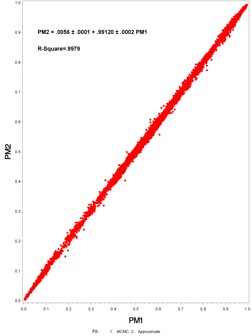
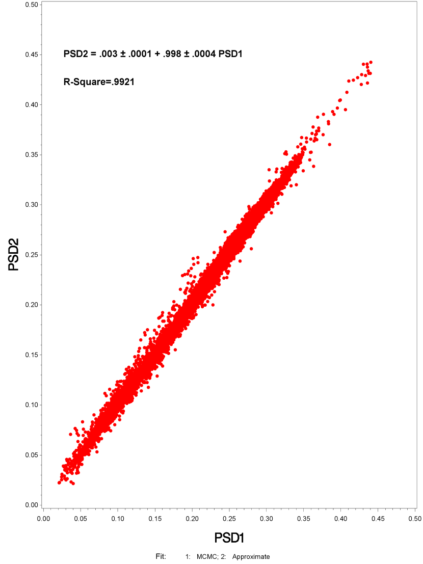
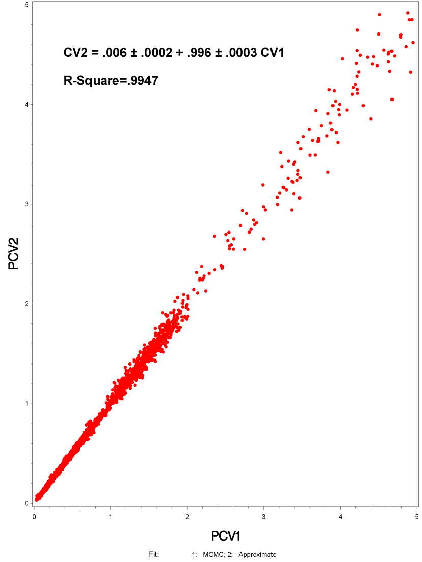
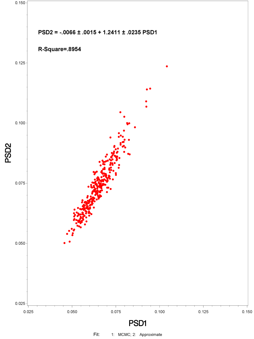
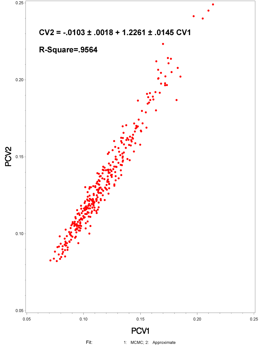
2.3 Comparison of the Two Methods
As a summary, we compare the approximate and exact methods. The exact method is given in Appendix A.
First, we note that the exact method actually uses the approximate method. We
use a Metropolis step with , obtained from the approximate method.
We fit a multivariate Student’s distribution with degrees of freedom to the iterates,
from the approximate method as the proposal density in the Metropolis step. It is standard to tune the Metropolis step
by varying .
We present two differences between the two methods. First, both methods are sampling based; the approximate method
implements random samples and the exact method a Markov chain.
Second, is used for the approximate method
and a Metropolis step is used for .
It is this Metropolis step that is time-consuming (20 minutes versus 20 seconds); for a million households, we
can prorate this time (80 hours versus 80 minutes), enormous savings.
We present three similarities between the two methods.
First, , are drawn
the same way using a Metropolis step with proposal density .
Grids are used when the Metropolis step fails. Parallel computing can be done easily in both cases.
Second, for , are normal densities
(). Third, for prediction two Bayesian bootstraps are used to get the nonsampled household
sizes and the nonsampled covariates ( two million people). This is done within wards.
4 Concluding Remarks
We make three statistical comments.
First, the approximate method is necessary when there are a large number (millions) of households (clusters or areas).
Second, it is difficult to use the census data effectively but it is desirable (matching problem). Third,
it is possible to obtain similar approximations for spatial priors and Dirichlet process priors (under investigation)
We make four computational comments. First, parallel computing is needed for big data (numerous small areas).
Second, consensus Monte Carlo method, although problematic, is needed for large data (storage problems).
For the NLSS survey, stratification already exists; Nepal has six strata and our INNA procedure can be applied in
each stratum in parallel. Third, MCMC (not INLA) methods are useful for small datasets; good approximations are needed
for large datasets (big data). Finally, INNA is potentially useful because modes are not required (INLA needs modes).
We mention two possible extensions. The first extension is about survey weights. The second extension
is to a sub-area model.
PPS sampling is used in the first-stage of the survey design. Thus, there are survey weights (design, not adjusted
weights). All households (each member) in a psu has the same weight. So we can proceed in one of the two ways in our
analysis. First, we can use an adjusted logistic likelihood incorporating the survey weights. We discuss a single area,
then we show how to extend it to small area problems. Let , denote the survey weights for
sampling from a single area. Let
|
|
|
see Potthof, Woodbury and Manton (1992) for pioneering work on equivalent sample sizes.
For , we have
|
|
|
|
|
|
|
|
|
For small areas, with
, we have
|
|
|
|
|
|
Our second extension is to sub-area model. One example already discussed in the literature
is that of Torabi and Rao (2014), who extended the Fay-Herriot model (Fay and Herriot 1979), not for logistic
regression. For our problem, the areas are the wards and sub-areas are the households.
Let , denote the areas and , denote the sub-areas.
We assume that
|
|
|
|
|
|
|
|
|
|
|
|
For logistic regression, this research is currently in progress.
Appendix A Exact Method for Logistic Regression
Recall the Bayesian logistic model with covariates that we worked on with INNA method
|
|
|
|
|
|
|
|
|
(A.1) |
According to Bayes’ theorem, the joint posterior density of the parameters is
|
|
|
|
|
|
Theorem A.1.
The joint posterior density, , is proper provided
that the design matrix is full rank and .
Proof.
With a flat prior on the and
, the same argument as in Lemma 2.2 gives
logconcavity of the joint posterior density. Putting a logconcave prior on the does
not change the logconavity of because the product
of two logconcave densities is another logconcave density. In addition, logconcave densities
have sub-exponential tails and their moment generating functions exist (see Dharmadhikari and Joag-Dev 1988). That is,
finite for all . Therefore, as
long as is proper as for . So that,
is proper.
∎
The standard MCMC logistic regression exact method is complicated to work with and it takes longer time to get posterior samples. We apply Metropolis Hastings sampler to draw samples for parameters
, and
.
The idea of exact method is to get full conditional posterior distributions for all of the parameters in the model, and then get a large number of independent samples of each parameter with its full conditional posterior density.
First, we integrate
from the posterior density to get the joint posterior density of as
|
|
|
|
|
|
Notice that this is not a simple distribution function for the integration, so we apply numerical integration. Divide the integration domain to equal intervals . Let with standard normal distribution. We get an approximate density (very accurate though),
|
|
|
|
|
|
Take the middle point of each interval to estimate the cumulative density function, and denote . We have the following deduction
|
|
|
The integration is now over a standard normal distribution. We consider the interval (-3, 3) for numerical integration, since this domain (standard normal) covers 99.74% of the distribution that we are dealing with. We take m=100 grid points. Then the joint posterior density for
and can be expressed as
|
|
|
(A.2) |
We use the Metropolis sampler to draw samples from the joint posterior density of drawing
and simultaneously. We use
the transformation . We obtain a proposal density for
using a multivariate Student’s density as follows. First, when we run the approximate method, we
obtain the approximate mean,
and covariance matrix
of
. So we take .
Tuning of the Metropolis sampler is obtained by varying (e.g., corresponds to approximately a logistic
random vector). We run the Metropolis sampler in a nonstandard manner, as the Markov chain runs, we reserve
those iterates when the algorithm moves. In this way while tuning, is required to get a reasonable jumping rate,
no other diagnostics (autocorrelation, effective sample size, test of stationarity, thinning) are needed.
The number of nonsampled households in the sampled PSUs are known, but the number of members of a nonsampled household
and their covariates are unknown. For each sampled PSU, we obtain the empirical distribution of the number
of members and their covariates. Then, we use two Bayesian bootstraps to sample the number of members and their
covariates from the pool of the PSU. For both bootstraps we use samples.
Appendix B Quasi-Modes for Logistic Regression
Now we have to specify , ,
and . Consider the log likelihood function
|
|
|
|
|
|
(B.1) |
As an estimate of , we use the empirical logistic transform ,
|
|
|
See Appendix C.
Plug in the log likelihood function (B.1) and consider it as a function of only,
|
|
|
The first derivative function of over is
|
|
|
|
|
|
(B.2) |
Typically, we can solve the equation for the mode as the maximum likelihood estimator (MLE), but here it is not easy to solve the equation because is complex. We use first order Taylor series approximation to simplify the above function. Since the first order Taylor expansion of equals , (B.2) equals to
|
|
|
(B.3) |
This is still complex. We apply Taylor series again and get expansion of the term to the first order as . Thus (B.3) approximately equals
|
|
|
|
|
|
(B.4) |
(B.4) is easy to solve. Solve for , and we can get the approximate posterior mode of
|
|
|
(B.5) |
Plug in the likelihood function (B.1) and consider it as a function of
only,
|
|
|
The first derivative function of over is
|
|
|
(B.6) |
Similar to above, we apply Taylor series approximation
|
|
|
So (B.6) equals
|
|
|
Solve for , then the approximate posterior mode (quasi-mode) of can be obtained as
|
|
|
Notice that the term in denominator may cause trouble for this posterior mode, because the binary response variable could lead to for some , so that . We borrow the idea from the empirical logistic transform (ELT) and make a little adjustment to avoid 0’s in denominator
|
|
|
(B.7) |
Appendix C Empirical Logistic Transform (ELT)
We consider the empirical logistic transform (ELT) without covariates for binary
data. See Cox and Snell (1972) for the empirical logistic transform (ELT) that
accommodates binary data.
Letting denote a binomial random variable with success probability , the empirical logistic transform, , is
|
|
|
and the corresponding variance V is
|
|
|
Then, using the approximation of Cox and Snell (1972),
has a normal distribution with mean and variance V, where is unknown according to Cox and Snell (1972).
Suppose
is the variable of length . Each of the binary response follows a binomial distribution with corresponding number of observations and probability . The goal is to estimate the Bernoulli probability parameter . Here we assume that
|
|
|
and for logistic transform we
define as the the empirical logistic transforms, and as the associated variances. Then,
|
|
|
We can actually start with this approximation based on the empirical logistic transform. However, this approximation
will not work for binary data with covariates at the unit level, but we will make use it in our approximation for
logistic regression with binary data in a less important manner.