Table Space Designs For Implicit and Explicit Concurrent Tabled Evaluation

Abstract

One of the main advantages of Prolog is its potential for the implicit exploitation of parallelism and, as a high-level language, Prolog is also often used as a means to explicitly control concurrent tasks. Tabling is a powerful implementation technique that overcomes some limitations of traditional Prolog systems in dealing with recursion and redundant sub-computations. Given these advantages, the question that arises is if tabling has also the potential for the exploitation of concurrency/parallelism. On one hand, tabling still exploits a search space as traditional Prolog but, on the other hand, the concurrent model of tabling is necessarily far more complex since it also introduces concurrency on the access to the tables. In this paper, we summarize Yap’s main contributions to concurrent tabled evaluation and we describe the design and implementation challenges of several alternative table space designs for implicit and explicit concurrent tabled evaluation which represent different trade-offs between concurrency and memory usage. We also motivate for the advantages of using fixed-size and lock-free data structures, elaborate on the key role that the engine’s memory allocator plays on such environments, and discuss how Yap’s mode-directed tabling support can be extended to concurrent evaluation. Finally, we present our future perspectives towards an efficient and novel concurrent framework which integrates both implicit and explicit concurrent tabled evaluation in a single Prolog engine. Under consideration in Theory and Practice of Logic Programming (TPLP).

1 Introduction

Tabling [Chen and Warren (1996)] is a recognized and powerful implementation technique that overcomes some limitations of traditional Prolog systems in dealing with recursion and redundant sub-computations. Tabling is a refinement of SLD resolution that stems from one simple idea: save intermediate answers from past computations so that they can be reused when a similar call appears during the resolution process. Tabling based models are able to reduce the search space, avoid looping, and always terminate for programs with the bounded term-size property [Chen and Warren (1996)].

Tabling has become a popular and successful technique thanks to the ground-breaking work in the XSB Prolog system and in particular in the SLG-WAM engine [Sagonas and Swift (1998)], the most successful engine of XSB. The success of SLG-WAM led to several alternative implementations that differ in the execution rule, in the data-structures used to implement tabling, and in the changes to the underlying Prolog engine. Currently, the tabling technique is widely available in systems like XSB Prolog [Swift and Warren (2012)], Yap Prolog [Santos Costa et al. (2012)], B-Prolog [Zhou (2012)], ALS Prolog [Guo and Gupta (2001)], Mercury [Somogyi and Sagonas (2006)], Ciao Prolog [Chico et al. (2008)] and more recently in SWI Prolog [Desouter et al. (2015)] and Picat [Zhou et al. (2015)].

One of the main advantages of Prolog is its potential for the implicit exploitation of parallelism. Many sophisticated and well-engineered parallel Prolog systems exist in the literature [Gupta et al. (2001)], being the most successful those that exploit implicit or-parallelism [Lusk et al. (1988), Ali and Karlsson (1990), Gupta and Pontelli (1999)], implicit and-parallelism [Hermenegildo and Greene (1991), Shen (1992), Pontelli and Gupta (1997)] or a combination of both [Santos Costa et al. (1991)]. Or-parallelism arises when more than one clause unifies with the current call and it corresponds to the simultaneous execution of the body of those different clauses. And-parallelism arises when more than one subgoal occurs in the body of the clause and it corresponds to the simultaneous execution of the subgoals contained in a clause’s body.

On the other hand, as a high-level language, Prolog is also often used as a means to explicitly control and schedule concurrent tasks [Carro and Hermenegildo (1999), Fonseca et al. (2009)]. The ISO Prolog multithreading standardization proposal [Moura (2008)] is currently implemented in several Prolog systems including XSB, Yap, Ciao and SWI, providing a highly portable solution given the number of operating systems supported by these systems. In a nutshell, multithreading in Prolog is the ability to concurrently perform multiple computations, in which each computation runs independently but shares the database (clauses). It is therefore unsurprising that implicit and explicit concurrent/parallel evaluation has been an important subject in the design and development of Prolog systems.

Nowadays, the increasing availability of computing systems with multiple cores sharing the main memory is already a standardized, high-performance and viable alternative to the traditional (and often expensive) shared memory architectures. The number of cores per processor is expected to continue to increase, further expanding the potential for taking advantage of such support as an increasingly popular way to implement dynamic, highly asynchronous, concurrent and parallel programs.

Besides the two traditional approaches to concurrency/parallelism: (i) fully implicit, i.e., it is left to the runtime system to automatically detect the potential concurrent tasks in the program, assign them for parallel execution and control and synchronize their execution; and (ii) fully explicit, i.e., it is left to the user to annotate the tasks for concurrent execution, assign them to the available workers and control the execution and the synchronization points, the recent years have seen a lot of proposals trying to combine both approaches in such a way that the user relies on high-level explicit parallel constructs to trigger parallel execution and then it is left to the runtime system the control of the low-level execution details. In the combined approach, in general, a program begins as a single worker that executes sequentially until reaching a parallel construct. When reaching a parallel construct, the runtime system launches a set of additional workers to exploit concurrently the sub-computation at hand. Concurrent execution is then handled implicitly by the execution model taking into account additional directive restrictions given to the parallel construct.

Multiple examples of frameworks exist that follow the combined approach. For example, for imperative programming languages, the OpenMP [Chapman et al. (2008)], Intel Threading Building Blocks [Reinders (2007)] and Cilk [Blumofe et al. (1995)] frameworks provide runtime systems for multithreaded parallel programming, providing users with the means to create, synchronize, and schedule threads efficiently. For functional programming languages, the Eden [Loogen et al. (2005)] and HDC [Herrmann and Lengauer (2000)] Haskell based frameworks allow the users to express their programs using polymorphic higher-order functions. For object-oriented programming languages, MALLBA [Alba et al. (2002)] and DPSKEL [Peláez et al. (2007)] frameworks also showed relevant speedups in the parallel evaluation of combinatorial optimization benchmarks.

In the specific case of Prolog, given the advantages of tabled evaluation, the question that arises is if a tabling mechanism has the potential for the exploitation of concurrency/parallelism. On one hand, tabling still exploits a search space as traditional Prolog, but on the other hand, the concurrent model of tabling is necessarily far more complex than the traditional concurrent models, since it also introduces concurrency on the access to the tables. In a concurrent tabling system, tables may be either private or shared between workers. On one hand, private tables can be easier to implement but restrict the degree of concurrency. On the other hand, shared tables have all the associated issues of locking, synchronization and potential deadlocks. Here, the problem is even more complex because we need to ensure the correctness and completeness of the answers found and stored in the shared tables. Thus, despite the availability of both threads and tabling in Prolog compilers such as XSB, Yap, Ciao and SWI, the implementation of these two features such that they work together seamlessly implies complex ties to one another and to the underlying engine.

To the best of our knowledge, only the XSB and Yap systems support the combination of tabling with some form of concurrency/parallelism. In XSB, the SLG-WAM execution model was extended with a shared tables design [Marques and Swift (2008)] to support explicit concurrent tabled evaluation using threads. It uses a semi-naive approach that, when a set of subgoals computed by different threads is mutually dependent, then a usurpation operation synchronizes threads and a single thread assumes the computation of all subgoals, turning the remaining threads into consumer threads. The design ensures the correct execution of concurrent sub-computations but the experimental results showed some limitations [Marques et al. (2010)]. Yap implements both implicit and explicit concurrent tabled evaluation, but separately. The OPTYap design [Rocha et al. (2005)] combines the tabling-based SLG-WAM execution model with implicit or-parallelism using shared memory processes. More recently, a second design supports explicit concurrent tabled evaluation using threads [Areias and Rocha (2012b)], but using an alternative view to XSB’s design. In Yap’s design, each thread has its own tables, i.e., from a thread point of view the tables are private, but at the engine level it uses a common table space, i.e., from the implementation point of view the tables are shared among threads.

In this paper, we summarize Yap’s main developments and contributions to concurrent tabled evaluation and we describe the design and implementation challenges of several alternative table space designs for implicit and explicit concurrent tabled evaluation which represent different trade-offs between concurrency and memory usage. We also motivate for the advantages of using fixed-size and lock-free data structures for concurrent tabling and we elaborate on the key role that the engine’s memory allocator plays on such an environment where a higher number of simultaneous memory requests for data structures in the table space can be made by multiple workers. We also discuss how Yap’s mode-directed tabling support [Santos and Rocha (2013)] can be extended to concurrent evaluation. Mode-directed tabling is an extension to the tabling technique that allows the aggregation of answers by specifying pre-defined modes such as min or max. Mode-directed tabling can be viewed as a natural tool to implement dynamic programming problems, where a general recursive strategy divides a problem in simple sub-problems whose goal is, usually, to dynamically calculate optimal or selective answers as new results arrive.

Finally, we present our future perspectives towards an efficient and novel concurrent framework which integrates both implicit and explicit concurrent tabled evaluations in a single tabling engine. This is a very complex task since we need to combine the explicit control required to launch, assign and schedule tasks to workers, with the built-in mechanisms for handling tabling and/or implicit concurrency, which cannot be controlled by the user. Such a framework could renew the glamour of Prolog systems, especially in the concurrent/parallel programming community. Combining the inherent implicit parallelism of Prolog with explicit high-level parallel constructs will clearly enhance the expressiveness and the declarative style of tabling, and simplify concurrent programming.

In summary, the main contributions of this paper are: (i) a systematic presentation of the different alternative table space designs implemented in Yap for implicit and explicit concurrent tabled evaluation (which were dispersed by several publications); (ii) a formalization of the total memory usage of each table space design, which allows for a more rigorous comparison and demonstrates how each design is dependent on the number of workers and on the number of tabled calls in evaluation; (iii) a performance analysis of Yap’s tabling engine highlighting how independent concurrent flows of execution interfere at the low-level engine and how dynamic programming problems fit well with concurrent tabled evaluation; and (iv) the authors’ perspectives towards a future concurrent framework which integrates both implicit and explicit concurrent tabled evaluations in a single tabling engine.

The remainder of the paper is organized as follows. First, we introduce some basic concepts and relevant background. Then, we present the alternative table space designs for implicit and explicit concurrent tabled evaluation. Next, we discuss the most important engine components and implementation challenges to support concurrent tabled evaluation and we show a performance analysis of Yap’s tabling engine when using different table space designs. At last, we discuss future perspectives and challenging research directions.

2 Background

This section introduces relevant background needed for the following sections. It briefly describes Yap’s original table space organization and presents Yap’s approach for supporting mode-directed tabling.

2.1 Table Space Organization

The basic idea behind tabling is straightforward: programs are evaluated by saving intermediate answers for tabled subgoals so that they can be reused when a similar call appears during the resolution process. First calls to tabled subgoals are considered generators and are evaluated as usual, using SLD resolution, but their answers are stored in a global data space, called the table space. Similar calls are called consumers and are resolved by consuming the answers already stored for the corresponding generator, instead of re-evaluating them against the program clauses. During this process, as further new answers are found, they are stored in their table entries and later returned to all similar calls.

Call similarity thus determines if a subgoal will produce their own answers or if it will consume answers from a generator call. There are two main approaches to determine if a subgoal $A$ is similar to a subgoal $B$:

• Variant-based tabling [Ramakrishnan et al. (1999)]: $A$ and $B$ are variants if they can be identical through variable renaming. For example, $p(X,1,Y)$ and $p(W,1,Z)$ are variants because both can be renamed into $p(VAR_{0},1,VAR_{1})$.

• Subsumption-based tabling [Rao et al. (1996)]: subgoal $A$ is considered similar to $B$ if $A$ is subsumed by $B$ (or $B$ subsumes $A$), i.e., if $A$ is more specific than $B$ (or an instance of). For example, subgoal $p(X,1,2)$ is subsumed by subgoal $p(Y,1,Z)$ because there is a substitution $\{Y=X,Z=2\}$ that makes $p(X,1,2)$ an instance of $p(Y,1,Z)$.

Variant-based tabling has been researched first and is arguably better understood. For some types of programs, subsumption-based tabling yields superior time performance [Rao et al. (1996), Johnson et al. (1999)], as it allows greater reuse of answers, and better space usage, since the answer sets for the subsumed subgoals are not stored. However, the mechanisms to efficiently support subsumption-based tabling are harder to implement, which makes subsumption-based tabling not as popular as variant-based tabling. The Yap Prolog system implements both approaches for sequential tabling [Santos Costa et al. (2012), Cruz and Rocha (2010)], but for concurrent tabled evaluation, Yap follows the variant-based tabling approach.

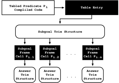
Figure 1: Yap’s original table space organization

A critical component in the implementation of an efficient tabling system is thus the design of the data structures and algorithms to access and manipulate the table space. Yap uses trie data structures to implement efficiently the table space [Ramakrishnan et al. (1999)]. Tries are trees in which common prefixes are represented only once. The trie data structure provides complete discrimination for terms and permits lookup and possible insertion to be performed in a single pass through a term, hence resulting in a very efficient and compact data structure for term representation.

Figure 1 shows the original table space organization for a tabled predicate $P_{i}$ in Yap. At the entry point, we have the table entry data structure. This structure stores common information for the tabled predicate, such as the predicate’s arity or the predicate’s evaluation strategy, and it is allocated when the predicate is being compiled, so that a pointer to the table entry can be included in its compiled code. This guarantees that further calls to the predicate will access the table space starting from the same point. Below the table entry, we have the subgoal trie structure. Each different tabled subgoal call $P_{i.j}$ to the predicate corresponds to a unique path through the subgoal trie structure, always starting from the table entry, passing by several subgoal trie data units, the subgoal trie nodes, and reaching a leaf data structure, the subgoal frame. The subgoal frame stores additional information about the subgoal and acts like an entry point to the answer trie structure. Each unique path through the answer trie data units, the answer trie nodes, corresponds to a different tabled answer to the entry subgoal.

2.2 Mode-Directed Tabling and Dynamic Programming

The tabling technique can be viewed as a natural tool to implement dynamic programming problems. Dynamic programming is a general recursive strategy that consists in dividing a problem in simple sub-problems that, often, are the same. Tabling is thus suitable to use with this kind of problems since, by storing and reusing intermediate results while the program is executing, it avoids performing the same computation several times.

In a traditional tabling system, all arguments of a tabled subgoal call are considered when storing answers into the table space. When a new answer is not a variant of any answer that is already in the table space, then it is always considered for insertion. Therefore, traditional tabling is very good for problems that require storing all answers. However, with dynamic programming, usually, the goal is to dynamically calculate optimal or selective answers as new results arrive. Solving dynamic programming problems can thus be a difficult task without further support.

Mode-directed tabling is an extension to the tabling technique that supports the definition of modes for specifying how answers are inserted into the table space. Within mode-directed tabling, tabled predicates are declared using statements of the form ‘$table~{}p(m_{1},...,m_{n})$’, where the $m_{i}$’s are mode operators for the arguments. The idea is to define the arguments to be considered for variant checking (the index arguments) and how variant answers should be tabled regarding the remaining arguments (the output arguments). In Yap, index arguments are represented with mode index, while arguments with modes first, last, min, max, sum and all represent output arguments [Santos and Rocha (2013)]. After an answer is generated, the system tables the answer only if it is preferable, accordingly to the meaning of the output arguments, than some existing variant answer.

In Yap, mode-directed tabled predicates are compiled by extending the table entry data structure to include a mode array, where the information about the modes is stored, and by extending the subgoal frames to include a substitution array, where the mode information is stored together with the number of free variables associated with each argument in the subgoal call [Santos and Rocha (2013)]. When a new answer is found, it must be compared against the answer(s) already stored in the table, accordingly to the modes defined for the corresponding arguments. If the new answer is preferable, the old answer(s) must be invalidated and the new one inserted in the table. The invalidation process consists in: (a) deleting all intermediate answer trie nodes corresponding to the answers being invalidated; and (b) tagging the leaf nodes of such answers as invalid nodes. Invalid nodes are only deleted when the table is later completed or abolished.

Regarding the table space designs that we present next, the support for mode-directed tabling is straightforward when the table data structures are not accessed concurrently for write operations. The problem arises for the designs which do not require the completion of tables to share answers, since we need to efficiently support concurrent delete operations on the trie structures and correctly handle the interface between consumer calls and the navigation in the answer tries.

3 Concurrent Table Space Designs

This section presents alternative table space designs for implicit and explicit concurrent tabled evaluation, which represent different trade-offs between concurrency and memory usage.

3.1 Implicit versus Explicit Concurrent Tabled Evaluation

Remember the two traditional approaches to concurrency/parallelism: fully implicit and fully explicit. With fully implicit, it is left to the runtime system to automatically detect the potential concurrent tasks in the program, assign them for concurrent/parallel execution and control and synchronize their execution. In such approach, the running workers (processes, threads or both) often share the data structures representing the data of the problem since tasks do not need to be pre-assigned to workers as any worker can be scheduled to perform an unexplored concurrent task of the problem. For tabling, that means that the table space data structures must be fully shared among all workers. This is the case of the OPTYap design [Rocha et al. (2005)], which combines the tabling-based SLG-WAM execution model with implicit or-parallelism using shared memory processes.

On the other hand, with a fully explicit approach, it is left to the user to annotate the tasks for concurrent execution, assign them to the available workers and control the execution and the synchronization points. In such approach, the running workers often execute independently a well-defined (set of) task(s). For tabling, that means that each evaluation only depends on the computations being performed by the worker itself, i.e., a worker does not need to consume answers from other workers’ tables as it can always be the generator for all of its subgoal calls. These are the cases of XSB [Marques and Swift (2008)] and Yap [Areias and Rocha (2012b)] designs which support explicit concurrent tabled evaluation using threads. In any case, the table space data structures can be either private or partially shared between workers. Yap proposes several alternative designs to implement the table space for explicit concurrent tabled evaluation. Table 1 overviews the several Yap’s table space designs and how they differ in the way the internal table data structures are implemented and accessed. In the following subsections, we present the several designs and we show a detailed analysis of the memory usage of each.

Table 1: Yap’s table space designs – Cooperative Sharing (CS), No-Sharing (NS), Subgoal-Sharing (SS), Full-Sharing (FS), Partial Answer Sharing (PAS) and Private Answer Chaining (PAC) – and the implementation and access of the data structures in each design: as private data structures (–); as fully shared data structures (F); as partially shared data structures (P); and as data structures with concurrent read (r) and concurrent write (w) operations.

Data	Implicit	Explicit
Structure	CS	NS	SS	FS	PAS	PAC
Table Entry	$F(r)$	$F(r)$	$F(r)$	$F(r)$	$F(r)$	$F(r)$
Subgoal Trie	$F(rw)$	–	$F(rw)$	$F(rw)$	$F(rw)$	$F(rw)$
Subgoal Frame	$F(rw)$	–	–	$P(rw)$	$P(r)$	$P(rw)$
Answer Trie	$F(rw)$	–	–	$F(rw)$	$P(r)$	$P(rw)$

3.2 Cooperative Sharing Design

The Cooperative Sharing (CS) design supports the combination of tabling with implicit or-parallelism using shared memory processes [Rocha et al. (2005)]. The CS design was the first concurrent table space design implemented in Yap Prolog. It follows Yap’s original table space organization, as shown in Fig. 1, and extends it with some sort of synchronization mechanisms to deal with concurrent accesses. In what follows, we will not consider synchronization mechanisms which require extending the table space data structures with extra fields, like lock fields, since several synchronization techniques exist that do not require an actual lock field. Two examples are: (i) the usage of an external global array of locks; or (ii) the usage of low level Compare-And-Swap (CAS) operations. We discuss this in more detail in section 4.

Remember from Fig. 1 that, at the entry point, we have a table entry ($TE$) data structure for each tabled predicate $P_{i}$. Underneath each $TE$, we have a subgoal trie ($ST(P_{i})$) and several subgoal frame ($SF$) data structures for each tabled subgoal call $P_{i.j}$ made to the predicate. Finally, underneath each $SF$, we have an answer trie ($AT(P_{i.j})$) structure with the answers for the corresponding subgoal call $P_{i.j}$. Please note that the size of the $TE$ and $SF$ data structures is fixed and independent from the predicate, but the size of the $ST(P_{i})$ and $AT(P_{i.j})$ data structures varies accordingly to the number of subgoal calls made and answers found during tabled evaluation.

We can now formalize the Total Memory Usage (TMU) of the CS design. For this, we assume that all tabled predicates are completely evaluated, meaning that the engine will not allocate any further data structures on the table space. Given $NP$ tabled predicates, Eq. 1 presents the $TMU$ of the CS design ($TMU_{CS}$).

$$TMU_{CS}=\sum\limits_{i=1}^{NP}MU_{CS}(P_{i})$$ (1)

$$where~{}~{}MU_{CS}(P_{i})=TE+ST(P_{i})+\sum\limits^{NC(P_{i})}_{j=1}[SF+AT(P_{i.j})]$$

The $TMU_{CS}$ is given by the summation of the Memory Usage (MU) of each predicate $P_{i}$, i.e, the $MU_{CS}(P_{i})$ values, which correspond then to the sum of each structure inside the table space for the corresponding predicate $P_{i}$. The $TE$, $ST(P_{i})$, $SF$ and $AT(P_{i.j})$ values represent the amount of the memory used by predicate $P_{i}$ in its table entry, subgoal trie, subgoal frames and answer trie structures, respectively, and the $NC(P_{i})$ value represents the number of diferent tabled subgoal calls made to the predicate. For example, in Fig. 1, the value of $NC(P_{i})$ is $n$.

As a final remark, please note that the total memory usage of the CS design ($TMU_{CS}$) is the same as the total memory usage of Yap’s original table space organization ($TMU_{ORIG}$). Thus, in what follows, we will use the $TE$, $ST(P_{i})$, $SF$ and $AT(P_{i.j})$ values as the reference values for comparison against the other concurrent table space designs.

3.3 No-Sharing Design

Yap implements explicit concurrent tabled evaluation using threads in which each thread’s computation only depends on the evaluations being performed by the thread itself. The No-Sharing (NS) design was the starting design for supporting explicit concurrent tabled evaluation in Yap [Areias and Rocha (2012b)]. In the NS design, each thread allocates fully private tables for each new tabled subgoal being called. In this design, only the $TE$ structure is shared among threads. Figure 2 shows the configuration of the table space for the NS design. For the sake of simplicity, the figure only shows the configuration for a particular predicate $P_{i}$ and a particular subgoal call $P_{i.j}$.

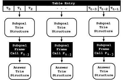
Figure 2: Table space organization for the NS design

The table entry still stores the common information for the predicate but it is extended with a bucket array ($BA$), where each thread $T_{k}$ has its own entry, which then points to the private $ST(P_{i})$, $SF$ and $AT(P_{i.j})$ data structures of the thread. Each bucket array contains as much entry cells as the maximum number of threads that can be created in Yap (currently, Yap supports 1024 simultaneous threads). However, in practice, this solution can be highly inefficient and memory consuming, as this huge bucket array must be always allocated even when only one thread will use it. To solve this problem, we introduce a kind of inode pointer structure, where the bucket array is split into direct bucket cells and indirect bucket cells [Areias and Rocha (2012b)]. The direct bucket cells are used as before, but the indirect bucket cells are allocated only as needed, which alleviates the memory problem and easily adjusts to a higher maximum number of threads. This direct/indirect organization is applied to all bucket arrays.

Since the $ST(P_{i})$, $SF$ and $AT(P_{i.j})$ data structures are private to each thread, they can be removed when the thread finishes execution. Only the table entry is shared among threads. As this structure is created by the main thread when a program is being compiled, no concurrent writing operations will exist between threads and thus no synchronization points are required for the NS design.

Given an arbitrary number of $NT$ running threads and assuming that all threads have completely evaluated the same number $NC(P_{i})$ of tabled subgoal calls, Eq. 2 shows the memory usage for a predicate $P_{i}$ in the NS design ($MU_{NS}(P_{i})$).

$$MU_{NS}(P_{i})=TE_{NS}+NT*[ST(P_{i})+\sum\limits^{NC(P_{i})}_{j=1}[SF+AT(P_{i.j})]]$$ (2)

$$where~{}~{}TE_{NS}=TE+BA$$

The $MU_{NS}(P_{i})$ value is given by the sum of the memory size of the extended table entry structure ($TE_{NS}$) plus the sum of the sizes of the private structures of each thread multiplied by the $NT$ threads. The memory size of $TE_{NS}$ is given by the size of the original $TE$ structure added with the memory size of the bucket array ($BA$). The memory size of the remaining structures is the same as in Yap’s original table space organization.

As for Eq. 1, the total memory usage of the NS design ($TMU_{NS}$) (not shown in Eq. 2) is given by the summation of the memory usage of each predicate, i.e, the $MU_{NS}(P_{i})$ values. Comparing $TMU_{NS}$ with $TMU_{ORIG}$ given $NP$ tabled predicates, the extra memory cost of the NS design to support concurrency is given by the formula:

$$\sum^{NP}_{i=1}[BA+[NT-1]*[ST(P_{i})+\sum\limits^{NC(P_{i})}_{j=1}[SF+AT(P_{i.j})]]]$$

The formula shows that for the base case of 1 thread ($NT=1$), the amount of extra memory spent by the NS design, given by $NP*BA$, corresponds to the bucket array extensions. When increasing the number of threads, the amount of extra memory spent in the $ST(P_{i})$, $SF$ and $AT(P_{i.j})$ data structures increases proportionally to $NT$. This dependency on the number of threads motivated us to create alternative designs that could decrease the amount of extra memory to be spent. The following subsections present such alternative designs.

3.4 Subgoal-Sharing Design

In the Subgoal-Sharing (SS) design, the threads share part of the table space. Figure 3 shows the configuration of the table space for the SS design. Again, for the sake of simplicity, the figure only shows the configuration for a particular tabled predicate $P_{i}$ and a particular subgoal call $P_{i.j}$.

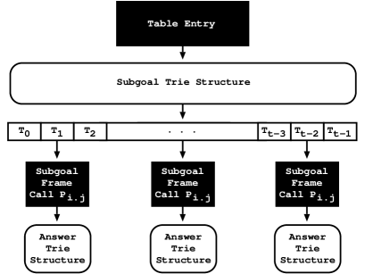
Figure 3: Table space organization for the SS design

In the SS design, the $ST(P_{i})$ data structures are now shared among the threads and the leaf data structure in each subgoal trie path, instead of referring a $SF$ as before, it now points to a $BA$. Each thread $T_{K}$ has its own entry inside the $BA$ which then points to private $SF$ and $AT(P_{i.j})$ structures. In this design, concurrency among threads is restricted to the allocation of trie nodes on the $ST(P_{i})$ structures. Whenever a thread finishes execution, its private structures are removed, but the shared part remains present as it can be in use or be further used by other threads.

Given an arbitrary number of $NT$ running threads and assuming that all threads have completely evaluated the same number $NC(P_{i})$ of tabled subgoal calls, Eq. 3 shows the memory usage for a predicate $P_{i}$ in the SS design ($MU_{SS}(P_{i})$).

The memory usage for the SS design is given by the sum of the memory size of the $TE$ and $ST(P_{i})$ data structures plus the summation, for each subgoal call, of the memory used by the $BA$ added with the sizes of the private structures of each thread multiplied by the $NT$ threads. The memory size of each particular data structure is the same as in Yap’s original table space organization.

$$MU_{SS}(P_{i})=TE+ST(P_{i})+\sum\limits^{NC(P_{i})}_{j=1}[BA+NT*[SF+AT(P_{i.j})]]$$ (3)

Theorem 1 shows the conditions where the SS design uses less memory than the NS design for an arbitrary number of threads $NT$ and an arbitrary number of subgoal calls $NC(P_{i})$.

Theorem 1

If $NT\geq 1$ and $NC(P_{i})\geq 1$ then $MU_{SS}(P_{i})\leq MU_{NS}(P_{i})$ if and only if the formula $[NC(P_{i})-1]*BA\leq[NT-1]*ST(P_{i})$ holds.

Theorem 1 shows that the comparison between the NS and SS designs depends directly on the number of subgoal calls ($NC(P_{i})$) made to the predicate by the number of threads ($NT$) in evaluation. These numbers will affect the memory size of the $BA$ and $ST(P_{i})$ structures. The NS design grows in the number of $ST(P_{i})$ structures as we increase the number of threads. The SS design grows in the number of $BA$ structures proportionally to the number of subgoal calls made to the predicate. The number of subgoal calls and the size of the $ST(P_{i})$ structures depends on the predicate being evaluated, while the size of the $BA$ structures is fixed by the implementation and the number of threads is user-dependent. For one thread ($NT=1$), the following corollaries can be derived from Thm. 1:

Corollary 1

If $NT=1$ and $NC(P_{i})=1$ then $MU_{SS}(P_{i})=MU_{NS}(P_{i})$.

Corollary 2

If $NT=1$ and $NC(P_{i})>1$ then $MU_{SS}(P_{i})>MU_{NS}(P_{i})$.

In summary, for one thread, the SS design is equal to or worse than the NS design in terms of memory usage. For a number of threads higher than one, the SS design performs better than the NS design when the formula in Thm. 1 holds. The best scenarios for the SS design occur for predicates with few subgoal calls and for subgoal trie structures using larger amounts of memory. In such scenarios, the difference between both designs increases proportionally to the number of threads.

3.5 Full-Sharing Design

The Full-Sharing (FS) design tries to maximize the amount of data structures being shared among threads. Figure 4 shows the configuration of the table space for the FS design. Again, for the sake of simplicity, the figure only shows the configuration for a particular tabled predicate $P_{i}$ and a particular subgoal call $P_{i.j}$.

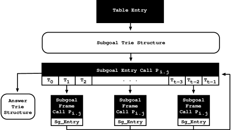
Figure 4: Table space organization for the FS design

In this design, the $AT(P_{i.j})$ structure and part of the subgoal frame information, the subgoal entry data structure in Fig. 4, are now also shared among all threads. The previous $SF$ data structure was split into two: the subgoal entry stores common information for the subgoal call (such as the pointer to the shared $AT(P_{i.j})$ structure) and a $BA$ structure; and the remaining information (the subgoal frame data structure in Fig. 4) is kept private to each thread. Concurrency among threads now includes also the access to the subgoal entry data structure and the allocation of trie nodes on the $AT(P_{i.j})$ structures.

The subgoal entry includes a $BA$ where each thread $T_{k}$ has its own entry which then points to the thread’s private subgoal frame. Each private subgoal frame includes an extra field which is a back pointer to the common subgoal entry. This is important in order to keep unaltered all the tabling data structures that access subgoal frames. To access the private information, there is no extra cost (we still use a direct pointer), and only for the common information on the subgoal entry we pay the extra cost of following an indirect pointer.

Comparing with the NS and SS designs, the FS design has two major advantages. First, memory usage is reduced to a minimum. The only memory overhead, when compared with a single threaded evaluation, is the $BA$ associated with each subgoal entry, and apart from the split on the subgoal frame data structure, all the remaining structures remain unchanged. Second, since threads are sharing the same $AT(P_{i.j})$ structures, answers inserted by a thread for a particular subgoal call are automatically made available to all other threads when they call the same subgoal.

Given an arbitrary number of $NT$ running threads and assuming that all threads have completely evaluated the same number $NC(P_{i})$ of tabled subgoal calls, Eq. 4 shows the memory usage for a predicate $P_{i}$ in the FS design ($MU_{FS}(P_{i})$).

$$MU_{FS}(P_{i})=TE+ST(P_{i})+\sum\limits^{NC(P_{i})}_{j=1}[SE_{FS}+BA+NT*[SF_{FS}+BP]+AT(P_{i.j})]$$ (4)

$$where~{}~{}SE_{FS}+SF_{FS}=SF$$

The memory usage for the FS design is given by the sum of the memory size of the $TE$ and $ST(P_{i})$ data structures plus the summation, for each subgoal call, of the memory used by the subgoal entry data structure ($SE_{FS}$), the $BA$ and the $AT(P_{i.j})$ structures added with the sizes of the private data structures of each thread multiplied by the $NT$ threads. The private data structures of each thread include the subgoal frame ($SF_{FS}$) and the back pointer ($BP$). The memory size of the original $SF$ is now given by the size of the $SE_{FS}$ and $SF_{FS}$ data structures. The memory size of the remaining structures is the same as in Yap’s original table space organization.

Since the FS design is a refinement of the SS design, next we use Thm. 2 to show that the FS design always requires less memory than the SS design for more than one thread.

Theorem 2

If $NT>1$ and $NC(P_{i})\geq 1$ then $MU_{FS}(P_{i})<MU_{SS}(P_{i})$.

Remember from the previous subsection that the SS behavior depends on the amount of memory spent in the $BA$. The FS maintains this dependency, since this structure is co-allocated inside the subgoal entry structure. The difference between both designs occurs in the memory usage spent in the subgoal frames and in the answer tries. For the subgoal frames, the difference is that the size of the private subgoal frames used by the FS design, including the back pointer, is lower that the ones used by the SS design. For the answer trie structures, the FS design simply does not allocate as many of these structures has the SS design. For one thread ($NT=1$), the following corollary can be derived from Thm. 2:

Corollary 3

If $NT=1$ and $NC(P_{i})\geq 1$ then $MU_{FS}(P_{i})>MU_{SS}(P_{i})$.

In summary, for one thread, the FS design is always worse than the SS design and the difference increases proportionally to the number of subgoal calls. For a number of threads higher than one, the FS design always performs better than the SS design and the difference increases as the number of threads and the number of subgoal calls also increases.

3.6 Partial Answer Sharing Design

In the SS design, the subgoal trie structures are shared among threads but the answers for the subgoal calls are stored in private answer trie structures to each thread. As a consequence, no sharing of answers between threads is done. The Partial Answer Sharing (PAS) design [Areias and Rocha (2017)] extends the SS design to allow threads to share answers. Threads still view their answer tries as private but are able to consume answers from completed answer tries computed by other threads. The idea is as follows. Whenever a thread calls a new tabled subgoal, first it searches the table space to lookup if any other thread has already computed the answers for that subgoal. If so, then the thread reuses the available answers, thus avoiding recomputing the subgoal call from scratch. Otherwise, it computes the subgoal itself. Several threads can work on the same subgoal call simultaneously, i.e., we do not protect a subgoal from further evaluations while other threads have picked it up already. The first thread completing a subgoal, shares the results by making them available (public) to the other threads. Figure 5 illustrates the table space organization for the PAS design.

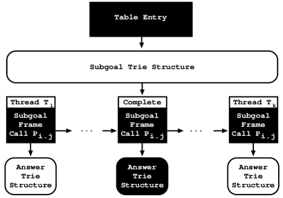
Figure 5: Table space organization for the PAS design

As for the SS design, threads can concurrently access the subgoal trie structures for both read and write operations, but for the answer trie structures, they are only concurrently accessed for reading after completion. All subgoal frames and answer tries are initially private to a thread. Later, when the first subgoal frame is completed, i.e., when we have found the full set of answers for it, it is marked as completed (black answer trie in Fig. 5) and put in the beginning of the list of private subgoal frames (configuration shown in Fig. 5). With the PAS design, we also aim to improve the memory usage of the SS design by removing the $BA$ data structure. This is a direct consequence of the analysis made in Eq. 3 where we have shown that the performance of the SS design is directly affected by the size of the memory used by the $BA$ structures. Thus, instead of pointing to a $BA$ as in the SS design, now the leaf data structure in each subgoal trie path points to a list of private subgoal frames corresponding to the threads evaluating the subgoal call. In order to find the subgoal frame corresponding to a thread, we may have to pay an extra cost for navigating in the list but, once a subgoal frame is completed, we can access it immediately since it is always stored in the beginning of the list.

Given an arbitrary number of $NT$ running threads and assuming that all threads have completely evaluated the same number $NC(P_{i})$ of tabled subgoal calls, Eq. 5 shows the memory usage for a predicate $P_{i}$ in the PAS design ($MU_{PAS}(P_{i})$).

$$MU_{PAS}(P_{i})=TE+ST(P_{i})+\sum\limits^{NC(P_{i})}_{j=1}[NT(P_{i.j})*[SF+AT(P_{i.j})]]$$ (5)

$$where~{}~{}NT(P_{i.j})\leq NT$$

The memory usage for the PAS design is given by the sum of the memory size of the $TE$ and $ST(P_{i})$ data structures plus the summation, for each subgoal call, of the memory used by the private structures of each thread multiplied by $NT(P_{i.j})$ threads, where $NT(P_{i.j})$ is the number of threads evaluating the subgoal call $P_{i.j}$ in a private fashion. Note that $NT(P_{i.j})\leq NT$, since the threads consuming answers from completed subgoal frames do not allocate any extra memory. The memory size of each particular data structure is the same as in Yap’s original table space organization.

In summary, if comparing Eq. 3 with Eq. 5, we can observe that the total memory usage of the PAS design is always less than the total memory usage of the SS design. Additionally, we can optimize even further this design and allow threads to delete their private $SF$ and $AT(P_{i.j})$ structures when completing, if another thread has made public its completed subgoal frame first. With this optimization, we can end in practice with a single $SF$ and $AT(P_{i.j})$ structure for each subgoal call $P_{i.j}$.

If comparing with the FS design, because we only share completed answer tries, we also avoid some problems present in the FS design. First, we avoid the problem of dealing with concurrent updates to the answer tries. Second, we avoid the problem of dealing with concurrent deletes, as in the case of using mode-directed tabling. Since the PAS design keeps the answer tries private to each thread, the deletion of nodes can be done without any complex machinery to deal with concurrent delete operations. Third, we avoid the problem of managing the different set of answers that each thread has found. As we will see in the next subsection, this can be a problem for batched scheduling evaluation.

3.7 Private Answer Chaining Design

During tabled execution, there are several points where we may have to choose between continuing forward execution, backtracking, consuming answers from the tables or completing subgoals. The decision about the evaluation flow is determined by the scheduling strategy. Different strategies may have a significant impact on performance, and may lead to a different ordering of solutions to the query goal. Arguably, the two most successful tabling scheduling strategies are local scheduling and batched scheduling [Freire et al. (1996)].

Local scheduling tries to complete subgoals as soon as possible. When new answers are found, they are added to the table space and the evaluation fails. Local scheduling has the advantage of minimizing the size of clusters of dependent subgoals. However, it delays propagation of answers and requires the complete evaluation of the search space.

Batched scheduling tries to delay the need to move around the search tree by batching the return of answers to consumer subgoals. When new answers are found for a particular tabled subgoal, they are added to the table space and the evaluation continues. Batched scheduling can be a useful strategy in problems which require an eager propagation of answers and/or do not require the complete set of answers to be found.

With the FS design, all tables are shared. Thus, since several threads can be inserting answers in the same answer trie, when an answer already exists, it is not possible to determine if the answer is new or repeated for a particular thread without further support. For local scheduling, this is not a problem since, for repeated and new answers, local scheduling always fails. The problem occurs with batched scheduling that requires that only the repeated answers should fail. Threads have then to detect, during batched evaluation, whether an answer is new and must be propagated or whether an answer is repeated and the evaluation must fail. The Private Answer Chaining (PAC) design [Areias and Rocha (2015a)] extends the FS design to keep track of the answers that were already found and propagated per thread and subgoal call. Figure 6 illustrates PAC’s key idea.

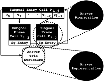
Figure 6: PAC overview

In a nutshell, PAC splits answer propagation from answer representation, and allows the former to be privately stored in the subgoal frame data structure of each thread, and the latter to be kept publicly shared among threads in the answer trie data structure. This is similar to the idea proposed by Costa and Rocha [Costa et al. (2009)] for the global trie data structure, where answers are represented only once on a global trie and then each subgoal call has private pointers to its set of answers. With PAC, we follow the same key idea of representing only once each answer (as given by the FS design), but now since we are in a concurrent environment, we use a private chain of answers per thread to represent the answers for each subgoal call. Later, if a thread completes a subgoal call, its PAC is made public so that from that point on all threads can use that chain in complete (only reading) mode. Figure 7 illustrates the new data structures involved in the implementation of PAC’s design for a situation where different threads are evaluating the same tabled subgoal call $P_{i.j}$.

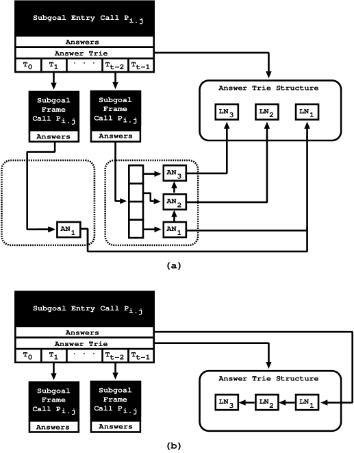
Figure 7: PAC’s data structures for (a) private and (b) public chaining

Figure 7(a) shows then a situation where two threads, $T_{1}$ and $T_{t-2}$, are sharing the same subgoal entry for a call $P_{i.j}$ still under evaluation, i.e., still not yet completed. The current state of the evaluation shows an answer trie with 3 answers found for $P_{i.j}$. For the sake of simplicity, we are omitting the internal answer trie nodes and we are only showing the leaf nodes $LN_{1}$, $LN_{2}$ and $LN_{3}$ of each answer.

With the PAC design, the leaf nodes are not chained in the answer trie data structure, as usual. Now, the chaining process is done privately, and for that, we use the subgoal frame structure of each thread. On the subgoal frame structure we added a new field, called Answers, to store the answers found within the execution of the thread. In order to minimize PAC’s impact, each answer node in the private chaining has only two fields: (i) an entry pointer, which points to the corresponding leaf node in the answer trie data structure; and (ii) a next pointer to chain the nodes in the private chaining. To maintain good performance, when the number of answer nodes exceeds a certain threshold, we use a hash trie mechanism design similar to the one presented in [Areias and Rocha (2015b)], but without concurrency support, since this mechanism is private to each thread.

PAC’s data structures in Fig. 7(a) represent then two different situations. Thread $T_{1}$ has only found one answer and it is using a direct answer chaining to access the leaf node $LN_{1}$. Thread $T_{t-2}$ has already found three answers for $P_{i.j}$ and it is using the hash trie mechanism within its private chaining. In the hash trie mechanism, the answer nodes are still chained between themselves, thus that repeated calls belonging to thread $T_{t-2}$ can consume the answers as in the original mechanism.

Figure 7(b) shows the state of the subgoal call after completion. When a thread $T$ completes a subgoal call, it frees its private consumer structures, but before doing that, it checks whether another thread as already marked the subgoal as completed. If no other thread has done that, then thread $T$ not only follows its private chaining mechanism, as it would for freeing its private nodes, but also follows the pointers to the answer trie leaf nodes in order to create a chain inside the answer trie. Since this procedure is done inside a critical region, no more than one thread can be doing this chaining process. Thus, in Fig. 7(b), we are showing the situation where the subgoal call $P_{i.j}$ is completed and both threads $T_{1}$ and $T_{t-2}$ have already chained the leaf nodes inside the answer trie and removed their private chaining structures.

4 Engine Components

This section discusses the most important engine components required to support concurrent tabled evaluation.

4.1 Fixed-Size Memory Allocator

A critical component in the implementation of an efficient concurrent tabling system is the memory allocator. Conceptually, there are two categories of memory allocators: kernel-level and user-level memory allocators. Kernel-level memory allocators are responsible for managing memory inside the protected sub-systems/resources of the operating system, while user-level memory allocators are responsible for managing the heap area, which is the area inside the addressing space of each process where the dynamic allocation of memory is directly done.

Evidence of the importance of a User-level Memory Allocator (UMA) comes from the wide array of UMA replacement packages that are currently available. Some examples are the PtMalloc [(27)], Hoard [Berger et al. (2000)], TcMalloc [(25)] and JeMalloc [Evans (2006)] memory allocators. Many UMA subsystems were written in a time when multiprocessor systems were rare. They used memory efficiently but were highly serial, constituting an obstacle to the throughput of concurrent applications, which require some form of synchronization to protect the heap. Additionally, when a concurrent application is ran in a multiprocessor system, other problems can occur, such heap blowup, false sharing or memory contention [Masmano et al. (2006), Gidenstam et al. (2010)].

Since tabling also demands the multiple allocation and deallocation of different sized chunks of memory, memory management plays an important role in the efficiency of a concurrent tabling system. To satisfy this demand, we have designed a fixed-size UMA especially aimed for an environment with the characteristics of concurrent tabling [Areias and Rocha (2012a)]. In a nutshell, fixed-size UMA separates local and shared memory allocation, and uses local and global heaps with pages that are formatted in blocks with the sizes of the existing data structures. The page formatting in blocks contributes to avoid inducing false-sharing, because different threads in different processors do not share the same cache lines, and to avoid the heap blowup problem, because pages migrate between local and global heaps.

At the implementation level, our proposal has local and global heaps with pages formatted for each object type. In addition, global and local heaps can hold free (unformatted) pages for use when a local heap runs empty. Since modern computer architectures use pages to handle memory, we adopted an allocation scheme based also on pages, where each memory page only contains data structures of the same type. In order to split memory among different threads, in our proposal, a page can be considered a local page, if owned by a particular thread, or a global page, otherwise. Figure 8 gives an overview of this organization.

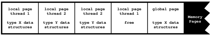
Figure 8: Using pages as the basis for the fixed-size memory allocator

A thread can own any number of pages of the same type, of different types and/or free pages. Any type of page (including free pages) can be local to a thread or global, and each particular page only contains data structures of the same type. When a page $P$ is made local to a thread $T$, it means that $T$ gains exclusive permission to allocate and deallocate data structures on $P$. On the other hand, global pages have no owners and, thus, they are free from allocate/deallocate operations. To allocate/deallocate data structures on global pages, first the corresponding pages should be moved to a particular thread. All running threads can access (for read or write operations) the data structures allocated on a page, independently of being a local or global page.

Allocating and freeing data structures are constant-time operations, because they require only moving a structure to or from a list of free structures. Whenever a thread $T$ requests to allocate memory for a data structure of type $S$, it can instantly satisfy the request by returning the first unused slot on the first available local page with type $S$. Deallocation of a data structure of type $S$ does not free up the memory, but only opens an unused slot on the chain of available local pages for type $S$. Further requests to allocate memory of type $S$ will later return the now unused memory slot. When all data structures in a page are unused, the page is moved to the chain of free local pages. A free local page can be reassigned later to a different data type. When a thread $T$ runs out of available free local pages, it must synchronize with the other threads in order to access the global pages or the operating system’s memory allocator, if no free global page exists. This process eliminates the need to search for suitable memory space and greatly alleviates memory fragmentation. The only wasted space is the unused portion at the end of a page when it cannot fit exactly with the size of the corresponding data structures.

When a thread finishes execution, it deallocates all its private data structures and then moves its local pages to the corresponding global page entries. Shared structures are only deallocated when the last running thread (usually the main thread) abolishes the tables. Thus, if a thread $T$ allocates a data structure $D$, then it will be also responsible for deallocating $D$, if $D$ is private to $T$, or $D$ will remain live in the tables, if $D$ is shared, even when $T$ finish execution. In the latter case, $D$ can be only deallocated by the last running thread $L$. In such case, $D$ is made to be local to $L$ and the deallocation process follows as usual.

4.2 Lock-Free Data Structures

Another critical component in the implementation of an efficient concurrent tabling system is the design of the data structures and algorithms that manipulate shared tabled data. As discussed before, Yap’s table space follows a two-level trie data structure, where one level stores the tabled subgoal calls and the other stores the computed answers. Depending on the number of subgoal calls or answers, the paths inside a trie, corresponding to the subgoal calls or answers, might have several trie nodes per internal level of the trie structure. Whenever an internal trie level becomes saturated, a hash mechanism is used to provide direct node access and therefore optimize the search for the data within the trie level. Figure 9 shows a hashing mechanism for an internal trie level within the subgoal and answer data structures.

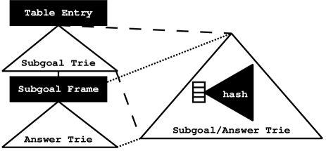
Figure 9: The hashing mechanism within a trie level

Several approaches for hashing mechanisms exist. The most important aspect of a hashing mechanism is its behavior in terms of hash collisions, i.e., when two keys collide and occupy the same hash table location. Multiple solutions exist that address the collision problem. Among these are the open addressing and closed addressing approaches [Tenenbaum et al. (1990), Knuth (1998)]. In open addressing, the hash table stores the objects directly within the hash table internal array, while in closed addressing, every object is stored directly at an index in the hash table’s internal array. In closed addressing, collisions are solved by using other arrays or linked lists. Yap’s tabling engine uses separate chaining [Knuth (1998)] to solve hash collisions. In the separate chaining mechanism, the hash table is implemented as an array of linked lists. The basic idea of separate chaining techniques is to apply linked lists for collision management, thus in case of a conflict a new object is appended to the linked list.

Our initial approach to deal with concurrency within the trie structures was to use lock-based strategies [Areias and Rocha (2012b)]. However, lock-based data structures have their performance restrained by multiple problems, such as, convoying, low fault tolerance and delays occurred inside a critical region. We thus shifted our attention in to taking advantage of the low-level Compare-And-Swap (CAS) operation, that nowadays can be widely found on many common architectures. The CAS operation is an atomic instruction that compares the contents of a memory location to a given value and, if they are the same, updates the contents of that memory location to a given new value. The CAS operation is at the heart of many lock-free (also known as non-blocking) data structures [Herlihy and Wing (1987)]. Non-blocking data structures offer several advantages over their blocking counterparts, such as being immune to deadlocks, lock convoying and priority inversion, and being preemption tolerant, which ensures similar performance regardless of the thread scheduling policy. Using lock-free techniques, we have created two proposals for concurrent hashing data structures especially aimed to be as effective as possible in a concurrent tabling engine and without introducing significant overheads in the sequential execution. Figure 10 shows the architecture of the two proposals.

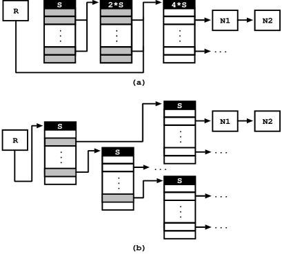
Figure 10: Architecture of the two lock-free hash proposals

Both proposals include a root node $R$ and have a hashing mechanism composed by a bucket array and a hash function that maps the nodes into the entries in the bucket array. The first proposal, shown in Fig. 10(a), implements a dynamic resizing of the hash tables by doubling the size of the bucket array whenever it becomes saturated [Areias and Rocha (2014)]. It starts with an initial bucket array with $S$ entries and, whenever the hash bucket array becomes saturated, i.e., when the number of nodes in a bucket entry exceeds a pre-defined threshold value and the total number of nodes exceeds $S$, then the bucket array is expanded to a new one with $2*S$ entries. This expansion mechanism is executed by a single thread, meaning that no more than one expansion can be done at a time. If the thread executing the expansion suspends for some reason (for example, be suspended by the operating system scheduler), then all the remaining threads can still be searching and inserting nodes in the trie level that is being expanded in a lock-free fashion, but no other thread will be able to expand the same trie level. When the process of bucket expansion is completed for all $S$ bucket entries, node $R$ is updated to refer to the new bucket array with $2*S$ entries. Since the size of the hashes doubles on each expansion, this proposal is highly inappropriate to be integrated with the fixed-size UMA.

The second proposal, shown in Fig. 10(b), was designed to be compatible with the fixed-size UMA. It is based on hash tries data structures and is aimed to be a simpler and more efficient lock-free proposal that disperses the synchronization regions as much as possible in order to minimize problems such as false sharing or cache memory ping pong effects [Areias and Rocha (2015b)]. Hash tries (or hash array mapped tries) are another trie-based data structure with nearly ideal characteristics for the implementation of hash tables [Bagwell (2001)]. As shown in Fig. 9, in this proposal, we still have the original subgoal/answer trie data structures which include a hashing mechanism whenever an internal trie level becomes saturated, but now the hashing mechanism is implemented using hash tries data structures.

An essential property of the trie data structure is that common prefixes are stored only once [Fredkin (1962)], which in the context of hash tables allows us to efficiently solve the problems of setting the size of the initial hash table and of dynamically resizing it in order to deal with hash collisions. In a nutshell, a hash trie is composed by internal hash arrays and leaf nodes (nodes $N1$ and $N2$ in Fig. 10(b)) and the internal hash arrays implement a hierarchy of hash levels of fixed size $S=2^{w}$. To map a node into this hierarchy, first we compute the hash value $h$ and then we use chunks of $w$ bits from $h$ to index the entry in the appropriate hash level. Hash collisions are solved by simply walking down the tree as we consume successive chunks of $w$ bits from the hash value $h$. Whenever a hash bucket array becomes saturated, i.e., when the number of nodes in a bucket entry exceeds a pre-defined threshold value, then the bucket array is expanded to a new one with $S$ entries. As for the previous proposal, this expansion mechanism is executed by a single thread. If the thread executing the expansion suspends for some reason, then all the remaining threads can still be searching and inserting nodes in the bucket entry in a lock-free fashion. Compared with the previous proposal, this proposal has a fined grain synchronization region, because it blocks only one bucket entry per expansion.

5 Performance Analysis

Our work on combining tabling with parallelism started some years ago when the first approach for implicit parallel tabling was presented [Rocha et al. (1999)]. Such approach lead to the design and implementation of an or-parallel tabling system, named OPTYap [Rocha et al. (2001)]. In OPTYap, each worker behaves like a sequential tabling engine that fully implements all the tabling operations. During the evaluation, the or-parallel component of the system is triggered to allow synchronized access to the table space and to the common parts of the search tree, or to schedule workers running out of alternatives to exploit.

OPTYap has shown promising results in several tabled benchmarks [Rocha et al. (2001)]. The worst results were obtained in the transitive closure of the right recursive definition of the path problem using a grid configuration, where no speedups were obtained with multiple workers. The bad results achieved in this benchmark were explained by the higher rate of contention in Yap’s internal data structures, namely in the subgoal frames. A closer analysis showed that the number of suspension/resumptions operations is approximately constant with the increase in the number of workers, thus suggesting that there are answers that can only be found when other answers are also found, and that the process of finding such answers cannot be anticipated. In consequence, suspended branches have always to be resumed to consume the answers that could not be found sooner.

More recently, we shifted our research towards explicit parallelism specially aimed for multithreaded environments. Initial results were promising as we were able to significantly reduce the contention for concurrent table accesses [Areias and Rocha (2012b), Areias and Rocha (2012a)]. Later, we presented first speedup results for the right recursive definition of the path problem, using a naive multithreaded scheduler that considers a set of different starting points (queries) in the graph to be run by a set of different threads. In this work, Yap obtained a maximum speedup of $10.24$ for 16 threads [Areias and Rocha (2015b)]. Although, these results were better than the ones presented earlier for implicit parallelism, they were mostly due to the different scheduler strategy adopted to evaluate the benchmark. On the other hand, such work also showed that with 32 threads, no improvements were obtained compared with 16 threads. A closer analysis showed again that such behavior was related with the large number of subgoal call dependencies in the program. We thus believe that the ordering to which the answers are found in some problems, like in the evaluation of the transitive closure of strongly connected graphs, is a major problem that restricts concurrency/parallelism in tabled programs.

In what follows, we start with worst case scenarios to study how independent flows of execution running simultaneously interfere at the low-level engine. Next, we focus on two well-known dynamic programming problems, the Knapsack and LCS problems, and we discuss how we were able to scale their execution by using Yap’s multithreaded tabling engine. The environment of our experiments was a machine with 32-Core AMD Opteron (TM) Processor 6274 (2 sockets with 16 cores each) with 32GB of main memory, running the Linux kernel 3.16.7-200.fc20.x86 64 with Yap Prolog 6.3.

5.1 Experiments on Worst Case Scenarios

We begin with experimental results for concurrent tabled evaluation using local and batched scheduling with the NS, SS and PAC designs for worst case scenarios that stress the trie data structures. For the sake of simplicity, we will present only the best results, which were always achieved when using the fixed-size UMA and the second lock-free proposal. We do not show results for the CS and PAS designs because they are not meaningful in this context, as we will see next. The results for the FS design are identical to PAC’s results, except for batched scheduling which FS does not support.

For benchmarking, we used the set of tabling benchmarks from [Areias and Rocha (2012a)] which includes 19 different programs in total. We choose these benchmarks because they have characteristics that cover a wide number of scenarios in terms of trie usage. They create different trie configurations with lower and higher number of nodes and depths, and also have different demands in terms of trie traversing.

To create worst case scenarios that stress the table data structures, we ran all threads starting with the same query goal. By doing this, it is expected that threads will access the table space, to check/insert for subgoals and answers at similar times, thus causing a huge stress on the same critical regions. In particular, for this set of benchmarks, this will be especially the case for the answer tries, since the number of answers clearly exceeds the number of subgoals. Please note that, despite all threads are executing the same program they have independent flows of execution, i.e., we are not trying to parallelize the execution, but study how independent flows of execution (in this case, identical flows of execution) interfere at the low-level engine. By focusing first on the worst case scenarios, we can infer the highest overhead ratios when compared with one thread (or the lowest bounds of performance) that each design might have when used with multiple threads in other real world applications. For each table design, there are two main sources of overheads: (i) the synchronization required to interact with the memory allocator, which is proportional to the memory consumption bounds discussed in Section 3; and (ii) the synchronization required to interact with the table space, which is proportional to the number of data structures that can be accessed concurrently in each design. The overheads originated from these two sources are not easy to isolate in order to evaluate the weight of each in the execution time. The design of the memory allocator clearly plays an important role in the former source of overhead and the use of lock-free data structures is important to soften the weight of the latter.

Table 2 shows the overhead ratios, when compared with the NS design with 1 thread (running with local scheduling and without the fixed-size UMA) for the NS, SS and PAC designs running 1, 8, 16, 24 and 32 threads with local and batched scheduling on the set of benchmarks. In order to give a fair weight to each benchmark, the overhead ratio is calculated as follows. We begin by running ten times each benchmark $B$ for each design $D$ with $T$ threads. Then, we calculate the average of those ten runs and use that value ($D_{BT}$) to put it in perspective against the base time, which is the average of the ten runs of the NS design with one thread ($NS_{B1}$). For that, we use the following formula for the overhead $O_{DBT}=D_{BT}/NS_{B1}$. After calculating all the overheads $O_{DBT}$ for a certain design $D$ and number of threads $T$ corresponding to the several benchmarks $B$, we calculate the respective minimum, average, maximum and standard deviation overhead ratios. The higher the overhead, the worse the design behaves. An overhead of 1.00 means that the design behaves similarly to the base case and is thus immune to the fact of having other execution flows running simultaneously.

Table 2: Overhead ratios, when compared with the NS design with 1 thread (running with local scheduling and without the fixed-size UMA), for the NS, SS and PAC designs running 1, 8, 16, 24 and 32 threads with local and batched scheduling (best ratios by row and by design for the Minimum, Average and Maximum are in bold)

Threads		NS		SS		PAC
		Local	Batched	Local	Batched	Local	Batched
1	Min	0.53	0.55	0.54	0.55	1.01	0.95
	Avg	0.78	0.82	0.84	0.90	1.30	1.46
	Max	1.06	1.05	1.04	1.04	1.76	2.33
	StD	0.15	0.14	0.17	0.16	0.22	0.44
8	Min	0.66	0.63	0.66	0.63	1.16	0.99
	Avg	0.85	0.88	0.92	0.93	1.88	1.95
	Max	1.12	1.14	1.20	1.15	2.82	3.49
	StD	0.13	0.14	0.15	0.14	0.60	0.79
16	Min	0.85	0.75	0.82	0.77	1.17	1.06
	Avg	0.98	1.00	1.04	1.05	1.97	2.08
	Max	1.16	1.31	1.31	1.28	3.14	3.69
	StD	0.09	0.17	0.12	0.13	0.65	0.83
24	Min	0.91	0.93	1.02	0.98	1.16	1.09
	Avg	1.15	1.16	1.22	1.19	2.06	2.19
	Max	1.72	1.60	1.81	1.61	3.49	4.08
	StD	0.20	0.21	0.18	0.16	0.70	0.91
32	Min	1.05	1.04	1.07	1.12	1.33	1.26
	Avg	1.51	1.49	1.54	1.51	2.24	2.41
	Max	2.52	2.63	2.52	2.62	3.71	4.51
	StD	0.45	0.45	0.42	0.43	0.74	1.02

By observing Table 2, we can notice that for one thread, on average, local scheduling is sightly better than batched on the three designs. As we increase the number of threads, one can observe that, for the NS and SS designs, both scheduling strategies show very close minimum, average and maximum overhead ratios. For the PAC design, the best minimum overhead ratio is always for batched scheduling but, for the average and maximum overhead ratio, local scheduling is always better than batched scheduling. For the average and maximum overhead ratios, the difference between local and batched scheduling in the PAC design is slightly higher than in the NS and SS designs, which can be read as an indication of the overhead that PAC introduces into the FS design. Recall that whenever an answer is found during the evaluation, PAC requires that threads traverse their private consumer data structures to check if the answer was already found (and propagated).

Finally, we would like to draw the reader’s attention to the worst results obtained (the ones represented by the maximum rows). For 32 threads, the NS, SS and PAC designs have overhead results of 2.52/2.63, 2.52/2.62 and 3.71/4.51, respectively for local/batched scheduling. These are outstanding results if we compare them with the results obtained in our first approach [Areias and Rocha (2012b)], without the fixed-size UMA and without lock-free data structures, where for local scheduling with 24 threads, the NS, SS and FS designs had average overhead results of 18.64, 17.72 and 5.42, and worst overhead results of 47.89, 47.60 and 11.49, respectively. Results for the XSB Prolog system, also presented in [Areias and Rocha (2012b)], for the same set of benchmarks showed average overhead results of 6.1 and worst overhead results of 10.31. We thus argue that the combination of a fixed-size UMA with lock-free data structures is the best proposal to support concurrency in general purpose multithreaded tabling applications.

5.2 Experiments on Dynamic Programming Problems

As mentioned in subsection 3.1, with a fully explicit approach, it is left to the user to break the problem into tasks for concurrent execution, assign them to the available workers and control the execution and the synchronization points, i.e., it is not the tabled execution system that is responsible for doing that, the execution system only provides the mechanisms/interface for allowing simultaneous flows of execution. Thus, the user-level scheduler implemented by the user, to support the division of the problem in concurrent tasks and control the execution and synchronization points, plays a key role in the process of trying to obtain speedups through parallel execution. This means that we cannot evaluate the infrastructure of a concurrent tabling engine just by running some benchmarks if we do not put a big effort in a good scheduler design, which is independent from such infrastructure.

In this subsection, we show how dynamic programming problems fit well with concurrent tabled evaluation [Areias and Rocha (2017)]. To do so, we used two well-known dynamic programming problems, the Knapsack and the Longest Common Subsequence (LCS) problems. The Knapsack problem [Martello and Toth (1990)] is a well-known problem in combinatorial optimization that can be found in many domains such as logistics, manufacturing, finance or telecommunications. Given a set of items, each with a weight and a profit, the goal is to determine the number of items of each kind to include in a collection so that the total weight is equal or less than a given capacity and the total profit is as much as possible. The problem of computing the length of the LCS is representative of a class of dynamic programming algorithms for string comparison that are based on getting a similarity degree. A good example is the sequence alignment, which is a fundamental technique for biologists to investigate the similarity between species.

For the Knapsack problem, we fixed the number of items and capacity, respectively, 1,600 and 3,200. For the LCS problem, we used sequences with a fixed size of 3,200 symbols. Then, for each problem, we created three different datasets, D₁₀, D₃₀ and D₅₀, meaning that the values for the weights/profits for the Knapsack problem and the symbols for LCS problem where randomly generated in an interval between 1 and 10%, 30% and 50% of the total number of items/symbols, respectively.

For both problems, we implemented either multithreaded tabled top-down and multithreaded tabled bottom-up user-level scheduler approaches. For the top-down approaches, we followed Stivala et al.’s work [Stivala et al. (2010)] where a set of threads solve the entire program independently but with a randomized choice of the sub-problems. Figure 11 illustrates how this was applied in the case of the Knapsack problem considering $N$ items and $C$ capacity. A set of threads begin the execution with the same top query tabled call, $ks(N,C)$ in Fig. 11, but then, on each level of the evaluation tree, each thread randomly decides which branch will be evaluated first, the exclude item branch (Exc) or the include item branch (Inc). This random decision is aimed to disperse the threads through the evaluation tree.

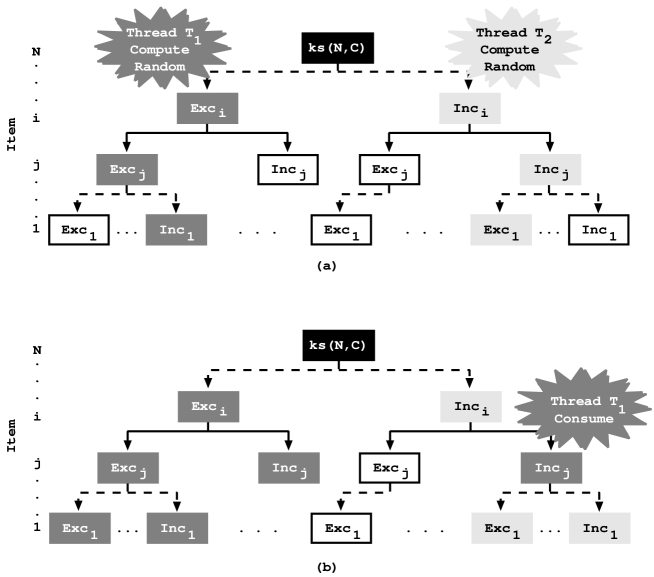
Figure 11: Knapsack multithreaded tabled top-down approach

Figure 11(a) shows a situation where, starting from a certain item i and capacity, thread $T_{1}$ is evaluating the left branch of the tree ($Exc_{i}$), while thread $T_{2}$ is evaluating the right branch ($Inc_{i}$). Notice that although the threads are evaluating the branches of the tree in a random order, they still have to evaluate all branches so that they can find the optimal solution for the Knapsack problem. So, the random decision is only about the evaluation order of the branches and not about skipping branches. Figure 11(b) shows then a situation where thread $T_{1}$ has completely evaluated the $Exc_{i}$ branch of the tree and has moved to the $Inc_{i}$ branch where it is now evaluating a $Inc_{j}$ branch already evaluated by thread $T_{2}$. Since the result for that branch is already stored in the corresponding table, thread $T_{1}$ simply consumes the result, thus avoiding its computation.

For each sub-problem, two alternative execution choices are available: (i) exclude first and include next, or (ii) include first and exclude next. The randomized choice of sub-problems results in the threads diverging to compute different sub-problems simultaneously while reusing the sub-problem’s results computed in the meantime by the other threads. Since the number of sub-problem is usually high in this kind of problems, it is expected that the available set of sub-problems will be evenly divided by the number of available threads resulting in less computation time required to reach the final result.

We have implemented two alternative versions. The first version (YAP${}_{TD_{1}}$) simply follows Stivala et al.’s original random approach. The second version (YAP${}_{TD_{2}}$) extends the first one with an extra step where the computation is first moved forward (i.e., to a deeper item/symbol in the evaluation tree) using a random displacement of the number of items/symbols (we used a $maxRandom$ value corresponding to $10\%$ of the total number of items/symbols in the problem) and only then the computation is performed for the next item/symbol, as usual.

For the bottom-up user-level scheduler approaches (YAP_BU), the Knapsack version is based on [Kumar et al. (1994)] and the LCS version is based on [Kumar (2002)]. Figure 12 illustrates the case of the Knapsack problem for $N$ items and $C$ capacity. The evaluation is done bottom-up with increasing capacities $c\in\{1,...,C\}$ until computing the maximum profit for the given capacity $C$, which corresponds to the query goal $ks(N,C)$. The bottom-up characteristic comes from the fact that, given a Knapsack with capacity $c$ and using $i$ items, $i<N$, the decision to include the next item $j$, $j=i+1$, leads to two situations: (i) if $j$ is not included, the Knapsack profit is unchanged; (ii) if $j$ is included, the profit is the result of the maximum profit of the Knapsack with the same $i$ items but with capacity $c-w_{j}$ (the capacity needed to include the weight $w_{j}$ of item $j$) increased by $p_{j}$ (the profit of the item $j$ being included). The algorithm then decides whether to include an item based on which choice leads to maximum profit. Thus, computing a row $i$ depends only on the sub-problems at row $i-1$. A possible parallelization is, for each row, to divide the computation of the $C$ columns between the available threads and then wait for all threads to complete in order to synchronize before computing the next row. Figure 12(a) shows an example with two threads, $T_{1}$ and $T_{2}$, where the computation of the $C$ columns within the evaluation matrix is divided in smaller chunks and each chunk is evaluated by the same thread.

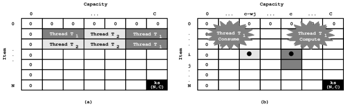
Figure 12: Knapsack multithreaded tabled bottom-up approach

Figure 12(b) shows then a situation where the cell corresponding to call $ks(j,c)$ is being evaluated by thread $T_{1}$. As explained above, this involves computing the values for $ks(i,c-w_{j})$ and $ks(i,c)$ (cells denoted with a black circle in Fig.12(b)). Since we want to take advantage of the built-in tabling mechanism, we can avoid the synchronization between rows mentioned above. Hence, when a sub-problem in the previous row was not computed yet (i.e., marked as completed in one of the subgoal frames for the given call), instead of waiting for the corresponding result to be computed by another thread, the current thread starts also its computation and for that it can recursively call many other sub-problems not computed yet. Despite this can lead to redundant sub-computations, it avoids synchronization. In fact, as we will see, this approach showed to be very effective. The situation in Fig. 12(b) shows the case where thread $T_{1}$ consumes the value for call $ks(i,c-w_{j})$ from the tables (already computed by $T_{2}$) but computes the value for $ks(i,c)$.

To evaluate the performance of the multithreaded tabled top-down and bottom-up approaches, we used local scheduling with the PAS design, together with the fixed-size UMA and the support for lock-free data structures within the subgoal trie data structure. For the bottom-up approaches, standard tabling is enough but for the top-down approaches, mode-directed tabling is mandatory since we want to maximize the profit, in the case of the Knapsack problem, and the length of the longest common subsequence, in the case of the LCS problem. To put our results in perspective, we also experimented with XSB Prolog version 3.4.0 using the shared tables model [Marques and Swift (2008)] for the bottom-up approaches (since XSB does not support mode-directed tabling, it could not be used for the top-down approaches).

Table 3: Execution time, in milliseconds, for one thread (sequential and multithreaded version) and corresponding speedup (against one thread running the multithreaded version) for the execution with 8, 16, 24 and 32 threads, for the top-down and bottom-up approaches of the Knapsack problem using the Yap and XSB Prolog systems

System/Dataset		Seq.	# Threads (p)					Best
		Time	Time (T1)	Speedup (T1/Tp)				Time
		(Tseq)	1	8	16	24	32	(Tbest)
Top-Down Approaches
YAP${}_{TD_{1}}$	D10	14,330	19,316	1.96	2.12	2.04	1.95	9,115
	D30	14,725	19,332	3.57	4.17	4.06	3.93	4,639
	D50	14,729	18,857	4.74	6.28	6.44	6.41	2,930
YAP${}_{TD_{2}}$	D10	19,667	24,444	6.78	12.35	15.44	18.19	1,344
	D30	19,847	25,609	7.15	13.83	17.37	20.47	1,251
	D50	19,985	25,429	7.27	13.70	17.35	20.62	1,233
Bottom-Up Approaches
YAPBU	D10	12,614	17,940	7.17	13.97	18.31	22.15	810
	D30	12,364	17,856	7.23	13.78	18.26	21.94	814
	D50	12,653	17,499	7.25	14.01	18.34	21.76	804
XSBBU	D10	32,297	38,965	0.87	0.66	0.62	0.55	32,297
	D30	32,063	38,007	0.86	0.61	0.56	0.53	32,063
	D50	31,893	38,534	0.84	0.58	0.57	0.57	31,893

Table 4: Execution time, in milliseconds, for one thread (sequential and multithreaded version) and corresponding speedup (against one thread running the multithreaded version) for the execution with 8, 16, 24 and 32 threads, for the top-down and bottom-up approaches of the LCS problem using the Yap and XSB Prolog systems

System/Dataset		Seq.	# Threads (p)					Best
		Time	Time (T1)	Speedup (T1/Tp)				Time
		(Tseq)	1	8	16	24	32	(Tbest)
Top-Down Approaches
YAP${}_{TD_{1}}$	D10	26,030	33,969	1.58	1.53	1.50	1.42	21,509
	D30	26,523	34,213	1.60	1.54	1.50	1.42	21,424
	D50	26,545	34,234	1.60	1.54	1.51	1.40	21,408
YAP${}_{TD_{2}}$	D10	34,565	44,371	7.23	13.23	16.45	19.74	2,248
	D30	34,284	44,191	7.12	13.09	16.52	19.77	2,235
	D50	33,989	44,158	7.06	13.30	16.49	19.58	2,255
Bottom-Up Approaches
YAPBU	D10	20,799	28,909	6.47	12.21	16.48	20.32	1,423
	D30	21,174	28,904	6.94	12.61	16.63	20.40	1,417
	D50	21,166	28,857	6.44	12.31	16.44	20.52	1,406
XSBBU	D10	60,983	74,108	n.a.	n.a.	n.a.	n.a.	60,983
	D30	59,496	74,410	n.a.	n.a.	n.a.	n.a.	59,496
	D50	59,700	74,628	n.a.	n.a.	n.a.	n.a.	59,700

Table 3 and Table 4 show the average of 10 runs results obtained, respectively, for the Knapsack and LCS problems for both top-down and bottom-up approaches using the Yap and XSB Prolog systems. The columns of both tables show the following information. The first column describes the system and the dataset used. The second column (T_seq) shows the sequential execution time in milliseconds. For T_seq, the Prolog systems where compiled without multithreaded support and ran without multithreaded code. The next five columns show the execution time for one thread (T₁) and the corresponding speedup for the execution with 8, 16, 24 and 32 threads (columns T₁/T_p). For each system/dataset configuration, the results in bold highlight the column where the best execution time was obtained and the last column (T_best) presents such result in milliseconds.

Analyzing the general picture of both tables, one can observe that the sequential time (T_seq) is always lower than the multithreaded time (T₁). This is expected since the multithreaded version is compiled and equipped with all the complex machinery required to support concurrency in Yap, which includes not only all the new tabled stuff but also all the base support for multithreaded in Yap.

When scaling the problem with multiple threads, the YAP${}_{TD_{2}}$ top-down and YAP_BU bottom-up approaches have the best results with excellent speedups for 8, 16, 24 and 32 threads. In particular, for 32 threads, they obtain speedups around 21 and 20, respectively, for the Knapsack and LCS problems (T₁/T_best). If comparing against the sequential version for 32 threads (not shown in the tables), the speedups are around 15 and 16, respectively, for the Knapsack and LCS problems (T_seq/T_best). The results for the top-down YAP${}_{TD_{1}}$ approach are not so interesting, regardless of the fact that it can slightly scale for the Knapsack problem up to 16 threads.

Despite the similar average speedups for YAP${}_{TD_{2}}$ and YAP_BU, their execution times are quite different. Consider, for example, the $D_{50}$ dataset of the Knapsack problem with 32 threads. While the speedup $20.62$ of YAP${}_{TD_{2}}$ corresponds to an execution time of $1,233$ milliseconds, the speedup $21.76$ of YAP_BU only corresponds to $804$ milliseconds. Similarly, for the LCS problem, if considering the $D_{50}$ dataset with 32 threads, while the speedup $19.58$ of YAP${}_{TD_{2}}$ corresponds to $2,255$ milliseconds, the speedup $20.52$ of the YAP_BU only corresponds to $1,406$ milliseconds.

The results also suggest that the execution times are not affected by the values for the weights/profits generated. In general, the speedups obtained for the different datasets ($D_{10}$, $D_{30}$ and $D_{50}$) are always very close for the same number of threads. Note that for the bottom-up approaches this was expected since the complete matrix of results has to be computed. For the top-down approaches, it can be affected by the values for the weights/profits due to the depth in the evaluation tree where solutions can be found. However, since we are using randomized values in the datasets, we are aiming for the average case.

Regarding the comparison with XSB’s shared tables model, Yap’s results clearly outperform those of XSB. For the execution time with one thread, XSB shows higher times than all Yap’s approaches. For the concurrent execution of the Knapsack problem, XSB shows no speedups and for the concurrent execution of the LCS problem we have no results available ($n.a.$) since we got segmentation fault execution errors. From our point of view, XSB’s results are a consequence of the usurpation operation [Marques and Swift (2008)] that restricts the potential of concurrency to non-mutually dependent sub-computations. As the concurrent versions of the Knapsack and LCS problems create mutual dependent sub-computations, which can be executed in different threads, the XSB is actually unable to execute them concurrently. In other works, even if we launch an arbitrary large number of threads on those programs, the system would tend to use only one thread at the end to evaluate most of the computations.

6 Future Perspectives and Challenging Research Directions

Currently, Yap provides the ground technology for both implicit and explicit concurrent tabled evaluation, but separately. From the user’s point of view, tabling can be enabled through the use of single directives of the form ‘:- table p/n’, meaning that common sub-computations for p/n will be synchronized and shared between workers at the engine level, i.e., at the level of the tables where the results for such sub-computations are stored. Implicit concurrent tabled evaluation can be triggered if using the OPTYap design [Rocha et al. (2005)], which exploits implicit or-parallelism using shared memory processes. Explicit concurrent tabled evaluation can be triggered if using the thread-based implementation [Areias and Rocha (2012b)], but the user still needs to explicitly implement the thread management and scheduler policy for task distribution, which is orthogonal to the focus of this work. Table 5 highlights the key differences between the two concurrent tabling strategies in Yap’s current implementation.

Table 5: Concurrent tabling supported features

Strategy	Execution	Memory	Synchronization	Mode-Directed
	Model	Allocator	Mechanisms	Tabling
Implicit	Processes/Threads	Fixed-Size	Lock-Based	–
Explicit	Threads	Fixed-Size	Lock-Free	NS/SS/PAS Designs

The present work could thus be viewed as the basis to further directions and further research in this area. So far, we have achieved our initial goal. Even so, the system still has some restrictions that may reduce its use elsewhere and its contribution to general Prolog applications. We next discuss future perspectives and challenging research directions:

Extend CS design to support lock-free data structures.

Due to the good performance results obtained with the lock-free proposals, an obvious research direction for further work is to extend the original CS design to use lock-free data structures instead of the lock-based data structures.

Extend CS/FS/PAC designs to support mode-directed tabling.

In the previous section, we observed the advantages of combining mode-directed tabling with the PAS design. However, in the PAS design, the answers to common tabled subgoal calls are only shared when the corresponding tables are completed. Since the CS/FS/PAC designs do not require the completion of tables to share answers, threads would be able to share and propagate answers sooner. The problem of combining mode-directed tabling with the CS/FS/PAC designs is on how to efficiently support concurrent delete operations on the trie structures and on how to efficiently handle the interface between consumer calls and the navigation in the trie of answers for the several running workers.

Support concurrent delete operations on the trie structures.

As mention above, this is a key feature to allow for an efficient implementation of concurrent mode-directed tabling with the CS/FS/PAC designs. Moreover, this extension could also be applied to concurrent incremental tabling [Saha (2006)], where specific subgoal calls and answers can be dynamically deleted during tabled evaluation.

Concurrent linear tabling.

Since the evaluation of programs with a linear tabling engine is less complex than the evaluation with a suspension-based engine, it would be interesting to study how different linear tabled strategies [Areias and Rocha (2011), Areias and Rocha (2013)] could run concurrently and take advantage of the different table space designs presented in this work.

Implicit and explicit concurrent evaluation in a single framework.

This is our most challenging goal towards an efficient concurrent framework which integrates both implicit and explicit concurrent tabled evaluation in a single tabling engine. This is a very complex task since we need to combine the explicit control required to launch, assign and schedule tasks to workers, with the built-in mechanisms for handling tabling and/or implicit concurrency, which cannot be controlled by the user. In such a framework, a program begins as a single worker that executes sequentially until reaching an implicit or explicit concurrent construct. When reaching an explicit concurrent construct, the execution model launches a set of additional workers to exploit concurrently a set of independent sub-computations (which may include tabled and non-tabled predicates). From the workers point of view, each concurrent sub-computation computes its tables but, at the implementation level, the tables can be shared following the table space designs presented before for implicit concurrent tabled evaluation. Otherwise, if reaching an explicit concurrent construct, the execution model launches a set of additional workers to exploit in parallel a given sub-computation. Parallel execution is then handled implicitly by the execution model taking into account possible directive restrictions. For example, we may have directives to define the number of workers, the scheduling strategy to be used, load balancing policies, etc. By taking advantage of these explicit parallel constructs, a user can write parallel logic programs from scratch or parallelise existing sequential programs by incrementally pinpointing the sub-computations that can benefit from parallelism, using the available directives to test and fine tune the program in order to achieve the best performance. Such a framework could renew the glamour of Prolog systems, especially in the concurrent/parallel programming community. Combining the inherent implicit parallelism of Prolog with explicit high-level parallel constructs will clearly enhance the expressiveness and declarative style of tabling and simplify concurrent programming.

Appendix A Proofs

Theorem 1

If $NT\geq 1$ and $NC(P_{i})\geq 1$ then $MU_{SS}(P_{i})\leq MU_{NS}(P_{i})$ if and only if the formula $[NC(P_{i})-1]*BA\leq[NT-1]*ST(P_{i})$ holds.

Proof A.2.

Assuming that all tabled subgoal calls are completely evaluated, for the NS design we have:

$$MU_{NS}(P_{i}) =TE+BA+NT*ST(P_{i})+NT*\sum\limits^{NC(P_{i})}_{j=1}[SF+AT(P_{i.j})]$$

And, for the SS design we have:

$$MU_{SS}(P_{i}) =TE+ST(P_{i})+\sum\limits^{NC(P_{i})}_{j=1}[BA+NT*[SF+AT(P_{i.j})]]$$

$$=TE+ST(P_{i})+NC(P_{i})*BA+NT*\sum\limits^{NC(P_{i})}_{j=1}[SF+AT(P_{i.j})]$$

The value of $MU_{SS}(P_{i})-MU_{NS}(P_{i})$ is then given by:

$$MU_{SS}(P_{i})-MU_{NS}(P_{i}) =ST(P_{i})+NC(P_{i})*BA-BA-NT*ST(P_{i})$$

$$=[NC(P_{i})-1]*BA-[NT-1]*ST(P_{i})$$

Now, for the final part of the proof:

$$MU_{SS}(P_{i})\leq MU_{NS}(P_{i}) \Leftrightarrow MU_{SS}(P_{i})-MU_{NS}(P_{i})\leq 0$$

$$\Leftrightarrow[NC(P_{i})-1]*BA-[NT-1]*ST(P_{i})\leq 0$$

$$\Leftrightarrow[NC(P_{i})-1]*BA\leq[NT-1]*ST(P_{i})$$

Theorem A.3.

If $NT>1$ and $NC(P_{i})\geq 1$ then $MU_{FS}(P_{i})<MU_{SS}(P_{i})$.

Proof A.4.

Assuming that all tabled subgoal calls are completely evaluated, for the FS design we have:

$$MU_{FS}(P_{i}) =TE+ST(P_{i})+\sum\limits^{NC(P_{i})}_{j=1}[SE_{FS}+BA+NT*[SF_{FS}+BP]+AT(P_{i.j})]$$

$$=TE+ST(P_{i})+\sum\limits^{NC(P_{i})}_{j=1}[SF-SF_{FS}+BA+NT*[SF_{FS}+BP]+AT(P_{i.j})]$$

$$=TE+ST(P_{i})+\sum\limits^{NC(P_{i})}_{j=1}[SF+[NT-1]*SF_{FS}+BA+NT*BP+AT(P_{i.j})]$$

$$=TE+ST(P_{i})+NC(P_{i})*BA+\sum\limits^{NC(P_{i})}_{j=1}[SF+[NT-1]*SF_{FS}+NT*BP+AT(P_{i.j})]$$

And, for the SS design we have:

$$MU_{SS}(P_{i})=TE+ST(P_{i})+NC(P_{i})*BA+NT*\sum\limits^{NC(P_{i})}_{j=1}[SF+AT(P_{i.j})]$$

The value of $MU_{FS}(P_{i})-MU_{SS}(P_{i})$ is then given by:

$$MU {}_{FS}(P_{i})-MU_{SS}(P_{i})=$$

$$=\sum\limits^{NC(P_{i})}_{j=1}[SF+[NT-1]*SF_{FS}+NT*BP+AT(P_{i.j})]-NT*\sum\limits^{NC(P_{i})}_{j=1}[SF+AT(P_{i.j})]$$

$$=\sum\limits^{NC(P_{i})}_{j=1}[NT*BP]+\sum\limits^{NC(P_{i})}_{j=1}[SF+[NT-1]*SF_{FS}+AT(P_{i.j})-NT*SF-NT*AT(P_{i.j})]$$

$$=\sum\limits^{NC(P_{i})}_{j=1}[NT*BP]+\sum\limits^{NC(P_{i})}_{j=1}[[NT-1]*[SF_{FS}-SF-AT(P_{i.j})]$$

$$=\sum\limits^{NC(P_{i})}_{j=1}[NT*BP]+\sum\limits^{NC(P_{i})}_{j=1}[[NT-1]*[SF_{FS}-SF]]-\sum\limits^{NC(P_{i})}_{j=1}[[NT-1]*AT(P_{i.j})]$$

Now, for the final part of the proof:

$$MU {}_{FS}(P_{i})<MU_{SS}(P_{i})\Leftrightarrow MU_{FS}(P_{i})-MU_{SS}(P_{i})<0$$

$$\Leftrightarrow\sum\limits^{NC(P_{i})}_{j=1}[NT*BP]+\sum\limits^{NC(P_{i})}_{j=1}[[NT-1]*[SF_{FS}-SF]]-\sum\limits^{NC(P_{i})}_{j=1}[[NT-1]*AT(P_{i.j})]<0$$

$$\Leftrightarrow\sum\limits^{NC(P_{i})}_{j=1}[NT*BP]+\sum\limits^{NC(P_{i})}_{j=1}[[NT-1]*[SF_{FS}-SF]]<\sum\limits^{NC(P_{i})}_{j=1}[[NT-1]*AT(P_{i.j})]$$

$$\Leftrightarrow NT*BP+[NT-1]*[SF_{FS}-SF]<[NT-1]*AT(P_{i.j})$$

$$\Leftrightarrow\underbrace{[NT-1]*\underbrace{[SF_{FS}+BP-SF]}_{<0}+BP}_{<0}<[NT-1]*\underbrace{AT(P_{i.j})}_{>0}$$

Appendix B Benchmark Details

Table 6 shows the characteristics of the five sets of benchmark programs. The Large Joins and WordNet sets were obtained from the OpenRuleBench project [Liang et al. (2009)]; the Model Checking set includes three different specifications and transition relation graphs usually used in model checking applications; the Path Left and Path Right sets implement two recursive definitions of the well-known $path/2$ predicate, that computes the transitive closure in a graph, using several configurations of $edge/2$ facts. Figure 13 shows an example for each configuration. We experimented the BTree configuration with depth 17, the Pyramid and Cycle configurations with depth 2000 and the Grid configuration with depth 35. All benchmarks find all the solutions for the problem.

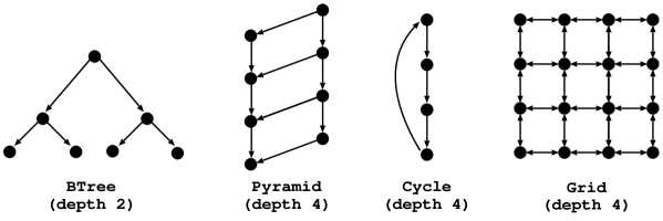
Figure 13: Edge configurations for the path benchmarks

The columns in Table 6 have the following meaning:

• calls: is the number of different calls to tabled subgoals. It corresponds to the number of paths in the subgoal tries.

• trie nodes: is the total number of trie nodes allocated in the corresponding subgoal/answer trie structures.

• trie depth: is the minimum/average/maximum number of trie node levels required to represent a path in the corresponding subgoal/answer trie structures. Trie structures with smaller average values are more amenable to contention, i.e., to have a higher number of synchronization points.

• unique: is the number of different tabled answers found. It corresponds to the number of paths in the answer tries.

• repeated: is the number of redundant tabled answers found.

• NS: is the average execution time, in seconds, of ten runs for 1 thread with the NS design.

Table 6: Characteristics of the benchmark programs

Bench	Tabled Subgoals				Tabled Answers				Time (sec)
	calls	trie nodes	trie depth		unique	repeated	trie nodes	trie depth	NS
Large Joins
Join2	1	6	5/5/5		2,476,099	0	2,613,660	5/5/5	2.85
Mondial	35	42	3/4/4		2,664	2,452,890	14,334	6/7/7	0.84
WordNet
Clusters	117,659	235,319	2/2/2		166,877	161,853	284,536	1/1/1	0.83
Holo	117,657	235,315	2/2/2		74,838	54	192,495	1/1/1	0.75
Hyper	117,657	235,315	2/2/2		698,472	8,658	816,129	1/1/1	1.42
Hypo	117,657	117,659	2/2/2		698,472	20,341	816,129	1/1/1	1.53
Mero	117,657	117,659	2/2/2		74,838	13	192,495	1/1/1	0.74
Tropo	117,657	235,315	2/2/2		472	0	118,129	1/1/1	0.66
Model Checking
IProto	1	6	5/5/5		134,361	385,423	1,554,896	4/51/67	2.70
Leader	1	5	4/4/4		1,728	574,786	41,788	15/80/97	3.51
Sieve	1	7	6/6/6		380	1,386,181	8,624	21/53/58	18.50
Path Left
BTree	1	3	2/2/2		1,966,082	0	2,031,618	2/2/2	1.53
Cycle	1	3	2/2/2		4,000,000	2,000	4,002,001	2/2/2	3.52
Grid	1	3	2/2/2		1,500,625	4,335,135	1,501,851	2/2/2	1.93
Pyramid	1	3	2/2/2		3,374,250	1,124,250	3,377,250	2/2/2	3.08
Path Right
BTree	131,071	262,143	2/2/2		3,801,094	0	3,997,700	1/2/2	2.33
Cycle	2,001	4,003	2/2/2		8,000,000	4,000	8,004,001	1/2/2	3.55
Grid	1,226	2,453	2/2/2		3,001,250	8,670,270	3,003,701	1/2/2	2.32
Pyramid	3,000	6,001	2/2/2		6,745,501	2,247,001	6,751,500	1/2/2	3.17

The Mondial benchmark, from the Large Joins set, and the three Model Checking benchmarks seem to be the benchmarks least amenable to contention since they are the ones that find less unique answers and that have the deepest trie structures. In this regard, the Path Left and Path Right sets correspond to the opposite case. They find a huge number of answers and have very shallow trie structures. On the other hand, the WordNet and Path Right sets have the benchmarks with the largest number of different subgoal calls, which can reduce the probability of contention because answers can be found for different subgoal calls and therefore be inserted with minimum overlap. On the opposite side are the Join2 benchmark, from the Large Joins set, and the Path Left benchmarks, which have only a single tabled subgoal call.

References

- Alba et al. (2002) Alba, E., Almeida, F., Blesa, M. J., Cabeza, J., Cotta, C., Díaz, M., Dorta, I., Gabarró, J., León, C., Luna, J., Moreno, L. M., Pablos, C., Petit, J., Rojas, A., and Xhafa, F. 2002. MALLBA: A Library of Skeletons for Combinatorial Optimisation (Research Note). In International Euro-Par Conference. Number 2400 in LNCS. Springer, 927–932.
- Ali and Karlsson (1990) Ali, K. and Karlsson, R. 1990. The Muse Approach to OR-Parallel Prolog. International Journal of Parallel Programming 19, 2, 129–162.
- Areias and Rocha (2011) Areias, M. and Rocha, R. 2011. On Combining Linear-Based Strategies for Tabled Evaluation of Logic Programs. Journal of Theory and Practice of Logic Programming, International Conference on Logic Programming, Special Issue 11, 4–5, 681–696.
- Areias and Rocha (2012a) Areias, M. and Rocha, R. 2012a. An Efficient and Scalable Memory Allocator for Multithreaded Tabled Evaluation of Logic Programs. In International Conference on Parallel and Distributed Systems. IEEE Computer Society, 636–643.
- Areias and Rocha (2012b) Areias, M. and Rocha, R. 2012b. Towards Multi-Threaded Local Tabling Using a Common Table Space. Journal of Theory and Practice of Logic Programming, International Conference on Logic Programming, Special Issue 12, 4 & 5, 427–443.
- Areias and Rocha (2013) Areias, M. and Rocha, R. 2013. Batched Evaluation of Linear Tabled Logic Programs. Journal of Computer Science and Information Systems, Special Issue on Advances in Model Driven Engineering, Languages and Agents 10, 4 (October), 1775–1797.
- Areias and Rocha (2014) Areias, M. and Rocha, R. 2014. On the Correctness and Efficiency of Lock-Free Expandable Tries for Tabled Logic Programs. In International Symposium on Practical Aspects of Declarative Languages, M. Flatt and H.-F. Guo, Eds. Number 8324 in LNCS. Springer, San Diego, California, USA, 168–183.
- Areias and Rocha (2015a) Areias, M. and Rocha, R. 2015a. Batched Evaluation of Full-Sharing Multithreaded Tabling. In Post-Proceedings of the 4th Symposium on Languages, Applications and Technologies. Number 563 in CCIS. Springer, 113–124.
- Areias and Rocha (2015b) Areias, M. and Rocha, R. 2015b. A lock-free hash trie design for concurrent tabled logic programs. International Journal of Parallel Programming, 1–21.
- Areias and Rocha (2017) Areias, M. and Rocha, R. 2017. On Scaling Dynamic Programming Problems with a Multithreaded Tabling System. Journal of Systems and Software 125, 417–426.
- Bagwell (2001) Bagwell, P. 2001. Ideal Hash Trees. Es Grands Champs 1195.
- Berger et al. (2000) Berger, E. D., McKinley, K. S., Blumofe, R. D., and Wilson, P. R. 2000. Hoard: A Scalable Memory Allocator for Multithreaded Applications. ACM SIGPLAN Notices 35, 11, 117–128.
- Blumofe et al. (1995) Blumofe, R. D., Joerg, C. F., Kuszmaul, B. C., Leiserson, C. E., Randall, K. H., and Zhou, Y. 1995. Cilk: An efficient multithreaded runtime system. SIGPLAN Not. 30, 8 (Aug.), 207–216.
- Carro and Hermenegildo (1999) Carro, M. and Hermenegildo, M. V. 1999. Concurrency in Prolog Using Threads and a Shared Database. In International Conference on Logic Programming. The MIT Press, 320–334.
- Chapman et al. (2008) Chapman, B., Jost, G., and van der Pas, R. 2008. Using OpenMP: Portable Shared Memory Parallel Programming. The MIT Press.
- Chen and Warren (1996) Chen, W. and Warren, D. S. 1996. Tabled Evaluation with Delaying for General Logic Programs. Journal of the ACM 43, 1, 20–74.
- Chico et al. (2008) Chico, P., Carro, M., Hermenegildo, M. V., Silva, C., and Rocha, R. 2008. An Improved Continuation Call-Based Implementation of Tabling. In International Symposium on Practical Aspects of Declarative Languages. Number 4902 in LNCS. Springer, 197–213.
- Costa et al. (2009) Costa, J., Raimundo, J., and Rocha, R. 2009. A Term-Based Global Trie for Tabled Logic Programs. In International Conference on Logic Programming. Number 5649 in LNCS. Springer, 205–219.
- Cruz and Rocha (2010) Cruz, F. and Rocha, R. 2010. Retroactive Subsumption-Based Tabled Evaluation of Logic Programs. In European Conference on Logics in Artificial Intelligence. Number 6341 in LNAI. Springer, 130–142.
- Desouter et al. (2015) Desouter, B., van Dooren, M., and Schrijvers, T. 2015. Tabling as a library with delimited control. Journal of Theory and Practice of Logic Programming 15, 4 & 5, 419–433.
- Evans (2006) Evans, J. 2006. A Scalable Concurrent malloc(3) Implementation for FreeBSD. In The Technical BSD Conference.
- Fonseca et al. (2009) Fonseca, N. A., Srinivasan, A., Silva, F. M. A., and Camacho, R. 2009. Parallel ILP for distributed-memory architectures. Machine Learning 74, 3, 257–279.
- Fredkin (1962) Fredkin, E. 1962. Trie Memory. Communications of the ACM 3, 490–499.
- Freire et al. (1996) Freire, J., Swift, T., and Warren, D. S. 1996. Beyond Depth-First: Improving Tabled Logic Programs through Alternative Scheduling Strategies. In International Symposium on Programming Language Implementation and Logic Programming. Number 1140 in LNCS. Springer, 243–258.
- (25) Ghemawat, S. and Menage, P. TCMalloc: Thread-Caching Malloc. Available: http://goog-perftools.sourceforge.net/doc/tcmalloc.html.
- Gidenstam et al. (2010) Gidenstam, A., Papatriantafilou, M., and Tsigas, P. 2010. NBmalloc: Allocating memory in a lock-free manner. Algorithmica 58, 2, 304–338.
- (27) Gloger, W. Ptmalloc. Available: http://www.malloc.de/en/.
- Guo and Gupta (2001) Guo, H.-F. and Gupta, G. 2001. A Simple Scheme for Implementing Tabled Logic Programming Systems Based on Dynamic Reordering of Alternatives. In International Conference on Logic Programming. Number 2237 in LNCS. Springer, 181–196.
- Gupta and Pontelli (1999) Gupta, G. and Pontelli, E. 1999. Stack Splitting: A Simple Technique for Implementing Or-parallelism on Distributed Machines. In International Conference on Logic Programming. The MIT Press, 290–304.
- Gupta et al. (2001) Gupta, G., Pontelli, E., Ali, K., Carlsson, M., and Hermenegildo, M. V. 2001. Parallel Execution of Prolog Programs: A Survey. ACM Transactions on Programming Languages and Systems 23, 4, 472–602.
- Herlihy and Wing (1987) Herlihy, M. and Wing, J. M. 1987. Axioms for Concurrent Objects. In ACM Symposium on Principles of Programming Languages. ACM, 13–26.
- Hermenegildo and Greene (1991) Hermenegildo, M. V. and Greene, K. 1991. The &-Prolog System: Exploiting Independent And-Parallelism. New Generation Computing 9, 3-4, 233–257.
- Herrmann and Lengauer (2000) Herrmann, C. A. and Lengauer, C. 2000. HDC: A Higher-Order Language for Divide-and-Conquer. Parallel Processing Letters 10, 2/3, 239–250.
- Johnson et al. (1999) Johnson, E., Ramakrishnan, C. R., Ramakrishnan, I. V., and Rao, P. 1999. A Space Efficient Engine for Subsumption-Based Tabled Evaluation of Logic Programs. In Fuji International Symposium on Functional and Logic Programming. Number 1722 in LNCS. Springer, 284–300.
- Knuth (1998) Knuth, D. E. 1998. The art of computer programming, volume 3: (2nd ed.) sorting and searching. Addison-Wesley Longman.
- Kumar (2002) Kumar, V. 2002. Introduction to Parallel Computing, 2nd ed. Addison-Wesley.
- Kumar et al. (1994) Kumar, V., Grama, A., Gupta, A., and Karypis, G. 1994. Introduction to Parallel Computing: Design and Analysis of Algorithms. Benjamin-Cummings Publishing Co., Inc.
- Liang et al. (2009) Liang, S., P.Fodor, Wan, H., and M.Kifer. 2009. OpenRuleBench: An Analysis of the Performance of Rule Engines. In Internacional World Wide Web Conference. ACM, 601–610.
- Loogen et al. (2005) Loogen, R., Ortega-Mallén, Y., and Peña-Marí, R. 2005. Parallel functional programming in Eden. Journal of Functional Programming 15, 3, 431–475.
- Lusk et al. (1988) Lusk, E., Butler, R., Disz, T., Olson, R., Overbeek, R., Stevens, R., Warren, D. H. D., Calderwood, A., Szeredi, P., Haridi, S., Brand, P., Carlsson, M., Ciepielewski, A., and Hausman, B. 1988. The Aurora Or-Parallel Prolog System. In International Conference on Fifth Generation Computer Systems. Institute for New Generation Computer Technology, 819–830.
- Marques and Swift (2008) Marques, R. and Swift, T. 2008. Concurrent and Local Evaluation of Normal Programs. In International Conference on Logic Programming. Number 5366 in LNCS. Springer, 206–222.
- Marques et al. (2010) Marques, R., Swift, T., and Cunha, J. C. 2010. A Simple and Efficient Implementation of Concurrent Local Tabling. In International Symposium on Practical Aspects of Declarative Languages. Number 5937 in LNCS. Springer, 264–278.
- Martello and Toth (1990) Martello, S. and Toth, P. 1990. Knapsack Problems: Algorithms and Computer Implementations. John Wiley and Sons.
- Masmano et al. (2006) Masmano, M., Ripoll, I., and Crespo, A. 2006. A comparison of memory allocators for real-time applications. In Proceedings of the 4th International Workshop on Java Technologies for Real-time and Embedded Systems. JTRES ’06. ACM, 68–76.
- Moura (2008) Moura, P. 2008. ISO/IEC DTR 13211–5:2007 Prolog Multi-threading Predicates.
- Peláez et al. (2007) Peláez, I., Almeida, F., and Suárez, F. 2007. DPSKEL: A Skeleton Based Tool for Parallel Dynamic Programming. In International Conference on Parallel Processing and Applied Mathematics. Number 4967 in LNCS. Springer, 1104–1113.
- Pontelli and Gupta (1997) Pontelli, E. and Gupta, G. 1997. Implementation Mechanisms for Dependent And-Parallelism. In International Conference on Logic Programming. The MIT Press, 123–137.
- Ramakrishnan et al. (1999) Ramakrishnan, I. V., Rao, P., Sagonas, K., Swift, T., and Warren, D. S. 1999. Efficient Access Mechanisms for Tabled Logic Programs. Journal of Logic Programming 38, 1, 31–54.
- Rao et al. (1996) Rao, P., Ramakrishnan, C. R., and Ramakrishnan, I. V. 1996. A Thread in Time Saves Tabling Time. In Joint International Conference and Symposium on Logic Programming. The MIT Press, 112–126.
- Reinders (2007) Reinders, J. 2007. Intel Threading Building Blocks, First ed. O’Reilly & Associates, Inc., Sebastopol, CA, USA.
- Rocha et al. (1999) Rocha, R., Silva, F., and Santos Costa, V. 1999. Or-Parallelism within Tabling. In International Workshop on Practical Aspects of Declarative Languages. Number 1551 in LNCS. Springer, 137–151.
- Rocha et al. (2001) Rocha, R., Silva, F., and Santos Costa, V. 2001. On a Tabling Engine That Can Exploit Or-Parallelism. In International Conference on Logic Programming. Number 2237 in LNCS. Springer, 43–58.
- Rocha et al. (2005) Rocha, R., Silva, F., and Santos Costa, V. 2005. On applying or-parallelism and tabling to logic programs. Theory and Practice of Logic Programming 5, 1 & 2, 161–205.
- Sagonas and Swift (1998) Sagonas, K. and Swift, T. 1998. An Abstract Machine for Tabled Execution of Fixed-Order Stratified Logic Programs. ACM Transactions on Programming Languages and Systems 20, 3, 586–634.
- Saha (2006) Saha, D. 2006. Incremental Evaluation of Tabled Logic Programs. Ph.D. thesis, Department of Computer Science, State University of New York.
- Santos and Rocha (2013) Santos, J. and Rocha, R. 2013. On the Efficient Implementation of Mode-Directed Tabling. In International Symposium on Practical Aspects of Declarative Languages. Number 7752 in LNCS. Springer, 141–156.
- Santos Costa et al. (2012) Santos Costa, V., Rocha, R., and Damas, L. 2012. The YAP Prolog System. Journal of Theory and Practice of Logic Programming 12, 1 & 2, 5–34.
- Santos Costa et al. (1991) Santos Costa, V., Warren, D. H. D., and Yang, R. 1991. Andorra-I: A Parallel Prolog System that Transparently Exploits both And- and Or-Parallelism. In ACM Symposium on Principles and Practice of Parallel Programming. ACM, 83–93.
- Shen (1992) Shen, K. 1992. Exploiting Dependent And-parallelism in Prolog: The Dynamic Dependent And-Parallel Scheme (DDAS). In Joint International Conference and Symposium on Logic Programming. The MIT Press, 717–731.
- Somogyi and Sagonas (2006) Somogyi, Z. and Sagonas, K. 2006. Tabling in Mercury: Design and Implementation. In International Symposium on Practical Aspects of Declarative Languages. Number 3819 in LNCS. Springer, 150–167.
- Stivala et al. (2010) Stivala, A., Stuckey, P., de la Banda, M. G., Hermenegildo, M., and Wirth, A. 2010. Lock-Free Parallel Dynamic Programming. Journal of Parallel and Distributed Computing 70, 8, 839–848.
- Swift and Warren (2012) Swift, T. and Warren, D. S. 2012. XSB: Extending Prolog with Tabled Logic Programming. Theory and Practice of Logic Programming 12, 1 & 2, 157–187.
- Tenenbaum et al. (1990) Tenenbaum, A. M., Langsam, Y., and Augenstein, M. J. 1990. Data Structures Using C. Prentice Hall.
- Zhou (2012) Zhou, N.-F. 2012. The Language Features and Architecture of B-Prolog. Journal of Theory and Practice of Logic Programming 12, 1 & 2, 189–218.
- Zhou et al. (2015) Zhou, N.-F., Kjellerstrand, H., and Fruhman, J. 2015. Constraint Solving and Planning with Picat. Springer.