Emergence of correlations in the process of thermalization of interacting bosons

Abstract

We address the question of the relevance of thermalization to the increase of correlations in the quench dynamics of an isolated system with a finite number of interacting bosons. Specifically, we study how, in the process of thermalization, the correlations between occupation numbers increase in time resulting in the emergence of the Bose-Einstein distribution. We show, both analytically and numerically, that before saturation the two-point correlation function increases quadratically in time. This time dependence is at variance with the exponential increase of the number of principal components of the wave function, recently discovered and explained in Ref.BIS18 . We also demonstrate that the out-of-time-order correlator (OTOC) increases algebraically in time but not exponentially as predicted in many publications. Our results, that can be confirmed experimentally in traps with interacting bosons, may be also relevant to the problem of black hole scrambling.

Introduction - In recent years the problem of thermalization in closed systems of interacting fermions and bosons has attracted much attention (see, for example, Refs.reviews ; BISZ16 ). An increase of interest to this problem is due to remarkable experimental achievements exp and various theoretical predictions zele ; flam ; deutsch . Although the term thermalization is not uniquely defined, it is widely used in many-body physics. One of the basic statistical properties of many-body systems is either the Bose-Einstein (BE) or Fermi-Dirac (FD) distribution that emerge in the thermodynamic limit due to the combinatorics and without inter-particle interaction. As for finite isolated systems, the mechanism for the onset of BE and FD distributions is the chaotic structure of many-body eigenstates zele ; flam ; BGIC98 ; BCIC02 ; BISZ16 ; BMI17 . In this case, the interaction between particles plays a crucial role: the fewer the particles the stronger the inter-particle interaction has to be for the emergence of the statistical properties.

To date it is understood that the validity of statistical mechanics can be justified not only by averaging over a number of eigenstates with close energies, but also with the use of a single eigenstate if the latter consists of many uncorrelated components in the physically chosen basis. Specifically, it was shown that BE and FD distributions emerge also on the level of individual eigenstates if they are strongly chaotic BGIC98 ; GGF99 ; BMI17 . The most intriguing point here is that both distributions appear even if the number of particles is small; this happens due to the fast growth of the number of components in many-body eigenstates in dependence on the number of particles.

Unlike the onset of BE and FD distributions emerging from single stationary eigenstates, in this Letter we address a new problem concerning the onset of the BE distribution in the evolution of a system with few interacting bosons. Our specific interest is to study how the conventional BE distribution emerges in time and how this fact is related to the somewhat different problem of the increase of correlations in the process of relaxation of a system to a steady-state distribution. The latter problem is now a hot topic in literature in view of various applications, such as the evolution of systems with cold atoms, as well as in application to the problem of scrambling in black holes (see M18 and references therein).

In our study we consider the quench dynamics described by the Hamiltonian $H=H_{0}+V$ where $H_{0}$ represents the non-interacting bosons and the interaction is fully embedded into $V$ belonging to the ensemble of two-body random interacting (TBRI) matrices. In this way, by exciting initially a single many-body state of $H_{0}$ we explore the evolution of wave packets in the Fock space. Recently, it was discovered that for the model parameters for which the many-body eigenstates of $H$ are strongly chaotic, the effective number of components $N_{pc}$ in the wave function increases exponentially in time, before the saturation which is due to the finite number of particles BIS18 . This time dependence was explained with the use of a phenomenological model that allowed to obtain simple analytical expressions for the rate of exponential increase of $N_{pc}$ and for its saturation value.

Below, in connection with the results reported in BMI17 ; BIS18 we show, both analytically and numerically, that the onset of the BE distribution in the TBRI matrix model occurs on the time scale on which the number of components in many-body eigenstates increases exponentially in time. In order to quantify the onset of the BE distribution we have studied the correlations between occupation numbers by exploring both the two- and four- point correlators. The latter is just the well known OTOC correlator widely discussed in literature OTOC . Specifically, it was predicted that for strongly chaotic systems OTOC should manifest an exponential time-dependence before saturation. One of our main findings is that actually both correlators increase algebraically in time and not exponentially. This result is quite unexpected, as compared with the exponential increase of the number of principal components $N_{pc}$ in the wave packet. Our analytical results are fully confirmed by extensive numerical data.

The model - The system consists of $N$ identical bosons occupying $M$ single-particle levels specified by random energies $\epsilon_{s}$ with mean spacing, $\langle\epsilon_{s}-\epsilon_{s-1}\rangle=1$. The Hamiltonian $H=H_{0}+V$ reads ($\hbar=1$),

$$H=\sum\epsilon_{s}\,a^{\dagger}_{s}a_{s}+\sum V_{s_{1}s_{2}s_{3}s_{4}}\,a^{\dagger}_{s_{1}}a^{\dagger}_{s_{2}}a_{s_{3}}a_{s_{4}}$$ (1)

where the two-body matrix elements $V_{s_{1}s_{2}s_{3}s_{4}}$ are random Gaussian entries with zero mean and variance $V^{2}$. The dimension of the Hilbert space generated by the many-particle basis states is ${N_{H}}=(N+M-1)!/N!(M-1)!$ Here we consider $N=6$ particles in $M=11$ levels (dilute limit, $N\leq M$) for which $N_{H}=8008$. Two-body random matrices (1) were introduced in TBRI ; brody and extensively studied for fermions flam ; alt and bosons bosons .

The eigenstates $\left|\alpha\,\right\rangle=\sum_{k}C_{k}^{(\alpha)}\left|k\,\right\rangle$ of $H$ can be written in terms of the basis states $|k\rangle=a^{\dagger}_{k_{1}}...a^{\dagger}_{k_{N}}|0\rangle$ of $H_{0}$, where

$$H|\alpha\rangle=E^{\alpha}|\alpha\rangle;\quad H_{0}|k\rangle=E^{0}_{k}|k\rangle.$$ (2)

An eigenstate $\left|\alpha\,\right\rangle$ of the total Hamiltonian is called chaotic when its number $N_{pc}$ of principal components $C_{k}^{\alpha}$ is sufficiently large and $C_{k}^{\alpha}$ can be considered as random and non-correlated ones. Note that since the system is isolated and the perturbation $V$ is finite, the eigenstates can fill only a part of the unperturbed basis BISZ16 determined by the perturbation $V$. Specifically, the energy region which is occupied by the eigenstates is restricted by the width of the so-called energy shell chirikov . The partial filling of the energy shell by an eigenstate can be associated with the many-body localization in the energy representation. Contrary, when an eigenstate fills completely the energy shell, we are in presence of maximal quantum chaos, and the BE distribution emerges on the level of individual eigenstates BGIC98 ; GGF99 ; BMI17 . This happens when the interaction $V$ is sufficiently large, $V>V_{cr}$, to provide strong quantum chaos. In what follows we will consider the situation when the latter condition is fulfilled.

Dynamics in Fock space - In contrast with the previous studies BMI17 , focused on the thermal properties of individual many-body eigenstates, here we consider the dynamics of the model (1) by exploring two different time scales, before and after the relaxation to a steady state. Specifically, we study the quench dynamics starting from a single many-body state $\left|k_{0}\,\right\rangle$ of the unperturbed Hamiltonian $H_{0}$, after switching on the interaction $V$. Given the evolved wave function $\left|\psi(t)\,\right\rangle=e^{-iHt}\left|k_{0}\,\right\rangle$ one can express the probability $P_{k}(t)=|\left\langle k\,\right|\psi(t)\rangle|^{2}$ to find the system at time $t$ in any unperturbed state $\left|k\,\right\rangle$ as follows,

$$P_{k}(t)=\sum_{\alpha,\beta}C_{k_{0}}^{\alpha\ast}C_{k}^{\alpha}C_{k_{0}}^{\beta}C_{k}^{\beta\ast}e^{-i(E^{\beta}-E^{\alpha})t}\equiv P_{k,k_{0}}^{d}+P_{k,k_{0}}^{f}(t),$$ (3)

where $P_{k,k_{0}}^{d}=\sum_{\alpha}|C_{k_{0}}^{\alpha}|^{2}|C_{k}^{\alpha}|^{2}$ and $P_{k,k_{0}}^{f}(t)$ are the time-independent and time-fluctuating parts, respectively. With this expression, one can analyze the number of principal components,

$$N_{pc}(t)=\left\{\sum\limits_{k}\left[P_{k,k_{0}}^{d}+P_{k,k_{0}}^{f}(t)\right]^{2}\right\}^{-1},$$ (4)

known as the participation ratio. Taking the long-time average, $P_{k,k_{0}}^{f}(t)$ cancels out and only the diagonal part $P_{k}^{d}$ survives. As is shown in BIS18 the number $N_{pc}(t)$ of principal components in the wave packets increases exponentially fast in time, $N_{pc}(t)\sim\exp(2\Gamma t)$ up to some saturation time $t_{s}$. The rate of the exponential growth is defined by the width $\Gamma$ of the local density of states (LDOS),

$$F_{k_{0}}(E)=\sum_{\alpha}|C_{k_{0}}^{\alpha}|^{2}\delta(E-E^{\alpha}),$$

obtained by projecting the initial state $\left|k_{0}\,\right\rangle$ onto the energy eigenstates. In nuclear physics it is known as strength function and it describes the relaxation of excited heavy nuclei bohr . Concerning the saturation time $t_{s}$, it was found BIS18 to be proportional to the number of particles, $t_{s}\approx N/\Gamma$. This time should be treated as the time after which one can speak of a complete thermalization occurring in a system. The exponential increase of $N_{pc}(t)$ is shown in SM , together with the analytical estimates obtained in Ref. BIS18 .

Figure 1: (Color online) Upper panels: Probability $P_{k}(t)$ at different times $t$ in the unperturbed basis $|k\rangle$. Low panels show $n_{s}(t)$ versus the single-particle energies $\epsilon_{s}$. In panel (d) the envelope of the stationary distribution is shown by a black curve. Initial state is $\Psi_{0}=|10104000000\rangle$ where integer numbers are numbers of bosons occupying the $s$-level. Dynamics is shown for $N=6,M=11$ and $V=0.4$. For this value of $V$ the eigenstates are strongly chaotic BMI17 .

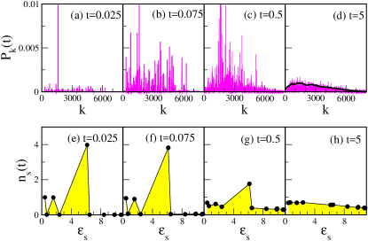
Onset of Bose-Einstein distribution - The time-dependent occupation number distribution (OND) is defined as follows,

$$n_{s}(t)=\left\langle\psi(t)\,\right|\hat{n}_{s}\left|\psi(t)\,\right\rangle=\sum_{k}n_{s}^{k}|\langle k|\psi(t)\rangle|^{2}.$$ (5)

It gives the average number of particles in the single-particle energy level $\epsilon_{s}$ at the time $t$. Here we took into account that $\left\langle k\,\right|\hat{n}_{s}\left|k^{\prime}\,\right\rangle=n_{s}^{k}\,\delta_{k,k^{\prime}}$ where $n_{s}^{k}=0,...,N$. The evolution of $n_{s}(t)$ in comparison with the wave packet dynamics $P_{k}(t)$ is shown in Fig 1(e)-(h). This figure demonstrates that when the packet fully occupies the energy shell, the occupation numbers are relaxed to the steady-state distribution.

Expanding $e^{-iHt}$ at second order one gets the time dependence for $n_{s}(t)$ at small times,

$$|\langle k|e^{-iHt}|k_{0}\rangle|^{2}\simeq\delta_{k,k_{0}}+t^{2}\left[H_{k,k_{0}}^{2}-\delta_{k_{0},k_{0}}(H^{2})_{k,k_{0}}\right]+o(t^{4})$$ (6)

which results in the following estimate,

$$n_{s}(t)\simeq n_{s}^{k_{0}}+t^{2}\sum_{k\neq k_{0}}(n_{s}^{k_{0}}-n_{s}^{k})H_{k,k_{0}}^{2}+o(t^{4})$$ (7)

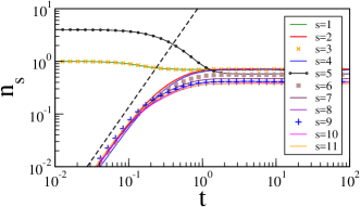
One can see in Fig. 2 that for single-particle $s-$levels which are not initially occupied by particles, $n_{s}(t)$ grows quadratically in time. As for the saturation values $\overline{n_{s}}$ after the relaxation time $t_{s}$, they can be also obtained analytically by performing an infinite time average,

$$\overline{n_{s}}=\sum_{k}n_{s}^{k}\overline{|\langle k|\psi(t)\rangle|^{2}}=\sum_{k}n_{s}^{k}P_{k,k_{0}}^{d}\ .$$ (8)

In order to claim that after relaxation the OND is statistically described by a BE distribution, one has to be sure that the fluctuations of $n_{s}$ follow the standard requirements of statistical mechanics. In view of this very point, we have thoroughly analyzed both “classical” and “quantum” fluctuations. Concerning the former, they can be analyzed by the search of the time dependence of $n_{s}(t)$ with respect to their asymptotic values reached after relaxation. According to the statistical mechanics, a) the fluctuations have to be small as compared to the mean values, and b) fluctuations should be Gaussian. Our numerical analysis of the fluctuations, see SM , has shown that the relative fluctuations $\Delta n_{s}/\langle n_{s}\rangle$ are Gaussian distributed and decreasing as $1/\sqrt{\overline{N}_{pc}}$ (infinite time average of $N_{pc}(t)$) instead of $1/\sqrt{N}$ (number of particles). This remarkable result shows that for systems having few chaotic interacting particles the number of principal components $\overline{N}_{pc}$ in the wave packet plays the same role as the number of particles $N$ in ordinary statistical mechanics. A more intriguing point concerns quantum fluctuations. It is a textbook result huang that BE statistics is characterized by relative quantum fluctuations $\delta n_{s}^{2}/n_{s}^{2}=1+1/n_{s}$, where $\delta n_{s}^{2}=\overline{n^{2}}_{s}-\overline{n}_{s}^{2}$ with the overbar standing for the infinite time-average, see Eq. (8). Once again we checked that, provided the time-dependent wave function is chaotic, fluctuations follow the predictions of standard statistical mechanics (for details see SM ). This should be considered as an additional proof of the statistical character of the evolution of the system after the relaxation.

Figure 2: Evolution of the averaged $n_{s}(t)$ for all $s=1,...,M$. Dashed line is the predicted $t^{2}$ behavior (7) characteristic of the perturbative regime. Initial state is $\Psi_{0}=|10104000000\rangle$. Here $N=6,M=11$ and $V=0.4$ as in Fig.1. An average over 10 realizations of the random potential has been used.

Two-point correlation function - Let us now study how the onset of the BE distribution is manifested by the emergence of correlations between occupation numbers. First, we start with the two-point correlation function ${C}_{s,s+1}(t)$ between neighboring occupation numbers,

$${C}_{s,s+1}(t)=\langle k_{0}|[\hat{n}_{s}(t)-\hat{n}_{s}][\hat{n}_{s+1}(t)-\hat{n}_{s+1}]|k_{0}\rangle.$$ (9)

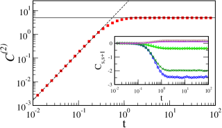
Initially the correlations are absent, ${C}_{s,s+1}(0)=0$, however, they appear in time. The time-dependence of ${C}_{s,s+1}(t)$ is shown in Fig. 3 for all $s=1,..,M-1$. As one can see, there is a clear relaxation to steady-state values after the critical time $t_{s}$. The negative or positive sign of the asymptotic correlations is related to the particular choice of the initial state.

It is also instructive to introduce the global correlator ${\cal C}^{(2)}$ which is the sum of the correlators between all neighboring single-particle energy levels $\epsilon_{s}$ and $\epsilon_{s+1}$,

$${\cal C}^{(2)}(t)=|\sum_{s=1}^{M-1}C_{s,s+1}(t)|.$$ (10)

This correlator is independent of the specific $s$ level and it can be used as a global measure of correlations between occupation numbers of nearest single-particle energy levels. Performing an expansion on a small time scale it is possible to show that

$${\cal C}^{(2)}(t)\simeq t^{2}|\sum_{s=1}^{M-1}\sum_{r=s+1}^{M}\sum_{k}H_{k,k_{0}}^{2}W_{k,k_{0}}^{sr}|+o(t^{4})$$ (11)

with $W_{k,k_{0}}^{sr}=[n_{s}^{k}n_{r}^{k}+n_{s}^{k_{0}}n_{r}^{k_{0}}-n_{s}^{k_{0}}n_{r}^{k}-n_{s}^{k}n_{r}^{k_{0}}]$. As one can see, Eq. (11) does not contain eigenvalues and eigenfunctions. This means that in order to get the initial spread of the correlator, there is no need to diagonalize the Hamiltonian. Concerning the saturation value, it can be obtained by performing the time average for $t\geq t_{s}$ (see SM ),

$$\overline{{\cal C}^{(2)}}=|\sum_{s=1}^{M-1}\sum_{r=s+1}^{M}\sum_{k}P_{k,k_{0}}^{d}W_{k,k_{0}}^{sr}|.$$ (12)

The time evolution for ${\cal C}^{(2)}(t)$ is shown in Fig.3, together with the analytical predictions. The correspondence between numerical data and analytical predictions is impressive. Thus, the dynamics of ${\cal C}^{(2)}(t)$ is fully described by the analytical expressions (11) and (12).

Figure 3: Global two-point correlation function ${\cal C}^{(2)}(t)$ (red squares). Dashed line is given by Eq. (11). Horizontal line corresponds to Eq. (12). The initial state and parameters are the same as in Fig.2. The average over $10$ realizations of the random potential was used. Inset: Correlation function $C_{s,s+1}(t)$ for all $s=1,...,M-1$.

Four-point correlation function (OTOC) - Now let us study the four-point correlator between nearest single-particle energy levels,

$${\cal O}_{s,s+1}(t)=\langle k_{0}|[\hat{n}_{s}(t),\hat{n}_{s+1}(0)]|^{2}|k_{0}\rangle.$$ (13)

This correlator, also known as OTOC, has been recently introduced in the frame of the SYK model SYK and widely discussed in view of various physical applications (see e.g. OTOC ).

After some algebra SM , one can obtain that the correlator ${\cal O}_{s,s+1}(t)$ increases in time quadratically on a small time scale, whose validity defines the perturbative regime,

$${\cal O}_{s,s+1}(t)\simeq t^{2}\sum_{k\neq k_{0}}H_{k,k_{0}}^{2}\left(n_{s}^{k}-n_{s}^{k_{0}}\right)^{2}\left(n_{s+1}^{k}-n_{s+1}^{k_{0}}\right)^{2}.$$ (14)

In the same way, by performing an infinite time-average, we can obtain the steady state value $\overline{{\cal O}_{s,s+1}}$,

$$\begin{array}[]{lll}&\overline{{\cal O}_{s,s+1}}=\sum_{k}\left(n_{s+1}^{k}-n_{s+1}^{k_{0}}\right)^{2}\left\{\left[\sum_{\alpha}C_{k}^{\alpha}C_{k_{0}}^{\alpha}{\cal N}_{s}^{\alpha,\alpha}\right]^{2}+\right.\\ &\left.\sum_{\alpha\neq\beta}|C_{k}^{\alpha}|^{2}|C_{k_{0}}^{\beta}|^{2}\left({\cal N}_{s}^{\alpha,\beta}\right)^{2}\right\}\end{array}$$ (15)

with ${\cal N}_{s}^{\alpha,\beta}=\sum_{k}C_{k}^{\alpha}C_{k}^{\beta}n_{s}^{k}$.

Figure 4: Evolution of the four-point correlator ${\cal O}_{s,s+1}(t)$ for $s=5$. Dashed line is the analytical prediction (14). Horizontal line corresponds to Eq. (15). Dotted line is the fit for $t>0.07$ (outside perturbative regime), giving the $t^{2.5}$ dependence. Initial state is $\Psi_{0}=|00006000000\rangle$ and $N=6,M=11,V=0.4$.

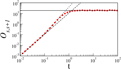
Numerical data for ${\cal O}_{s,s+1}(t)$ are shown in Fig. 4 together with the expressions (14) and (15). Our results demonstrate that while in the perturbative regime the growth is indeed quadratic, a time window can be found where the correlator increases approximately as $t^{2.5}$, before the saturation. This occurs at variance with the behavior of the two-point correlator for which only the quadratic regime before saturation is seen and with $N_{pc}$ which grows exponentially in time.

Conclusion and discussion - In this Letter we address the question of how the conventional Bose-Einstein distribution emerges in an isolated system with a finite number of interacting bosons. Since this process is accompanied by an increase of strong correlations between occupation numbers $n_{s}(t)$, the large part of our study is devoted to the details of the time dependence of these correlations.

For our analysis we have used the well known model (1) describing bosons interacting to each other via two-body random matrix elements. By exploring the quench dynamics, we show that the BE distribution emerges on the same time scale $t_{s}$ on which the number of principal components in the wave function increases exponentially in time in the Fock spaceBIS18 . This time scale $t_{s}$ is proportional to the number $N$ of bosons and defines the time after which one can speak of a complete thermalization in the system.

In order to confirm the true statistical behavior of the occupation numbers, we have carefully studied the fluctuations of $n_{s}(t)$ after the relaxation. In accordance with the standard statistical mechanics our data manifest that the fluctuations are of the Gaussian type, and that they are small compared to the mean values of $n_{s}(t)$. It was also shown that relative quantum fluctuations, $\delta n_{s}^{2}/n_{s}^{2}$, are also in agreement with the Bose statistics (see huang ).

In order to reveal how the process of thermalization is related to the onset of correlations, we have studied, both analytically and numerically, two correlators. One is the standard two-point correlator between nearest occupation numbers $n_{s}$ and $n_{s+1}$ and the other is the out-of-time order correlator (OTOC) recently discussed in literature. We have found that the two-point correlator increases in time quadratically before the saturation. As for the OTOC, initially, it also increases quadratically, however, before saturation our numerical data demonstrate the dependence $\sim t^{2.5}$ at variance with the quadratic increase predicted analytically. This result contradicts the prediction that the OTOC typically increases exponentially on some time scale OTOC .

Our results show how the information initially encoded in a local unperturbed state, spreads over the whole system and transforms onto global correlations specified by the BE distribution of occupation numbers. Although the dynamics is completely reversible due to the unitarity of the evolution operator, it is practically impossible to extract the information about the initial state, by measuring the correlations between the components of the wave function. Indeed the full information about the initial state can be extracted only if there is an additional complete knowledge of the random operator $V$ . Thus one can indeed speak of the loss of information due to scrambling. The process of this loss is accompanied by the emergence of global (thermodynamical) correlations, as demonstrated by the data reported in this Letter.

We hope that our study can help to understand the relation between thermalization and scrambling from one side, and the onset of correlations in the evolution of chaotic systems from the other one. Since the TBRI matrix model (1) has been proved to manifest generic statistical properties occurring in realistic physical systems (see, for example, lieb ), the obtained results can be confirmed experimentally by studying interacting bosons in optical traps. Our results may be also important in view of the problem of black hole scrambling, see M18 and references therein.

Acknowledgements.– We acknowledge financial support from VIEP-BUAP Grant No. IZF-EXC16-G (FMI) and Iniziativa Specifica INFN-DynSysMath (FB).

Supplemental Material for : Emergence of correlations in the process of thermalization of interacting bosons

Fausto Borgonovi Felix M. Izrailev

I Dynamics

Let us consider initially an unperturbed many-body state of $H_{0}$,

$$\left|\psi(0)\,\right\rangle=\left|k_{0}\,\right\rangle=\sum_{\alpha}C_{k_{0}}^{\alpha}\left|\alpha\,\right\rangle\ ,$$ (16)

whose evolution under the Hamiltonian $H=H_{0}+V$ is given by

$$\langle k|\psi(t)\rangle=\langle k|e^{-iHt}|\psi(0)\rangle=\langle k|e^{-iHt}|k_{0}\rangle=\sum_{\alpha}C_{k_{0}}^{\alpha}C_{k}^{\alpha}e^{-iE^{\alpha}t},$$ (17)

(note that all $C_{k}^{\alpha}$ are real numbers). The probability to be in the unperturbed many-body state $\left|k\,\right\rangle$ is

$$P_{k}(t)=|\langle k|\psi(t)\rangle|^{2}=\sum_{\alpha,\beta}C_{k_{0}}^{\alpha}C_{k}^{\alpha}C_{k_{0}}^{\beta}C_{k}^{\beta}e^{-i(E^{\beta}-E^{\alpha})t}\ ,$$ (18)

which can be written as a diagonal (time independent) plus a fluctuating (time-dependent) part,

$$P_{k}(t)=\sum_{\alpha}|C_{k_{0}}^{\alpha}|^{2}|C_{k}^{\alpha}|^{2}+\sum_{\alpha\neq\beta}C_{k_{0}}^{\alpha}C_{k}^{\alpha}C_{k_{0}}^{\beta}C_{k}^{\beta}e^{-i(E^{\beta}-E^{\alpha})t}\equiv P_{k,k_{0}}^{d}+P_{k,k_{0}}^{f}(t).$$ (19)

Let us now define the long-time average of an observable $A(t)$ as

$$\overline{A}=\lim_{T\to\infty}\ \frac{1}{T}\int_{0}^{T}\ dt\ A(t).\$$ (20)

It is clear that for a non-degenerate spectrum $\overline{P_{k,k_{0}}^{f}(t)}=0$ so that,

$$\overline{P_{k}(t)}=\sum_{\alpha}|C_{k_{0}}^{\alpha}|^{2}|C_{k}^{\alpha}|^{2}=P_{k,k_{0}}^{d}\ .$$ (21)

Figure 5: (a) Number $N_{pc}(t)$ of principal components in time (red circles). Dashed line is the exponential growth with the rate $2\Gamma$ where $\Gamma\approx 2.8$ is the width of the LDOS found numerically from the decay of survival probability (for details see bis18 ). Horizontal line is the estimate (23). Inset : Initial quadratic dependence $N_{pc}(t)\propto t^{2}$. Initially all bosons are placed on the $5$-th single-particle level so that $\left|\psi_{0}\,\right\rangle=\left|k_{0}\,\right\rangle=|00006000000\rangle$. (b) Orange dots represent the long-time average number of principal components as a function of the energy $E_{k}^{0}$ of the initial many-body state. Black curve is a Gaussian fit. Here is $N=6$, $M=11$, $V=0.4$.

I.1 Number of Principal Components

The long-time average for the number of principal components can be computed as follows. Let us start from its definition,

$$[N_{pc}(t)]^{-1}=\sum_{k}|\langle k|\psi(t)\rangle|^{4}\equiv\sum_{k}[P_{k,k_{0}}^{d}+P_{k,k_{0}}^{f}(t)]^{2}.$$ (22)

Taking the infinite-time average we have

$$[\overline{N}_{pc}]^{-1}=\sum_{k}(P_{k,k_{0}}^{d})^{2}+\overline{[P_{k,k_{0}}^{f}(t)]^{2}}.$$ (23)

The second term in the r.h.s. of Eq. (23) can be computed exactly,

$$\overline{[P_{k,k_{0}}^{f}(t)]^{2}}=(P_{k,k_{0}}^{d})^{2}-\sum_{\alpha}\left|C_{k_{0}}^{\alpha}\right|^{4}|C_{k}^{\alpha}|^{4}$$ (24)

so that the long-time average for the number of principal components is given by,

$$\overline{N}_{pc}=\left[2\sum_{k}(P_{k,k_{0}}^{d})^{2}-\sum_{\alpha}|C_{k_{0}}^{\alpha}|^{4}\sum_{k}|C_{k}^{\alpha}|^{4}\right]^{-1}.$$ (25)

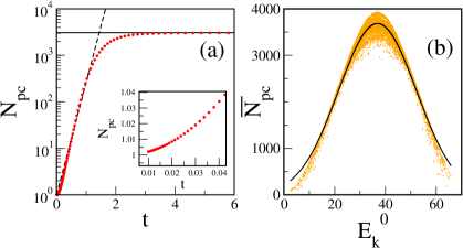
This expression determines the asymptotic value reached by $N_{pc}(t)$ after relaxation. It is shown in Fig. 5(a) as a horizontal line. In the same figure we can identify three different regimes : a perturbative one for short time $t\ll 1/\Gamma$ where $N_{pc}(t)$ grows quadratically (see inset in Fig. 5 (a)); a second one characterized by the exponential growth, $N_{pc}(t)\simeq\exp(2\Gamma t)$ for $1/\Gamma\lesssim t\lesssim N/\Gamma$, and a third one (saturation after relaxation) where $N_{pc}(t)\simeq\overline{N}_{pc}$ for $t>N/\Gamma$ (for details see bis18 ).

Another important information is how the stationary value $\overline{N}_{pc}$ depends on the initial state. In Fig. 5(b) we show $\overline{N}_{pc}$ as a function of the unperturbed energy $E_{k}^{0}$ of the initial many-body state $\left|k_{0}\,\right\rangle$. As one can see it is quite well approximated (excluding the tails) by a Gaussian shape (see black full curve).

I.2 Single-particle Occupation Numbers

Time dependent single-particle occupation numbers are defined as,

$$n_{s}(t)=\left\langle\psi(t)\,\right|\hat{n}_{s}\left|\psi(t)\,\right\rangle=\sum_{k}n_{s}^{k}|\langle k|\psi(t)\rangle|^{2}.$$ (26)

Performing the infinite time average one obtains for the first two moments,

$$\begin{array}[]{lll}\overline{n_{s}}&=\sum_{k}n_{s}^{k}\overline{|\langle k|\psi(t)\rangle|^{2}}=\sum_{k}n_{s}^{k}P_{k,k_{0}}^{d}\\ &\\ \overline{n_{s}^{2}}&=\sum_{k}(n_{s}^{k})^{2}\overline{|\langle k|\psi(t)\rangle|^{2}}=\sum_{k}(n_{s}^{k})^{2}P_{k,k_{0}}^{d}\ .\end{array}$$ (27)

and from that

$$\delta n_{s}^{2}(k_{0})=\sum_{k}(n_{s}^{k})^{2}P_{k,k_{0}}^{d}-\left(\sum_{k}n_{s}^{k}P_{k,k_{0}}^{d}\right)^{2},$$ (28)

where the dependence on $k_{0}$ has been explicitly indicated in Eq. (28).

Figure 6: Single-particle occupation numbers as a function of time after relaxation. Different colors stand for different $s=1,..,M$. Initial state is, in second quantized form, $\left|\psi_{0}\,\right\rangle=|00006000000\rangle$. Here is $N=6,M=11,V=0.4$.

I.3 Two-point Correlation Function

First of all let us notice that the number operator $\hat{n}_{s}$ giving the number of particles in the single-particle energy level $\epsilon_{s}$ is diagonal in the unperturbed many-body basis, i.e.

$$\left\langle k\,\right|\hat{n}_{s}\left|k^{\prime}\,\right\rangle=\delta_{k,k^{\prime}}n_{s}^{k}.$$ (29)

Concerning the global two-point correlation function one has, starting from the initial state $\left|k_{0}\,\right\rangle$,

$$\begin{array}[]{lll}{\cal C}^{(2)}(t)&=\sum_{s=1}^{M-1}\langle k_{0}|[\hat{n}_{s}(t)-\hat{n}_{s}][\hat{n}_{s+1}(t)-\hat{n}_{s+1}]|k_{0}\rangle\\ &\\ &=\sum_{s=1}^{M-1}\langle k_{0}|\hat{n}_{s}(t)\hat{n}_{s+1}(t)|k_{0}\rangle-n_{s}^{k_{0}}\langle k_{0}|n_{s+1}(t)|k_{0}\rangle-n_{s+1}^{k_{0}}\langle k_{0}|n_{s}(t)|k_{0}\rangle+n_{s}^{k_{0}}n_{s+1}^{k_{0}}\\ &\\ &=\sum_{s=1}^{M-1}\sum_{k}|\langle k|\psi(t)\rangle|^{2}[n_{s}^{k}n_{r}^{k}+n_{s}^{k_{0}}n_{r}^{k_{0}}-n_{s}^{k_{0}}n_{r}^{k}-n_{s}^{k}n_{r}^{k_{0}}]\equiv\sum_{s=1}^{M-1}\sum_{k}|\langle k|\psi(t)\rangle|^{2}W_{k,k_{0}}^{sr},\end{array}$$ (30)

where $\hat{n}_{s}(t)=e^{iHt}\hat{n}_{s}e^{-iHt}$. In Eq. (30) we have defined

$$W_{k,k_{0}}^{sr}=[n_{s}^{k}n_{r}^{k}+n_{s}^{k_{0}}n_{r}^{k_{0}}-n_{s}^{k_{0}}n_{r}^{k}-n_{s}^{k}n_{r}^{k_{0}}].$$ (31)

The long-time average is thus given by,

$$\overline{{\cal C}^{(2)}}=\sum_{s=1}^{M-1}\sum_{k}P_{k,k_{0}}^{d}W_{k,k_{0}}^{sr}.$$ (32)

I.4 Four-point Correlation Function

Let us obtain the long-time estimate for the four-point correlation function (OTOC):

$${\cal O}_{s,s+1}(t)=\langle k_{0}|[\hat{n}_{s}(t),\hat{n}_{s+1}(0)]|^{2}|k_{0}\rangle.$$ (33)

From the definition it is clear that ${\cal O}_{s,s+1}(0)=0$. In order to compute explicitly Eq. (33) let us insert a completeness so that,

$${\cal O}_{s,s+1}(t)=\sum_{k}|\langle k_{0}|\hat{n}_{s}(t)|k\rangle|^{2}\left(n_{s+1}^{k}-n_{s+1}^{k_{0}}\right)^{2}.$$ (34)

Setting

$$\left\langle k_{0}\,\right|\hat{n}_{s}(t)\left|k\,\right\rangle=\sum_{q}{\cal F}_{k,q}(t){\cal F}_{k_{0},q}^{*}(t)n_{s}^{q}\ ,$$ (35)

where we have defined

$${\cal F}_{k,q}(t)=\left\langle q\,\right|e^{-iHt}\left|k\,\right\rangle=\sum_{\alpha}C_{q}^{\alpha}C_{k}^{\alpha}e^{-iE^{\alpha}t},$$ (36)

the long-time average can be written as

$$\overline{{\cal O}_{s,s+1}}=\sum_{k}\left(n_{s+1}^{k}-n_{s+1}^{k_{0}}\right)^{2}\left\{\left[\sum_{\alpha}C_{k}^{\alpha}C_{k_{0}}^{\alpha}{\cal N}_{s}^{\alpha,\alpha}\right]^{2}+\sum_{\alpha\neq\beta}|C_{k}^{\alpha}|^{2}|C_{k_{0}}^{\beta}|^{2}\left({\cal N}_{s}^{\alpha,\beta}\right)^{2},\right\}$$ (37)

where we have defined, for each $s$, the matrix

$${\cal N}_{s}^{\alpha,\beta}=\sum_{k}C_{k}^{\alpha}C_{k}^{\beta}n_{s}^{k}.$$ (38)

Figure 7: (a) Probability distribution $P(n_{s})$ for two different $s$ values : $s=1$ (full red symbols) and $s=11$ (open blue symbols). Data are obtained from Fig. 6. Dashed lines represent fits with Gaussian distributions. (b) : Relative time-fluctuations $\Delta n_{s}/n_{s}$ as a function of the correspondent number of principal components $\overline{N}_{pc}$ obtained from the stationary distribution. Dashed line is $1/\sqrt{\overline{N}_{pc}}$. Data are $N=6,M=11,V=0.4$.

II Classical and quantum Fluctuations

In this section we study the statistical properties of the stationary distribution of single-particle occupation numbers. In particular we analyze both “classical” and “quantum” fluctuations. Concerning the former they can be obtained from the study of the time fluctuations of $n_{s}(t)$ around its infinite time average. Statistical relaxation should be characterized by small fluctuations of $n_{s}$ compared with the mean values $\langle n_{s}\rangle$, and of Gaussian type.

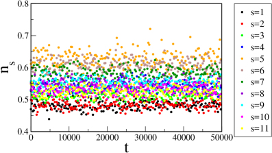
In Fig. 6 the long-time dynamics of the average occupation numbers

$$n_{s}(t)=\langle k_{0}|\hat{n}_{s}(t)|k_{0}\rangle$$

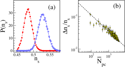
are shown for different $s$ values. Let us first concentrate on the statistical properties of this “classical signal”, $n_{s}(t)$. The distributions $P(n_{s})$, taken from the values in Fig. 6 are shown in Fig. 7(a) (for two values of $s$: $s=1$ and $s=M$). As one can see there is a very good agreement with a Gaussian fit. The width of these distributions (as given by the second moment of the fitted Gaussians $\Delta n_{s}^{2}$) weakly depends on the particular chosen $s$ value (see Fig. 7(a)) while the dependence on the initial state is stronger. To this end we compute the relative fluctuations $\Delta n_{s}/n_{s}$ choosing as initial states different unperturbed many-body basis states from the whole energy spectrum. In agreement what the results found for Fermi and Bose particles fi97 ; sm-BMI17 , we consider in Fig. 7(b) the relative fluctuations $\Delta n_{s}/n_{s}$ as a function of the number of principal components of the stationary wave-packet (after relaxation) for the correspondent initial states (essentially what is shown in Fig. 5(b).) As one can see there is a very good agreement with the dependence $1/\sqrt{\overline{N}_{pc}}$ which is a strong result in view of the requirement of statistical mechanics. Let us stress that the decrease of relative fluctuations occurs not with respect to the number $N$ of particles, but with the number of principal components contained in the stationary distribution $\overline{N}_{pc}$.

Concerning quantum fluctuations, they are defined by

$$\delta n_{s}^{2}(k_{0})=\overline{n_{s}^{2}}-(\overline{n_{s}})^{2}$$ (39)

for different initial states $\left|k_{0}\,\right\rangle$, and from them, the relative fluctuations $\delta n_{s}/\overline{n_{s}}$. In the canonical ensemble, for non-interacting bosons the following relation holds pathria ,

$$\frac{\delta n_{s}^{2}}{n_{s}^{2}}=1+\frac{1}{n_{s}}$$ (40)

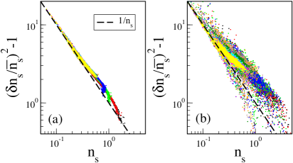
We have numerically checked this relation, see data in Fig.8(a) from which one can see a good correspondence to the above relation in the case when the eigenstates are strongly chaotic. In Fig.8(b), the same quantity has been plotted for a non-chaotic case. As one can see quantum fluctuations deviate strongly from the prediction given in Eq. (40). This result shows once more that even for a finite number of particles, provided a strong enough inter-particle interaction, conventional statistical mechanics works extremely well.

Figure 8: Relative quantum fluctuations $(\delta n_{s}/n_{s})^{2}-1$. Initial states $\left|k_{0}\,\right\rangle$ are basis states chosen in the whole energy spectrum. On $x$-axis the averaged values of $n_{s}$ are plotted. Dashed line is the theoretical prediction $1/n_{s}$. Different colors refer to different $s$ values. (a) $V=0.4$ case of strong quantum chaos, (b) $V=0.04$ case of non chaotic eigenstates for which Eq. (40) is not valid.

References

- (1) F. Borgonovi, F.M. Izrailev, L.F. Santos, Exponentially fast dynamics in the Fock space of chaotic many-body systems, arXiv:1802.08265 [cond-mat.stat-mech] (2018).
- (2) M. Rigol, V. Dunjko, and M. Olshanii, Thermalization and its mechanism for generic isolated quantum systems, Nature 452, (2008) 854; A. Polkovnikov, K. Sengupta, A. Silva, and M. Vengalattore, Colloquium: Nonequilibrium dynamics of closed interacting quantum systems, Rev. Mod. Phys. 83, (2011) 863; L. D’Alessio, Y. Kafri, A. Polkovnikov, and M. Rigol, From quantum chaos and eigenstate ther- malization to statistical mechanics and thermodynamics, Advances in Physics, 65, (2016) 239-362; D.J.Luitz and Y.B.Lev, Anomalous Thermalization in Ergodic Systems, Phys. Rev. Lett. 117, (2016) 170404.
- (3) L. F. Santos, F. Borgonovi, F. M. Izrailev Onset of chaos and relaxation in isolated systems of interacting spins: Energy shell approach, Phys. Rev. E 85, 036209 (2012); Chaos and statistical relaxation in quantum systems of interacting particles, Phys. Rev. Lett. 108, 094102 (2012); F. Borgonovi, F.M. Izrailev, L.F. Santos, V.G. Zelevinsky, Quantum chaos and thermalization in isolated systems of interacting particles, Physics Reports 626 (2016) 1.
- (4) M. Greiner, O. Mandel, T.W. Hansch, and I. Bloch, Collapse and revival of the matter wave field of a Bose–Einstein condensate, Nature 419, (2002) 51; S. Trotzky et. al., Probing the relaxation towards equilibrium in an isolated strongly correlated one-dimensional Bose gas, Nature Phys. 8, (2012) 325; M. Gring, et al., Relaxation and Prethermalization in an Isolated Quantum System, Science 337, (2012) 1318; A.M. Kaufman et al., Quantum thermalization through entanglement in an isolated many-body system, Science, 353 (2016), 794; R. Nandkishore and D.A. Huse, Many-Body Localization and Thermalization in Quantum Statistical Mechanics, Annual Review of Condensed Matter Physics 6 (2015) 15.
- (5) V.V. Flambaum, F.M. Izrailev, and G. Casati, Towards a Statistical Theory of Finite Fermi Systems and Compound States: Random Two-Body Interaction Approach, Phys. Rev. E 54, (1996) 2136; V.V. Flambaum, F.M. Izrailev, Distribution of Occupation Numbers in Finite Fermi-Systems and Role of Interaction in Chaos and Thermalization, Phys. Rev. E 55 (1997) R13; V.V. Flambaum and F.M. Izrailev, Statistical Theory of Finite Fermi-Systems Based on the Structure of Chaotic Eigenstates, Phys. Rev. E 56, (1997) 5144.
- (6) J.M. Deutsch, Quantum statistical mechanics in a closed system, Phys. Rev. A 43, (1991) 2046; J.M. Deutsch, Haibin Li and Auditya Sharma, Phys. Rev. E. 87, (2013) 042135; M. Srednicki, Phys. Rev. E 50, (1994) 888; J. Phys. A: Math. Gen. 29, (1996) L75.
- (7) V. Zelevinsky, B. A. Brown, N. Frazier, M. Horoi, The nuclear shell model as a testing ground for many-body quantum chaos, Phys. Rep. 276, 85 (1996).
- (8) F.Borgonovi, I.Guarneri, F.M.Izrailev, G.Casati, Chaos and Thermalization in a Dynamical Model of Two Interacting Particles, Phys. Lett. A 247, (1998) 140.
- (9) F. Borgonovi, G. Celardo, F.M. Izrailev, G. Casati, A semiquantal approach to finite systems of interacting particles, Phys. Rev. Lett. 88 (2002) 054101.
- (10) F. Borgonovi, F. Mattiotti and F. M. Izrailev, Temperature of a single chaotic eigenstate, Phys. Rev. E 95, 042135 (2017); F. Borgonovi and F. M. Izrailev, Localized thermal states, Conference Proceedings AIP Publishing, 1912, 020003 (2017).
- (11) G. F. Gribakin, A. A. Gribakina, and V. V. Flambaum, Quantum Chaos in Multicharged Ions and Statistical Approach to the Calculation of Electron–Ion Resonant Radiative Recombination, Aust. J. Phys. 52, 443 (1999).
- (12) S. Shenker and D. Stanford, Black holes and the butterfly effect, JHEP 1403 (2014) 067, [arXiv:1306.0622 [hep-th]]; J.M.Magan, Black hole, complexity and quantum chaos, arxiv:1805.05839 [hep-th].
- (13) J. Maldacena, S. H. Shenker, and D. Stanford, A bound on chaos, J. High Energy Phys. 2016:106, 1 (2016); D. Chowdhury, B. Swingle, Onset of many-body chaos in the O(N) model, arXiv:1703.02545 [cond-mat,str-el].
- (14) O. Bohigas and J. Flores, Two-body random Hamiltonian and level density, Phys. Lett. B 34, 261 (1971); Spacing and individual eigenvalue distributions of two-body random Hamiltonians, Phys. Lett. B 35, 383 (1971).
- (15) O. Bohigas and J. Flores, Two-body random Hamilto- nian and level density, Phys. Lett. B 34, 261 (1971); Spacing and individual eigenvalue distributions of two- body random Hamiltonians, Phys. Lett. B 35, 383 (1971); T. A. Brody, J. Flores, J. B. French, P. A. Mello, A. Pandey, S. S. M. Wong, Random-matrix physics: spectrum and strength fluctuations, Rev. Mod. Phys. 53, 385 (1981).
- (16) B. L. Altshuler, Y. Gefen, A. Kamenev, L. S. Levitov, Quasiparticle Lifetime in a Finite System: A Nonperturbative Approach, Phys. Rev. Lett. 78, 2803 (1997).
- (17) L. Benet and H. A. Weidenmüller, Review of the k-body embedded ensembles of Gaussian random matrices, J. Phys. A: Math. and Gen. 36, 3569 (2003); N. D. Chavda, V. K. B. Kota, V. Potbhare, Thermalization in one- plus two-body ensembles for dense interacting boson systems, Phys. Lett. A 376, 2972 (2012).
- (18) G. Casati, B. V Chirikov, I. Guarneri, F. M Izrailev, Band-random-matrix model for quantum localization in conservative systems, Phys. Rev. E 48, R1613 (1993), Quantum ergodicity and localization in conservative systems: the Wigner band random matrix model, Phys. Lett. A 223, 430 (1996).
- (19) A. Bohr, B. R. Mottelson, Nuclear Structure, (Benjamin, New York, 1969).
- (20) Supplemental Material.
- (21) K. Huang, Statistical Mechanics, John Wiley & Sons, (1987).
- (22) S. Sachdev and J. Ye, Gapless spin-fluid ground state in a random quantum Heisenberg magnet, Phys. Rev. Lett. 70, 3339 (1993); A. Kitaev, Talk given at the Fundamental Physics Prize Symposium, Nov. 10, 2014.
- (23) G.P. Berman, F. Borgonovi, F.M. Izrailev, A. Smerzi, Irregular Dynamics in a One-Dimensional Bose System, Phys. Rev. Lett. 92, (2004) 030404.
- (2) V. V. Flambaum and F. M. Izrailev, Statistical Theory of Finite Fermi-Systems Based on the Structure of Chaotic Eigenstates, Phys. Rev. E 56, 5144 (1997).
- (3) F. Borgonovi, F. Mattiotti and F. M. Izrailev, Temperature of a single chaotic eigenstate, Phys. Rev. E 95, 042135 (2017); F. Borgonovi and F. M. Izrailev, Localized thermal states, Conference Proceedings AIP Publishing, 1912, 020003 (2017).
- (4) R. K. Pathria, Paul D. Beale, Statistical Mechanics , Academic Press (2011).