Pattern Search Multidimensional Scaling

Abstract

We present a novel view of nonlinear manifold learning using derivative-free optimization techniques. Specifically, we propose an extension of the classical multi-dimensional scaling (MDS) method, where instead of performing gradient descent, we sample and evaluate possible “moves” in a sphere of fixed radius for each point in the embedded space. A fixed-point convergence guarantee can be shown by formulating the proposed algorithm as an instance of General Pattern Search (GPS) framework. Evaluation on both clean and noisy synthetic datasets shows that pattern search MDS can accurately infer the intrinsic geometry of manifolds embedded in high-dimensional spaces. Additionally, experiments on real data, even under noisy conditions, demonstrate that the proposed pattern search MDS yields state-of-the-art results.

1 INTRODUCTION

In the past decades, we have been witnessing a steady increase in the size of datasets generated and processed by computational systems. Such voluminous data comes from various sources, such as business sales records, the collected results of scientific experiments or real-time sensors used in the Internet of Things (IoT). The most popular way to represent such data is via a set of data points lying in a vector space. The construction of the vector space is often performed using a distance or similarity matrix that can be constructed manually using perceptual ratings or, more commonly, computed automatically using a set of features. In many of these applications high-dimensional data representations are assumed to lie in the vicinity of a low-dimensional, possibly non-linear manifold, embedded in the high-dimensional space. This is known as the manifold hypothesis [1]. Intuitively human cognition also performs similar mappings when performing everyday tasks, i.e., high-dimensional sensory input get embedded into low dimensional cognitive subspaces [2]; [3]; [4] for rapid and robust decision making, since only a small number of features are salient for each task. Given this assumption manifold learning aims to discover such hidden low-dimensional structure and to output a representation with much fewer “intrinsic variables”.

In this paper, we study the problem of manifold learning in non-metric topological spaces. The input to this problem is a matrix of (similarities or) dissimilarities of the dataset objects. “Objects” can be colors, faces, map coordinates, political persuasion scores, or any kind of real-world or synthetic stimuli. For each input dataset object, the output is a low-dimensional vector such that the pairwise Euclidean distances of the output vectors resemble the original dissimilarities. This problem is known as non-metric multidimensional scaling (MDS) or non-linear dimensionality reduction (NLDR) task. An abundance of embedding methods have been developed for dealing with this task as detailed in Section 2.

The majority of these algorithms reduce this problem to the optimization of a deterministic loss function $f$. Given this minimization objective, they usually employ gradient-based methods to find a global or a local optimum. In many situations, however, the loss function is non-differentiable or estimating its gradient may be computational expensive. Additionally, gradient-based algorithms usually yield a slow convergence; multiple iterations are needed in order to minimize the loss function.

Inspired by the recent progress in derivative-free optimization tools, we propose an iterative algorithm which treats the non-metric MDS task as a derivative-free optimization problem. The main contributions of the paper are as follows: 1) Using the General Pattern Search (GPS) formulation we are able to provide theoretical convergence guarantees for the proposed non-metric MDS algorithm. 2) A set of heuristics are proposed that significantly improve the performance of the proposed algorithm in terms of computational efficiency, convergence rate and solution accuracy. 3) The proposed algorithm is evaluated on a variety of tasks including manifold unfolding, word embeddings and optical digit recognition, showing consistent performance and good convergence properties. We also compare performance with state-of-the-art MDS algorithms for the aforementioned tasks for clean and noisy datasets. An optimized implementation of pattern search MDS and the experimental code is made available as open source to the research community.

The remainder of the paper is organized as follows: We begin with an overview of the related work in Section 2. Then in Section 3, we review several optimization problems that are related to the manifold learning task and we present the GPS framework. Then in Section 4, we present in detail the proposed derivative-free algorithm, a sketch of the reduction of the algorithm to the GPS formulation and the associated proof of fixed-point convergence guarantees. Finally in Section 5, the proposed algorithm is compared and contrasted with other dimensionality reduction methods in a variety of tasks with or without the presence of noise. We conclude and present future directions for research in Sections 6 and 7, respectively.

2 RELATED WORK

Loosely speaking, a manifold is a topological space that locally resembles a Euclidean space. The purpose of Multidimensional Scaling (MDS) is to infer data representations on a low-dimensional manifold while simultaneously preserving the distances of the high-dimensional data points. When data lies on or close to a linear subspace, low-dimensional representations of data can be obtained using linear dimensionality reduction techniques like Principle Components Analysis (PCA) [5] and classical MDS.

In real data applications, such a linearity assumption may be too strong and can lead to meaningless results. Thus a significant effort has been made by the machine learning community to apply manifold learning in non-linear domains. Representative manifold learning algorithms include Isometric Feature Mapping (ISOMAP) [6, 7, 8, 9, 10], Landmark ISOMAP [11, 12],Locally Linear Embedding (LLE) [13, 14, 15, 16, 17], Modified LLE [18] Hessian LLE [19, 20], Semidefinite Embedding [21], [22], [23], [24], Laplacian Eigenmaps (LE) [25, 13, 26], Local Tangent Space Alignment (LTSA) [27],etc. ISOMAP uses a geodesic distance to measure the geometric information within a manifold. LLE assumes that a manifold can be approximated in a Euclidean space and the reconstruction coefficients of neighbors can be preserved in the low-dimensional space. LE uses an undirected weighted graph to preserve local neighbor relationships. Hessian LLE obtains low-dimensional representations through applying eigenanalysis on a Hessian coefficient matrix. LTSA utilizes local tangent information to represent the manifold geometry and extends this to global coordinates. Finally, SDE attempts to maximize the distance between points that don’t belong in a local neighborhood. Also, a common nonlinear method for dimensionality reduction is the kernel extension of PCA [28].

A wide class of derivative-free algorithms for nonlinear optimization has been studied and analyzed in [29] and [30]. GPS methods consist a subset of the aforementioned algorithms which do not require the explicit computation of the gradient in each iteration-step. Some GPS algorithms are: the original Hooke and Jeeves pattern search algorithm [31], the evolutionary operation by utilizing factorial design [32] and the multi-directional search algorithm [33], [34]. In [35], a unified theoretical formulation of GPS algorithms under a common notation model has been presented as well as an extensive analysis of their global convergence properties. Local convergence properties have been studied later by [36]. Notably, the theoretical framework as well as the convergence properties of GPS methods have been extended in cases with linear constrains [37], boundary constrains [38] and general Lagrangian formulation [39].

3 PRELIMINARIES

3.1 Notation

We denote real, integer and natural numbers as $\mathbb{R}$, $\mathbb{Z}$, $\mathbb{N}$, respectively. Scalars are represented by no-boldface letters, vectors appear in boldface lowercase letters and matrices are indicated by boldface uppercase letters. All vectors are assumed to be column vectors unless they are explicitly defined as row vectors. For a vector $\mathbf{z}\in\mathbb{R}^{n}$, $\|\mathbf{z}\|_{1}=\sum_{i=1}^{n}|z_{i}|$ is its ${\ell}_{1}$ norm and $\|\mathbf{z}\|_{2}=\sqrt[]{\sum_{i=1}^{n}z_{i}^{2}}$ is its ${\ell}_{2}$ norm, where $z_{i}$ is the ith element of $\mathbf{z}$. By $\mathbf{A}\in\mathbb{R}^{n\times m}$ we denote a real-valued matrix with n rows and m columns. Additionally, the $j$th column of the matrix $\mathbf{A}$ and its entry at $i$th row and $j$th column are referenced as $\mathbf{a}_{j}$ and $a_{ij}$, respectively. The trace of the matrix $\mathbf{A}$ appears as $tr(\mathbf{A})$ and its Frobenius norm as $||\mathbf{A}||_{F}=\sqrt[]{\sum_{i=1}^{n}\sum_{j=1}^{m}a_{ij}^{2}}$. The square identity matrix with $n$ rows is denoted as $\mathbf{I}_{n}\in\mathbb{R}^{n\times n}$. For the matrices $\mathbf{A}\in\mathbb{R}^{n\times m}$ and $\mathbf{B}\in\mathbb{R}^{n\times m}$ we indicate their Hadamard product as $\mathbf{A}\odot\mathbf{B}$. The $n$-ary Cartesian product over $n$ sets $S_{1},...,S_{n}$ is denoted by $\{(s_{1},...,s_{n}):s_{i}\in S_{i}.\enskip 1\leq i\leq n\}$ Finally, $\mathbf{X}^{(k)}$ refers to the estimate of a variable $\mathbf{X}$ at the $k$th iteration of an algorithm.

3.2 Classical MDS

Classical MDS was first introduced by [40] and can be formalized as follows. Given the matrix $\mathbf{\Delta}$ consisting of pairwise distances or dissimilarities $\{\delta_{ij}\}_{1\leq i,j\leq N}$ between $N$ points in a high dimensional space, the solution to Classical MDS is given by a set of points $\{\mathbf{x}_{i}\}_{i=1}^{N}$ which lie on the manifold $\mathcal{M}\in\mathbb{R}^{L}$ and their pairwise distances are able to preserve the given dissimilarities $\{\delta_{ij}\}_{1\leq i,j\leq N}$ as faithfully as possible. Each point $\mathbf{x}_{i}\in\mathbb{R}^{L},\enskip 1\leq i\leq N$ corresponds to a column of the matrix $\mathbf{X}^{T}\in\mathbb{R}^{L\times N}$. The embedding dimension $L$ is selected as small as possible in order to obtain the maximum dimensionality reduction but also to be able to approximate the given dissimilarities $\delta_{ij}$ by the Euclidean distances $d_{ij}(\mathbf{X})=||\mathbf{x}_{i}-\mathbf{x}_{j}||_{2}=\sqrt{\sum_{k=1}^{L}(x_{ik}-x_{jk})^{2}}$ in the embedded space $\mathbb{R}^{L}$.

The proposed algorithm uses a centering matrix $\mathbf{H}=\mathbf{I}_{N}-\frac{1}{N}\mathbf{1}_{N}^{T}\mathbf{1}_{N}$ in order to subtract the mean of the columns and the rows for each element. Where $\mathbf{1}_{N}=[1,1,...,1]$ a vector of ones in $\mathbb{R}^{N}$ space. By applying the double centering to the Hadamard product of the given dissimilarities, the Gram matrix $\mathbf{B}$ is constructed as follows:

$$\mathbf{B}=-\frac{1}{2}\mathbf{H}^{T}(\mathbf{\Delta}\odot\mathbf{\Delta})\mathbf{H}$$ (1)

It can be shown (Ch. 12 [41]) that classical MDS minimizes the Strain algebraic criterion in Eq. 2 below:

$$||\mathbf{X}\mathbf{X}^{T}-\mathbf{B}||_{F}^{2}$$ (2)

The eigendecomposition of the symmetric matrix $\mathbf{B}$ gives us $\mathbf{B}=\mathbf{V}\mathbf{\Lambda}\mathbf{V}^{T}$ and thus the new set of points consisting the embedding in $\mathbb{R}^{L}$ are given by the first $L$ positive eigenvalues of $\mathbf{\Lambda}$, namely $\mathbf{X}=\mathbf{V}_{L}$. This solution provides the same result as Principal Component Analysis (PCA) applied on the vector in the high dimensional space [42]. Classic MDS was originally proposed for dissimilarity matrices $\mathbf{\Delta}$ which can be embedded with good approximation accuracy in a low-dimensional Euclidean space. However, matrices which correspond to embeddings in Euclidean sub-spaces [43], Poincare disks [44] and constant-curvature Riemannian spaces [45] have also been studied.

3.3 Metric MDS

Metric MDS describes a superset of optimization problems containing classical MDS. Shepard has introduced heuristic methods to enable transformations of the given dissimilarities $\delta_{ij}$ [46], [47] but did not provide any loss function in order to model them [48]. Kruskal in [49] and [50] formalized the metric MDS as a least squares optimization problem of minimizing the non-convex Stress-1 function defined in Eq. 3 shown next:

$$\sigma_{1}(\mathbf{X},\hat{\mathbf{D}})=\sqrt[]{\frac{\sum_{i=1}^{N}\sum_{j=1}^{N}(\hat{d_{ij}}-d_{ij}(\mathbf{X}))}{\sum_{i=1}^{N}\sum_{j=1}^{N}d_{ij}^{2}(\mathbf{X})}}$$ (3)

where matrix $\hat{\mathbf{D}}$ with elements $\hat{d_{ij}}$ represents all the pairs of the transformed dissimilarities $\delta_{ij}$ that are used to fit the embedded distance pairs $d_{ij}(\mathbf{X})$.

In essence, $\hat{d_{ij}}=\mathcal{F}(\delta_{ij})$ where $\mathcal{F}$ is usually an affine transformation $\hat{d_{ij}}=\alpha+\beta\delta_{ij}$ for unknown $\alpha$ and $\beta$. Kruskal proposed an iterative gradient-based algorithm for the minimization of $\sigma_{1}$ since the solution cannot be expressed in closed form. Assuming that $\hat{d_{ij}=\delta_{ij}}$ the algorithm iteratively tries to find the coordinates of points $\mathbf{X}$ which are lying in the low embedding space $\mathbb{R}^{L}$. Trivial solutions ($\mathbf{X}=\mathbf{0}$ and $\hat{\mathbf{D}}=\mathbf{0}$) are avoided by the denominator term in Eq. 3.

A weighted MDS raw Stress function is defined as:

$$\sigma_{raw}^{2}(\mathbf{X},\hat{\mathbf{D}})=\sum_{i=1}^{N}\sum_{j=1}^{N}w_{ij}(\hat{d_{ij}}-d_{ij}(\mathbf{X}))^{2}$$ (4)

where the weights $w_{ij}$ are restricted to be non-negative; for missing data the weights are set equal to zero. By setting $w_{ij}=1,\forall 1\leq i,j\leq N$ one can model an equal contribution to the Metric-MDS solution for all the elements.

3.4 SMACOF

SMACOF which stands for Scaling by Majorizing a Complex Function is a state-of-the-art algorithm for solving metric MDS and was introduced by [52]. By setting $\hat{d_{ij}}=\delta_{ij}$ in raw stress function defined in Eq. 4, SMACOF minimizes the resulting stress function $\sigma_{raw}^{2}(\mathbf{X})$.

$$\sigma^{2}(\mathbf{X})=\sum_{i=1}^{N}\sum_{j=1}^{N}w_{ij}(\delta_{ij}^{2}-2\delta_{ij}d_{ij}(\mathbf{X})+d_{ij}^{2}(\mathbf{X}))$$ (5)

The algorithm proceeds iteratively and decreases stress monotonically up to a fixed point by optimizing a convex function which serves as an upper bound for the non-convex stress function in Eq. 5. An extensive description of SMACOF can be found in [41] while its convergence for a Euclidean embedded space $\mathbb{R}^{L}$ has been proven by [53].

Let matrices $\mathbf{U}$ and $\mathbf{R(\mathbf{X})}$ be defined element-wise as follows:

$$u_{ij}=\left\{\begin{array}[]{ll}-w_{ij}&i\neq j\\ \sum_{k\neq i}w_{ik}&i=j\end{array}\right.$$ (6)

$$r_{ij}=\left\{\begin{array}[]{ll}-w_{ij}\delta_{ij}d_{ij}^{-1}(\mathbf{X})&i\neq j,d_{ij}(\mathbf{X})\neq 0\\ 0&i\neq j,d_{ij}(\mathbf{X})=0\\ \sum_{k\neq i}r_{ik}&i=j\end{array}\right.$$ (7)

The stress function in Eq. 5 is converted to the following quadratic form:

$$\sigma^{2}(\mathbf{X})=\sum_{i=1}^{N}\sum_{j=1}^{N}w_{ij}\delta_{ij}^{2}-2tr(\mathbf{X}^{T}\mathbf{R}(\mathbf{X})\mathbf{X})+tr(\mathbf{X}^{T}\mathbf{U}\mathbf{X})$$ (8)

The quadratic can be minimized iteratively as follows:

$$\begin{split}T(\mathbf{X},\hat{\mathbf{X}}^{(k)})&=c-2tr(\mathbf{X}^{T}\mathbf{R}(\hat{\mathbf{X}}^{(k)})\hat{\mathbf{X}}^{(k)})+tr(\mathbf{X}^{T}\mathbf{U}\mathbf{X})\\ &c=\sum_{i=1}^{N}\sum_{j=1}^{N}w_{ij}\delta_{ij}^{2}=const.\end{split}$$ (9)

$$\hat{\mathbf{X}}^{(k+1)}=\underset{\mathbf{X}}{\operatorname{argmin}}\;{T(\mathbf{X},\hat{\mathbf{X}}^{(k)})}=\mathbf{U}^{\dagger}\mathbf{R}(\hat{\mathbf{X}}^{(k)})\hat{\mathbf{X}}^{(k)}$$ (10)

where $\hat{\mathbf{X}}^{(k)}$ is the estimate of matrix $\mathbf{X}$ at the $k$th iteration and $\mathbf{U}^{\dagger}$ is Moore-Penrose pseudoinverse of $\mathbf{U}$. At iteration $k$ the convex majorizing convex function touches the surface of $\sigma$ at the point $\hat{\mathbf{X}}^{(k)}$. By minimizing this simple quadratic function in Eq. 9 we find the next update which serves as a starting point for the next iteration $k+1$. The solution to the minimization problem is shown in Eq. 10. The algorithm stops when the new update yields a decrease $\sigma^{2}(\hat{\mathbf{X}}^{(k+1)})-\sigma^{2}(\hat{\mathbf{X}}^{(k)})$ that is smaller than a threshold value.

3.5 GPS formulation

The unconstrained problem of minimizing a continuously differentiable function $f:\mathbb{R}^{n}\rightarrow\mathbb{R}$ is formally described as

$$\mathbf{x}^{*}=\underset{\mathbf{x}\in\mathbb{R}^{n}}{\operatorname{argmin}}\;f(\mathbf{x})$$ (11)

Next we present a short description of iterative GPS minimization of Eq. 11 based on [35, 36]. First we have to define the following components:

• A basis matrix that could be any nonsingular matrix $\mathbf{B}\in\mathbb{R}^{n\times n}$.

• A matrix $\mathbf{C}^{(k)}$ for generating all the possible moves for the $k$th iteration of the minimization algorithm

  $$\mathbf{C}^{(k)}=[\mathbf{M}^{(k)}\enskip-\mathbf{M}^{(k)}\enskip\mathbf{L}^{(k)}]=[\mathbf{\Gamma}^{(k)}\enskip\mathbf{L}^{(k)}]$$ (12)

  where the columns of $\mathbf{M}^{(k)}\in\mathbb{Z}^{n\times n}$ form a positive span of $\mathbb{R}^{n}$ and $\mathbf{L}^{(k)}$ contains at least the zero column of the search space $\mathbb{R}^{n}$.

• A pattern matrix $\mathbf{P}^{(k)}$ defined as

  $$\mathbf{P}^{(k)}=\mathbf{B}\mathbf{C}^{(k)}=[\mathbf{B}\mathbf{M}^{(k)}\enskip-\mathbf{B}\mathbf{M}^{(k)}\enskip\mathbf{B}\mathbf{L}^{(k)}]$$ (13)

  where the submatrix $\mathbf{B}\mathbf{M}^{(k)}$ forms a basis of $\mathbb{R}^{n}$.

In each iteration $k$, we define a set of steps $\{\mathbf{s}_{i}^{(k)}\}_{i=1}^{m}$ generated by the pattern matrix $\mathbf{P}^{(k)}$ as shown next:

$$\mathbf{s}_{i}^{(k)}=\Delta^{(k)}\mathbf{p}_{i}^{(k)},\enskip\mathbf{P}^{(k)}=[\mathbf{p}_{1}^{(k)},...,\mathbf{p}_{m}^{(k)}]\in\mathbb{R}^{n\times m}$$ (14)

where $\mathbf{p}_{i}^{(k)}$ is the $i$th column of $\mathbf{P}^{(k)}$ and defines the direction of the new step, while $\Delta^{(k)}$ configures the length towards this direction. If the pattern matrix $\mathbf{P}^{(k)}$ contains $m$ columns, then $m\geq n+1$ in order to positively span the search space $\mathbb{R}^{n}$. Thus, a new trial point of GPS algorithm towards this step would be $\mathbf{x}_{i}^{(k+1)}=\mathbf{x}^{(k)}+\mathbf{s}_{i}^{(k)}$ where we evaluate the value of the function $f$ to minimize. The success of a new trial point is decided based on the condition that it takes a step towards further minimizing the function $f$, i.e., $f(\mathbf{x}^{(k)}+\mathbf{s}_{i}^{(k)})>f(\mathbf{x}_{i}^{(k+1)})$. The steps of a GPS method are presented in Alg. 1.

Algorithm 1 General Pattern Search (GPS)

1:procedure GPS_SOLVER($\mathbf{x}^{(0)}$, $\Delta^{(0)}$, $\mathbf{C}^{(0)}$, $\mathbf{B}$)

2:     $k=-1$

3:     do

4:         $k=k+1$

5:         $\mathbf{s}^{(k)}=$ EXPLORE_MOVES($\mathbf{B}\mathbf{C}^{(k)}$, $\mathbf{x}^{(k)}$, $\Delta^{(k)}$)

6:         $\rho^{(k)}=f(\mathbf{x}^{(k)}+\mathbf{s}^{(k)})-f(\mathbf{x}^{(k)})$

7:         if $\rho^{(k)}<0$ then

8:              $\mathbf{x}^{(k+1)}=\mathbf{x}^{(k)}+\mathbf{s}^{(k)}$ $\triangleright$ Successful iteration

9:         else

10:              $\mathbf{x}^{(k+1)}=\mathbf{x}^{(k)}$ $\triangleright$ Unsuccessful iteration          

11:         $\Delta^{(k+1)},\mathbf{C}^{(k+1)}=$ UPDATE($\mathbf{C}^{(k)}$, $\Delta^{(k)}$, $\rho^{(k)}$)

12:     while convergence criterion == False

To initialize the algorithm we select a point $\mathbf{x}^{(0)}\in\mathbb{R}^{n}$ and a positive step length parameter $\Delta^{(0)}>0$. In each iteration $k$, we explore a set of moves defined by the $\texttt{EXPLORE\_MOVES}()$ subroutine at line 5 of the algorithm. Pattern search methods described using a GPS formalism mainly differ on the heuristics used for the selection of exploratory moves. If a new exploratory point lowers the value of the function $f$, iteration $k$ is successful and the starting point of the next iteration is updated $\mathbf{x}^{(k+1)}=\mathbf{x}^{(k)}+\mathbf{s}^{(k)}$ as shown in line 8, else there is no update. The step length parameter $\Delta^{(k)}$ is modified by the $\texttt{UPDATE}()$ subroutine in line 11. For successful iterations, i.e., $\rho^{(k)}<0$, the step length is forced to increase in a determistic way as follows:

$$\begin{split}&\Delta^{(k+1)}=\lambda^{(k)}\Delta^{(k)},\enskip\lambda^{(k)}\in\Lambda=\{\tau^{w_{1}},...,\tau^{w_{|\Lambda|}}\}\\ &\tau>1,\enskip\{w_{1},...,w_{|\Lambda|}\}\subset\mathbb{N},\enskip|\Lambda|<+\infty\end{split}$$ (15)

where $\tau$ and $w_{i}$ are predefined constants that are used for the $i$th successive successful iteration. For unsuccessful iterations the step length parameter is decreased, i.e., $\Delta^{(k+1)}\leq\Delta^{(k)}$ as follows:

$$\Delta^{(k+1)}=\theta\Delta^{(k)},\enskip\theta=\tau^{w_{0}},\enskip\tau>1,\enskip w_{0}<0,$$ (16)

where $\tau$ and the negative integer $w_{0}$ determine the fixed ratio of step reduction. Note that the generating matrix $\mathbf{C}^{(k+1)}$ could be also updated for unsuccessful/successful iterations in order to contain more/less search directions, respectively.

3.6 GPS Convergence

GPS methods under the aforementioned defined framework have some important convergence properties shown in [35, 36, 38, 39, 37] and summarized here. For any GPS method which satisfies the specifications of Hyp. 1 on the exploratory moves one may be able to show convergence for Alg. 1.

Hypothesis 1 (Weak Hyp. on Exploratory Moves):

The subroutine
$\texttt{EXPLORE\_MOVES}()$ as defined in Alg. 1, line 5 guarantees the following:

• The exploratory step direction for iteration $k$ is selected from the columns of the pattern matrix $\mathbf{P}^{(k)}$ as defined in Eq. 14 and the exploratory step length is ${\Delta^{(k)}}$ as defined in Eqs. 15, 16.

• If among the exploratory moves $\mathbf{a}^{(k)}$ at iteration $k$ selected from the columns of the matrix $\Delta^{(k)}\mathbf{B}[\mathbf{M}^{(k)}-\mathbf{M}^{(k)}]$ exist at least one move that leads to success, i.e., $f(\mathbf{x}^{(k)}+\mathbf{a})<f(\mathbf{x}^{(k)})$, then the $\texttt{EXPLORE\_MOVES}()$ subroutine will return a move $\mathbf{s}^{(k)}$ such that $f(\mathbf{x}^{(k)}+\mathbf{s}^{(k)})<f(\mathbf{x}^{(k)})$.

Hyp. 1 enforces some mild constraints on the configuration of the exploratory moves produced by Alg. 1, line 5. Essentially, the suggested step $\mathbf{s}^{(k)}$ is derived from the pattern matrix $\mathbf{P}^{(k)}$, while the algorithm needs to provide a simple decrease for the objective function $f$. Specifically, the only way to accept an unsuccessful iteration would be if none of the steps from the columns of the matrix $\Delta^{(k)}\mathbf{B}[\mathbf{M}^{(k)}-\mathbf{M}^{(k)}]$ lead to a decrease of the objective function $f$. Based on this hypothesis one can formulate Thm. 1 as follows:

Theorem 1:

Let $L(\mathbf{x}^{*})=\{\mathbf{x}:f(\mathbf{x})\leq f(\mathbf{x}^{*})\}$ be closed and bounded and $f$ continuously differentiable on a neighborhood of $L(\mathbf{x}^{*})$, namely on the union of the open balls $\underset{{\mathbf{a}\in L(\mathbf{x}^{*})}}{\bigcup}B(\mathbf{a},\eta)$ where $\eta>0$. If a GPS method is formulated as described in Section 3.5 and Hyp. 1 holds then for the sequence of iterations $\{\mathbf{x}^{(k)}\}$ produced by Alg. 1

$$\underset{k\rightarrow+\infty}{\lim}\inf\;||\nabla f(\mathbf{x}^{(k)})||=0$$

Proof 1:

See [35].

As shown in [54] one can construct a continuously differentiable objective function and a GPS method with infinite many limit points with non-zero gradients and thus even Thm. 1 holds, the convergence of $||\nabla f(x_{k})||$ is not assured. However, the convergence properties of GPS methods can be further strengthened if additional criteria are met. Specifically, a stronger hypothesis on exploratory moves Hyp. 2 regulates the measure of decrease of the objective function for each step produced by the GPS method, as follows:

Hypothesis 2 (Strong Hyp. on Exploratory Moves):

The subroutine $\texttt{EXPLORE\_MOVES}()$ as defined in Alg. 1, line 5 guarantees the following:

• The exploratory step direction for iteration $k$ is selected from the columns of the pattern matrix $\mathbf{P}^{(k)}$ as defined in Eq. 14 and the exploratory step length is ${\Delta^{(k)}}$ as defined in Eqs. 15, 16.

• If among the exploratory moves $\mathbf{a}^{(k)}$ at iteration $k$ selected from the columns of the matrix $\Delta^{(k)}\mathbf{B}[\mathbf{M}^{(k)}-\mathbf{M}^{(k)}]$ exists at least one move that leads to success, i.e., $f(\mathbf{x}^{(k)}+\mathbf{a})<f(\mathbf{x}^{(k)})$, then the $\texttt{EXPLORE\_MOVES}()$ subroutine will return a move $\mathbf{s}^{(k)}$ such that:
  $f(\mathbf{x}^{(k)}+\mathbf{s}^{(k)})\leq\underset{\mathbf{a}^{(k)}}{\operatorname{min}}\;f(\mathbf{x}^{(k)}+\mathbf{a}^{(k)})$.

Hyp. 2 enforces the additional strong constraint on the configuration of the exploratory moves, namely that the subroutine $\texttt{EXPLORE\_MOVES}()$ will do no worse than produce the best exploratory move from the columns of the matrix $\Delta^{(k)}\mathbf{B}[\mathbf{M}^{(k)}-\mathbf{M}^{(k)}]$. Based on this hypothesis and by adding requirements restricting the exploration step direction and length for the GPS method, one can formulate Thm. 2 which is also presented here without proof.

Theorem 2:

Let $L(\mathbf{x}^{*})=\{\mathbf{x}:f(\mathbf{x})\leq f(\mathbf{x}^{*})\}$ be closed and bounded and $f$ continuously differentiable on a neighborhood of $L(\mathbf{x}^{*})$, namely on the union of the open balls $\underset{{\mathbf{a}\in L(\mathbf{x}^{*})}}{\bigcup}B(\mathbf{a},\eta)$ where $\eta>0$. If a GPS method is formulated as described in Section 3.5, $\underset{k\rightarrow+\infty}{\lim}\Delta^{(k)}=0$, the columns of the generating matrices $\mathbf{C}^{(k)}$ are bounded by norm and Hyp. 2 holds then for the sequence of iterations $\{\mathbf{x}^{(k)}\}$ produced by Alg. 1

$$\underset{k\rightarrow+\infty}{\lim}\;||\nabla f(\mathbf{x}^{(k)})||=0$$

Proof 2:

See [35].

The additional requirements specify that: 1) the generating matrix $\mathbf{C}^{(k)}$ should be norm bounded in order to produce trial steps from Eq. 14 that are bounded by the step length parameter $\Delta^{(k)}$ and 2) $\underset{k\rightarrow+\infty}{\lim}\Delta^{(k)}=0$ that can be easily met by selecting $\Lambda=\{1\}$ in Eq. 16; this also guarantees a non increasing sequence of $\Delta^{(k)}$ steps [35]. Although these criteria provide much stronger convergence properties, we are faced with a trade off between the theoretical proof of convergence and the efficiency of heuristics in finding a local optimum.

Both theorems 1 and 2 provide a first order optimality condition if their specifications hold. Although the latter theorem premises much stronger convergence results, step-length control parameter $\Delta^{(k)}$, provides a reliable asymptotic measure of first-order stationarity when it is reduced after unsuccessful iterations [36].

4 Pattern Search MDS

4.1 Core algorithm

The key idea behind the proposed algorithm is to treat MDS as a derivative-free problem, using a variant of general pattern search optimization to minimize a loss function. The input to pattern search MDS is a $N\times N$ target dissimilarity matrix $\mathbf{T}$ and the target dimension $L$ of the embedding space. An overview of the algorithm shown in Alg. 2 is presented next.

The initialization process of the algorithm consists of: 1) random sampling of $N$ points in the embedded space and construction of the matrix $\mathbf{X}^{(0)}=[\mathbf{x}_{1}^{(0)},\mathbf{x}_{2}^{(0)},...,\mathbf{x}_{N}^{(0)}]\in\mathbb{R}^{N\times L}$, 2) computing the embedded space dissimilarity matrix $\mathbf{D}^{(0)}$, where the element $d_{ij}^{(0)}$ is the Euclidean distance between vectors $\mathbf{x}_{i}^{(0)}$ and $\mathbf{x}_{j}^{(0)}$ of $\mathbf{X}^{(0)}$, and 3) computing the initial approximation error $e^{(0)}=f(\mathbf{T},\mathbf{D}^{(0)})$, where $e$ is the element-wise mean squared error (MSE) between the two matrices. The functional $f$ that we attempt to minimize is the normalized square of the Frobenius norm of the matrix $\mathbf{T}-\mathbf{D}$, i.e., $f(\mathbf{T},\mathbf{D})=(1/N^{2})||\mathbf{T}-\mathbf{D}||_{F}^{2}$. Equivalently one may express $f$ element-wise as follows:

$$f(\mathbf{T},\mathbf{D})=\frac{1}{N^{2}}\sum_{i=1}^{N}\sum_{j=1}^{N}(t_{ij}-d_{ij})^{2},\enskip\;\mbox{where}\;\mathbf{T},\mathbf{D}\in\mathbb{R}^{N\times N}$$ (17)

Algorithm 2 Proposed MDS

1:procedure MDS($\mathbf{T}$, $L$, $r^{(0)}$)

2:     $k$ $\leftarrow$ $0$ $\triangleright$ k is the number of epochs

3:     $\mathbf{X}^{(k)}$ $\leftarrow$ UNIFORM($N\times L$)

4:     $\mathbf{D}^{(k)}$ $\leftarrow$ DISTANCE_MATRIX($\mathbf{X}^{(k)}$)

5:     $e^{(k)}$ $\leftarrow$ $f(\mathbf{T},\mathbf{D}^{(k)})$

6:     $e^{(k-1)}$ $\leftarrow$ $+\infty$

7:     $r^{(k)}$ $\leftarrow$ $r^{(0)}$

8:     while $r^{(k)}>\delta$ do

9:         if $e^{(k-1)}-e^{(k)}\leq\epsilon\cdot e^{(k)}$ then

10:              $r^{(k)}$ $\leftarrow$ $\frac{r^{(k)}}{2}$          

11:         $\mathbf{S}$ $\leftarrow$ SEARCH_DIRECTIONS($r^{(k)}$, $L$)

12:         for all $x\in\mathbf{X}^{(k)}$ do

13:              $\mathbf{X^{*}},e^{*}$ $\leftarrow$ OPTIMAL_MOVE($\mathbf{X}^{(k)}$,$x$,$\mathbf{S}$,$e^{(k)}$)

14:              $e^{(k-1)}\leftarrow e^{(k)}$

15:              $e^{(k)}$ $\leftarrow$ $e^{*}$

16:              $\mathbf{X}^{(k)}$ $\leftarrow$ $\mathbf{X^{*}}$          

17:         $k=k+1$      

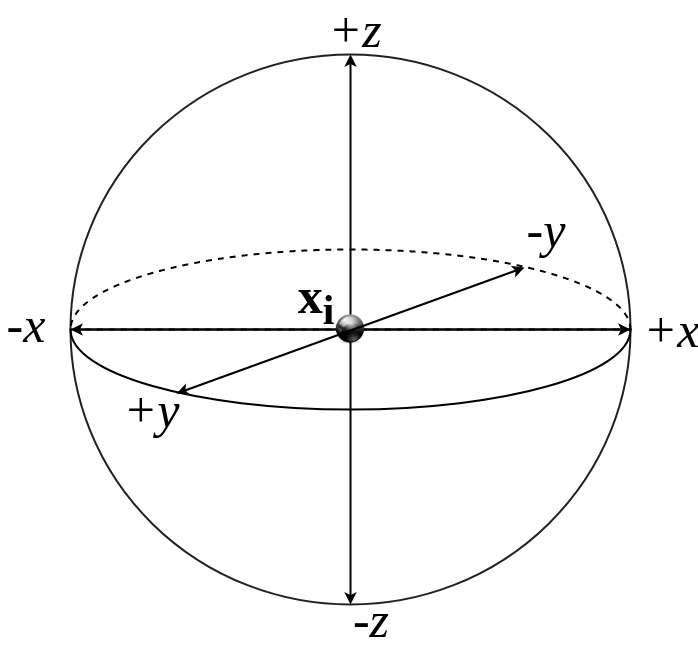
Following the initialization steps, in each epoch (iteration), we consider the surface of a hypersphere of radius $r$ around each point $\mathbf{x}^{(k)}_{i}$. The possible search directions lie on the surface of a hypersphere along the orthogonal basis of the space, e.g., in the case of $3$-dimensional space along the directions $\pm x,\pm y,\pm z$ on the sphere shown in Fig. 1. This creates the search directions matrix $S$ and is summarized in Alg. 3

Figure 1: Sphere of radius $r$ around point $\mathbf{x^{(k)}_{i}}$ and possible search directions

Algorithm 3 Define search directions

1:function SEARCH_DIRECTIONS($r$, $L$)

2:     $\mathbf{S^{+}}$ $\leftarrow$ $r\cdot\mathbf{I}_{L}$

3:     $\mathbf{S^{-}}$ $\leftarrow$ $-r\cdot\mathbf{I}_{L}$

4:     $\mathbf{S}$ $\leftarrow$ $[\frac{\mathbf{S^{+}}}{\mathbf{S^{-}}}]$

5:     return $S$

Each point is moved greedily along the dimension that produces the minimum error. At this stage we only consider moves that yield a monotonic decrease in the error function. Alg. 4 finds the optimal move that minimizes $e^{(k)}=f(\mathbf{T},\mathbf{D}^{(k)})$ for each new point $\tilde{x}$ and moves $\mathbf{X}$ in that direction. Note that when writing $s\in\mathbf{S}$, the matrix $\mathbf{S}$ is considered to be a set of row vectors.

Algorithm 4 Find optimal move for a point

1:function OPTIMAL_MOVE($\mathbf{X}^{(k)}$, $x$, $S$, $e$)

2:     $e^{*}\leftarrow e$

3:     for all $s\in\mathbf{S}$ do

4:         $\tilde{x}$ $\leftarrow$ $x+s$

5:         $\mathbf{\tilde{X}}$ $\leftarrow$ UPDATE_POINT($\mathbf{X}^{(k)}$, $x$, $\tilde{x}$) $\triangleright$ Update $x$ point of $\mathbf{X}^{(k)}$ with $\tilde{x}$

6:         $\mathbf{D}$ $\leftarrow$ DISTANCE_MATRIX($\mathbf{\tilde{X}}$)

7:         $\tilde{e}$ $\leftarrow$ f($\mathbf{T}$, $\mathbf{D}$)

8:         if $\tilde{e}<e^{*}$ then

9:              $e^{*}$ $\leftarrow$ $\tilde{e}$

10:              $\mathbf{X}^{*}$ $\leftarrow$ $\mathbf{\tilde{X}}$               

11:     return $X^{*},e^{*}$

The resulting error $e^{*}$ is computed after performing the optimal move for each point in $\mathbf{X}^{(k)}$. If the error decrease hits a plateau, we halve the search radius and proceed to the next epoch. This is expressed as $e^{(k)}-e^{*}<\epsilon\cdot e^{(k)}$, where $\epsilon$ is a small positive constant, namely the error decrease becomes very small in relation to $e^{(k)}$. The process stops when the search radius $r$ becomes very small, namely $r<\delta$, where $\delta$ is a small constant, as shown in Alg. 2.

4.2 Optimizations and algorithm complexity

Next, a set of algorithmic optimizations are presented that can improve the execution time and the solution quality of Alg. 2. We also present ways to improve the execution time by searching for an approximate solution, as well as, discuss ways to utilize parallel computation for parts of the algorithm.

4.2.1 Allow for “bad” moves

In Section 4.1 we restrict the accepted moves so that the error decreases monotonically. This is a reasonable restriction that also provides us with theoretical guarantees of convergence. Nonetheless in our experimental setting, we observed that if we relax this restriction and allow each point to always make the optimal move, regardless if the error (temporarily) increases the algorithm converges faster to better solutions. The idea of allowing greedy algorithms to make some “bad” moves in hope to get over local minima can be found in other optimization algorithms, simulated annealing [55] being the most popular. To implement this one can modify line 13 in Alg. 2 to:

$\mathbf{X^{*}},e^{*}$ $\leftarrow$ OPTIMAL_MOVE($\mathbf{X}^{(k)}$, $x$, $S$, $+\infty$)

4.2.2 Online computation of dissimilarity matrix

In line 6 of Alg. 4 we observe that we recompute the dissimilarity matrix for each move. This can be avoided because each move modifies only one point $\mathbf{x}^{(k)}_{i}$, therefore only the row $\mathbf{d}^{(k)}_{i,:}$ and column $\mathbf{d}^{(k)}_{:,i}$ of the dissimilarity matrix $\mathbf{D}^{(k)}$ are affected. Furthermore only one dimension $l$ of the vector $\mathbf{x}^{(k)}_{i}$ is modified by the move, i.e., only element $x^{(k)}_{i,l}$ of matrix $\mathbf{X}^{(k)}$. In detail, the element $d_{i,j}$ that stores the dissimilarity between points $\mathbf{x}_{i}$ and $\mathbf{x}_{j}$ should be updated as follows for the move from $x_{i,l}^{(k)}$ to $x_{i,l}^{(k+1)}$ for $i\neq j$:

$$d_{i,j}^{(k+1)}=\sqrt{\big{(}d_{i,j}^{(k)}\big{)}^{2}-\big{(}x_{i,l}^{(k)}-x_{j,l}^{(k)}\big{)}^{2}+\big{(}x_{i,l}^{(k+1)}-x_{j,l}^{(k+1)}\big{)}^{2}}$$ (18)

4.2.3 Step and move selection

It follows from the need to search for the optimal move across the embedding dimensions $L$, that the complexity of the algorithm has a linear dependency on $L$. A large value of $L$ might affect the execution time of the algorithm. An approximate technique to alleviate this is perform a random sampling over all possible directions in the $L$ dimensional space in order to select a “good” direction instead of the optimal, thus restricting the search space.

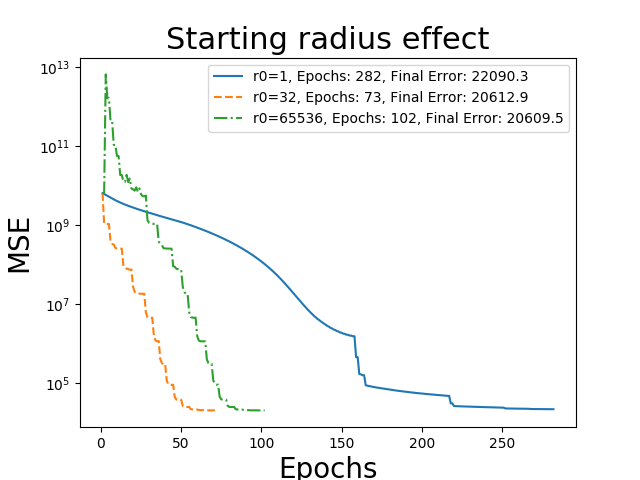
An important parameter for our algorithm is the starting radius $r^{(0)}$. This parameter controls how broad the search will be initially and has an effect similar to the learning rate of gradient-based optimization algorithms. If we are too conservative and choose a small initial radius, the algorithm will converge slowly to a local optimum, whereas if we set it too high, the error will overshoot and convergence is not guaranteed. A simple technique to automatically find a good starting radius is to use binary search. In particular, we set the starting radius to an arbitrary value, perform a dry run of the algorithm for one epoch and observe the effect on error. If the error increases we halve the radius. Otherwise we double it and repeat the process. This process is allowed to run for a small number of epochs. The starting radius found using this technique is a not too pessimistic or too optimistic estimate of the best parameter value.

4.2.4 Parallelization

Another way to boost the execution time is to utilize parallel computation to speed up parts of the algorithm. In our case we can parallelize the search for the optimal moves across the embedding dimensions using the map-reduce parallelization pattern. Specifically, we can map the search for candidate moves to run in different threads and store the error for each candidate move in an array $\mathbf{e}=[e_{1},e_{2}..,e_{2L}]$. After the search completes we can perform a reduction operation (min) to find the optimal move and the optimal error $\mathbf{X}^{*},e^{*}$. For our implementation we used the OpenMP parallelization framework [56] and it led to a $2-4$ times speedup in execution time.

4.2.5 Complexity

For each epoch we search across $2L$ dimensions for $N$ points. In each search we also need $\mathcal{O}(N)$ operations to update the distance matrix. Thus, the per epoch computational complexity of the algorithm is $\mathcal{O}(N^{2}L)$. The optimizations proposed above do not change the complexity of the algorithm per epoch with the notable exception of the move selection optimization: if instead of 2$L$ moves per epoch one would consider only 2$K$ moves. In this case, the overall complexity per epoch would be $\mathcal{O}(N^{2}K)$ instead of $\mathcal{O}(N^{2}L)$. However, as we shall see in the experiments that follow the (rest of the) proposed optimization significantly improve convergence speed, resulting in fewer epochs and less computation complexity overall.

4.3 GPS formulation of our Algorithm

Pattern Search MDS belongs to the general class of GPS methods and can be expressed using the unified GPS formulation introduced in Section 3.5. Next, we express our proposed algorithm and associated objective function under this formalism.

First, we restate the problem of MDS in a vectorized form. We use matrix $\mathbf{\Delta}$ with elements $\{\delta_{ij}\}_{1\leq i,j\leq N}$ that expresses the dissimilarities between $N$ points in the high dimensional space. The set of points $\{\mathbf{x}_{i}\}_{i=1}^{N}$ lie on the low dimensional manifold $\mathcal{M}\in\mathbb{R}^{L}$ and form the column set of matrix $\mathbf{X}^{T}$. The matrix $\mathbf{X}\in\mathbb{R}^{N\times L}$ will be now vectorized as an one column vector as shown next:

$$\begin{gathered}\mathbf{x}_{i}=[x_{i1},...,x_{iL}]^{T}\in\mathbb{R}^{L},1\leq i\leq N\\ \mathbf{z}=vec(\mathbf{X}^{T})=[x_{11},...,x_{1L},...,x_{N1},...,x_{NL}]^{T}\end{gathered}$$ (19)

Now our new variable $\mathbf{z}$ lies in the search space $\mathbb{R}^{N\cdot L}$. The distance between any two points $\mathbf{x}_{i}$ and $\mathbf{x}_{j}$ of the manifold $\mathcal{M}$ remains the same but is now expressed as a function of the vectorized variable $\mathbf{z}$. Namely, $d_{ij}(\mathbf{X})=||\mathbf{x}_{i}-\mathbf{x}_{j}||=\sqrt{\sum_{k=1}^{L}(x_{ik}-x_{jk})^{2}}=d_{ij}(\mathbf{z})$. To this end, our new objective function to minimize $g$ is the MSE between the given dissimilarities $\delta_{ij}$ and the euclidean distances $d_{ij}$ in the low dimensional manifold $\mathcal{M}$ as defined in Eq. 20 shown next:

$$g(\mathbf{z})=\frac{1}{N^{2}}\sum_{i=1}^{N}\sum_{j=1}^{N}(d_{ij}(\mathbf{z})-\delta_{ij})^{2},\enskip\mathbf{z}\in\mathbb{R}^{N\cdot L}$$ (20)

Consequently, the initial MDS is now expressed as an unconstrained non-convex optimization problem which is expressed by minimizing the function $g$ over the search space of $\mathbb{R}^{N\cdot L}$ (Eq. 21). Specifically, the $L$ coordinates for all $N$ points on the manifold $\mathcal{M}$ now serve as degrees of freedom for our solution.

$$\mathbf{z}^{*}=\underset{\mathbf{z}\in\mathbb{R}^{N\cdot L}}{\min}g(\mathbf{z})$$ (21)

Now that we have formulated the problem and the variable $\mathbf{z}$ in the appropriate format we can match each epoch of our initial algorithm with an iteration of a GPS method. Therefore, the moves produced by our algorithm form a sequence of points $\{\mathbf{z}^{(k)}\}$. Moreover, we are going to define the matrices $\mathbf{B},\mathbf{C}^{(k)},\mathbf{P}^{(k)}$ for our algorithm as in Eqs. 12, 13. The choice of our basis matrix $\mathbf{B}$ is the identity matrix as shown in Eq. 23.

$$\mathbf{e}_{i}=\underset{index\enskip i}{[0,..,\underbrace{1},...,0]}^{T},1\leq i\leq N\cdot L$$ (22)

$$\mathbf{B}=\mathbf{I}_{N\cdot L}=[\mathbf{e}_{1},...,\mathbf{e}_{N\cdot L}]$$ (23)

While the identity matrix is non singular and its columns span positively the search space $\mathbb{R}^{N\cdot L}$, we also define $\mathbf{M}^{(k)}$ as the identity matrix. In Eq. 24 matrix $\mathbf{\Gamma}^{(k)}$ represents the movement alongside the unit coordinate vectors of $\mathbb{R}^{N\cdot L}$. Nevertheless, our generating matrix $\hat{\mathbf{C}}$ also comprises of all the remaining possible directions which are generated by the set $\{-1,0,1\}$. In total, we have $3^{N\cdot L}-2\cdot N\cdot L$ extra direction vectors inside the corresponding matrix $\mathbf{L}^{(k)}$ as it is shown in Eq. 25.

$$\begin{gathered}\mathbf{M}^{(k)}=\hat{\mathbf{M}}=\mathbf{I}_{N\cdot L}\in\mathbb{Z}^{N\cdot L\times N\cdot L}\\ \mathbf{\Gamma}^{(k)}=\hat{\mathbf{\Gamma}}=[\hat{\mathbf{M}}\enskip-\hat{\mathbf{M}}]\end{gathered}$$ (24)

$$\begin{gathered}\hat{S}=\{-1,0,1\}\\ \mathbf{L}^{(k)}=\hat{\mathbf{L}}\\ \hat{\mathbf{L}}=\{\hat{v}:\hat{v}\in\underset{N\cdot L}{\underbrace{\hat{S}\times...\times\hat{S}}}\land\hat{v}\notin\{\mathbf{e}_{1},...,\mathbf{e}_{N\cdot L}\}\}\end{gathered}$$ (25)

According to Eqs. 24, 25, we construct the full pattern matrix $\mathbf{P}^{(k)}$ in Eq. 26 in a similar way to Eq. 13. For our algorithm the pattern matrix is is equal to our generating matrix $\mathbf{C}^{(k)}=\hat{\mathbf{C}}$ which is also fixed for all iterations. Conceptually, the generating matrix $\hat{\mathbf{C}}$ contains all the possible exploratory moves while a heuristic is utilized for evaluating the objective function $g$ only for a subset of them.

$$\begin{gathered}\mathbf{C}^{(k)}=\hat{\mathbf{C}}=[\hat{\mathbf{\Gamma}}\enskip\hat{\mathbf{L}}]=[\hat{\mathbf{M}}\enskip-\hat{\mathbf{M}}\enskip\hat{\mathbf{L}}]\\ \mathbf{P}^{(k)}=\hat{\mathbf{P}}\equiv\mathbf{B}\hat{\mathbf{C}}\equiv\hat{\mathbf{C}}\end{gathered}$$ (26)

Finally, we configure the updates of the step length parameter for each class of both successful and unsuccessful iterations as they were previously described in Eqs. 15, 16, respectively. Recalling the notation of Section 3.5, $\hat{\mathbf{s}}^{(k)}$ is the step which is returned from our exploratory moves subroutine at $k$th iteration. For the successful iterates $g(\mathbf{z}^{(k)}+\hat{\mathbf{s}}^{(k)})<g(\mathbf{z}^{(k)})$ we do not further increase the length of our moves by limiting $\Lambda=\{1\}$ as follows:

$$\Delta^{(k+1)}=\Delta^{(k)},\enskip\;\mbox{if}\;\enskip f(\mathbf{z}^{(k)}+\hat{\mathbf{s}}^{(k)})<f(\mathbf{z}^{(k)})$$ (27)

Similarly, for the unsuccessful iterations $g(\mathbf{z}^{(k)}+\hat{\mathbf{s}}^{(k)})\geq g(\mathbf{z}^{(k)})$ we halve the distance by a factor of $2$ by setting $\theta=\frac{1}{2}$ as it is shown next:

$$\Delta^{(k+1)}=\frac{1}{2}\Delta^{(k)},\enskip\;\mbox{if}\;\enskip f(\mathbf{z}^{(k)}+\hat{\mathbf{s}}^{(k)})>=f(\mathbf{z}^{(k)})$$ (28)

A short description of our algorithm as a GPS method for solving the problem stated in Eq. 21 follows: In each iteration, we fix the optimal coordinate direction for each one of the points lying on the low dimensional manifold $\mathbf{x}_{i}\in\mathcal{M},\enskip 1\leq i\leq N$. For each internal iteration of Alg. 4, if the optimal direction produces a lower value for our objective function $g$ we accumulate this direction and move alongside this coordinate of the $\mathbb{R}^{N\cdot L}$. Otherwise, we remain at the same position. As a result, the exploration of coordinates for the new point $\mathbf{x}_{i+1}$ begins from this temporary position. This greedy approach provides a potential one-hot vector as described in Eq. 22 if the iterate is successful or otherwise, the zero vector $\mathbf{0}\in\mathbb{R}^{N\cdot L}$. The final direction vector $\hat{\mathbf{s}}^{(k)}$ for $k$th iteration is computed by summing these one-hot or zero vectors. At the $k$th iteration, the movement would be given by a scalar multiplication of the step length parameter $\Delta^{(k)}$ with the final direction vector in a similar way as defined in Eq. 14. This provides a simple decrease for the objective function $g$ or in the worst case represent a zero movement in the search space $\mathbb{R}_{N\cdot L}$. Regarding the movement across $\hat{\mathbf{s}}^{(k)}$, it is trivial to show that this reduction of the objective function $g$ is an associative operation. In other words, accumulating all best coordinate steps for each point $\{\mathbf{x}_{i}\}_{i=1}^{N}$ and performing the movement at the end of the $k$th iteration (as GPS method formulation requires) produces the same result as taking each coordinate step individually. Finally, pattern search MDS terminates when the step length parameter $\Delta^{(k)}$ becomes smaller than a predefined threshold.

4.4 Convergence of our Algorithm

Now that we have homogenized the notation framework as well as have expressed the proposed algorithm as a GPS method one can utilize the theorems stated in Section 3.6 to prove the convergence properties of the proposed algorithm.

First of all, the objective function $g$ is indeed continuously differentiable for all the values of the search space $\mathbb{R}^{N\cdot L}$ by its definition in Eq. 20. Moreover, the pattern matrix $\hat{\mathbf{P}}$ in Eq. 26 contains all the possible step vectors provided by our exploratory moves routine. Thus, all of our exploratory moves are defined by Eq. 14. In each iteration we evaluate the trial steps alongside all coordinates for all the points $\mathbf{x}_{i}\in\mathcal{M},\enskip 1\leq i\leq N$. In our restated problem definition (see Section 4.3), this is translated to searching all over the identity matrices $\mathbf{I}_{N\cdot L}$ and $-\mathbf{I}_{N\cdot L}$ of the search space $\mathbb{R}^{N\cdot L}$. But from our definition of the first columns of our generating matrix in Eq. 24 this corresponds to checking all the potential coordinate steps provided by $\hat{\mathbf{\Gamma}}=[\mathbf{I}_{N\cdot L}\enskip-\mathbf{I}_{N\cdot L}]$. Consequently, if there exists a simple decrease when moving towards any of the directions provided by the columns of $\hat{\mathbf{\Gamma}}$ then our algorithm also provides a simple decrease. This result verifies that Hyp. 1 is true for the exploratory moves. By combining the differentiability of our objective function $g$ and Hyp. 1, Thm. 1 holds for pattern search MDS. Hence, $\underset{k\rightarrow+\infty}{\lim}\inf\;||\nabla f(\mathbf{z}^{(k)})||=0$ is guaranteed.

Trying to further strengthen the convergence properties of the proposed algorithm, we note that most of the requirements of Thm. 2 are met but we fail to meet the specifications of Hyp. 2 for the minimum decrease provided by the the columns of $\hat{\mathbf{\Gamma}}$. However, our generating matrix $\hat{\mathbf{C}}=[\hat{\mathbf{c}}_{1},...,\hat{\mathbf{c}}_{3^{N\cdot L}}]$ is indeed bounded by norm because $||\hat{\mathbf{c}}_{j}||_{1}\leq N\cdot L,\enskip 1\leq j\leq 3^{N\cdot L}$. By halving the step length parameter for the unsuccessful iterations we also ensure that $\lim_{k\rightarrow\infty}\Delta^{(k)}$. In order to meet the specifications of Thm. 2 we would need a quadratic complexity of $\mathcal{O}((N\cdot L)^{2})$ in order to ensure that each iteration provides the same decrease in function $g$ as the decrease provided by the “best” column of $\hat{\mathbf{\Gamma}}$. This is formally stated at the second part of Hyp. 2. If we modify our algorithm in order to meet these requirements we would not be able to implement all the optimizations proposed in Section 4.2 and the overall runtime would be dramatically increased.

5 EXPERIMENTS

5.1 Tuning the hyperparameters

Next we present some guidelines on how to set the hyperparameters for the proposed algorithm and report the values used in the experiments that follow. Specifically:

• The constant $\epsilon$ in line 9 of Alg. 2 determines when the move radius $r$ is decreased. By setting $\epsilon$ to a value very close to $0$, e.g., $10^{-10}$, the search will take more epochs but the solution will be closer to the local optimum. If we relax $\epsilon$ to a value around $10^{-2}$, we can do a coarse exploration of the search space that will produce a rough solution in a small number of epochs. In our experiments we set $\epsilon=10^{-4}$ that provides a good trade-off between solution quality and fast convergence for the datasets used.

• We experimentally found that if $L$ is large, we may only search $50\%$ of the search dimensions and still get a good solution, while significantly reducing the execution time. For this to hold, it is important that we randomly sample a new search space for each epoch.

• The proposed algorithm is relatively robust to the choice of the initial size of the move search radius. However, the choice of $r^{(0)}$ does affect convergence speed. We show the convergence for an example run of the classical swissroll (see Section 5.2) for best-case ($r^{(0)}=32$), pessimistic ($r^{(0)}=1$) and optimistic ($r^{(0)}=65536$) starting radii in Fig. 2.

Figure 2: Convergence plot for different starting radii

5.2 Manifold Geometry

The key assumption in manifold learning is that input data lie on a low-dimensional, non-linear manifold, embedded in a high-dimensional space. Thus non-linear dimensionality reduction techniques aim to extract the low-dimensional manifold from the high dimensional space. To showcase this we generated a variety of geometric manifold shapes and compared the proposed MDS to other, well-established dimensionality reduction techniques. We make the code to generate the synthetic data openly available to the community.

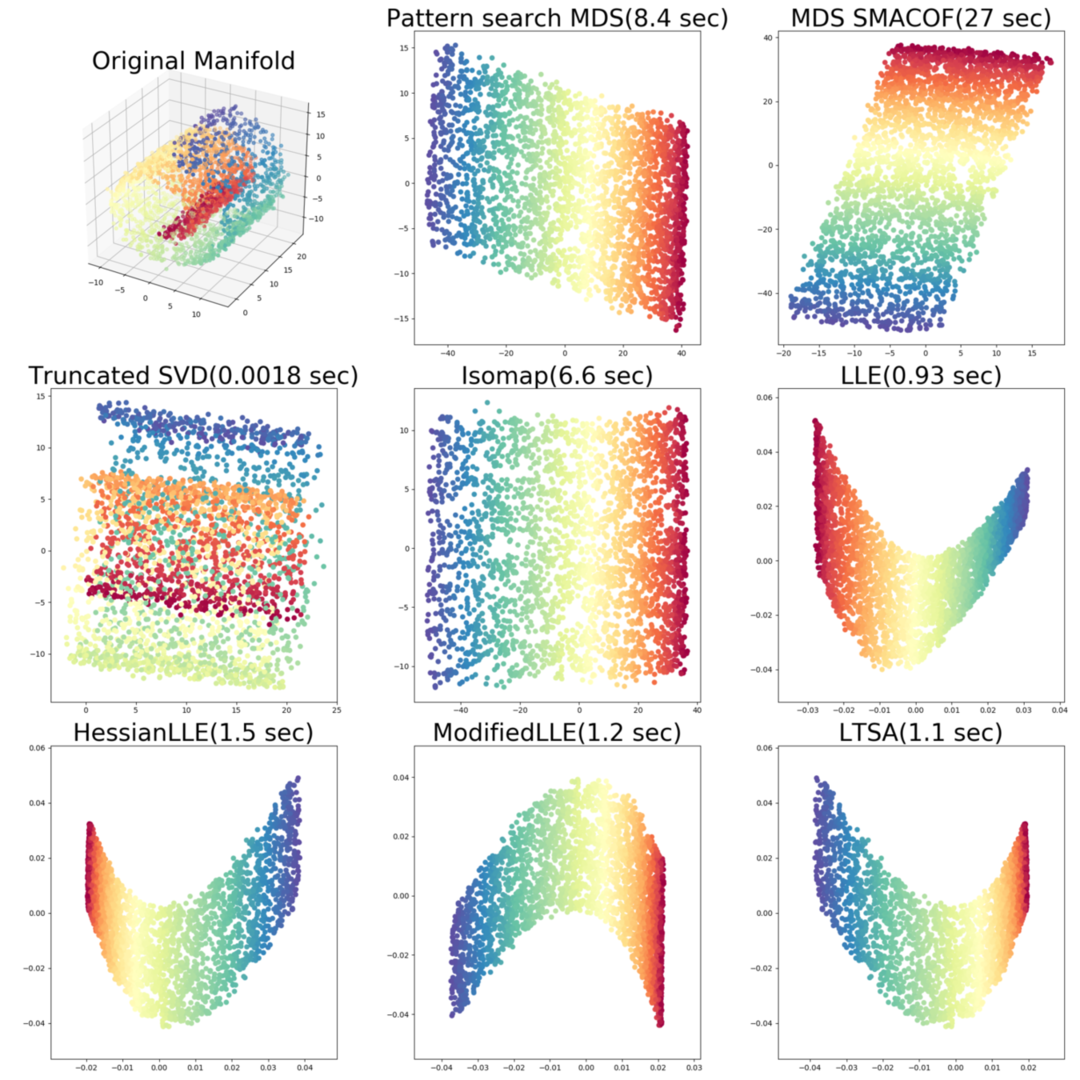
One should note that MDS algorithms with Euclidean distance matrices as inputs cannot infer data geometry, thus we need to provide as input a geodesic distance matrix. This matrix is computed by running Djikstra’s shortest path algorithm on the Nearest Neighbors graph trained on the input data. For our experiments we sample $3000$ points on $11$ $3D$ shapes and reduce them to $2$ dimensions using pattern search MDS, SMACOF MDS [52], truncated SVD [57], Isomap [6, 7, 8, 9, 10], Local Linear Embedding (LLE) [13, 14, 15, 16, 17], Hessian LLE [19, 20], modified LLE [18] and Local Tangent Space Alignment (LTSA) [27].

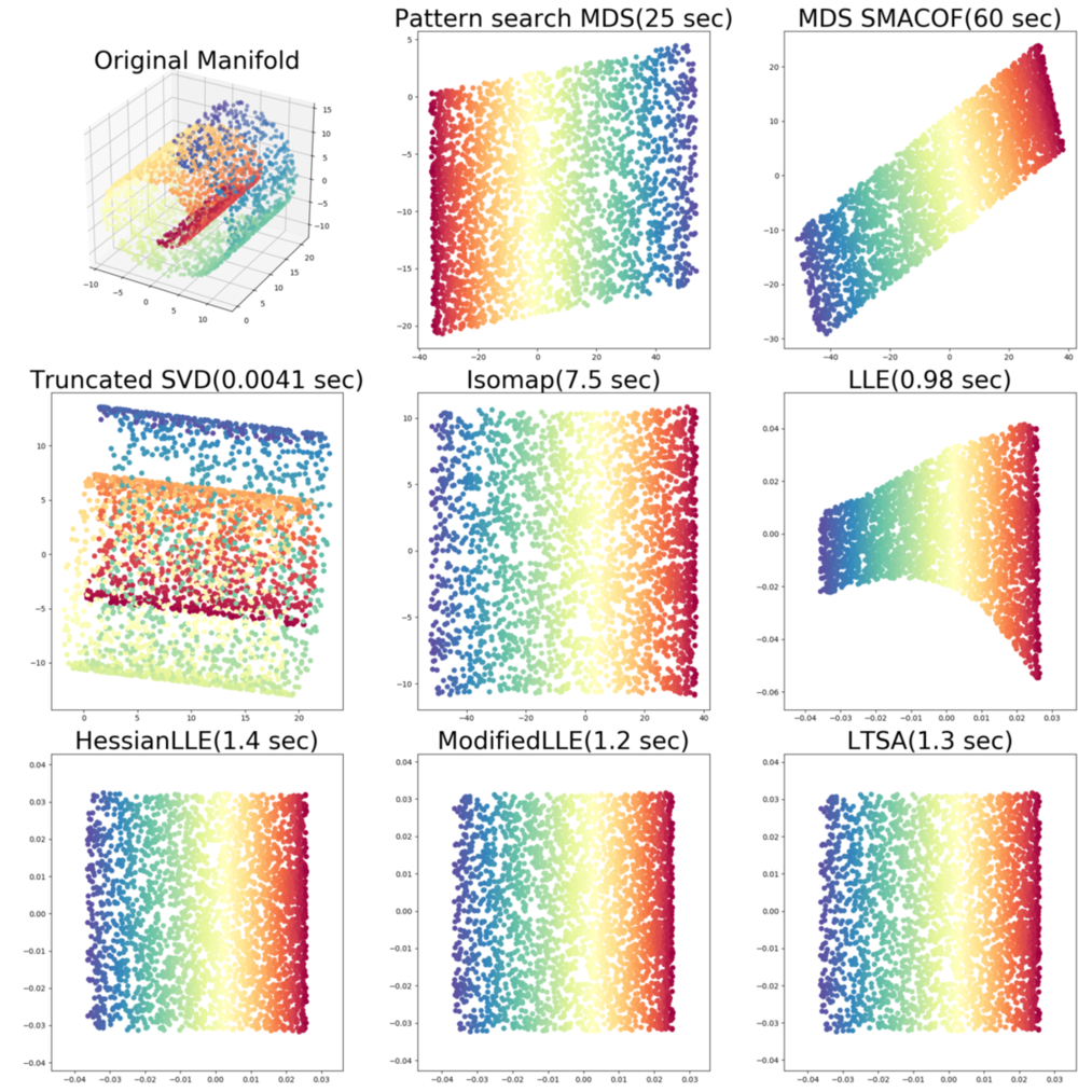
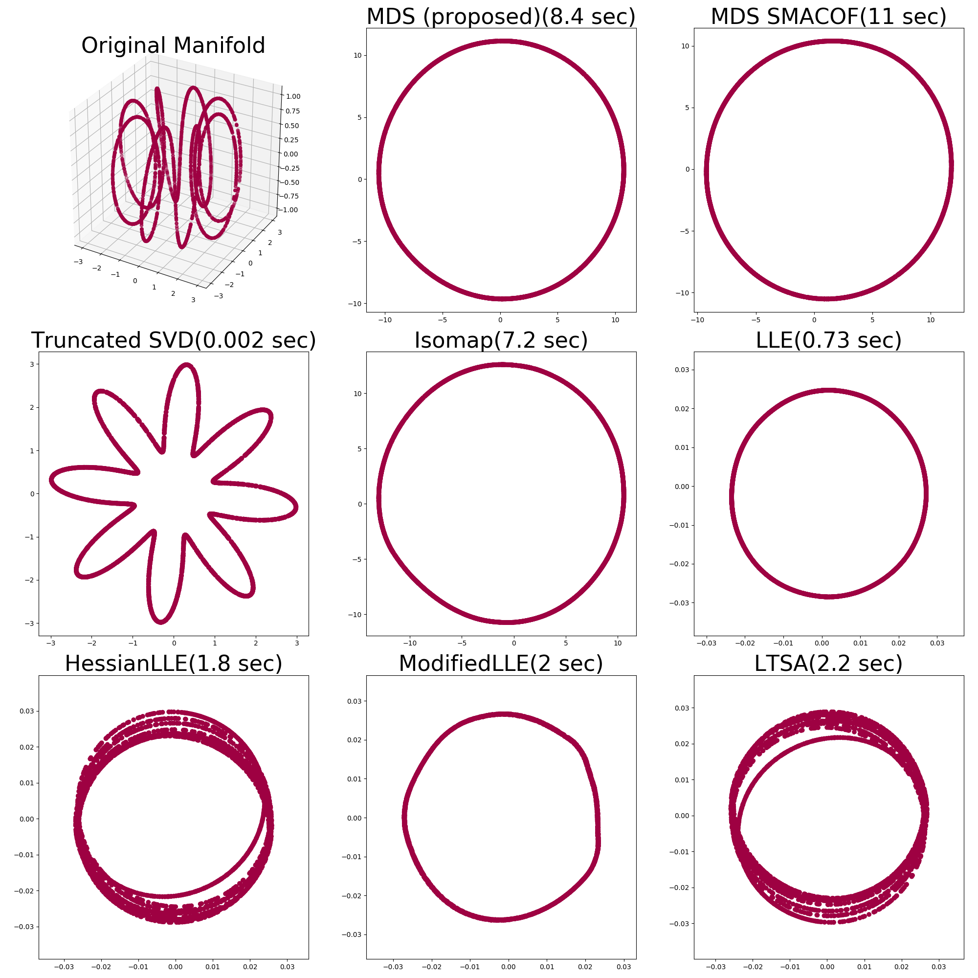
The geodesic distance matrices provided to pattern search MDS and SMACOF MDS is computed using Djikstra’s algorithm on k-NN (nearest neighbor) graphs. We list the times it took each method to run. Note that pattern search MDS is faster than SMACOF MDS.

We present $3$ characteristic shapes selected from the ones we tested. The first shape we examine is the classical swissroll, where a $2D$ plane is “rolled” in $3D$ space and the target is to extract the original $2D$ plane. Results are presented in Fig. 3(a). We observe that linear dimensionality reduction techniques like truncated SVD have trouble unrolling the swissroll. Also LLE introduces a lot of distortion to the constructed plane.

(a)

(b)

(c)

Figure 3: Comparison of pattern search MDS with other dimensionality reduction methods when converting: (3(a)) $3D$ swissroll to $2D$ plane, (3(b)) $3D$ clusters to $2D$ clusters, and (3(c)) $3D$ toroid helix to $2D$ circle

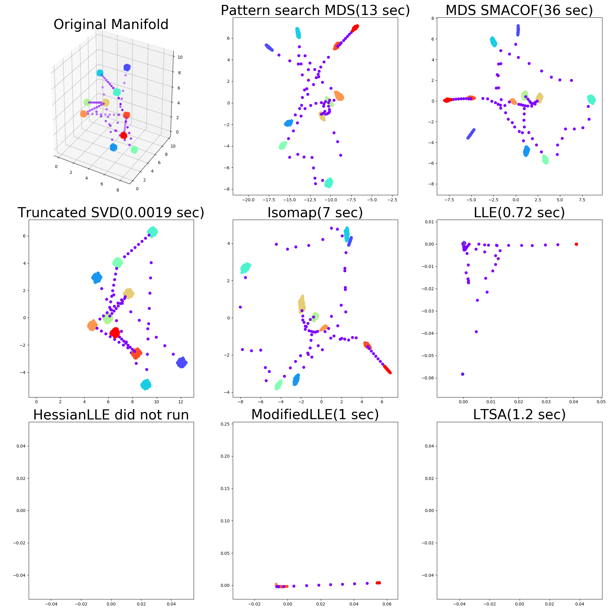
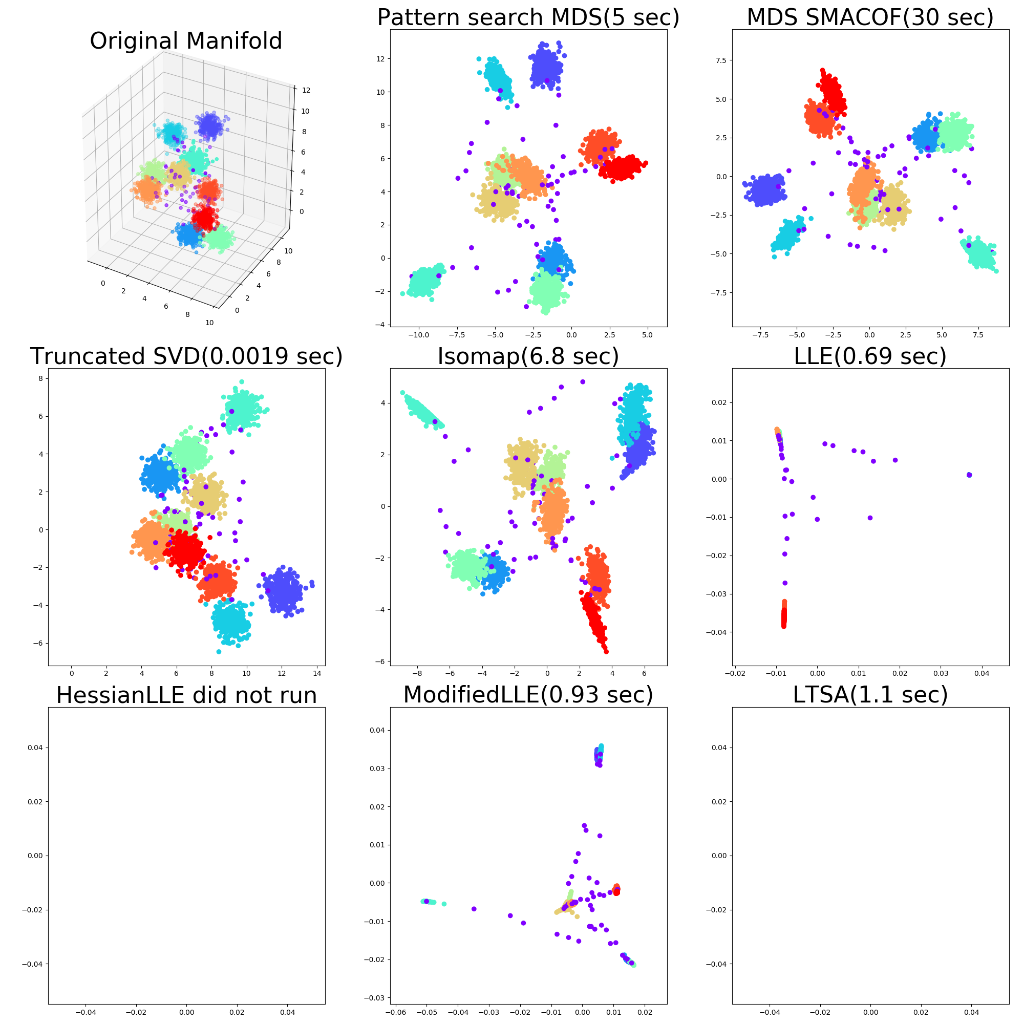
Next we examine how the algorithms handle sparse distance matrices. To this end, we generate a dataset of $3D$ non-overlapping clusters with a line connecting the centroids, where sparsity of the distance matrix follows because the vast majority of the points are very closely sampled inside the clusters. A good mapping should preserve the cluster structure in lower dimensions. In Fig. 3(b) we see that the truncated SVD and the MDS family of algorithms (proposed, SMACOF, Isomap) produce good results, while the LLE variants can’t handle sparsity in distance matrices very well. In particular Hessian LLE and LTSA do not produce any output because of numerical instability in the eigenvalue decomposition stages of these algorithms. Pattern search MDS does not rely on eigenvalue computation or equation system solvers and therefore it is numerically stable.

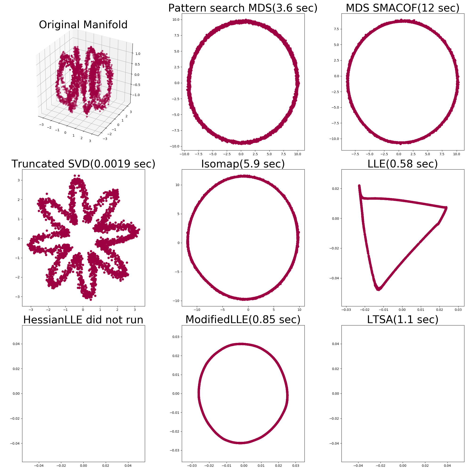
Finally, we showcase how the algorithms perform with transitions from dense to sparse regions with a toroidal helix shape in Fig. 3(c). We can see that five methods, including pattern search MDS, unroll the shape into the expected $2D$ circle, while truncated SVD provides a daisy-like shape. Hessian LLE and LTSA collapse the helix into multiple overlapping circles.

5.3 Dimensionality reduction for semantic similarity

Construction of semantic network models consists of representing concepts as vectors in a, possibly high-dimensional, space $\mathbb{R}^{n}$. The relations between concepts are quantified as the distances, or inversely the cosine similarities, between semantic vectors. The semantic similarity task aims to evaluate the correlation of the similarities between concepts in a given semantic space against a set of ground truth similarity values provided by human annotators.

We evaluate the performance of the dimensionality techniques investigated also in Section 5.2 for the semantic similarity task. We use the MEN [58] and SimLex-999 [59] semantic datasets as ground truth. Both datasets are provided in the form of lists of word pairs, where each pair is associated with a similarity score. This score was computed by averaging the similarities provided by human annotators. As the high-dimensional semantic word vectors, we use the $300$-dimensional GloVe vectors constructed by [60] using a large Twitter corpus. We reduce the dimensionality of the vectors to the target dimension $L$ and calculate the Spearman correlation coefficient between the human provided and the automatically computed similarity scores. Results are summarized in Table 1 for $L=10$. We observe that LLE yields the best results for MEN, while pattern search MDS performs best for SimLex-999. In addition, we observe that non-linear dimensionality reduction techniques can significantly improve the performance of the semantic vectors in some cases.

Dimensionality reduction	Dimensions	MEN	SimLex-999
-	$300$	$0.635$	$0.177$
pattern search MDS	$10$	$0.596$	0.242
MDS SMACOF	$10$	$0.632$	$0.221$
Isomap	$10$	$0.625$	$0.132$
Truncated SVD	$10$	$0.562$	$0.140$
LLE	$10$	0.657	$0.172$
Hessian LLE	$10$	$0.157$	$0.004$
Modified LLE	$10$	$0.643$	$0.158$
LTSA	$10$	$0.154$	$0.004$

Table 1: Comparison of dimensionality reduction techniques for the semantic similarity task for MEN and SimLex-999 datasets.

5.4 Dimensionality reduction for k-NN classification

The next set of experiments aims to compare the proposed algorithm to other dimensionality reduction methods for k-NN classification on a real dataset. We choose to use MNIST as a benchmark dataset which contains $70,000$ handwritten digit images. We selected a random subset of $1000$ images and reduced the dimensionality from $784$ to $20$. Performance of the models is evaluated on 1-NN classification and using $10$-fold cross-validation. The evaluation metric is macro-averaged F1 score. Table 2 summarizes the results. Observe that dimensionality reduction using pattern search MDS and Truncated SVD can improve classification performance over the original high-dimensional data. Pattern search MDS yields the best results overall. Hessian LLE, Modified LLE and LTSA did not run due to numerical instability.

Method	Dimensions	MNIST 1-NN F1 score
Original MNIST	$784$	$0.861$
pattern search MDS	$20$	0.878
MDS SMACOF	$20$	$0.857$
Isomap	$20$	$0.829$
Truncated SVD	$20$	$0.871$
LLE	$20$	$0.813$
Hessian LLE	$20$	$-$
Modified LLE	$20$	$-$
LTSA	$20$	$-$

Table 2: Comparison of dimensionality reduction techniques for the MNIST dataset.

5.5 Convergence characteristics

Next we compare speed of convergence of pattern search MDS and MDS SMACOF, in terms of numbers of epochs. To this end we will consider the experiments of Sections 5.2 and 5.3 and present comparative convergence plots. We see the convergence plots for the cases of swissroll, $3D$ clusters, toroid helix in Fig. 4(a), 4(b) and 4(c), respectively. The convergence plot for the word semantic similarity task is shown in Fig. 4(d). The plots are presented in y-axis logarithmic scale because the starting error is many orders of magnitude larger than the local minimum reached by the algorithms.

(a)

(b)

(c)

(d)

Figure 4: Convergence comparison of pattern search MDS and MDS SMACOF for (4(a)) swissroll, (4(c)) toroid helix, (4(b)) 3d clusters and (4(d)) word vectors

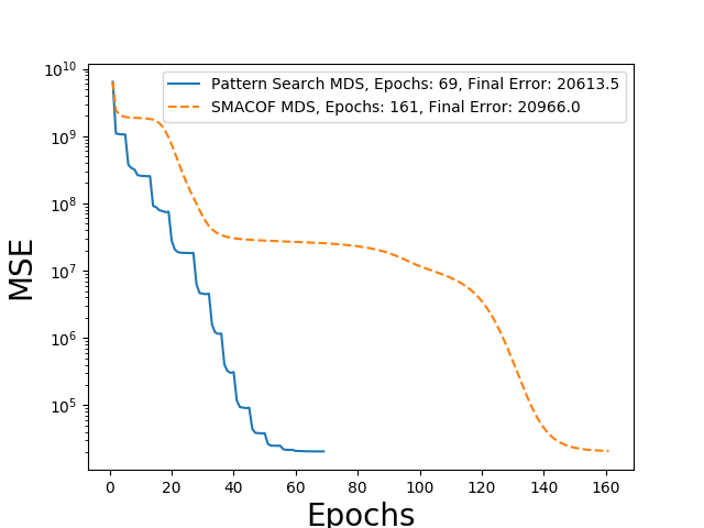
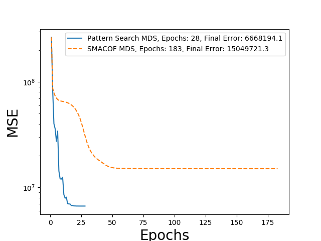
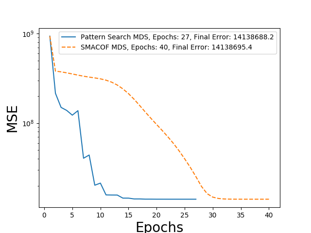
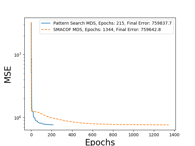
For all cases, we observe that pattern search MDS converges very quickly to a similar or better local optimum while MDS SMACOF hits regions where the convergence slows down and then recovers. These saw-like structure of the pattern search plots are due to the fact that we allow for “bad moves” as detailed in Section  4.2.1.

5.6 Robustness to noisy or missing data

The final set of experiments aims to demonstrate the robustness of pattern search MDS when the input data are corrupted or noisy. To this end two cases of data corruption are considered: additive noise and missing data.

5.6.1 Robustness to additive noise

For this set of experiments, we inject Gaussian noise of variable standard deviation ($\sigma$) to the input data and use the dissimilarity matrix calculated on the noisy data as input to each one of the algorithms evaluated.

For the synthetic data of Section 5.2, we will follow a qualitative evaluation by showing the unrolled manifolds for high levels of noise. We perform dimensionality reduction for swissroll, toroid helix and $3D$ clusters for increasing noise levels. We report results for the highest possible noise deviation where one or more techniques still produce meaningful manifolds. Beyond these values of $\sigma$ the original manifolds become corrupted and the output of all methods is dominated by noise. Figs. 5(a), 5(b), 5(c) show the results for noisy swissroll with $\sigma=0.3$, $3D$ clusters with $\sigma=0.4$ and toroid helix with $\sigma=0.07$ respectively. Overall, the pattern search MDS, followed by SMACOF MDS and Isomap are more robust to additive noise.

(a)

(b)

(c)

Figure 5: Comparison of pattern search MDS with other dimensionality reduction methods when converting noisy (3(a)) $3D$ swissroll to $2D$ plane ($\sigma=0.4$), (3(b)) $3D$ clusters to $2D$ clusters ($\sigma=0.3$) and (3(c)) $3D$ toroid helix to $2D$ circle ($\sigma=0.07$)

For the semantic similarity task we injected different levels of Gaussian noise in the original word vectors and evaluated the correlation on MEN and Simlex-999. Results are presented in Table 3. We observe that the relative performance of the algorithms is maintained under noise injection, except for LLE which cannot handle high amounts of noise. LLE is achieving the best correlation values on MEN at $\sigma=0.01$ and $\sigma=0.1$, while pattern search MDS achieving the best performance on Simlex-999.

Method	Dimensions	MEN			SimLex-999
		$\sigma=0.01$	$\sigma=0.1$	$\sigma=0.5$	$\sigma=0.01$	$\sigma=0.1$	$\sigma=0.5$
Original GloVe	$300$	$0.635$	$0.619$	$0.431$	$0.178$	$0.169$	$0.077$
pattern search MDS	$10$	$0.593$	$0.597$	$0.462$	0.249	0.315	0.204
MDS SMACOF	$10$	$0.633$	$0.620$	$0.462$	$0.229$	$0.222$	$0.123$
Isomap	$10$	$0.622$	$0.613$	0.497	$0.134$	$0.124$	$0.079$
Truncated SVD	$10$	$0.562$	$0.551$	$0.380$	$0.140$	$0.136$	$0.039$
LLE	$10$	0.659	0.649	$0.369$	$0.175$	$0.166$	$0.052$
Hessian LLE	$10$	$0.156$	$0.144$	$0.023$	$0.005$	$0.04$	$0.018$
Modified LLE	$10$	$0.635$	$0.633$	$0.489$	$0.158$	$0.162$	$0.096$
LTSA	$10$	$0.155$	$0.141$	$0.020$	$0.06$	$0.04$	$0.002$

Table 3: Comparison of dimensionality reduction techniques with noisy word vectors on the semantic similarity task for MEN and SimLex-999 datasets.

5.6.2 Robustness to missing data

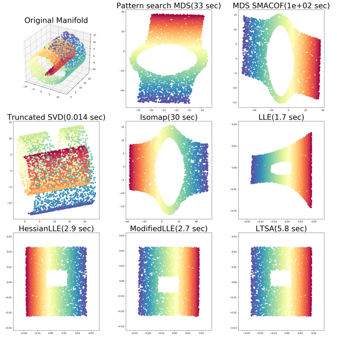
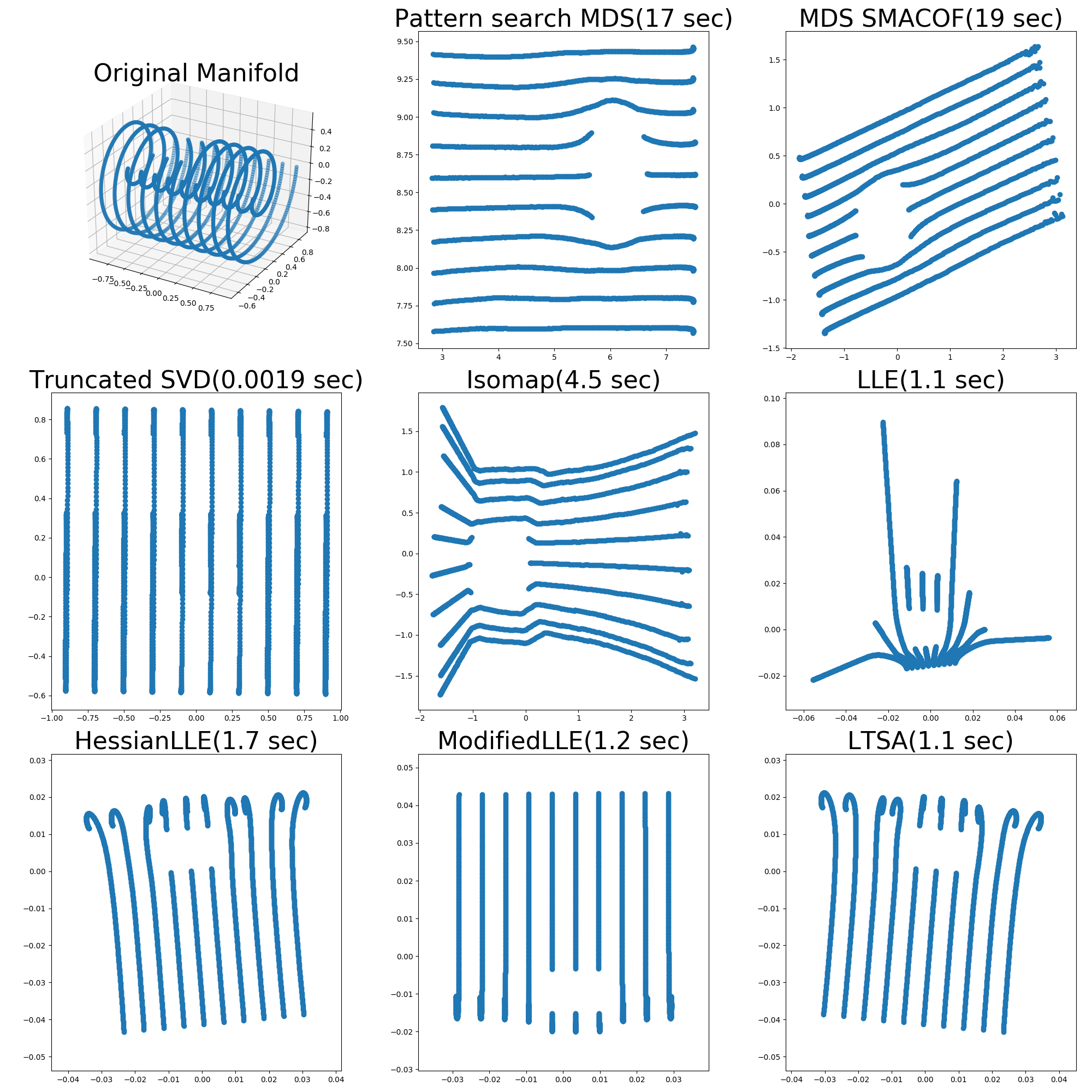
For the final set of experiments we consider the case of missing data. For this two new synthetic datasets where constructed, namely a dense and a sparse swissroll with a hole as shown in Fig. 6. In Fig 6(a), we show the performance of the various algorithms applied to a dense swissroll with a hole in the middle. As we can see only Hessian LLE, modified LLE and LTSA are able to reconstruct the shape correctly, while MDS algorithms result in distortion around the hole. This is due to the non-convexity we introduced to the space when adding the hole. This distortion can still be observed (to a lesser degree) in the sparse variation shown in Fig. 6(b). For the sparse data case, we observe that LLE methods result in distortion around the edges.

These preliminary experiments indicate that LLE variations can handle better non-convexities in input data, while MDS variations can handle sparse data better. This is because LLE methods are based on inferring and combining local data geometry, while MDS methods are inferring global geometry.

(a)

(b)

Figure 6: Comparison of pattern search MDS with other dimensionality reduction methods for (6(a)) dense and (6(b)) sparse swissroll with hole. Target is a plane with a rectangular hole.

6 CONCLUSIONS

We propose pattern search MDS, a novel algorithm for nonlinear dimensionality reduction, inspired by gradient-free optimization methods. Pattern search MDS is formulated as an instance of the wider family of GPS methods, thus providing theoretical guarantees of convergence up to a fixed point. Additional optimizations further improve the performance of our algorithm in terms of computational efficiency, robustness and solution quality. The qualitative evaluation against other popular dimensionality reduction techniques for both clean and noisy manifold geometry shapes indicates that pattern search MDS can accurately infer the intrinsic geometry of manifolds embedded in high-dimensional spaces. Furthermore, the comparison of convergence characteristics against SMACOF MDS show that pattern search MDS converges in fewer epochs to similar or better solutions. Experiments on real data yield comparable to state-of-the-art results both for a lexical semantic similarity task and on MNIST for KNN classification. Open-source implementations of pattern search MDS and the data generation process are provided to facilitate the reproducibility of our results.

7 FUTURE WORK

Future work will focus on improving runtime performance and scalability of pattern search MDS. Specifically, an approach for decreasing per epoch computational complexity is to narrow the search space of possible moves as the geometry of the embedding space becomes more apparent by biasing the moves towards the principal component vectors of the neighborhood of the point that is being moved. This can be viewed as a combination of pattern search and gradient descent, where the search space of moves is wide at the beginning and then gets increasingly biased towards the direction of the gradient. Our algorithm can scale to large numbers of points by utilizing Landmark points [11] or fast approximations to MDS [61]. These approaches aim to alleviate the computational and memory cost of computing the full distance matrix, by approximating the data geometry using smaller submatrices. Moreover, stochastic approximations like stochastic SMACOF [62] can be adapted to pattern search MDS.

We also plan to provide more in-depth theoretical insights and ways to enable pattern search MDS to capture complex geometrical properties of input data. We aim to perform a detailed analysis on how heuristics and especially allowing for “bad moves” affect the performance of pattern search MDS. Furthermore, in Sections 5.2 and 5.6.2 we showcased that MDS can better handle sparse data and LLE can better handle non-convexity and missing data. This makes sense, as MDS takes into account the global geometry of the embedding space, while LLE focuses on the geometry of local neighborhoods. We plan to combine the cost functions of these approaches to infer both global and local geometry of the low dimensional data manifold. Another way to increase the expressiveness of the algorithm is to investigate a wider variety of distance metrics, and specifically non-symmetrical distance “metrics”, motivated by cognitive sciences [3].

References

- [1] Charles Fefferman, Sanjoy Mitter and Hariharan Narayanan “Testing the manifold hypothesis” In Journal of the American Mathematical Society 29.4, 2016, pp. 983–1049
- [2] Pentti Kanerva “Sparse distributed memory” MIT press, 1988
- [3] Emmanuel Pothos and Jerome Busemeyer “A quantum probability explanation for violations of symmetry in similarity judgments” In Proceedings of the Annual Meeting of the Cognitive Science Society 33.33, 2011
- [4] Emmanuel M Pothos and Jerome R Busemeyer “Can quantum probability provide a new direction for cognitive modeling?” In Behavioral and Brain Sciences 36.3 Cambridge University Press, 2013, pp. 255–274
- [5] Karl F.R.S. Pearson “LIII. On lines and planes of closest fit to systems of points in space” In The London, Edinburgh, and Dublin Philosophical Magazine and Journal of Science 2.11 Taylor & Francis, 1901, pp. 559–572
- [6] Joshua B. Tenenbaum, Vin de Silva and John C. Langford “A Global Geometric Framework for Nonlinear Dimensionality Reduction” In Science 290.5500 American Association for the Advancement of Science, 2000, pp. 2319–2323
- [7] Mira Bernstein, Vin De Silva, John C. Langford and Joshua B. Tenenbaum “Graph Approximations to Geodesics on Embedded Manifolds”, 2000
- [8] Hongyuan Zha and Zhenyue Zhang “Isometric embedding and continuum ISOMAP” In Proceedings of the 20th International Conference on Machine Learning (ICML-03), 2003, pp. 864–871
- [9] David L. Donoho and Carrie Grimes “Image Manifolds which are Isometric to Euclidean Space” In Journal of Mathematical Imaging and Vision 23.1, 2005, pp. 5–24
- [10] Robert Pless “Image Spaces and Video Trajectories: Using Isomap to Explore Video Sequences.” In ICCV 3, 2003, pp. 1433–1440
- [11] Vin Silva and Joshua B. Tenenbaum “Sparse Multidimensional Scaling using Landmark Points” In Technology, 2004
- [12] Vin De Silva and Joshua B. Tenenbaum “Global versus local methods in nonlinear dimensionality reduction” In Advances in Neural Information Processing Systems 15 MIT Press, 2003, pp. 705–712
- [13] Mikhail Belkin and Partha Niyogi “Laplacian Eigenmaps for Dimensionality Reduction and Data Representation” In Neural Comput. 15.6 Cambridge, MA, USA: MIT Press, 2003, pp. 1373–1396
- [14] Lawrence Cayton and Sanjoy Dasgupta “Robust Euclidean Embedding” In Proceedings of the 23rd International Conference on Machine Learning, ICML ’06 Pittsburgh, Pennsylvania, USA: ACM, 2006, pp. 169–176
- [15] Lawrence K. Saul and Sam T. Roweis “Think Globally, Fit Locally: Unsupervised Learning of Low Dimensional Manifolds” In J. Mach. Learn. Res. 4 JMLR.org, 2003, pp. 119–155
- [16] Fei Sha and Lawrence K. Saul “Analysis and Extension of Spectral Methods for Nonlinear Dimensionality Reduction” In Proceedings of the 22Nd International Conference on Machine Learning, ICML ’05 Bonn, Germany: ACM, 2005, pp. 784–791
- [17] Mikhail Belkin and Partha Niyogi “Laplacian Eigenmaps and Spectral Techniques for Embedding and Clustering” In Advances in Neural Information Processing Systems 14 MIT Press, 2002, pp. 585–591
- [18] Zhenyue Zhang and Jing Wang “MLLE: Modified locally linear embedding using multiple weights” In Advances in neural information processing systems, 2007, pp. 1593–1600
- [19] Zhenyue Zhang and Hongyuan Zha “Principal manifolds and nonlinear dimensionality reduction via tangent space alignment” In SIAM journal on scientific computing 26.1 SIAM, 2004, pp. 313–338
- [20] David L. Donoho and Carrie Grimes “Hessian eigenmaps: Locally linear embedding techniques for high-dimensional data” In Proceedings of the National Academy of Sciences 100.10 National Academy of Sciences, 2003, pp. 5591–5596
- [21] Kilian Q Weinberger and Lawrence K Saul “Unsupervised learning of image manifolds by semidefinite programming” In International journal of computer vision 70.1 Springer, 2006, pp. 77–90
- [22] Kilian Q Weinberger, Benjamin Packer and Lawrence K Saul “Nonlinear Dimensionality Reduction by Semidefinite Programming and Kernel Matrix Factorization.” In AISTATS, 2005 Citeseer
- [23] Lieven Vandenberghe and Stephen Boyd “Semidefinite Programming” In SIAM Rev. 38.1 Philadelphia, PA, USA: Society for IndustrialApplied Mathematics, 1996, pp. 49–95
- [24] Dimitri P Bertsekas “Nonlinear programming” Athena scientific Belmont, 1999
- [25] Mikhail Belkin and Partha Niyogi “Laplacian eigenmaps and spectral techniques for embedding and clustering” In Advances in neural information processing systems, 2002, pp. 585–591
- [26] Mikhail Belkin and Partha Niyogi “Convergence of Laplacian Eigenmaps” In Advances in Neural Information Processing Systems 19 MIT Press, 2007, pp. 129–136
- [27] Zhenyue Zhang and Hongyuan Zha “Principal Manifolds and Nonlinear Dimensionality Reduction via Tangent Space Alignment” In SIAM J. Sci. Comput. 26.1 Philadelphia, PA, USA: Society for IndustrialApplied Mathematics, 2005, pp. 313–338
- [28] Bernhard Schölkopf, Alexander Smola and Klaus-Robert Müller “Nonlinear component analysis as a kernel eigenvalue problem” In Neural computation 10.5 MIT Press, 1998, pp. 1299–1319
- [29] Luis Miguel Rios and Nikolaos V. Sahinidis “Derivative-free optimization: a review of algorithms and comparison of software implementations” In Journal of Global Optimization 56.3, 2013, pp. 1247–1293
- [30] Mordecai Avriel “Nonlinear programming: analysis and methods” Courier Corporation, 2003
- [31] Robert Hooke and T. A. Jeeves ““ Direct Search” Solution of Numerical and Statistical Problems” In J. ACM 8.2 New York, NY, USA: ACM, 1961, pp. 212–229
- [32] George EP Box “Evolutionary operation: A method for increasing industrial productivity” In Applied statistics JSTOR, 1957, pp. 81–101
- [33] Virginia Joanne Torczon “Multidirectional search: a direct search algorithm for parallel machines”, 1989
- [34] Jr. J. E. Dennis and Virginia Torczon “Direct Search Methods on Parallel Machines” In SIAM Journal on Optimization 1.4, 1991, pp. 448–474
- [35] Virginia Torczon “On the convergence of pattern search algorithms” In SIAM Journal on optimization 7.1 SIAM, 1997, pp. 1–25
- [36] Elizabeth D Dolan, Robert Michael Lewis and Virginia Torczon “On the local convergence of pattern search” In SIAM Journal on Optimization 14.2 SIAM, 2003, pp. 567–583
- [37] Robert Michael Lewis and Virginia Torczon “Pattern Search Methods for Linearly Constrained Minimization” In SIAM Journal on Optimization 10.3, 2000, pp. 917–941
- [38] Robert Michael Lewis and Virginia Torczon “Pattern Search Algorithms for Bound Constrained Minimization” In SIAM Journal on Optimization 9.4, 1999, pp. 1082–1099
- [39] Andrew R. Conn, Nicholas I. M. Gould and Philippe Toint “A Globally Convergent Augmented Lagrangian Algorithm for Optimization with General Constraints and Simple Bounds” In SIAM Journal on Numerical Analysis 28.2, 1991, pp. 545–572
- [40] Warren S. Torgerson “Multidimensional scaling: I. Theory and method” In Psychometrika 17.4, 1952, pp. 401–419
- [41] Ingwer Borg and Patrick J. F. Groenen “Modern multidimensional scaling: theory and applications” Springer, 2005
- [42] J. C. Gower “Some distance properties of latent root and vector methods used in multivariate analysis” In Biometrika 53.3-4, 1966, pp. 325–338
- [43] M. A. A. Cox and T. F. Cox “Multidimensional Scaling on the Sphere” In Compstat Heidelberg: Physica-Verlag HD, 1988, pp. 323–328
- [44] Andrej Cvetkovski and Mark Crovella “Low-stress data embedding in the hyperbolic plane using multidimensional scaling” In Appl. Math 11.1, 2017, pp. 5–12
- [45] Harold Lindman and Terry Caelli “Constant curvature Riemannian scaling” In Journal of Mathematical Psychology 17.2 Elsevier, 1978, pp. 89–109
- [46] Roger N. Shepard “The analysis of proximities: Multidimensional scaling with an unknown distance function. I.” In Psychometrika 27.2, 1962, pp. 125–140
- [47] Roger N. Shepard “The analysis of proximities: Multidimensional scaling with an unknown distance function. II” In Psychometrika 27.3, 1962, pp. 219–246
- [48] PJ Groenen and Ingwer Borg “Past, present, and future of multidimensional scaling” In Visualization and Verbalization of Data CRC Press, 2014, pp. 95–117
- [49] J. B. Kruskal “Multidimensional scaling by optimizing goodness of fit to a nonmetric hypothesis” In Psychometrika 29.1, 1964, pp. 1–27
- [50] J. B. Kruskal “Nonmetric multidimensional scaling: A numerical method” In Psychometrika 29.2, 1964, pp. 115–129
- [51] Stephen L France and J Douglas Carroll “Two-way multidimensional scaling: A review” In IEEE Transactions on Systems, Man, and Cybernetics, Part C (Applications and Reviews) 41.5 IEEE, 2011, pp. 644–661
- [52] Jan De Leeuw et al. “Applications of convex analysis to multidimensional scaling” In Recent Developments in Statistics North Holland Publishing Company, 1977, pp. 133–146
- [53] Jan Leeuw “Convergence of the majorization method for multidimensional scaling” In Journal of Classification 5.2, 1988, pp. 163–180
- [54] Charles Audet “Convergence Results for Generalized Pattern Search Algorithms are Tight” In Optimization and Engineering 5.2, 2004, pp. 101–122
- [55] Scott Kirkpatrick, C Daniel Gelatt and Mario P Vecchi “Optimization by simulated annealing” In science 220.4598 American Association for the Advancement of Science, 1983, pp. 671–680
- [56] Leonardo Dagum and Ramesh Menon “OpenMP: an industry standard API for shared-memory programming” In IEEE computational science and engineering 5.1 IEEE, 1998, pp. 46–55
- [57] Gene Golub and William Kahan “Calculating the singular values and pseudo-inverse of a matrix” In Journal of the Society for Industrial and Applied Mathematics, Series B: Numerical Analysis 2.2 SIAM, 1965, pp. 205–224
- [58] Elia Bruni, Nam Khanh Tran and Marco Baroni “Multimodal Distributional Semantics” In J. Artif. Int. Res. 49.1 USA: AI Access Foundation, 2014, pp. 1–47
- [59] Felix Hill, Roi Reichart and Anna Korhonen “Simlex-999: Evaluating semantic models with (genuine) similarity estimation” In Computational Linguistics, 2015
- [60] Christos Baziotis, Nikos Pelekis and Christos Doulkeridis “DataStories at SemEval-2017 Task 4: Deep LSTM with Attention for Message-level and Topic-based Sentiment Analysis” In Proceedings of the 11th International Workshop on Semantic Evaluation (SemEval-2017) Vancouver, Canada: Association for Computational Linguistics, 2017, pp. 747–754
- [61] Tynia Yang, Jinze Liu, Leonard Mcmillan and Wei Wang “A fast approximation to multidimensional scaling” In In Proc. of the IEEE Workshop on Computation Intensive Methods for Computer Vision, 2006
- [62] Ketan Rajawat and Sandeep Kumar “Stochastic Multidimensional Scaling” In IEEE Transactions on Signal and Information Processing over Networks 3.2 IEEE, 2017, pp. 360–375