Memory effects and Lévy walk dynamics in intracellular transport of cargoes

Abstract

We demonstrate the phenomenon of cumulative inertia in intracellular transport involving multiple motor proteins in human epithelial cells by measuring the empirical survival probability of cargoes on microtubules and their detachment rates. We found the longer a cargo moves along a microtubule, the less likely it detaches from it. As a result, the movement of cargoes is non-Markovian and involves a memory. We observe memory effects on the scale of up to 2 seconds. We provide a theoretical link between the measured detachment rate and the super-diffusive Lévy walk-like cargo movement.

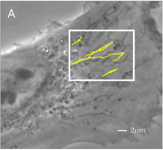
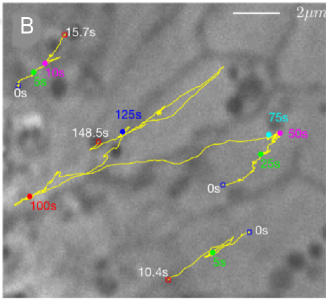
Figure 1: Cargoes movement along microtubules visualized in a living RPE cell (panel A). Panel B shows an enlargement of the boxed region in A. Trajectories (yellow) consists of long flights in one direction and multiple turnings. Numbers indicate the time progress. The longest trajectory ($148.5$ s) in the panel B consists of $900$ flights (see Sec. V for the description of the segmentation procedure).

I Introduction

Intracellular transport of cargoes along microtubules is a classical example of active transport Valle ; Bressloff . It is critical to cellular function and it is a challenging statistical problem from the viewpoint of active matter physics Loverdo ; Wang ; Trong ; Brangwynne ; Tabei . In-vitro experiments show that the distance travelled by cargoes substantially increases when the cargoes are transported by multiple motor proteins Vershinin . Various models have been developed that aim to explain how motors achieve long range transport along microtubules Lipowsky ; Berger11 ; Berger12 ; Bressloff1 ; Julicher ; Kolomeisky ; WelteGross98 ; MullerKlumppLipowsky ; Leidel ; Hancock ; Harrison ; Ajay .

Recently, it has been discovered that active cargo transport in-vivo self-organizes into Lévy walks Granick . Lévy walks describe a wide spectrum of biological processes, such as T-cells migrating in brain tissue, collective behaviour of swarming bacteria and animals optimizing their search for sparse food Zaburdaev . Endosomal Lévy dynamics involves long flights in one direction due to the active movement along microtubules driven by multiple motors. When all active motors disengage, the cargo complexes detach from the microtubule and reattach to a new microtubule heading in another direction Granick . The travel distances have power-law distributions with diverging variances MetzlerKlafter ; Barkai ; HF ; Sokolov ; Zaburdaev that determine the anomalously long flights of cargo complexes. In Ref. Granick the authors proposed the concept of memoryless self-reinforced directionality to demonstrate the emergence of Lévy walks.

However, the unanswered question remains: what is the precise mesoscopic kinetic mechanism of anomalous directional persistence? To answer this question, we performed in vivo experiments recording thousands of trajectories of intracellular lipid bound vesicles in live retinal pigment epithelium (RPE) cells and human bone osteosarcoma epithelial (U2OS) cells. We found similar results for both cell lines. Therefore, we report only results for RPE cells since a microscope with higher resolution was used to image them (see Section V for experimental details). In Fig. 1, we illustrate Lévy-like trajectories of vesicles inside RPE cells which consist of long persistent runs in one direction separated by rapid jiggling events when vesicles change direction.

In this paper we reveal a new mechanism for anomalous directional persistence of cargoes in human cells: the phenomenon of cumulative inertia. Experimentally we found the longer a cargo moves along a microtubule, the less likely it will detach from it. To our knowledge our data provides the first direct measurement of the mesoscopic detachment rate as a decreasing function of the running time. We found that this time follows a heavy tailed Pareto distribution which leads to a Lévy walk-like movement of cargoes. Since the observed detachment probability depends on how long the cargo has been moving, this active transport involves memory and it exhibits a typical non-Markovian behaviour. Note that we are dealing with the memory which is not physically or chemically stored or retrieved and therefore energetically costs the cells nothing.

II Empirical survival probability, mesoscopic detachment rate and mean residual time

One of our aims is to measure important statistical characteristics of cargo transport: the empirical survival probability of cargoes on the microtubule, the empirical mesoscopic detachment rate and the mean residual time.

The empirical survival probability defines the probability that the cargo have not detached from the microtubule (survived on the microtubule) beyond a specified time Aalen . It is a common tool in many areas such as Engineering and Medicine to measure the time-to-failure of machine parts or the fraction of patients living for a certain amount of time after treatment Aalen . The survival probability was estimated by using the non-parametric Kaplan-Meier estimator Aalen . We found a good agreement between the empirical survival probability $\Psi$ and the heavy tailed Pareto distribution:

$$\Psi(\tau)=(1+\tau/\tau_{0})^{-\alpha},$$ (1)

with the anomalous exponent $\alpha=1.6\pm 0.17$ and $\tau_{0}=0.17\pm 0.1$ s up to $1-2$ seconds (Fig. 2). The empirical mesoscopic detachment rate is also found to be a decreasing function of the flight time $\tau$ (inset Fig. 2). This means that the longer a cargo remains on a microtubule, the less likely it will detach from it (the phenomenon of cumulative inertia). Surprisingly, although having very different origin, similar effect of cumulative inertia is well studied and got revived interest in social and behavioural sciences Morrison ; FS .

Figure 2: The experimentally determined survival function $\Psi(\tau)$ (dots) as a function of time $\tau$ decays as a power law on intermediate time scales with an anomalous exponent $\alpha=1.6\pm 0.17$ and a time scale parameter $\tau_{0}=0.17\pm 0.1$ s. The errors were calculated with the Greenwood formula for the non-parametric Kaplan-Meier estimator Aalen . The red dashed curve is a power law fit Eq. (1) with the same $\alpha$ and $\tau_{0}$. The orange solid curve is the survival function obtained in numerical simulations of the Klumpp-Lipowsky model of the cargo dynamics with $6$ kinesin and $6$ dynein motors. Details of simulations are given in the section VI. Inset: the corresponding empirical mesoscopic detachment rate function $\gamma(\tau)$ (dots) as a function of time is inversely proportional to $\tau$, Eq. (2), on intermediate time scales (red dashed curve) with the same $\alpha$ and $\tau_{0}$ as in the main figure. The orange solid curve is the rate function obtained in numerical simulations.

The empirical mesoscopic detachment rate has a good fit with the rate inversely proportional to the flight time $\tau$:

$$\gamma(\tau)=\alpha/(\tau+\tau_{0}),$$ (2)

with the same anomalous exponent $\alpha=1.6\pm 0.17$ and $\tau_{0}=0.17\pm 0.1$ s. Note the relationship between $\Psi(\tau)$ and $\gamma(\tau)$: $\Psi(\tau)=\exp\left(-\int_{0}^{\tau}\gamma(t)dt\right)$. The time dependent detachment rate $\gamma(\tau)$ has the following meaning: the product $\gamma(\tau)\Delta\tau$ defines the conditional probability of cargo detachment in the interval $(\tau,\tau+\Delta\tau)$ given that it has moved along the microtubule in the time interval $(0,\tau)$. For memoryless cargoes this rate will be constant and will not depend on how long the cargo has moved before. It is well-known that the empirical rate is notoriously difficult to estimate Aalen , since it contains the derivative of the empirical survival function. Therefore, the empirical survival probability (which is an integral quantity) has a smoother behaviour compared to the empirical mesoscopic detachment rate function (Fig. 2).

The value of experimental exponent $\alpha=1.6\pm 0.17$ falls in the interval $1<\alpha<2$. This is an extraordinary finding since it shows that the survival function has a finite mean, $\left<T\right>=\int_{0}^{\infty}\tau\Psi(\tau)d\tau$, but divergent second moment Zaburdaev . Specifically the lack of the second moment leads to the emergence of the Lévy walk-like trajectories of vesicles (Fig. 1). Such trajectories exhibit sub-ballistic super-diffusive behaviour. We also obtain a good power law fit with the anomalous exponent ($\alpha\simeq 1.5\pm 0.17$) for the probability density of flight lengths (Fig. 3) which confirms the Lévy walk nature of the vesicles motion. The velocity $v$ of each flight was assumed to be constant. The probability density of flight length is obtained from the survival function as:

$$f(L)=-\Psi^{\prime}\left(L/v\right)/v,$$ (3)

where $\Psi^{\prime}(z)=d\Psi(z)/dz$. In Fig. 3 the distribution of flight velocities is also shown.

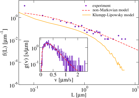
Figure 3: Main panel: The experimental flight length probability density $f(L)$ (blue dots) fitted with Eq. (3) (red dashed curve) with $\alpha=1.5\pm 0.17$, $\tau_{0}=0.33\pm 0.1$ s and the average velocity of the cargo $v=0.8$ $\mu$m/s. The flight length distribution obtained in numerical simulations of the cargo dynamics using the Klumpp-Lipowsky model with $6$ dynein and $6$ kinesin motors (orange solid curve) decays exponentially for $L>1$ $\mu$m. Parameters of the simulations are given in the section VI. The inset shows the distribution of experimental flight velocities $g(v)$ (blue solid curve) approximated with the Burr density (red dashed curve) with parameters $\tilde{\gamma}=0.57\pm 0.07$, $\tilde{c}=2.09\pm 0.09$, $\tilde{k}=2.00\pm 0.34$. The average velocity of the cargo is $v=0.8$ $\mu$m/s.

If the cargo has survived on the microtubule up to time $t$, how much longer is it expected to move (survive) along the microtubule? This time is called the mean residual time $\overline{T}(t)$ - another important quantitative measure of cumulative inertia. In vivo experiments we found that $\overline{T}(t)$ increases linearly in time $t$ already travelled, see Fig. 4. The longer the cargo remains on the microtubule, the larger the mean residual time, so the inertia is accumulated. This behaviour is drastically different to memoryless systems where $\overline{T}(t)$ is constant and does not depend on the prehistory. The data can be well explained by the conditional survival function for a random attachment time $T$, $\Psi_{c}(t,\tau)=\Pr\left\{T>t+\tau|T>t\right\}.$ In our case:

$$\Psi_{c}(t,\tau)=\frac{\Psi(t+\tau)}{\Psi(t)}=\left(\frac{\tau_{0}+t}{\tau_{0}+t+\tau}\right)^{\alpha},$$ (4)

is an increasing function of time $t$ already spent on the microtubule for a fixed $\tau$. The behaviour of $\Psi_{c}(t,\tau)$ is illustrated in the inset of Fig. 4. The mean residual time $\overline{T}(t)$ can be obtain as Morrison78 :

$$\overline{T}(t)=\int_{0}^{\infty}\Psi_{c}(t,\tau)d\tau=\frac{\tau_{0}+t}{\alpha-1}.$$ (5)

We found a good agreement between experimental mean residual time $\overline{T}(t)$ and Eq. (5) with $\tau_{0}=0.24\pm 0.1$ and the anomalous exponent $\alpha=1.8\pm 0.17$, Fig. 4. Notice that the values of anomalous exponents obtained by fitting experimental data $\alpha=1.6\pm 0.17$ in Fig. 2, $\alpha=1.5\pm 0.17$ in Fig. 3 and $\alpha=1.8\pm 0.17$ in Fig. 4 agree with each other within the error bars. This cumulative inertia with $1<\alpha<2$ explains the dramatic increases of the travelled distance that are typical for Lévy walk. Since this is a non-Markovian effect with memory, our explanation of anomalous long distance transport is completely different from the idea of memoryless self-reinforced directionality Granick when the probability $P(L)$ of traveling in some direction grows with the distance $L$ already travelled. This probability can be obtained in terms of the conditional survival function $\Psi_{c}(t,\tau)$ as $P(L)=\Psi_{c}(L/v,\tau)$.

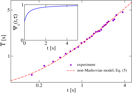
Figure 4: Main panel: The experimental mean residual time $\bar{T}$ of flights (blue dots) linearly increases (notice logarithmic scales on both the horizontal and vertical axes) with the time $t$ already travelled. The theoretical prediction Eq. (5) with parameters $\tau_{0}=0.24\pm 0.1$ s and $\alpha=1.8\pm 0.17$ (red dashed curve) is in good agreement with the experiment. Inset: Illustration of the increasing conditional survival function $\Psi_{c}(t,\tau)$ given by Eq. (4) with $\tau_{0}=0.2$ s, $\alpha=1.8$ and $\tau=0.1$ s.

III Microscopic mechanism for the emergence of the decreasing mesoscopic detachment rate

The question arises: what is the microscopic mechanism of the decreasing mesoscopic detachment rate $\gamma(\tau)$? A first insight could be obtained from a classical microscopic Klumpp-Lipowsky model Lipowsky . Note that the authors of Ref. Lipowsky did not consider this time dependent rate. Instead, they found a constant effective unbinding rate.

Consider a cargo which is pulled by multiple motors. We assume that initially the cargo attaches to the microtubule with a single motor. As the cargo moves along the microtubule, the number of engaged motors $N(t)$ varies from $1$ to $\bar{N}$. Motors attach to the microtubule and detach from it with effective microscopic rates $\pi_{n}$ and $\epsilon_{n}$ ($n$ is the number of engaged motors). We define the random detachment time $T$ as the time when all active motors together with the cargo detach from the microtubule. In other words we have a random walk in the space of the number of engaged motors. In order to obtain the effective detachment rate $\gamma(\tau)$, one can define the survival function $\Psi(\tau)$ of the cargo to remain on the microtubule as the probability $\Psi(\tau)=\text{Pr}\{T>\tau\}=1-\text{Pr}\{N(\tau)=0|N(0)=1\}$ Lipowsky . The effective detachment rate is defined as Cox :

$$\gamma(\tau)=-\Psi^{\prime}(\tau)/\Psi(\tau).$$ (6)

The function $\Psi(\tau)$ can be written in terms of the probability distribution of the first passage time $T$ from the cargo state with $1$ engaged motor at time $0$ to the cargo state with zero engaged motors:

$$F(\tau)=\Pr\left\{T<\tau\right\}$$ (7)

as

$$\Psi(\tau)=1-F(\tau).$$ (8)

To find the distribution function $F(\tau)$ one can introduce the transition probability Lipowsky

$$P_{n,0}(\tau)=\Pr\left\{N(\tau)=0|N(0)=n\right\}.$$ (9)

Define $F(\tau)$ as

$$F(\tau)=P_{1,0}(\tau),$$ (10)

where $P_{1,0}(\tau)$ is the transition probability from the cargo state with $1$ engaged motor to the state with zero engaged motors. $P_{n,0}(\tau)$ obey the system of the backward Kolmogorov equations Cox :

$$\frac{dP_{n,0}(t)}{dt}=-\left(\varepsilon_{n}+\pi_{n}\right)P_{n,0}(t)+\varepsilon_{n}P_{n-1,0}(t)+\pi_{n}P_{n+1,0}(t)$$ (11)

with the initial conditions $P_{n,0}(0)=0$ for $2\leq n\leq\bar{N},$ $P_{0,0}(t)=1$ ($n=0$ is the absorbing state). Here $\varepsilon_{n}$ and $\pi_{n}$ are the unbinding and binding rates. One can solve these equations and find the transition probability $P_{1,0}(\tau)$. It follows from Eqs. (6) and (8) that the effective detachment rate is

$$\gamma(\tau)=\frac{P^{\prime}_{1,0}(\tau)}{1-P_{1,0}(\tau)}.$$ (12)

This mesoscopic detachment rate is essentially different from the effective constant unbinding rate obtained within the Klumpp-Lipowsky model in Ref. Lipowsky from equilibrium conditions. It is time-dependent and decreasing function of $\tau$. Our purpose is to show that the rate $\gamma(\tau)$ is a decreasing function of the running time $\tau$. It means that the longer a cargo moves along the microtubule, the smaller is the probability that it will detach and switch the direction in the next time interval (a cumulative inertia effect). Numerical modelling confirms that $\gamma$ is a decreasing function of $\tau$ on a certain time scale (see the orange solid curve in the inset of Fig. 2).

In vitro experimental data indicates that adding just one extra motor increases cargo run lengths by at least one order of magnitude compared to the distance traveled by a single motor Vershinin . To understand intuitively the reason why $\gamma(\tau)$ decreases with the flight time $\tau$, consider the first event of attachment of cargo complex with one motor. Initially the rate $\gamma(0)=\epsilon_{1}$. Note that this defines the microscopic time scale $1/\epsilon_{1}$. In turn, the mesoscopic time scale is given by $\left<T\right>=\int_{0}^{\infty}\tau\Psi(\tau)d\tau$, $\left<T\right>\gg 1/\epsilon_{1}$. If the second motor attaches before the first motor detaches, the load is shared between two motors and the detachment rate $\epsilon_{2}$ decreases, $\epsilon_{2}<\epsilon_{1}$. As a result of this stochastic dynamics, the number of participating motors increases and therefore the detachment probability of the cargo decreases with the flight time. Cumulative inertia occurs due to multiple attachment and reattachment of motors before the cargo finally detaches from the microtubule. This leads to a dramatic increase of the travelled distance due to the directional persistence Vershinin .

We consider the cargo pulled by two motors $\bar{N}=2$ and show how the essential improvement of travel distance occurs. The backward Kolmogorov equations (11) take the form:

$$\frac{dP_{2,0}(t)}{dt} = -\varepsilon_{2}P_{2,0}(t)+\varepsilon_{2}P_{1,0}(t),$$ (13)

$$\frac{dP_{1,0}(t)}{dt} = -\left(\pi_{1}+\varepsilon_{1}\right)P_{1,0}(t)+\pi_{1}P_{2,0}(t)+\varepsilon_{1}$$ (14)

since $\pi_{2}=0.$ Solving above equations with the initial conditions $P_{1,0}(0)=P_{2,0}(0)=0,$ we find the cargo survival function $\Psi(t)=1-P_{1,0}(t):$

$$\Psi(t)=p_{1}e^{-k_{1}t}+p_{2}e^{-k_{2}t},$$ (15)

where

$$p_{1}=\frac{\varepsilon_{1}}{k_{2}}\left(\frac{k_{2}-\varepsilon_{1}}{k_{2}-k_{1}}\right),\,\,\,\,\,\,p_{2}=\frac{\varepsilon_{1}}{k_{1}}\left(\frac{\varepsilon_{1}-k_{1}}{k_{2}-k_{1}}\right).$$ (16)

Here two real eigenvalues $k_{1}$ and $k_{2}$ ($k_{1}<k_{2}$) are the solution of the quadratic equation

$$k^{2}-(\pi_{1}+\varepsilon_{1}+\varepsilon_{2})k+\varepsilon_{1}\varepsilon_{2}=0.$$ (17)

Since

$$p_{1}+p_{2}=1$$ (18)

the survival function (15) has an interesting probabilistic interpretation if $\varepsilon_{2}-k_{1}>0$ and $k_{2}-\varepsilon_{2}>0$ (both $p_{1}$ and $p_{2}$ are positive). The cargo movement can be interpreted as one that involves a mixed population of two motors with different properties. The first motor has a probability $p_{1}$, to be engaged and it has the exponential density of dwelling times with a rate $k_{1}$. $p_{2}$ is the probability of engagement for the second type of motor with an effective detachment rate $k_{2}.$ In this case the rate $\gamma(\tau)$ defined by (12) is always a decreasing function of running time $\tau$:

$$\gamma(\tau)=\frac{p_{1}k_{1}e^{-k_{1}\tau}+p_{2}k_{2}e^{-k_{2}\tau}}{p_{1}e^{-k_{1}\tau}+p_{2}e^{-k_{2}\tau}}.$$ (19)

This explains the dramatic increase of run length of a cargo with two motors and non-Markovian nature of cargo movement. The detachment rate $\gamma(\tau)$ takes the maximum value at $\tau=0$:

$$\gamma(0)=p_{1}k_{1}+p_{2}k_{2}=\varepsilon_{1}.$$ (20)

In the long time limit, the detachment rate $\gamma(\tau)$ tends to the constant value $k_{1}$ such that $k_{1}<\varepsilon_{1}.$ This explains the dramatic increase of run length of a cargo with two motors and the non-Markovian nature of cargo movement. Our numerical results support this idea and show a decreasing detachment rate $\gamma$ (inset Fig. 2). Note that the empirical power-law survival function can be approximated with the survival function in the form of the linear combination of exponents corresponding to the Klumpp-Lipowsky model (Fig. 2).

The survival function Eq. (15) has an interesting biological interpretation. The cargo movement can be viewed as one that involves a mixed population of two motors with different properties. If we extend this idea to a heterogeneous population of motors for which the rates $k$ are gamma distributed with the probability density function $f(k)=\tau_{0}k^{\alpha-1}e^{-\tau_{0}k}/\Gamma(\alpha)$, the effective survival function takes the form $\Psi(\tau)=\int_{0}^{\infty}e^{-k\tau}f(k)dk=(1+\tau/\tau_{0})^{-\alpha}$ consistent with Eq. (1).

IV Non-Markovian dynamics of cargo: super-diffusion

Our next aim is to provide a theoretical link between the empirical mesoscopic detachment rate and the experimental Lévy walk-like trajectories. The mesoscopic detachment rate Eq. (2) with the anomalous exponent $1<\alpha<2$ applied in Eq. (21) allows us to explain the emergence of a Lévy walk as a result of anomalous cumulative inertia phenomena. We obtain the mean squared displacement (msd) which exhibits sub-ballistic super-diffusive behaviour $\left<\mathbf{x}^{2}(t)\right>\sim t^{3-\alpha}$. For Lévy walk with $1<\alpha<2$ the ensemble and time averaged msds differ only by a factor of $1/(\alpha-1)$ ZK ; FB ; MJCB .

Define the probability density function $\xi(t,\mathbf{x},\varphi,\tau)$ which gives the probability to find a cargo at point $\mathbf{x}=(x,y)$ at time $t$ that moves with the velocity $v$ in the direction $\bm{\mathbf{\theta}}=(\cos\varphi,\sin\varphi)$ and having started the move a time $\tau$ ago. Here $\varphi$ is the angle between the direction of movement $\bm{\mathbf{\theta}}$ and the $x$ axis. We assume that as long as the cargo detaches from the microtubule it reattaches to another microtubule and thereby changes the direction of movement. The governing equation for $\xi(t,\mathbf{x},\varphi,\tau)$ takes the form Alt

$$\frac{\partial\xi}{\partial t}+v\bm{\mathbf{\theta}}\bm{\mathbf{\cdot\nabla}}\xi+\frac{\partial\xi}{\partial\tau}=-\gamma(\tau)\xi,$$ (21)

with the boundary condition

$$\xi(t,\mathbf{x},\varphi,0)=\int_{0}^{t}\gamma(\tau)\int_{-\pi}^{\pi}R\left(\varphi-\varphi^{\prime}\right)\xi(t,\mathbf{x},\varphi^{\prime},\tau)d\mathbf{\varphi}^{\prime}d\tau,$$ (22)

where $R\left(\varphi-\varphi^{\prime}\right)$ is the probability density of the re-orientation from $\varphi^{\prime}$ to $\varphi$ such that $\int_{-\pi}^{\pi}R\left(u\right)du=1.$ In Ref. Granick the flights were statistically isotropic with $R\left(u\right)=1/{2\pi}$. In our experiments, we observe quasi one-dimensional trajectories (Fig. 1) for which the angle takes only two values Fedotov16 .

The aim of this section is to obtain the non-Markovian master equation for the probability density:

$$p(t,\mathbf{x},\varphi)=\int_{0}^{t}\xi(t,\mathbf{x},\varphi,\tau)d\tau,$$ (23)

where the $\xi$ is the structural density. We assume that at the initial time $t=0$ cargo has a zero running time

$$\xi(t,\mathbf{x},\varphi,0)=p^{0}(t,\mathbf{x},\varphi)\delta(\tau),$$ (24)

where $p^{0}(t,\mathbf{x},\varphi)$ is the initial density. The density $p(t,\mathbf{x},\varphi)$ can be found by differentiating (23) with respect to time $t$:

$$\frac{\partial p}{\partial t}+v\bm{\mathbf{\theta\cdot\nabla}}p=-i(t,\mathbf{x},\varphi)+j(t,\mathbf{x},\varphi),$$ (25)

where $v$ is the cargo velocity, $\bm{\mathbf{\theta}}=(\cos(\varphi),\sin(\varphi))$ is the direction of cargo’s movement. The switching terms are:

$$i(t,\mathbf{x},\varphi)=\int_{0}^{t}\gamma(\tau)\xi(t,\mathbf{x},\varphi,\tau)d\tau,$$ (26)

$$j(t,\mathbf{x},\varphi)=\xi(t,\mathbf{x},\varphi,0)=$$ (27)

$$=\int_{0}^{t}\int_{-\pi}^{\pi}R\left(\varphi-\varphi^{\prime}\right)\gamma(\tau)\xi(t,\mathbf{x},\varphi^{\prime},\tau)d\varphi^{\prime}d\tau.$$

By using the method of characteristics we find for $\tau<t$:

$$\xi(t,\mathbf{x},\varphi,\tau)=\xi(t-\tau,\mathbf{x-}v\bm{\mathbf{\theta}}\tau,\varphi,0)e^{-\int_{0}^{\tau}\gamma(s)ds}.$$ (28)

The exponential factor in the above formula is the survival function:

$$\Psi(t)=e^{-\int_{0}^{t}\gamma(s)ds}.$$ (29)

To obtain $i(t,\mathbf{x},\varphi),$ we use the Fourier-Laplace transform:

$$\hat{\tilde{i}}(s,\mathbf{k},\varphi)=\int_{\mathbb{R}^{2}}\int_{0}^{\infty}i(t,\mathbf{x},\varphi)e^{i\bm{\mathbf{k\cdot x}}-st}dtd\mathbf{x},$$ (30)

$$\hat{\tilde{p}}(s,\mathbf{k},\varphi)=\int_{\mathbb{R}^{2}}\int_{0}^{\infty}p(t,\mathbf{x},\varphi)e^{i\bm{\mathbf{k\cdot x}}-st}dtd\mathbf{x}.$$ (31)

We find:

$$\hat{\tilde{i}}(s,\mathbf{k},\varphi)=\tilde{K}(s-iv\bm{\mathbf{k\cdot\theta}})\hat{\tilde{p}}(s,\mathbf{k},\varphi),$$ (32)

where $\tilde{K}(s)=\tilde{\psi}(s)/\tilde{\Psi}(s).$ Finally we obtain the expressions for the switching terms:

$$i(t,\mathbf{x},\varphi)=\int_{0}^{t}K(s)p(t-s,\bm{\mathbf{x}}-v\bm{\mathbf{\theta}}s,\varphi)ds,$$ (33)

$$j(t,\mathbf{x},\varphi)=\int_{-\pi}^{\pi}R\left(\varphi-\varphi^{\prime}\right)i(t,\mathbf{x},\varphi^{\prime})d\varphi^{\prime}.$$ (34)

The main advantage of the present derivation is that it can be easily extended for the nonlinear case.

Super-diffusive equations can be obtained for the case when the detachment rate $\gamma(\tau)$ can be approximated by the following rate

$$\gamma(\tau)=\frac{\alpha}{\tau_{0}+\tau},\ 1<\alpha<2.$$ (35)

The rate (35) leads to a power law (Pareto) survival function:

$$\Psi(\tau)=\left[\frac{\tau_{0}}{\tau_{0}+\tau}\right]^{\alpha}$$ (36)

and corresponding running time PDF:

$$\psi(\tau)=\frac{\alpha\tau_{0}^{\alpha}}{(\tau_{0}+\tau)^{1+\alpha}}.$$ (37)

The Laplace transform can be written in terms of the incomplete gamma function $\Gamma(a,b)=\int_{b}^{\infty}t^{a-1}e^{-t}dt$ as:

$$\tilde{\psi}(s)=\alpha\left(\tau_{0}s\right)^{\alpha}e^{\tau_{0}s}\Gamma\left(-\alpha,\tau_{0}s\right).$$ (38)

In the long-time limit as $s\rightarrow 0$, we have

$$\Gamma\left(-\alpha,\tau_{0}s\right)=-\frac{\Gamma(1-\alpha)}{\alpha}+\left(\tau_{0}s\right)^{-\alpha}\alpha^{-1}+\frac{\left(\tau_{0}s\right)^{1-\alpha}}{1-\alpha}+...$$ (39)

For $1<\alpha<2,$ using $\Gamma\left(-\alpha\right)=\frac{\Gamma(2-\alpha)}{\alpha\left(\alpha-1\right)}$ we obtain:

$$\tilde{\psi}(s)\simeq 1-\frac{\tau_{0}s}{\alpha-1}+\frac{\Gamma(2-\alpha)\left(\tau_{0}s\right)^{\alpha}}{\left(\alpha-1\right)},\qquad s\rightarrow 0$$ (40)

or

$$\tilde{\psi}\left(s\right)\simeq 1-{\overline{T}}s+\Gamma(2-\alpha)\tau_{0}^{\alpha-1}{\overline{T}}s^{\alpha},$$ (41)

where ${\overline{T}}=\tau_{0}\left(\alpha-1\right)^{-1}$ is the mean value of the random running time $T.$ Then

$$\tilde{K}(s)=\frac{s\tilde{\psi}(s)}{1-\tilde{\psi}(s)}\simeq\frac{1}{{\overline{T}}}\left(1+\Gamma(2-\alpha)\left(\tau_{0}s\right)^{\alpha-1}\right)$$

as $s\rightarrow 0.$ Using (32) we write the Fourier-Laplace transform of $i(t,\mathbf{x},\varphi)$ as:

$$\hat{\tilde{i}}=\frac{1}{{\overline{T}}}\left(1+\Gamma(2-\alpha)\tau_{0}^{\alpha-1}\left(s-iv\bm{\mathbf{k\cdot\theta}}\right)^{\alpha-1}\right)\hat{\tilde{p}}.$$ (42)

The switching term $i(t,\mathbf{x},\varphi)$ can be written as SK :

$$i=\frac{1}{{\overline{T}}}\left[1+\Gamma(2-\alpha)\tau_{0}^{\alpha-1}\left(\frac{\partial}{\partial t}-v\bm{\mathbf{\theta\cdot\nabla}}\right)^{\alpha-1}\right]p.$$ (43)

where the fractional material derivative $\left(\frac{\partial}{\partial t}-v\bm{\mathbf{\theta\cdot\nabla}}\right)^{\alpha-1}$ of order $\alpha-1$ is defined by their Fourier-Laplace transforms

$$\mathcal{LF}\left\{\left(\frac{\partial}{\partial t}-v\bm{\mathbf{\theta\cdot\nabla}}\right)^{\alpha-1}p\right\}=(s-iv\bm{\mathbf{k\cdot\theta}})^{\alpha-1}\tilde{p}(s,\mathbf{k},\varphi).$$ (44)

Taking the Laplace transform of Eq. (25), substituting the Laplace transform of Eq. (43) into it (using Eq. (34)) and Eq. (42), we solve the equation for $\tilde{p}$. Then, differentiating $\tilde{p}$ twice and taking the inverse Laplace transform, we find the mean squared displacement $\left<\mathbf{x}^{2}(t)\right>$. For the isotropic case with the uniform angle distribution $R\left(u\right)=1/{2\pi}$ (Granick data Granick ) or quasi one-dimensional distribution (our data) the mean squared displacement exhibits sub-ballistic super-diffusive behaviour

$$\left<\mathbf{x}^{2}(t)\right>\sim t^{3-\alpha},\qquad 1<\alpha<2.$$ (45)

In Fig. 5 we show the time averaged mean squared displacement calculated for single experimental trajectories (corrected for the drift) which was also averaged over many trajectories. A clear power-law behaviour with the exponent $1.51\pm 0.17$ is found which is consistent with the Lévy walk behaviour and with the behaviour of the detachment rate and survival functions.

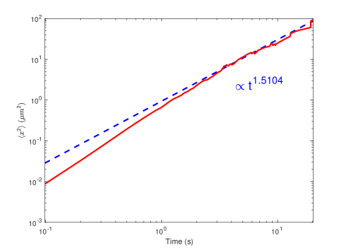
Figure 5: Anomalous behaviour of the time averaged mean squared displacement for experimental trajectories in RPE cell (corrected for the drift and averaged over many trajectories). The dashed curve represents the power law function with the exponent $1.5\pm 0.17$.

V Experimental Methods and Analysis of Trajectories

Intracellular vesicles of U2OS (human bone osteosarcome epithelial) and RPE (retinal pigment epithelial) cells were imaged using phase contrast microscopy and tracked with Polyparticle Tracker software rogers2007 . The cells were grown in DMEM (Sigma Life Science) and 10% FBS (HyClone) and incubated for 48 hrs at 37^∘C in 8% CO₂ on 35 mm glass-bottomed Ibidi dishes. Before imaging, the cells were moved to a live-imaging media. The live-cell imaging was done using an inverted Olympus IX71 with an Olympus 100$\times$/1.35 oil PH3 objective and 1.6$\times$ zoom. A QuantEM 512SC CCD Camera and Cool LED pE-100 light source was used for the continuous imaging of U2OS cells and a CoolSNAP HQ2 was used for the RPE cells. The video was taken with 30 ms or 98.5 ms exposure times while the cells were kept at 37^∘ in atmospheric CO₂ levels.

After tracking each vesicle’s path, only those with maximum displacements greater than 1 $\mu$m were chosen. Our aim was to filter those vesicles that are involved in active transport along microtubules. For this reason, we used the time averaged mean square displacements (MSDs) for single vesicle trajectories:

$$\langle\mathbf{x}^{2}(m\delta t)\rangle=\frac{1}{N-m}\sum_{i=1}^{N-m}(\mathbf{x}(t_{i}+m\delta t)-\mathbf{x}(t_{i}))^{2},$$ (46)

where $\mathbf{x}=(x,y)$ is the vesicle coordinate and the video contains $N$ snapshots at increments of $\delta t$. The total time of a data set is then $T=(N-1)\delta t$ and $m=1,2,...,N-1$. Lag-times were defined as the set of possible $m\delta t$ within the data set. Trajectories with mean square displacements (MSDs) close to $t^{2}$ (active transport) were analysed Arcizet . The lower limit for the MSD was balanced between sufficient statistics to produce good fits and its proximity to $t^{2}$ proportionality.

To measure the turning times of the vesicles, an angular threshold method was used in conjunction with a distance threshold. In a set of $N$ points, there will be $N-2$ angles characterizing the direction of the path and for three arbitrary data points, $i$, $i+1$ and $i+2$, the angle deviation of the path was calculated by Harrison :

$$\theta_{i+1}=\arccos\left(\frac{\mathbf{x}_{i\rightarrow(i+1)}\cdot\mathbf{x}_{(i+1)\rightarrow(i+2)}}{|\mathbf{x}_{i\rightarrow(i+1)}||\mathbf{x}_{(i+1)\rightarrow(i+2)}|}\right).$$ (47)

If $\theta_{i+1}>\theta_{max}$, the path was deemed to have changed direction. Additionally, if the tracked vesicle had not moved greater than 10% of the length of a pixel, during the turn, the path was deemed to not have changed direction. This threshold was to ensure that stationary or completely detached vesicles, that move diffusively, do not add false runs to the statistics. In order to ensure results were not dependent on the arbitrary value of $\theta_{\text{max}}$, a set of threshold angles were tested ranging from 5^∘ to 90^∘ in 5^∘ increments. We found $\theta_{\text{max}}=45^{\circ}$ to be optimal. With such an angular threshold, we have a good quality of the trajectory segmentation as shown in Fig. 6.

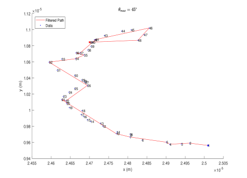
Figure 6: The Cartesian position of a tracked particle path segmented using $\theta_{\text{max}}=45^{\circ}$. Blue dots with frame numbers mark the path. The red line indicates the new segmented path. The blue star marks the start position and the red star marks the end position.

VI Numerical modelling

In experimental trajectories we found retrograde (towards the cell centre) and anterograde (away from the cell centre) movement which suggest that vesicles are driven by both kinesins and dyneins. However, we observe no long pauses between retrograde and anterograde movement (Fig. $1$) and conclude that it is unlikely that kinesins and dyneins were engaged in a tug-of-war WelteGross98 ; MullerKlumppLipowsky . Instead, changes of the direction could be triggered by some regulatory mechanism which remains poorly understood Hancock ; Leidel .

To model the multi-motor cargo transport we consider two groups of kinesin and dynein motors. Only kinesins or dyneins are engaged in cargo movement at any time. There are some indications (although still debated in the literature) that motors are loaded on the cargo in pairs Johnston . We suppose that there is an equal number of kinesins and dyneins. The groups can change after the number of engaged motors reaches zero and the cargo detaches from the microtubules. We assume that initially the cargo attaches to the microtubule with a single kinesin or dynein motor and moves along it pulled by $N(t)$ motors of one polarity. The number of engaged motors $N(t)$ varies from $1$ to $\bar{N}$. The motors detach and reattach with rates $\varepsilon_{n}$ and $\pi_{n}$. It is assumed that all the motors equally share the external load.

The number of kinesins and dyneins decreases and increases with the rates $\varepsilon_{n}$ and $\pi_{n}$ give by KunwarMogilner :

$$\varepsilon_{n}=n\varepsilon e^{\frac{F_{v}}{nF_{d}}},\;\;\;\pi_{n}=\pi(\bar{N}-n),$$ (48)

where $F_{v}$ is the force acting on the cargo which depends on its velocity $v$, $F_{d}$ is the corresponding detachment force for kinesin or dynein, $\pi$ is the binding constant for a single kinesin or dynein motor and $\varepsilon$ is their zero-load unbinding rate. The values of $\pi$, $\varepsilon$ and $\bar{N}$ were adjusted to match the experimental data.

The cargo pulled by $n$ motors has the velocity

$$v(F_{v})=v\left(1-\frac{F_{v}}{nF_{s}}\right),$$ (49)

where $F_{s}$ is the motor stall force and $v$ is the load-free velocity. The force $F_{v}$ which is acting on the cargo of radius $r$ due to viscous resistance also depend on the velocity of the cargo $F_{v}=6\pi\eta rv$. Substituting this into Eq. (49) and solving for the velocity, the consistent expression for the velocity is KunwarMogilner :

$$v(F_{v})=\frac{v}{1+(6\pi\eta rv)/(nF_{s})}.$$ (50)

In our experiment, the typical radius of the lipid bound vesicles was $0.5$ $\mu$m. The cytoplasm is estimated to be $1000$ times more viscous than the buffer Luby-Phelps , $\eta=0.89$ Pa s. Below we give the set of parameters used in simulations shown in Fig. $2$ in the main text. We have used parameters for kinesins and dyneins from Ref. Kunwar . For kinesins: $v=1$ $\mu$m/s, $\pi=1$ s^-1, $\varepsilon=2$ s^-1, $F_{d}=4$ pN, $F_{s}=5$ pN For dyneins: $v=1$ $\mu$m/s, $\pi=1$ s^-1, $\varepsilon=3$ s^-1, $F_{d}=0.87$ pN, $F_{s}=1.25$ pN.

VII Discussion and Conclusion

In summary, we studied experimentally the non-Markovian anomalous multi-motor intracellular transport of cargoes inside cells. To our knowledge, we for the first time directly measured the mesoscopic detachment rate of cargoes from microtubules and demonstrated that the origin of the anomalous non-Markovian behavior is the cumulative inertia phenomenon. We provided evidence for this phenomenon in both bone and retina epithelial cells, but it is expected to occur in all cell types that use dyneins and kinesins to transport cargoes along microtubules. We proposed a mesoscopic model which explains the emergence of memory and non-Markovian behaviour in the intracellular cargo transport on a mesoscopic scale. We also demonstrated how this non-Markovian behaviour emerged from Markovian memoryless dynamics of multiple motors on a microscopic scale. At the same time we note that the microscopic model is inconvenient since it has multiple parameters which require difficult fine tuning. And more importantly, almost all parameters in the microscopic model are unknown in vivo. There is no experimental technique to measure them. On the contrary, our mesoscopic model is computationally cheap and has only two parameters which we measure directly in the experiment. We believe that our model provides a complementary description of the intracellular transport on a mesoscopic scale that is better able to model the experimentally observed memory effects.

The impact of our work on the field of intracellular transport will be three-fold: firstly, for the first time we experimentally show the non-Markovian nature of intracellular transport and memory effects on a mesoscopic scale. Secondly, our results settle the controversy in the field of intracellular transport (see the work of Granick and co-workers in Nature Materials 2015) about memory-less Markovian dynamics on a microscopic scale and non-Markovian behavior and memory effects on a mesoscopic scale. Thirdly, with our work we are shifting the paradigm of how the single-particle tracking experiments could be analysed by introducing several new mesoscopic statistical quantities, such as the mesoscopic detachment rate, the survival function and the mean residual time to remain on the microtubule. We believe that these quantities are better for a description of the long time properties of intracellular transport than the traditionally used mean squared displacements along single trajectories. What is important, is that we show that these quantities are experimentally measurable, can be predicted and can be modelled in a self-consistent manner (improving our confidence in the robustness of our analysis). Improved non-Markovian modelling will lead to more accurate quantitative analysis of the kinetics of a huge range of active transport in cellular physiology. Such transport impacts on a vast range of cellular processes and their diseased states e.g. motor neuron disease and cancer.

- (1) R. D. Vale, The Molecular Motor Toolbox for Intracellular Transport. Cell 112, 467-480 (2003).
- (2) P. C. Bressloff, Stochastic Processes in Cell Biology. (4 ed.) Springer, 2014.
- (3) C. Loverdo, O. Benichou, M. Moreau, and R. Voituriez, Enhanced reaction kinetics in biological cells. Nature Phys. 4, 134-137 (2008).
- (4) B. Wang, J. Kuo, and S. Granick, Bursts of active transport in living cells. Phys. Rev. Lett. 111, 208102 (2013).
- (5) P. K. Trong, J. Guck, and R. E. Goldstein, Coupling of active motion and advection shapes intracellular cargo transport. Phys. Rev. Lett. 109, 028104 (2012).
- (6) C. P. Brangwynne, G. H. Koenderink, F. C. MacKintosh and D. A. Weitz, Intracellular transport by active diffusion. Trends Cell Biol. 19, 423-427 (2009).
- (7) S. M. A. Tabei et al., Intracellular transport of insulin granules is a subordinated random walk. Proc. Natl Acad. Sci. USA 110, 4911-4916 (2013).
- (8) M. Vershinin, B. C. Carter, D. S. Razafsky, S. J. King, and S. P. Gross, Multiple-motor based transport and its regulation by Tau, Proceedings of the National Academy of Sciences, USA 104, 87-92. (2007).
- (9) S. Klumpp and R. Lipowsky, Cooperative cargo transport by several molecular motors, Proceedings of the National Academy of Sciences, USA 102, 17284-17289 (2005).
- (10) F. Berger, C. Keller, M. J. I. Müller, S. Klumpp, and R. Lipowsky, Co-operative transport of molecular motors. Biochem. Soc. Trans. 39, 1211-1215 (2011).
- (11) F. Berger, C. Keller, S. Klumpp, and R. Lipowsky, Distinct transport regimes for two elastically coupled molecular motors. Phys. Rev. Lett. 108, 208101 (2012).
- (12) P. C. Bressloff and J. M. Newby, Stochastic models of intracellular transport, Rev. Mod. Phys. 85, 135-196 (2013).
- (13) F. Jülicher, A. Ajdari, and J. Prost, Modeling molecular motors. Rev. Mod. Phys. 69, 1269-1281 (1997).
- (14) A. B. Kolomeisky and M. E. Fisher, Molecular motors: a theorist’s perspective. Annu. Rev. Phys. Chem. 58, 675-695 (2007).
- (15) M. A. Welte, S. P. Gross, M. Postner, S. M. Block, & E. F. Wieschaus, Developmental regulation of vesicle transport in Drosophila embryos: forces and kinetics, Cell 92, 547-557 (1998).
- (16) M. J. Müller, S. Klumpp, & R. Lipowsky, Tug‑of‑war as a cooperative mechanism for bidirectional cargo transport by molecular motors. Proc. Natl Acad. Sci. USA 105, 4609-4614 (2008).
- (17) C. Leidel, R. A. Longoria, F. M. Gutierrez, and G. T. Shubeita, Measuring Molecular Motor Forces In Vivo: Implications for Tug-of-War Models of Bidirectional Transport, Biophysical Journal 103, 492-500 (2012).
- (18) W. O. Hancock, Bidirectional cargo transport: moving beyond tug of war, Nature Reviews Molecular Cell Biology 15, 615-628 (2014).
- (19) A. W. Harrison, D. A. Kenwright, T. A. Waigh, P. G. Woodman, V. J. Allan, Modes of correlated angular motion in live cells across three distinct time scales, Phys. Biol. 10, 036002 (2013).
- (20) Q. Li, S. King, A. Gopinathan, and J. Xu, Quantitative determination of the probability of multiple-motor transport in bead-based assays, Biophysical Journal 110, 2720-2728 (2016).
- (21) D. G. Morrison and D. C. Schmittlein, Jobs, strikes, and wars: Probability models for duration. Organ. Behav. Hum. Perform. 25, 224-251 (1980).
- (22) S. Fedotov and H. Stage, Anomalous Metapopulation Dynamics on Scale-Free Networks. Phys. Rev. Lett. 118, 098301 (2017).
- (23) K. Chen, B. Wang and S. Granick, Memoryless self-reinforcing directionality in endosomal active transport within living cells, Nature Materials 14, 589-593 (2015).
- (24) V. Zaburdaev, S. Denisov, and J. Klafter, Lévy walks, Rev. Mod. Phys. 87, 483-530 (2015).
- (25) R. Metzler and J. Klafter, The restaurant at the end of the random walk: recent developments in the description of anomalous transport by fractional dynamics, J. Phys. A: Math. Gen. 37, R161-R208 (2004).
- (26) Barkai, E. Garini, Y. & Metzler, R. Strange kinetics of single molecules in living cells. Phys. Today 65, 29-35 (2012).
- (27) Höfling, F. & Franosch, T. Anomalous transport in the crowded world of biological cells. Rep. Prog. Phys. 76, 046602-046652 (2013).
- (28) Klafter, J. & Sokolov, I. M. First steps in random walks: from tools to applications., Oxford University Press, 2011.
- (29) S. S. Rogers, T. A. Waigh, X. Zhao, and J. R. Lu, Precise particle tracking against a complicated background: Polynomial fitting with Gaussian weight. Phys. Biol. 4, 220-227 (2007).
- (30) D. Arcizet, B. Meier, E. Sackmann, J. O. R’́adler, and Doris Heinrich, Temporal Analysis of Active and Passive Transport in Living Cells. Phys. Rev. Lett. 101, 248103 (2008).
- (31) O. Aalen, Ø. Borgan, H. Gjessing, Survival and event history analysis: a process point of view. (Springer, 2008).
- (32) D. G. Morrison, On linearly increasing mean residual lifetimes, J. Appl. Prob. 15, 617-620 (1978).
- (33) D. R. Cox, H. D. Miller. The Theory of Stochastic Processes (Methuen, London, 1965).
- (34) G. Zumofen and J. Klafter, Power spectra and random walks in intermittent chaotic systems. Phys. D 69, 436-446 (1993).
- (35) D. Froemberg and E. Barkai, Time-averaged Einstein relation and fluctuating diffusivities for the Lévy walk. Phys. Rev. E 87, 030104(R) (2013).
- (36) R. Metzler, J.-H. Jeon, A. G. Cherstvy and E. Barkai, Anomalous diffusion models and their properties: non-stationarity, non-ergodicity, and ageing at the centenary of single particle tracking. Phys. Chem. Chem. Phys. 16, 24128-24164 (2014).
- (37) W. Alt, Biased random walk models for chemotaxis and related diffusion approximations. J. Math. Biol. 9, 147-177 (1980).
- (38) S. Fedotov, Single integrodifferential wave equation for a Lévy walk. Phys. Rev. E. 93, 020101 (2016).
- (39) I. M. Sokolov and R. Metzler, Towards deterministic equations for Lévy walks: The fractional material derivative, Phys. Rev. E 67, 010101(R) (2003).
- (40) D. St. Johnston, Counting Motors by Force, Cell 135, 1000-1001 (2008).
- (41) A. Kunwar and A. Mogilner, Phys. Biol 7, 016012 (2010).
- (42) K. Luby-Phelps, Int. Rev. Cytol. 192, 189-221 (2000).
- (43) A. Kunwar et al., Mechanical stochastic tug-of-war models cannot explain bidirectional lipid-droplet transport. Proc. Natl Acad. Sci. USA 108, 18960-18965 (2011).