Core collapse with magnetic fields and rotation

Abstract

We study the effects of magnetic fields and rotation on the core collapse of a star of an initial mass of $M=20\,M_{\odot}$ using axisymmetric simulations coupling special relativistic magnetohydrodynamics, an approximately relativistic gravitational potential, and spectral neutrino transport. We compare models of the same core with different, artificially added profiles of rotation and magnetic field. A model with weak field and slow rotation does not produce an explosion, while stronger fields and fast rotation open the possibility of explosions. Whereas the neutrino luminosities of the exploding models are the same as or even less than those of the non-exploding model, magnetic fields locally in equipartition with the gas pressure provide a strong contribution to the shock revival and the acceleration of bipolar outflows. Among the amplification processes generating such strong fields, we find the magneto-rotational instability. However, our limited grid resolution allows us to find it only in limited regions of the model with the strongest pre-collapse field ($10^{11}\,\textrm{G}$) and fastest rotation.

1 Introduction

The evolution of stars with masses above $\gtrsim 8M_{\odot}$, depends on parameters such as the metallicity, the initial mass, the rotational profile, and the magnetic field of the star, for which nature offers a wide range of possibilities. Moreover, it also depends on processes such as convection and other (hydrodynamic) instabilities, mass loss, and mass transfer within binary systems, whose complex dynamics increase the spectrum of evolutionary paths [29]. The resulting diversity of conditions of stellar cores after the end of their hydrostatic evolution translates into very different scenarios for the evolution after core bounce. Besides the action of neutrino heating in combination with hydrodynamic instabilities, magnetic fields and rotation may contribute to revive the stalled shock wave and launch a core-collapse supernova (CCSN) explosion. Furthermore, shock revival may completely fail in a substantial fraction of all cores, leading finally to the formation of a black hole (BH) rather than a neutron star as in most other cases [1].

Supernova theory has accounted for this large diversity by, e.g., studying the standard neutrino-driven mechanism across a wide range of progenitor masses (for recent work, see e.g., [51, 65, 7, 44, 31, 61, 41]) as well as by considering alternative processes contributing to shock revival and explosion such as modifications of nuclear physics [19]. Rotation and magnetic fields are among the most important such alternatives. Similar to the simulations set within the standard scenario, magneto-rotational models have increased in complexity since the pioneering works of [30, 37, 5, 43]. Very likely, the foremost effect that the combined action of magnetic fields and rotation may bring is the exponential amplification of seed fields mediated by the magneto-rotational instability (MRI). The MRI is the most promising candidate among the different possibilities for field amplification. Other alternatives, e.g. amplification of the magnetic field due to the core compression, winding of the poloidal into toroidal field, or hydrodynamic instabilities (convection and the standing accretion shock instability, SASI), are less effective in producing dynamically relevant magnetic fields after core bounce [50]. The possibility that the MRI indeed was operative in the context of core collapse opened up in simplified, spherically symmetric models [2], in which large regions of the post-bounce core were identified as MRI unstable. That seminal work spurred various studies of axisymmetric collapse examining this result more closely and exploring the consequences of a strong field created by the MRI. Some of the earlier works had used very approximate equations of state (EOSs) and neglected neutrinos altogether [48, 47, 11, 56], others treated neutrinos in a simplified manner [3, 4, 38, 25, 64], while a few studies were performed with state-of-the-art neutrino transport [8, 15, 46].

These simulations commonly show the development of jets driven by the magnetic field and powered by the rotational energy of the core if the energy density of the magnetic field is locally similar to that of the velocity field. Although this possibility cannot be excluded in principle, the weak pre-collapse fields predicted by current stellar evolution modelling [21] make it exceedingly unlikely to reach such a configuration without the presence of efficient field amplification after bounce. Following the evolution of the MRI is technically very challenging because the length scales on which it grows fastest is directly proportional to the seed field strength. On the numerical grids commonly employed in core collapse models, these scales can only be resolved if the initial field is already very strong, in which case the need for additional MRI-mediated amplification is less pronounced. Consequently, such simulations cannot address the question whether the MRI is able to amplify a realistically weak pre-collapse field to dynamically relevant strength. Instead, [49, 36, 55, 54] performed local or semi-global three-dimensional simulations derived from the shearing-box models of accretion-disk theory [20] with a reduced amount of physics ingredients, but very high resolution. The results, in particular when combined with an analytical treatment of the MRI growth, indicate that the factor by which the MRI can amplify the seed field is limited by the development of secondary, parasitic instabilities of Kelvin-Helmholtz type [54]. More recently, growing computational power has allowed for an increased resolution in global models specifically aimed at studying the MRI, albeit with greatly simplified physics and only in axisymmetry [58, 57] or with a very restricted three-dimensional geometry [35]. Hence, the question of MRI-driven field amplification remains open.

Aside from leading to a wrong hydrodynamic turbulent cascade and restricting the development of important non-axisymmetric flows such as the spiral modes of the SASI, the two-dimensional, axisymmetric setup of most simulations performed so far suppresses magnetic dynamos, which may severely affect the field growth. Hence, the move to three-dimensional modelling, implying significant changes in the dynamics of non-magnetized core collapse, is possibly even more important in simulations with magnetic fields. Strong growth of the magnetic field due to three-dimensional SASI modes was found by [17, 16] in a simplified setup. Most recently, [39] obtained a magneto-rotational dynamo in a rapidly rotating core in simulations with a leakage scheme with heating terms for the neutrinos. Using the same setup, they had previously already shown another possibility of three-dimensional evolution, viz. the instability of a magneto-rotational jet against kink modes [40]. In this aspect, their work extends the three-dimensional models of [59, 66] that also had studied MHD jet formation in rotating core collapse.

For very much the same reasons as in the case of core collapse, stellar evolution calculations, in particular when including magnetic fields, should ideally be carried out in multi-dimensional geometry. Though the very long evolutionary time scales of stars in hydrostatic equilibrium make such an approach very difficult in general, its potential merits in the field of core collapse have been highlighted by simulations of late burning stages [42, 14] and the implications of a non-spherical structure of the core at the onset of collapse for the explosion [13]. With the equivalent of such multi-dimensional studies for magnetized stars not yet available and only few pre-collapse models with magnetic fields in a spherically symmetric approximation existing, most studies of core collapse with magnetic fields prescribe the pre-collapse distributions of magnetic field and rotational velocity in terms of simple functions with, e.g., parametrized decline with radius and normalization. These parameters are usually chosen such as to approximate likely upper or lower bounds to the conditions in stellar cores and to determine values for which the impact on the dynamics of the core is relevant.

Here we follow this approach and simulate the evolution of the core of a star with an initial mass of $20\,M_{\odot}$ to which we added different magnetic fields and rotational profiles. We perform axisymmetric simulations including special relativistic MHD, an approximately relativistic gravitational potential, and a sophisticated treatment of neutrino transport in order to characterize the modifications induced by magneto-rotational effects on the dynamics of the collapse. Our particular focus lies on versions of the basic model with rapid rotation and/or with strong magnetic fields. For those, we try to address questions such as:

• How do rotation and magnetic field produce explosions in a core that otherwise fails to explode?

• How is neutrino heating affected? Does it play a major role in these cases?

• How are the field and the angular momentum distributed across different layers of the proto neutron star (PNS)?

In an attempt to enlighten the previous questions, this article is organized as follows: we will introduce the physics and numerics of our models as well as the initial conditions in Sect. 2, show the simulation results in Sect. 3, and present a summary and conclusions in Sect. 4.

2 Physical model, numerical methods and simulation setup

Our models combine special relativistic magnetohydrodynamics (MHD), a Newtonian gravitational potential with corrections approximating general relativistic gravity, two-moment neutrino transport, and the relevant reactions between neutrinos and matter.

We solve the equations of special relativistic MHD, i.e. the conservation laws for relativistic mass density, $D$, partial densities of charged particles (electrons and protons), $Y_{e}D$, and of a set of chemical elements, $X_{k}D$, relativistic momentum and energy density, $\vec{S}$ and $\tau$, resp., and magnetic field, $\vec{B}$, in the following form:

$$\partial_{t}D+\vec{\nabla}\alpha D\vec{v} = 0,$$ (1)

$$\partial_{t}Y_{e}D+\vec{\nabla}\alpha Y_{e}D\vec{v} = \alpha Q^{Y_{e}}_{\star},$$ (2)

$$\partial_{t}X_{k}D+\vec{\nabla}\alpha X_{k}D\vec{v} = R_{k},$$ (3)

$$\partial_{t}S^{i}+\nabla_{j}\alpha\mathcal{T}^{ij} = \alpha Q^{i}_{\star}-D\nabla^{i}\Phi,$$ (4)

$$\partial_{t}\tau+\vec{\nabla}\alpha\vec{F}_{\tau} = \alpha Q^{0}_{\star}+\alpha v_{i}Q^{i}_{\star}-S_{i}\nabla^{i}\Phi,$$ (5)

$$\partial_{t}\vec{B}+\vec{\nabla}\times\alpha(\vec{v}\times\vec{B}) = 0,$$ (6)

$$\vec{\nabla}\cdot\vec{B} = 0.$$ (7)

The operator $\nabla_{i}=\frac{1}{\sqrt{\gamma}}\partial_{i}\sqrt{\gamma}$ contains the determinant of the spatial metric, $\gamma$, which does not depend on time. The relations between conserved and primitive variables are

$$D = \rho W,$$ (8)

$$S_{i} = (\rho h+b^{2})W^{2}-b_{i}b^{0},$$ (9)

$$\tau = (\rho h+b^{2})W^{2}-(P+b^{2}/2)-(b^{0})^{2}-D,$$ (10)

where the primitive variables are the velocity, $\vec{v}$, the rest-mass density, $\rho$, the specific enthalpy, $h=1+(e_{\mathrm{int}}+P)/\rho$, the internal energy density, $e_{\mathrm{int}}$, and the gas pressure, $P$, and where the Lorentz factor is defined as $W=(1-v^{2})^{-1/2}$; we use units in which the speed of light is $c=1$ in these previous equations. Furthermore, we have to take into account the relations holding for the magnetic four-vector:

$$b^{0} = WB^{i}v_{i},$$ (11)

$$b^{i} = (B^{i}+b^{0}Wv^{i})/W.$$ (12)

We use the techniques for recovering the primitive variables described in [10]. Since the relations inverting Eqs. (8)-(10) are not explicit, the momentum and energy fluxes are given in terms of a combination of conserved and primitive variables:

$$\mathcal{T}^{ij} = S^{j}v^{i}+\delta^{ij}(P+b^{2}/2)-b^{j}B^{i}/W,$$ (13)

$$F_{\tau}^{i} = \tau v^{i}+(P+b^{2}/2)v^{i}-b^{0}B^{i}/W.$$ (14)

The other quantities appearing in the MHD equations are the lapse function, $\alpha$, and the source terms accounting for the exchange of lepton number, momentum, and energy between matter and neutrinos, $Q^{Y_{e}}_{\star},Q^{i}_{\star}$, and $Q^{0}_{\star}$, respectively. The source terms are the integrals over neutrino energy, summed over all neutrino flavours of the spectral neutrino-matter interaction terms (see below).

The MHD system is closed by the SFHo equation of state of [60] for the gas above a density of $\rho=6000\,\textrm{g\,cm}^{-3}$. At lower densities, we use an equation of state containing contributions of electrons, positrons, photons, and baryons as well as the flashing scheme of [53]. The approximate way in which this scheme changes the nuclear composition of the gas is represented by the set of source terms $R_{k}$.

To compute the gravitational potential, $\Phi$, we solve the Poisson equation,

$$\Delta\Phi_{\mathrm{N}}=4\pi G\rho$$ (15)

for the two-dimensional Newtonian potential, $\Phi_{\mathrm{N}}$ and replace its monopole component, $\Phi^{1d}_{\mathrm{N}}$ by the approximately relativistic spherically symmetric potential, $\Phi^{1d}_{\mathrm{TOV}}$:

$$\Phi=\Phi_{\mathrm{N}}+(\Phi^{1d}_{\mathrm{TOV}}-\Phi^{1d}_{\mathrm{N}}).$$ (16)

For $\Phi^{1d}_{\mathrm{TOV}}$, we use version ’A’ of the post-Newtonian Tolman-Oppenheimer-Volkoff (TOV) potentials of [34]. To ensure consistency with the gravitational terms in the equations of neutrino transport (see below), we include the lapse function in the spatial derivatives. Since we do not model gravity by a general relativistic 3+1 metric, we define the lapse function based on the classical gravitational potential, $\Phi$, as $\alpha=\exp(\Phi/c^{2})$. Our approach represents a straightforward way to model the effects of relativistic gravity in a non-GR code quite accurately. We note that recently genuinely general relativistic models of stellar core collapse have become available (e.g. [27, 52, 28, 41]).

Neutrino transport is implemented in the two-moment framework consisting of the conservation laws for neutrino energy and momentum in the co-moving frame closed by the maximum-entropy Eddington factor [12]. We solve one set of equations discretized in particle energy for each of the three neutrino species (electron neutrinos, electron anti-neutrinos, and heavy-lepton neutrinos). The energy bins are coupled by velocity terms and terms depending on the gravitational field, included in the neutrino-transport equations in the $\mathcal{O}(v)$-plus formulation of [18]:

$$\partial_{t}(E+v_{i}F^{i}) + \vec{\nabla}\alpha(\vec{F}+vE)$$

$$- (\nabla_{i}\alpha+\dot{v}_{i})\left[\partial_{\epsilon}(\epsilon F^{i})-F^{i}\right]$$

$$- \nabla_{i}(\alpha v_{j})\left[\partial_{\epsilon}(\epsilon P^{ij})-P^{ij}\right]$$

$$= \alpha Q_{0},$$

$$\partial_{t}(F^{i}+v_{j}P^{ij}) + \nabla_{j}(\alpha(P^{ij}+v^{j}F^{i}))$$

$$+ \dot{v}^{i}E+\alpha F^{j}\nabla_{j}v^{i}$$

$$+ (E+P^{j}_{j})\nabla^{i}\alpha$$

$$- \partial_{\epsilon}(\epsilon P_{ij})\dot{v}^{j}$$

$$- \alpha\partial_{\epsilon}(\epsilon U^{ki}_{j})\nabla_{k}v^{j}$$

$$- \partial_{\epsilon}(\epsilon P^{ij})\nabla_{j}\alpha$$

$$= \alpha Q^{i}.$$

The momentum equation involves the third moment, $U$, for which we use the approximation given in [24], where a thorough discussion of the implementation of the equations can be found, too.

We include the following reactions between neutrinos and matter (the implementation follows [53]):

1. nucleonic absorption, emission, and scattering with the corrections due to weak magnetism and recoil [22];

2. nuclear absorption, emission, and scattering;

3. inelastic scattering off electrons;

4. electron-positron pair annihilation into pairs of neutrinos and anti-neutrinos;

5. nucleon-nucleon bremsstrahlung.

Recent studies ([6, 26, 9]) highlighted the impact of using more sophisticated neutrino reaction rates for the dynamics of core collapse, whose influence may go so far as to induce explosions in (non-magnetized versions of) the same progenitor we are using.

The flux terms of the equations of MHD and neutrino transport are of hyperbolic character. We therefore solve for them using standard high-resolution shock-capturing methods with high-order spatial reconstruction (monotonicity-preserving schemes, [63]) and approximate Riemann solvers of HLL type. To ensure a divergence-free evolution of the magnetic field, we employ the upwind constrained transport method [32]. Except for the potentially stiff neutrino-source terms, the time integration is done using an explicit $3^{\mathrm{rd}}$-order Runge-Kutta method.

The simulations were performed using a grid of $n_{r}=480$ zones logarithmically spaced in radial direction with a central grid width of $\Delta r=600\,\mathrm{m}$ and a maximum radius of $R_{\mathrm{out}}\approx{9}\times 10^{5}\,\textrm{km}$ and $n_{\mathrm{\theta}}=128$ zones in angular direction.

The initial conditions of our simulations are based on the pre-collapse model of a star of $20\,M_{\odot}$ and solar metallicity computed by [67]. This model, which is the result of one-dimensional hydrostatic stellar evolution, includes neither rotation nor magnetic fields. Thus, we had to add both artificially when mapping the stellar evolution model onto our axisymmetric simulation domain. We consider three models:

Model s20-1

has a weak, non-vanishing magnetic field and a slow random angular velocity corresponding to a maximum value of $\Omega_{\mathrm{max;bounce}}\sim 0.1\,\textrm{s}^{-1}$ at bounce.

Model s20-2

has the same magnetic field, but rotates at a moderate rate, corresponding to a maximum angular velocity at bounce of $\Omega_{\mathrm{max;bounce}}\sim 200\,\textrm{s}^{-1}$.

Model s20-3

rotates ten times faster than model model s20-2 ($\Omega_{\mathrm{max;bounce}}\sim 2000\,\textrm{s}^{-1}$) and possesses a stronger poloidal field than the latter, but the toroidal component was unchanged w.r.t. model s20-2.

We chose a cylindrical rotational profile in which the angular frequency, $\Omega$, is a function of the distance from the rotational axis, $\varpi$, only:

$$\Omega=\Omega_{0}\frac{\varpi_{\Omega}^{q}}{\varpi^{q}+\varpi_{\Omega}^{q}}.$$ (19)

We fix the exponent $q=2$ and the cylindrical radius $\varpi_{\Omega}=10^{8}\,\textrm{cm}$ for all models and vary the normalization of the angular velocity (see Tab. 1). The magnetic field is initialized in a similar manner using a combination of a poloidal component, $B^{\mathrm{P}}_{0}$, given in terms of the toroidal component of a vector potential, $A^{\phi}$, and a toroidal component, $B^{\phi}_{0}$:

$$A^{\phi} = A_{0}^{\mathrm{{P}}}\frac{R_{0}^{3}}{R_{0}^{3}+r^{3}}r\cos\theta,$$ (20)

$$b^{\phi} = B_{0}^{\phi}\frac{R_{0}^{3}}{R_{0}^{3}+r^{3}}r\cos\theta.$$ (21)

We determine the normalization $A^{\mathrm{P}}_{0}$ such that the maximum poloidal field has a given value $B^{\mathrm{P}}_{0}$. The parameters of the models are summarized in Tab. 1, except for the one common to all models, viz. $R_{0}={2}\times 10^{8}\,\textrm{cm}$.

We note that the rotational frequencies of the latter two models are relatively large when compared to typical results of stellar evolution modelling with asymptotic (i.e., for $\varpi\gg\varpi_{\Omega}$) specific angular momenta of $j_{0}^{\texttt{s20-1;s20-2}}=10^{15;16}\,\textrm{cm}^{2}\,\sec^{-1}$ in the equatorial plane. The magnetic field strengths, too, are rather on the higher side of what can be expected, albeit not tremendously enhanced.

name	$\Omega_{0}[\mathrm{Hz}]$	$\log B^{\mathrm{p}}_{0}[\mathrm{G}]$	$\log B_{0}^{\phi}[\mathrm{G}]$
s20-1	random	$10$	$11$
s20-2	$0.1$	$10$	$11$
s20-3	$1$	$11$	$11$

Table 1: List of initial models and their initial parameters. The columns display the model name and the normalizations of the angular velocity, the poloidal, and the toroidal components of the magnetic field.

3 Results

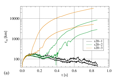
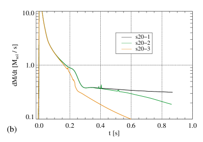
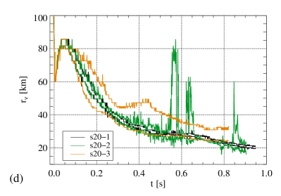
Figure 1: Comparison of quantities characterizing the three models, differentiated by colour, as functions of time. Panel (a): minimum and maximum shock radii as a function of time. Panel (b): mass accretion rate, measured at the shock radius. Panel (c): mass of the PNS as a function of time. Panel (d): minimum and maximum radii of the electron-neutrinosphere.

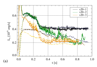
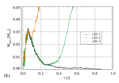
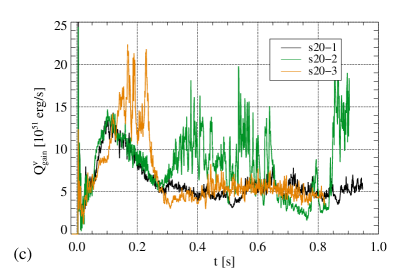
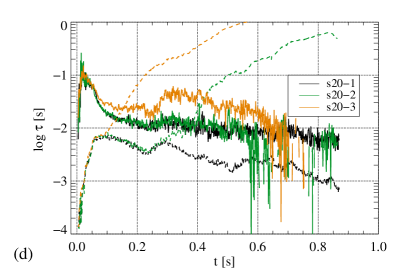
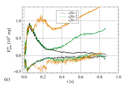
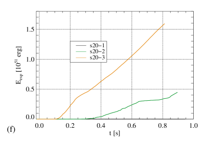
Figure 2: Continuation of Fig. 1. Panel (a): lab-frame neutrino luminosities measured at a radius of $R_{\mathrm{Lum}}=500\,\textrm{km}$; solid, dashed, and dash-triple-dotted lines correspond to $\nu_{e}$, $\bar{\nu}_{e}$, and $\nu_{X}$, respectively. Panel (b): mass contained in the gain layer. Panel (c): heating rate in the gain layer. Panel (d): advection (dash-triple-dotted lines) and heating (solid lines) time scales. Panel (e): internal (solid lines) and total (dashed-triple-dotted lines) energies in the gain layer. Panel (f): diagnostic explosion energy as a function of time (no line is visible for the non-exploding model 20-1).

We present a number of global variables characterizing the time evolution of the three models in Figs. 1 and 2. They serve us to explore the differences between models, which will be discussed individually in the following.

3.1 Model s20-1

The model for which the influence of rotation and magnetic fields is negligible, model s20-1, does not explode. As shown in panel (a) of Fig. 1, the shock wave stalls after $t\approx 100\,\textrm{ms}$. Afterwards, it starts to recede slowly, with only a brief episode ($t\approx 240...300\,\textrm{ms}$) in which the shock contraction is interrupted, caused by the lower mass accretion rate (see panel (b)) onto the PNS as the Si interface of the core is falling through the shock. Owing to the accretion, the PNS mass grows steadily and reaches $M_{\mathrm{PNS}}\approx 2.11\,M_{\odot}$ at the end of the simulation (panel (c)). The PNS might be stable against its own self-gravity for several more seconds, but unless an explosion develops will probably collapse to a black hole.

Throughout the entire evolution, the shock is moderately asymmetric with a ratio between maximum and minimum radii fluctuating in the range $6:5\lesssim r_{\mathrm{sh;max}}:r_{\mathrm{sh;min}}\lesssim 8:5$. This asymmetry bears a clear imprint of north-south sloshing modes exciting in the gain layer, with the location of the maximum radius quasi-periodically oscillating from one pole to the other and the equatorial radius showing only small variations.

The surface of the PNS, for which we take the electron-neutrinosphere (panel (d)) as a proxy, continuously contracts from a maximum radius $r_{\nu}\gtrsim 80\,\textrm{km}$ to one of $r_{\nu}\gtrsim 20\,\textrm{km}$ by the end of the simulation at $t=960\,\textrm{ms}$. Owing to the minor degree of rotation, the neutrinosphere is essentially spherical.

The luminosity (Fig. 2, panel (a)) of all flavours after the $\nu_{e}$-burst, which lasts roughly until $t\approx 50\,\textrm{ms}$, remains relatively high until the accretion of the interface of the inner core around $t\approx 250\,\textrm{ms}$. After that point, the lower accretion rate translates into a lower release of gravitational energy in the form of neutrinos. $\nu_{e}$ and $\bar{\nu}_{e}$ are emitted at constant (and almost equal) luminosities, while the luminosity of the heavy-lepton neutrinos gradually decreases.

To further understand the failure of the explosion, we turn our attention to neutrino heating in the gain layer. Along with the contraction of the shock wave, the mass contained in the gain layer (panel (b) of Fig. 2) decreases from a maximum of $M_{\mathrm{gain}}\approx 0.03\,M_{\odot}$ attained at $t\approx 60\,\textrm{ms}$ to below $M_{\mathrm{gain}}\lesssim 0.001\,M_{\odot}$ at the end of the simulation. Except for an initial rising phase, the net neutrino heating integrated over the gain layer (panel (c)), parallels the evolution of the neutrino luminosity and levels off at a value of $Q^{\nu}_{\mathrm{gain}}\approx{5}\times 10^{51}\,\textrm{erg}\sec^{-1}$. Hence, for most of the evolution, the model combines a constant mass accretion rate and a constant neutrino heating rate in a contracting gain layer. A consequence of this evolution is that the gain-layer average of the neutrino heating time scale, defined in terms of the internal and gravitational energy of the gain layer, $E^{\mathrm{int/grav}}_{\mathrm{gain}}$, as

$$\tau_{\mathrm{htg}}=\frac{E^{\mathrm{int}}_{\mathrm{gain}}+E^{\mathrm{grav}}_{\mathrm{gain}}}{Q^{\nu}_{\mathrm{gain}}},$$ (22)

does not significantly fall below $\tau_{\mathrm{htg}}\approx 10\,\textrm{ms}$ (see Fig. 2, panel (d)). The dwell time, $\tau_{\mathrm{adv}}$, i.e., the value of the integral $\tau_{\mathrm{adv}}(\theta)=\int_{\mathrm{gain\ layer}}\mathrm{d}r/v^{r}$ averaged over polar angles, is shorter at all times. It increases to a first maximum at $t\approx 120\,\textrm{ms}$ and then decreases as the shock radii decrease faster than the gain radii. The subsequent slight expansion of the shock wave increases the width of the gain layer. The corresponding growth of $\tau_{\mathrm{adv}}$, however, is not enough to reach the heating time scale, and no explosion is launched. After $t\approx 300\,\textrm{ms}$, the shock contraction sets in again, and $\tau_{\mathrm{adv}}$ decreases. Even though it eventually rises again towards the end of the simulation, it never exceeds $\tau_{\mathrm{htg}}$. The internal energy of the gain layer (Fig. 2, panel (e)) shows a steady decline after $t\approx 60\,\textrm{ms}$, while its total energy increases from a minimum obtained at the same time, but without ever attaining positive values. Thus, the gain layer is gravitationally bound at all times, disfavoring shock revival.

3.2 Model s20-2

The most important differences of model s20-2 from s20-1 are its fairly fast rotation and strong field. We refer to panel (a) of Fig. 3 for the evolution of the specific angular momentum contained in different layers of the PNS of this model and model s20-3. The temporal evolution of $j$ shows a growth during the first epoch of the simulation and more or less constant values afterwards. From the innermost core with $\rho\geq 10^{14}\,\textrm{g\,cm}^{-3}$, $j$ increases towards the PNS surface where it assumes a value of $j\sim 10^{15}\,\textrm{cm}^{2}/\sec$, which is sufficient to alter the dynamics of these regions.

The magnetic field, on the other hand, is strongest in the centre and weakest at the surface (panel (b) of Fig. 3). However, even there, $b$ reaches an average strength of $b\sim 10^{12}\,\textrm{G}$, dominated by the toroidal component with a relatively weak poloidal component (bottom panel). Locally, it is even stronger which, as we shall see below, has important dynamical consequences.

Early on, model s20-2 evolves very similarly to model s20-1. The minimum and maximum radii of shock and electron-neutrinosphere, the accretion rate and the neutrino luminosities as well as the mass and neutrino heating rate in the gain layer and the time scales of advection and neutrino heating and the resulting energies show only stochastic deviations from the model discussed above (see Fig. 1 and 2).

Unlike in model s20-1, the accretion of the first interface at $t\approx 250\,\textrm{ms}$ triggers an explosion. The expansion of the shock radii setting in at $t\approx 220\,\textrm{ms}$ is sustained and, rather than turning into another epoch of contraction, accelerates, reaching a maximum radius of $r=1000\,\textrm{km}$ about 200 ms after shock revival. The minimum shock radius increases in a similar fashion as the maximum, albeit delayed by about 200 ms. The explosion geometry is clearly bipolar with an essentially symmetric pair of outflows along the rotational axis and downflows at low latitudes. With accretion occurring only under a limited range of angles, the mass accretion rate gradually drops, reducing the neutrino luminosities. Furthermore, the PNS mass grows slower than for model s20-1. At $t=900\,\textrm{ms}$, it is still below $2\,M_{\odot}$, i.e., about $0.1M_{\odot}$ less than in the former model. The diagnostic explosion energy, $E_{\mathrm{exp}}$, i.e. the total (internal, kinetic, magnetic plus gravitational) energy energy of gravitationally unbound, regions (Fig. 2, panel (f)) is continuously rising after the onset of the evolution. Hence, it is still not converged by the end of the simulation and the final value will exceed that of $E_{\mathrm{exp}}\approx{4.6}\times 10^{50}\,\textrm{erg}$ we find at $t\approx 900\,\textrm{ms}$.

The diagnostic quantities show behaviours consistent with the development of an explosion. Around the time of shock revival, the neutrino heating rate in the gain layer increases. While this increase is not directly reflected in the heating time scale, we see a growth of the dwell time until it exceeds the heating time. The internal energy of the gain layer increases and the total energy eventually becomes positive.

To fully understand the mechanism leading to the explosion, we must, however, go beyond these global variables and pay closer attention to the details of the dynamics of the model. Such an approach is required because of the asymmetries of the core. The fact that the explosion starts at the poles while the equatorial regions are far from shock runaway makes for a poor correlation between angularly integrated quantities and the dynamics. We see this, e.g., in the fact that the equality between advection and heating times, is reached around $t\approx 350\,\textrm{ms}$, i.e. about 100 ms after the first signs of the beginning of the explosion, viz. the initiation of the shock expansion at $t\approx 250\,\textrm{ms}$.

Hence, we examine the dynamics of the south polar region where the explosion is launched slightly earlier than at the north pole. In Fig. 4, panel (a), we compare the evolution of the radial velocity along the south pole at times $t\in[50,300]\,\textrm{ms}$ after bounce for models s20-1 (top part of the panel) and s20-2 (bottom half). Until the drop in mass accretion rate at $t\approx 250\,\textrm{ms}$, the post-shock region of both models is characterized by downflows (reddish colours) with upflows (blue) showing up only occasionally. This pattern does not change significantly after that time, i.e., in the brief period during which the shock wave of model s20-1 expands. For model s20-2, on the other hand, the onset of shock expansion is marked by a clear predominance of positive radial velocities. Their large-scale nature, connecting the vicinity of the neutrinosphere (black line) and the shock wave, suggests to search for the mechanism driving shock revival near the PNS.

Around the time of shock revival, the conditions in model s20-2 undergo an important change: the magnetic pressure, before mostly smaller than the gas pressure, achieves and exceeds thermal equipartition. The growth of the parameter $\beta^{-1}=P_{\mathrm{mag}}/P_{\mathrm{gas}}$, shown in panel (b) of Fig. 5, to values $\beta^{-1}\gtrsim 1$ coincides with the development of outflows in model s20-2, whereas it does not happen in the less magnetized model s20-1. Hence, the structure of the polar region cannot be understood without taking into account the magnetic field.

The field can be described in terms of flux tubes as displayed in Fig. 5. Inside the neutrinospheres (pink lines), the field is concentrated between convective cells, in particular along the axis. At the surface of the PNS, we find a layer of enhanced magnetic field with, apart from the polar region, a strong $\theta$-component. This layer is connected to the pre-shock field by various flux tubes threading the gain layer, where they are advected, stretched, and folded by the fluid flow. The magnetic field is too weak to react back on the flow for model s20-1 at all times and for s20-2 before $t\approx 250\,\textrm{ms}$. In these cases, the dynamics of the flux tubes is highly stochastic with field lines following the rise and fall of matter. The result is a complex pattern of field lines and the appearance, merger, and disruption of hot bubbles such as the ones shown by the yellow and red colours in panel (b) Fig. 5 for model s20-1.

The super-equipartition field developing in model s20-2 (see the right part of panel (b) of Fig. 4) takes the form of a rather thick radial flux tube around the axis. In contrast to the patterns at lower latitudes, this flux tube is maintained as a coherent structure for a very long time. The enhanced magnetic pressure leads to a sideways expansion of the gas until the total, i.e. thermal plus magnetic, pressure is matched with the environment. Consequently, the gas in the flux tube has a lower density than the surroundings, as we see, e.g., in the white density contour bending towards lower radii, $r\approx 70\,\textrm{km}$ at the axis in the right part of panel (b). Hence, buoyancy forces lead to the rise of gas along the field lines.

Additionally, the reduction of gas density and internal energy causes the gas to lose less energy by neutrino emission and shifts the boundary between net heating and cooling towards lower radii. Within a few tens of ms after its onset, this process is effective along the entire length of the radial flux tube, i.e. starting immediately outside the neutrinosphere. After $t\approx 300\,\textrm{ms}$, the gain radius has receded to the surface of the PNS. Hence, gas is exposed to intense neutrino heating starting at very low radii as it is ejected. Furthermore, $\bar{\nu}_{e}$ are emitted with slightly higher luminosities and mean energies than $\nu_{e}$. Therefore, they are absorbed by the matter at higher rates. Consequently, matter is (re-)leptonized as it enters the region where it is injected into the outflow. This mode of launching the explosion generates an outflow of high entropy.

The processes described here are at work at both poles and generate outflows along the rotational axis between which accretion onto the PNS proceeds (see the low-entropy regions close to the equator in Fig. 6). The accretion streams possess a stochastic nature and fall onto the PNS with varying geometries and at different angles. For most of the time, they are situated close to the equator, but if one of them moves to a pole, it may suppress the acceleration of the ejecta. This happens at the north pole at $t\approx 500\,\textrm{ms}$. The system then loses its approximate equatorial symmetry. The southern outflow continues progressing in the same way as before, while its northern counterpart slows down as no more energy is injected at its base. About 400 ms later, the north polar engine becomes active again. At $t\approx 835\,\textrm{ms}$ (Fig. 6, right part), the outflows have reached radii of $r\approx 3000\,\textrm{km}$ and $r\approx 5400\,\textrm{km}$ at the north and south poles, respectively. By the end of the simulation, these values increase to $r\approx 4000\,\textrm{km}$ and $r\approx 8400\,\textrm{km}$.

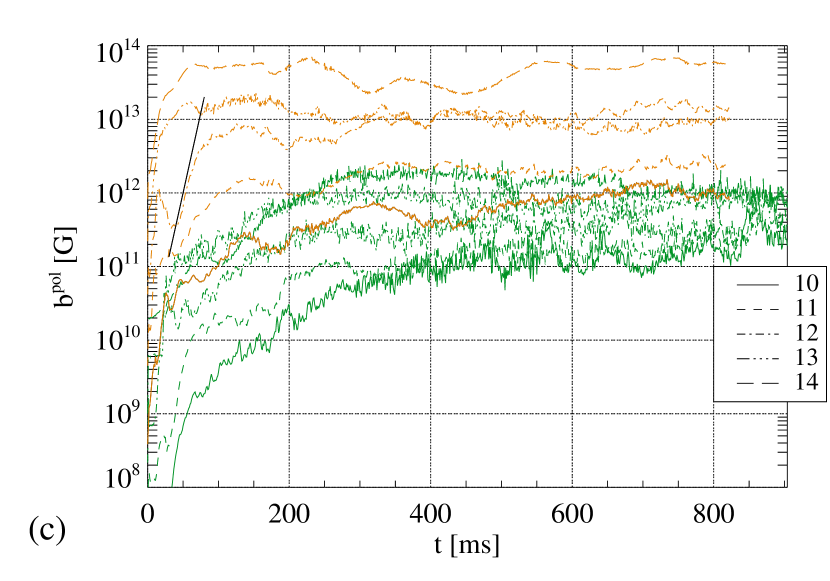
Figure 3: Panel (a): specific angular momentum of models s20-2 (green lines) and s20-3 (orange) as functions of time. Different lines correspond to averages over layers with densities $\log_{10}(\rho\,[\textrm{g\,cm}^{-3}])\in[10,14]\,$, as indicated in the legend. Panel (b): the average magnetic field strength as a function of time for the same layers of the two models. Panel (c): the same as before, but for the average poloidal magnetic field strength. We add an exponential function (solid black line) to indicate the phase of MRI growth in the envelope of the PNS of model s20-3.

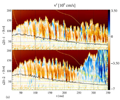
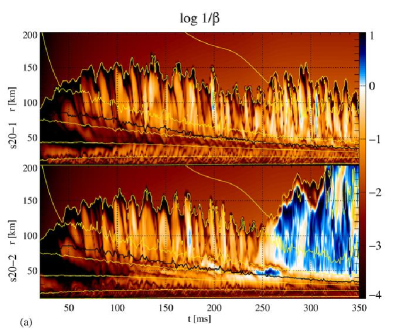
Figure 4: Evolution of the radial velocity (panel (a)) and the inverse plasma-$\beta$ parameter (panel (b)) along the south pole of models s20-1 (upper parts of the panels) and s20-2 (lower parts). In both panels, the black lines represent the gain radius, while the yellow lines are iso-density contours.

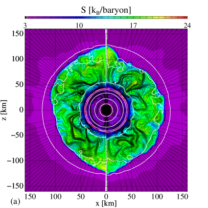
Figure 5: Maps of the specific entropy (colour scale) of models s20-1 (left parts of the three panels) and s20-2 (right parts). The additional lines are magnetic field lines (thin black), density contours (white), and the three neutrinospheres (pink). The times of the snapshots are, from left to right, $t=256$ (panel (a)) and $296\,\textrm{ms}$ (panel (b)).

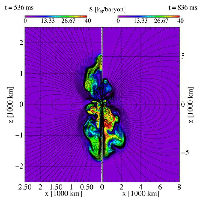
Figure 6: Maps of the specific entropy and magnetic field lines of model s20-2 at two times long after the onset of the explosion as indicated in the panel.

3.3 Model s20-3

The evolution of model s20-3 is affected critically by the rapid rotation. As we see in panel (a) of Fig. 3, the specific angular momentum of the core exceeds that found in model s20-2 by about an order of magnitude, rising to $j\gtrsim 10^{16}\,\textrm{cm}^{2}/\sec$ in the outer layers. Compared to model s20-2, $j$ has a more complex time evolution in the outer layers with a pronounced dip around $t\approx 250\,\textrm{ms}$. The total rotational energy increases monotonically from $E^{\mathrm{rot}}\approx{2}\times 10^{51}\,\textrm{erg}$ shortly after bounce to $E^{\mathrm{rot}}\approx 10^{52}\,\textrm{erg}$ at the end of the simulation.

In the first few tens of milliseconds, the average magnetic field rises very quickly in all layers of the PNS (Fig. 3, panel (b)). This rise is rather a consequence of the rapid infall of magnetized matter and its accumulation on the PNS than of amplification occurring in the PNS. Immediately after bounce, the poloidal magnetic field (Fig. 3, panel (c)) is far stronger than that of model s20-2. However, rather quickly the field growth ceases and, in particular, in the innermost layers the field decreases temporarily until $t\sim 300\,\textrm{ms}$. The corresponding layers of model s20-2 amplify the field for a longer time with the consequence that the initially weaker magnetized model develops a stronger field at layers above $\rho\gtrsim 10^{13}\,\textrm{g\,cm}^{-3}$. The premature stop of field amplification and hence the inversion between the two models is caused mainly by the magnetic field of model s20-3 trying to enforce rigid rotation in the central regions and slowing down the winding of poloidal into toroidal field. The field on the PNS surface, however, decreases less strongly and exceeds $b\sim 10^{12}\,\textrm{G}$. Panel (c) of Fig. 3 demonstrates that the decrease of the total field strength and the partial inversion of the ordering between models s20-3 and s20-2 only affect the toroidal field. The poloidal component, on the other hand, is stronger for model s20-3 than in the corresponding layers of model s20-2 at all times.

Model s20-3 explodes considerably earlier thanmodel s20-2. The shock begins to expand from a radius around $r_{\mathrm{sh}}\approx 170\,\textrm{km}$, which is similar to the stagnation radius of the other models, at the south pole at $t\approx 100\,\textrm{ms}$ and about 15 ms later also at the north pole (cf. Fig. 1). The explosion shock travels very fast. Within a time of 300 ms, the shock wave expands to a radius $r\approx 1000\,\textrm{km}$. Its pattern speed is at that point $v_{\mathrm{sh}}\approx 0.15\,c$ and increases even somewhat afterwards, and the flow speed reaches $v\approx 0.4\,c$. The mass and energy of the unbound ejecta are rising approximately linearly after $t\approx 400\,\textrm{ms}$ at rates $\dot{M}_{\mathrm{ej}}\sim 0.55M_{\odot}/\sec$ and $\dot{E}_{\mathrm{ej}}\sim{2}\times 10^{51}\,\textrm{erg}/\sec$ and reach values of $M_{\mathrm{ej}}\approx 0.45\,M_{\odot}$ and $E_{\mathrm{ej}}\approx{2.1}\times 10^{51}\,\textrm{erg}/\sec$, respectively, at the end of the simulation. We note that the mass and energy are still rising at that time and, hence, these values should be interpreted as lower bounds on the final ones. The same statement holds for the diagnostic energy, which reaches $E_{\mathrm{exp}}\approx{1.6}\times 10^{51}\,\textrm{erg}$ at $t\approx 800\,\textrm{ms}$ and does not show any sign of reducing the rate at which it grows.

After the explosion starts, the mass accretion rate across the shock, thus far dropping at the same rate as in models s20-1/2, is reduced even further. Like in model s20-2, the explosion does not spell an end to accretion as matter is still falling onto the PNS at low latitudes. Consequently, the PNS mass increases throughout the entire simulation, although always remaining lower than in the other models. The reduced accretion rate translates into lower neutrino emission. After the accretion of the core interface at $t\approx 250\,\textrm{ms}$, the luminosities of $\nu_{e}$ and $\bar{\nu}_{e}$ stabilize at slightly more than half the corresponding values of the non-exploding model s20-1, and those of the heavy flavours are almost as large as the neutrinos of electron type. We note, however, that the luminosities are slightly below those of model s20-1 even before the onset of the explosion. Although during this early phase, mass falls through the shock wave at the same rate as in the other models, the partial centrifugal support leads to a more aspherical shape of the PNS with a higher equatorial radius. As a consequence, the same mass accretion rate corresponds to a lower release rate of gravitational binding energy and, hence, less neutrino emission. This effect becomes more pronounced at later times when the minimum (i.e., polar) radius of the PNS contracts similarly to the PNS radii of the other two models, while the maximum (i.e., equatorial) radius shrinks much slower and during a period of almost 150 ms starting at $t\approx 280\,\textrm{ms}$ even expands slowly (see Fig. 1, panel (d), for $r_{\nu}$). The axis ratio of the electron-neutrinosphere assumes a peak of $\approx 17:10$ during this expansion phase to later settle to a value around $13:10$.

As in the case of model s20-2, the global variables describing the gain layer turn out to be insufficient for understanding the explosion mechanism. We find that in the run-up to the explosion, the mass and the internal energy contained in the gain layer behave very similarly to the other models and start to deviate only after the shock is revived. The neutrino heating rate is, in fact, smaller, leading to a larger heating time scale (orange lines in panel (c) and panel (d) of Fig. 2). Equality between heating and advection times is only reached once the shock has already travelled to more than 1000 km.

The explosion, thus, is started at a time when the ram pressure of the pre-shock matter is still too strong for shock revival in model s20-2 even though the neutrino emission is reduced w.r.t. that model. Consequently, neutrino heating cannot be the most important contribution to the explosion mechanism.

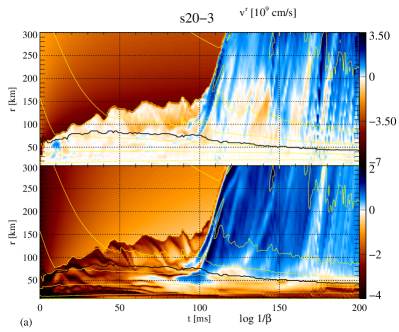
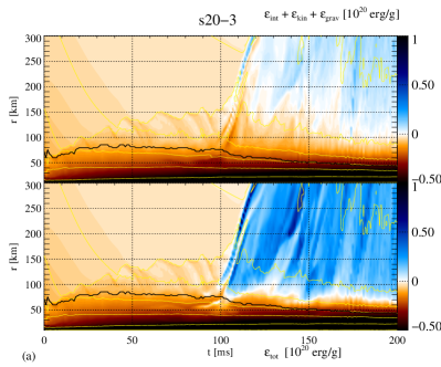
Figure 7: Panel (a): evolution of the radial velocity (top half) and the inverse plasma-$\beta$ parameter along the south pole of model s20-3 (bottom half). Panel (b): the same for the specific total energy without (top) and with (bottom) the magnetic contribution. In both panels, the black lines represent the gain radius, while the yellow lines are iso-density contours.

The shock runaway sets in with matter obtaining large positive velocities (blue regions in the top part of Fig. 7 panel (a)). The ejected matter is threaded by a mostly radial magnetic field whose pressure exceeds the gas pressure by up to more than one order of magnitude (bottom part of the same panel). The outward moving matter achieves positive total energies (blue regions in Fig. 7 panel (b)) close to the gain radius. The important contribution of the magnetic field to unbinding these fluid elements is highlighted by a comparison between the total energy including (bottom part of panel (b) of Fig. 7) or not including (top part of the same panel), the magnetic energy contribution. The latter is in general significantly smaller as well as positive only outside a much larger radius than the former. This difference strengthens the suggestion that the magnetic field, rather than neutrino heating, is primarily responsible for the explosion. The particular strength of the strong magnetic field in the polar region is a result of the contraction of the magnetic flux creating a very strong radial component oriented along the symmetry axis. Other effects such as differential rotation generating a toroidal component or the MRI, which operates further inside the core, are not as important. The explosion mechanism bears some resemblence to the one found by [50] in non-rotating cores. This similarity points towards a larger role of the magnetic field than of the rotation in this shock revival.

The maps displayed in panel (a) of Fig. 8 show the core briefly before and after launching the explosion. At $t\approx 70\,\textrm{ms}$, the PNS is surrounded by a gain layer in which hydrodynamic instabilities produce non-spherical flows and hot bubbles of intermediate sizes appear for brief periods of time and where the evolution and amplification of the magnetic field follows the dynamics of the flow. The feedback of the field on the flow, weak at most locations throughout the gain layer, is important in several smaller regions. The first of those consists of strong sheets of anti-parallel field lines form at intermediate latitudes at the PNS surface. They form, as we see in panel (a) of Fig. 9, at strong negative derivatives w.r.t. $\varpi$ of the angular velocity, which inside the PNS has a roughly cylindrical profile. The magnetic field grows in these structures and leads to the transport of angular momentum reflected in the distortion of the $\Omega$-profile. Their location, shape, and orientation suggest an interpretation as channel modes of the magneto-rotational instability (MRI). This interpretation is consistent with the presence of strongly negative radial gradients of the angular velocity, satisfying the criterion for MRI growth. The latter, in its most basic form (for simplicity, we only focus on the non-convective magneto-shear modes of [49]) predicts that the MRI grows in regions fulfilling the condition $\mathcal{R_{\varpi}}=\varpi\partial_{\varpi}\Omega^{2}<0$ ($\varpi$ is the cylindrical radius). The growth rate of the fastest growing modes of the MRI, given by $\omega_{\mathrm{FGM}}=-\mathcal{R}_{\mathrm{\varpi}}/(4\Omega)$, is shown in the left part of panel (b) of Fig. 9 at $t=85\,\textrm{ms}$. While the values vary strongly across the core, the predicted growth rate in many locations is very high with $\omega_{\mathrm{FGM}}$ in the range of at least several $100\,\sec^{-1}$. On average, lower radii correspond to higher growth rates. Such high values agree with the exponential growth of the (poloidal) magnetic field in the density range $10^{11}\,\textrm{g\,cm}^{-3}<\rho<10^{13}\,\textrm{g\,cm}^{-3}$ (panels (b,c) of Fig. 3). As a demonstration, we added an exponential function with a growth rate of $\omega=100\,\sec^{-1}$ (solid black line) to the curve showing the growth of the poloidal field strength in the density range $10^{12}\,\textrm{g\,cm}^{-3}<\rho<10^{13}\,\textrm{g\,cm}^{-3}$. Furthermore, our grid is sufficiently fine to resolve the fastest growing MRI modes, whose length scales are several km. The right part of panel (b) of Fig. 9 depicts the variable $\Lambda_{\mathrm{FGM}}=2\pi c_{\mathrm{A}}^{\mathrm{pol}}/\sqrt{\mathrm{abs}(-\mathcal{R}_{\mathrm{\varpi}})}$ which is equal to theoretical wavelength of the fastest growing mode, $\lambda_{\mathrm{FGM}}=2\pi c_{\mathrm{A}}^{\mathrm{pol}}/\sqrt{-\mathcal{R}_{\mathrm{\varpi}}}$ in unstable regions, in units of the local grid width, $\Delta r$, where $c_{\mathrm{A}}^{\mathrm{pol}}$ is the Alfvén speed corresponding to the poloidal magnetic field component. In the regions of fastest MRI growth, the wavelength typically exceeds several km, which is in general comparable to or larger than the local grid width. We note, however, that there are regions where the $\lambda_{\mathrm{MRI}}$ is under-resolved. The MRI is better resolved at larger radii. There, however, the growth rate is rather low. We typically cover $\lambda_{\mathrm{FGM}}$ by a few grid cells, which, together with geometrical effects such as the orientation of the field w.r.t. the gradient of $\Omega$ and the neglect of the thermal stratification, accounts for a reduction of the numerical growth rate w.r.t. the theoretical predictions. We note that the distributions of both the growth rate and the wavelength bear the imprint of the channel modes that at this time have already developed and modified the rotational profile. Despite the simplifications entering our analysis, the 2d maps in Fig. 9 support the likely possibility that the MRI is resolved and operating in model s20-3, at least initially in the form of channel modes.

After their formation, the interior end points of these channel modes tend to converge at the polar axis as, e.g., at $t=105\,\textrm{ms}$ around $z=\pm 40\,\textrm{km}$ (Fig. 8, right part of panel (a)). This convergence further enhances the quite strong field that is already there and generates a strong increase of the magnetic pressure. The magnetic pressure is strong enough to overcome the ram pressure of the surrounding matter and finally drives a polar outflow containing strongly magnetized gas (cf.  the distribution of the specific entropy at $t=120\,\textrm{ms}$ in the panel (a) of Fig. 8).

The magnetic forces accelerate matter above the PNS surface into collimated outflows during the entire run of the simulation. The rate at which they transfer energy to the gas is sustained at values above $10^{50}\textrm{erg}/\textrm{s}$ and is highly variable, leading to a rich substructure of faster and slower fluid elements. We find at $t=200\,\textrm{ms}$ (Fig. 8, panel (b)) regions of high entropy along the axis of the outflow, which 400 ms later have intensified. At that later time, we also note the formation of reverse shocks situated at $z\sim+4000\,\textrm{km}$ separating hot matter outside from cooler gas to the interior (visible as the rear end of the red region in the right part of the panel).

The region above the poles of the PNS continues to inject mass from an equatorial accretion stream that separates the north and south outflows into the polar outflows. However, by the end of the simulation, its mass, $M_{\mathrm{PNS}}\approx 1.93\,M_{\odot}$, is still far from the threshold for instability against collapse to a black hole. Based on the mass accretion rates at that point and taking into account the centrifugal stabilization, we estimate that the PNS can maintain its stability for several seconds, if not indefinitely.

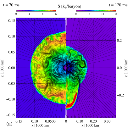
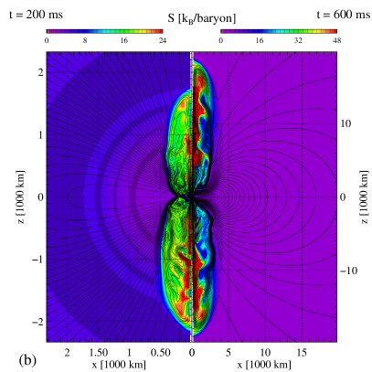
Figure 8: Maps of the specific entropy (colour scale) and field lines (black) of model s20-3 for four different times as indicated in the panels.

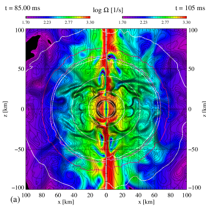
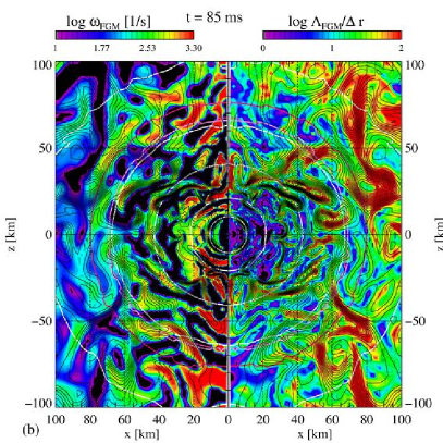
Figure 9: Panel (a): close-up on the PNS of model s20-3 at the two indicated times. The angular velocity is displayed in colours. Field lines are black, and white and pink lines are contours of density ($\rho=10^{14,13,...}\,\textrm{g\,cm}^{-3}$) and the three neutrinospheres, respectively. Panel (b): growth rate, $\omega_{\mathrm{FGM}}$, and wave length, $\Lambda_{\mathrm{FGM}}$, of the fastest growing MRI mode relative to the grid width, $\Delta r$, in model s20-3 at $t=85\,\textrm{ms}$.

4 Summary and conclusions

Increasingly sophisticated multidimensional core collapse simulations of large sets of stars with state-of-the-art neutrino transport are getting closer to an explanation of the mechanisms that produce successful CCSN explosions or non-exploding cores resulting in collapse to black holes. However, a small fraction of all progenitors may possess strong magnetic fields that cannot be ignored as is commonly done in the later simulations, in particular when combined with rapid rotation. However, studies of magneto-rotational core collapse have to face the problem that one-dimensional stellar evolution modelling only provides limited information on the magnetic field and rotation of the pre-collapse cores. Therefore, profiles of magnetic field and rotational velocity are commonly assumed for cores that are otherwise evolved to the pre-collapse state without magnetic fields and rotation. Thus, these studies were able to identify various MHD processes that may in general play a role on the explosion dynamics, but could only in a few cases arrive at detailed conclusions for specific progenitors.

Lacking stellar evolution results for magnetized, rotating versions of the star under consideration, we worked in the same framework to study the influence of rotation and magnetic fields on the evolution of the core of a star of an initial mass of $M=20\,M_{\odot}$ by means of special relativistic axisymmetric MHD simulations including an approximately relativistic gravitational potential and a spectral two-moment neutrino transport. We compared three models with the same distribution of density, electron fraction, and temperature, but different strength of the magnetic field and different angular velocities.

The first of our models, s20-1, starts with negligible rotation and magnetic field. This model behaves essentially as if there were no rotation and magnetic fields at all. About 100 ms after core bounce, the shock wave stagnates before beginning to contract gradually. No explosion is achieved, even though conditions for shock revival, as measured in the ratio between the time scale for advection of fluid elements through the gain layer and the time scale for neutrino heating, improve when the ram pressure at the shock decreases after the accretion of the surface of the iron core. Though the initial magnetic field is amplified both in the PNS and in the gain layer by convection and the SASI, it never reaches a strength sufficient to affect the evolution.

We computed model s20-2, a version of the model with a $j$-constant rotational law, a central angular velocity of $\Omega_{0}=0.1\,\textrm{s}^{-1}$ and the same magnetic fields as model s20-1, viz. $B_{0}^{\mathrm{p,\phi}}=10^{10,11}\,\textrm{G}$ for the poloidal and toroidal components, respectively. Compared to estimates from stellar evolution theory, the field strength is strong, but not exceedingly so. The specific angular momentum increases with radius to values of $j\sim 10^{15}\,\textrm{cm}^{2}\,\textrm{s}^{-1}$, i.e. lies below the values of $j\sim 3\times 10^{16}\,\textrm{cm}^{2}\,\textrm{s}^{-1}$ considered the threshold for the formation of a GRB central engine within the collapsar model [33].

The influence of rotation and magnetic fields lead to a deviation of the evolution of model s20-2 from model s20-1 after the accretion of the silicon shell. The contraction of the shock wave is stopped and a bipolar explosion is launched. Rapid, albeit subrelativistic, outflows develop along the rotational axis while downflows continue at lower latitudes. Neutrino heating, though certainly playing its role in the explosion mechanism, does not differ significantly from the non-exploding model s20-1, as both the total luminosities and heating rates are very similar in both models. The fact that model s20-2 develops an explosion at a neutrino luminosity, which is insufficient in s20-1, is consistent with the findings of [23] who show that rotation tends to reduce the critical luminosity for shock revival. Striking differences at the local level can explain the different evolution of the models. The outflows are launched from a region of strongly enhanced magnetic field, whose pressure becomes equal to and even greater than the gas pressure, close to the neutrinosphere of the core. Magnetic buoyancy in a thick radial flux tube accelerates gas radially along the polar axis. The explosion found in this model is, at least during the simulated time, of moderately high energy: the diagnostic explosion energy reaches about $E_{\mathrm{exp}}\approx{4.6}\times 10^{50}\,\textrm{erg}$, but can be expected to increase further.

Model s20-3, with ten times faster rotation and a ten times stronger poloidal magnetic field than, but the same toroidal field as, model s20-2, explodes already at $t\approx 100\,\textrm{ms}$. The explosion shows little contribution by neutrino heating. In fact, the rapid rotation reduces the neutrino luminosity, which makes a neutrino-driven explosion more unlikely (cf. [62]). Nevertheless, the model is able to overcome the high ram pressure of the infalling matter during the accretion of the iron core due to a strong, super-equipartition field along the rotational axis. Beyond compression, hydrodynamic instabilities, and winding of poloidal field, we also find field amplification by the MRI in this model in the form of a very rapid rise of the field strength produced by the geometrical convergence of MRI channel modes along the rotational axis and close to the surface of the PNS. The properties of these modes as found in the simulation are in reasonable agreement with the theoretical predictions for the magneto-shear modes of the MRI. Our numerical grid covers each wavelength (in the region of interest, typically a several km) by a few grid cells. This means the MRI is resolved, though in the regions of fastest growth only fairly marginally. In the weaker magnetized and slower rotating model s20-2, the grid would also suffice to resolve the MRI. There, however, the growth rates are much lower, and any possible MRI activity would be hidden behind the complex dynamics dominated by other effects.

In model s20-3, the rotation leads to a notable flattening of the PNS with a final equator-to-pole axis ratio of $13:10$, while the spin of model s20-2 is too slow to affect the shape significantly. Both PNSs rotate differentially at the end of the simulation. Over a large fraction of the PNS volume, the angular velocity profile is cylindrical. The magnetic field decreases from the center to the surface by about 2 to 3 orders of magnitude in strength. In both cases, it is dominated by the toroidal component. The poloidal components possess average surface strengths between a few times $10^{11}\,\textrm{G}$ (s20-2) and $10^{12}\,\textrm{G}$ (s20-3). Both components show a rich substructure and cannot adequately be described by a simple low-order multipole, in line with the findings of [45].

We find that model s20-3 explodes very energetically. Its diagnostic energy grows to $E_{\mathrm{exp}}\approx{1.6}\times 10^{51}\,\textrm{erg}$ at the end of the simulation. The final value is most likely considerably higher as we find still a roughly linear increase of $E_{\mathrm{exp}}$ when the simulation was ended. Such a high energy is similar to values computed by [8] for magnetorotational explosions.

We close by briefly discussing the limitations of our present study. As noted above, the lack of detailed stellar-evolution models with rotation and magnetic fields forces us to artificially add those two components to a spherically symmetric pre-collapse model. Thus, our study belongs to those investigating the fundamental effects of rotation and magnetic fields rather than those able to make predictions for a specific star. As such, the models are only a small part of the possible conditions and a more comprehensive scan of the parameter space might be in order. As far as the simulations are concerned, the most crucial limitation is certainly the assumption of axisymmetry. This restriction makes a difference in the tendency of models to explode without rotation and magnetic fields, but also with rotation only [62]. If magnetic fields are included, the impact is even larger. Hence, a continuation of the study in a three-dimensional setup is required.

References

References

- [1] S. M. Adams, C. S. Kochanek, J. R. Gerke, and K. Z. Stanek. The search for failed supernovae with the Large Binocular Telescope: constraints from 7 yr of data. MNRAS, 469:1445–1455, August 2017.
- [2] S. Akiyama, J. C. Wheeler, D. L. Meier, and I. Lichtenstadt. The Magnetorotational Instability in Core-Collapse Supernova Explosions. ApJ, 584:954–970, feb 2003.
- [3] N. V. Ardeljan, G. S. Bisnovatyi-Kogan, K. V. Kosmachevskii, and S. G. Moiseenko. Two-Dimensional Simulation of the Dynamics of the Collapse of a Rotating Core with Formation of a Neutron Star on an Adaptive Triangular Grid in Lagrangian Coordinates. Astrophysics, 47:37–51, jan 2004.
- [4] N. V. Ardeljan, G. S. Bisnovatyi-Kogan, and S. G. Moiseenko. Magnetorotational supernovae. MNRAS, 359:333–344, may 2005.
- [5] G. S. Bisnovatyi-Kogan, I. P. Popov, and A. A. Samokhin. The magnetohydrodynamic rotational model of supernova explosion. Ap&SS, 41:287–320, jun 1976.
- [6] R. Bollig, H.-T. Janka, A. Lohs, G. Martínez-Pinedo, C. J. Horowitz, and T. Melson. Muon Creation in Supernova Matter Facilitates Neutrino-Driven Explosions. Physical Review Letters, 119(24):242702, December 2017.
- [7] A. Burrows. Colloquium: Perspectives on core-collapse supernova theory. Reviews of Modern Physics, 85:245–261, January 2013.
- [8] A. Burrows, L. Dessart, E. Livne, C. D. Ott, and J. Murphy. Simulations of Magnetically Driven Supernova and Hypernova Explosions in the Context of Rapid Rotation. ApJ, 664:416–434, jul 2007.
- [9] A. Burrows, D. Vartanyan, J. C. Dolence, M. A. Skinner, and D. Radice. Crucial Physical Dependencies of the Core-Collapse Supernova Mechanism. Space Sci. Rev., 214:33, February 2018.
- [10] P. Cerdá-Durán, J. A. Font, L. Antón, and E. Müller. A new general relativistic magnetohydrodynamics code for dynamical spacetimes. A&A, 492:937–953, dec 2008.
- [11] P. Cerdá-Durán, J. A. Font, and H. Dimmelmeier. General relativistic simulations of passive-magneto-rotational core collapse with microphysics. A&A, 474:169–191, oct 2007.
- [12] J. Cernohorsky and S. A. Bludman. Maximum entropy distribution and closure for Bose-Einstein and Fermi-Dirac radiation transport. ApJ, 433:250–255, sep 1994.
- [13] S. M. Couch and C. D. Ott. Revival of the Stalled Core-collapse Supernova Shock Triggered by Precollapse Asphericity in the Progenitor Star. ApJ, 778:L7, nov 2013.
- [14] A. Cristini, C. Meakin, R. Hirschi, D. Arnett, C. Georgy, M. Viallet, and I. Walkington. 3D hydrodynamic simulations of carbon burning in massive stars. MNRAS, 471:279–300, October 2017.
- [15] L. Dessart, A. Burrows, E. Livne, and C. D. Ott. Magnetically Driven Explosions of Rapidly Rotating White Dwarfs Following Accretion-Induced Collapse. ApJ, 669:585–599, nov 2007.
- [16] E. Endeve, C. Y. Cardall, R. D. Budiardja, S. W. Beck, A. Bejnood, R. J. Toedte, A. Mezzacappa, and J. M. Blondin. Turbulent Magnetic Field Amplification from Spiral SASI Modes: Implications for Core-collapse Supernovae and Proto-neutron Star Magnetization. ApJ, 751:26, may 2012.
- [17] E. Endeve, C. Y. Cardall, R. D. Budiardja, and A. Mezzacappa. Generation of Magnetic Fields By the Stationary Accretion Shock Instability. ApJ, 713:1219–1243, apr 2010.
- [18] E. Endeve, C. Y. Cardall, and A. Mezzacappa. Conservative Moment Equations for Neutrino Radiation Transport with Limited Relativity. ArXiv e-prints, dec 2012.
- [19] T. Fischer, I. Sagert, G. Pagliara, M. Hempel, J. Schaffner-Bielich, T. Rauscher, F.-K. Thielemann, R. Käppeli, G. Martínez-Pinedo, and M. Liebendörfer. Core-collapse Supernova Explosions Triggered by a Quark-Hadron Phase Transition During the Early Post-bounce Phase. ApJS, 194:39, June 2011.
- [20] J. F. Hawley and S. A. Balbus. A powerful local shear instability in weakly magnetized disks. III - Long-term evolution in a shearing sheet. IV - Nonaxisymmetric perturbations. ApJ, 400:595–621, dec 1992.
- [21] A. Heger, S. E. Woosley, and H. C. Spruit. Presupernova Evolution of Differentially Rotating Massive Stars Including Magnetic Fields. ApJ, 626:350–363, jun 2005.
- [22] C. J. Horowitz. Weak magnetism for antineutrinos in supernovae. Phys. Rev. D, 65(4):043001, February 2002.
- [23] W. Iwakami, H. Nagakura, and S. Yamada. Parametric Study of Flow Patterns behind the Standing Accretion Shock Wave for Core-Collapse Supernovae. ApJ, 786(2):118, 2014.
- [24] O. Just, M. Obergaulinger, and H.-T. Janka. A new multidimensional, energy-dependent two-moment transport code for neutrino-hydrodynamics. MNRAS, 453:3386–3413, November 2015.
- [25] K. Kotake, H. Sawai, S. Yamada, and K. Sato. Magnetorotational effects on anisotropic neutrino emission and convection in core-collapse supernovae. ApJ, 608:391–404, jun 2004.
- [26] K. Kotake, T. Takiwaki, T. Fischer, K. Nakamura, and G. Martínez-Pinedo. Impact of Neutrino Opacities on Core-collapse Supernova Simulations. ApJ, 853:170, February 2018.
- [27] T. Kuroda, K. Kotake, and T. Takiwaki. Fully General Relativistic Simulations of Core-collapse Supernovae with an Approximate Neutrino Transport. ApJ, 755:11, aug 2012.
- [28] T. Kuroda, T. Takiwaki, and K. Kotake. A New Multi-energy Neutrino Radiation-Hydrodynamics Code in Full General Relativity and Its Application to the Gravitational Collapse of Massive Stars. ApJS, 222:20, February 2016.
- [29] N. Langer. Presupernova evolution of massive single and binary stars. Annual Review of Astronomy and Astrophysics, 50(1):null, 2012.
- [30] J. M. LeBlanc and J. R. Wilson. A numerical example of the collapse of a rotating magnetized star. ApJ, 191:541, 1970.
- [31] E. J. Lentz, S. W. Bruenn, W. R. Hix, A. Mezzacappa, O. E. B. Messer, E. Endeve, J. M. Blondin, J. A. Harris, P. Marronetti, and K. N. Yakunin. Three-dimensional Core-collapse Supernova Simulated Using a 15 M⊙ Progenitor. ApJ, 807:L31, July 2015.
- [32] P. Londrillo and L. del Zanna. On the divergence-free condition in Godunov-type schemes for ideal magnetohydrodynamics: the upwind constrained transport method. \jcop, 195:17–48, mar 2004.
- [33] A. I. MacFadyen and S. E. Woosley. Collapsars: Gamma-Ray Bursts and Explosions in “Failed Supernovae”. ApJ, 524:262–289, oct 1999.
- [34] A. Marek, H. Dimmelmeier, H.-T. Janka, E. Müller, and R. Buras. Exploring the relativistic regime with Newtonian hydrodynamics: an improved effective gravitational potential for supernova simulations. A&A, 445:273–289, jan 2006.
- [35] Y. Masada, T. Takiwaki, and K. Kotake. Magnetohydrodynamic Turbulence Powered by Magnetorotational Instability in Nascent Protoneutron Stars. ApJ, 798:L22, January 2015.
- [36] Y. Masada, T. Takiwaki, K. Kotake, and T. Sano. Local Simulations of the Magnetorotational Instability in Core-collapse Supernovae. ApJ, 759:110, nov 2012.
- [37] D. L. Meier, R. I. Epstein, W. D. Arnett, and D. N. Schramm. Magnetohydrodynamic phenomena in collapsing stellar cores. ApJ, 204:869–878, mar 1976.
- [38] S. G. Moiseenko, G. S. Bisnovatyi-Kogan, and N. V. Ardeljan. A magnetorotational core-collapse model with jets. MNRAS, 370:501–512, jul 2006.
- [39] P. Mösta, C. D. Ott, D. Radice, L. F. Roberts, E. Schnetter, and R. Haas. A large-scale dynamo and magnetoturbulence in rapidly rotating core-collapse supernovae. Nature, 528:376–379, December 2015.
- [40] P. Mösta, S. Richers, C. D. Ott, R. Haas, A. L. Piro, K. Boydstun, E. Abdikamalov, C. Reisswig, and E. Schnetter. Magnetorotational Core-collapse Supernovae in Three Dimensions. ApJ, 785:L29, apr 2014.
- [41] B. Müller, T. Melson, A. Heger, and H.-T. Janka. Supernova simulations from a 3D progenitor model - Impact of perturbations and evolution of explosion properties. MNRAS, 472:491–513, November 2017.
- [42] B. Müller, M. Viallet, A. Heger, and H.-T. Janka. The Last Minutes of Oxygen Shell Burning in a Massive Star. ApJ, 833:124, December 2016.
- [43] E. Müller and W. Hillebrandt. A magnetohydrodynamical supernova model. A&A, 80:147–154, dec 1979.
- [44] K. Nakamura, T. Takiwaki, T. Kuroda, and K. Kotake. Systematic features of axisymmetric neutrino-driven core-collapse supernova models in multiple progenitors. PASJ, 67:107, December 2015.
- [45] M. Obergaulinger and M. Á. Aloy. Evolution of the surface magnetic field of rotating proto-neutron stars. In Journal of Physics Conference Series, volume 932 of Journal of Physics Conference Series, page 012043, December 2017.
- [46] M. Obergaulinger and M. Á. Aloy. Protomagnetar and black hole formation in high-mass stars. MNRAS, 469:L43–L47, July 2017.
- [47] M. Obergaulinger, M. A. Aloy, H. Dimmelmeier, and E. Müller. Axisymmetric simulations of magnetorotational core collapse: approximate inclusion of general relativistic effects. A&A, 457:209–222, oct 2006.
- [48] M. Obergaulinger, M. A. Aloy, and E. Müller. Axisymmetric simulations of magneto-rotational core collapse: dynamics and gravitational wave signal. A&A, 450:1107–1134, may 2006.
- [49] M. Obergaulinger, P. Cerdá-Durán, E. Müller, and M. A. Aloy. Semi-global simulations of the magneto-rotational instability in core collapse supernovae. A&A, 498:241–271, apr 2009.
- [50] M. Obergaulinger, H.-T. Janka, and M. A. Aloy. Magnetic field amplification and magnetically supported explosions of collapsing, non-rotating stellar cores. MNRAS, 445:3169–3199, December 2014.
- [51] E. O’Connor and C. D. Ott. Black Hole Formation in Failing Core-Collapse Supernovae. ApJ, 730:70, apr 2011.
- [52] C. D. Ott, E. Abdikamalov, P. Mösta, R. Haas, S. Drasco, E. P. O’Connor, C. Reisswig, C. A. Meakin, and E. Schnetter. General-relativistic Simulations of Three-dimensional Core-collapse Supernovae. ApJ, 768:115, may 2013.
- [53] M. Rampp and H.-Th. Janka. Radiation hydrodynamics with neutrinos. Variable Eddington factor method for core-collapse supernova simulations. A&A, 396:361–392, dec 2002.
- [54] T. Rembiasz, J. Guilet, M. Obergaulinger, P. Cerdá-Durán, M. A. Aloy, and E. Müller. On the maximum magnetic field amplification by the magnetorotational instability in core-collapse supernovae. MNRAS, 460:3316–3334, August 2016.
- [55] T. Rembiasz, M. Obergaulinger, P. Cerdá-Durán, E. Müller, and M. A. Aloy. Termination of the magnetorotational instability via parasitic instabilities in core-collapse supernovae. MNRAS, 456:3782–3802, March 2016.
- [56] H. Sawai, K. Kotake, and S. Yamada. Numerical Simulations of Equatorially Asymmetric Magnetized Supernovae: Formation of Magnetars and Their Kicks. ApJ, 672:465–478, jan 2008.
- [57] H. Sawai and S. Yamada. The Evolution and Impacts of Magnetorotational Instability in Magnetized Core-collapse Supernovae. ApJ, 817:153, February 2016.
- [58] H. Sawai, S. Yamada, and H. Suzuki. Global Simulations of Magnetorotational Instability in the Collapsed Core of a Massive Star. ApJ, 770:L19, jun 2013.
- [59] S. Scheidegger, T. Fischer, S. C. Whitehouse, and M. Liebendörfer. Gravitational waves from 3D MHD core collapse simulations. A&A, 490:231–241, oct 2008.
- [60] A. W. Steiner, M. Hempel, and T. Fischer. Core-collapse Supernova Equations of State Based on Neutron Star Observations. ApJ, 774:17, sep 2013.
- [61] T. Sukhbold, T. Ertl, S. E. Woosley, J. M. Brown, and H.-T. Janka. Core-collapse Supernovae from 9 to 120 Solar Masses Based on Neutrino-powered Explosions. ApJ, 821:38, April 2016.
- [62] A. Summa, H.-T. Janka, T. Melson, and A. Marek. Rotation-supported Neutrino-driven Supernova Explosions in Three Dimensions and the Critical Luminosity Condition. ArXiv e-prints, August 2017.
- [63] A. Suresh and H.T. Huynh. Accurate monotonicity-preserving schemes with runge-kutta time stepping. \jcop, 136:83–99, 1997.
- [64] Y. Suwa, T. Takiwaki, K. Kotake, and K. Sato. Magnetorotational Collapse of Population III Stars. PASJ, 59:771–785, aug 2007.
- [65] M. Ugliano, H.-T. Janka, A. Marek, and A. Arcones. Progenitor-explosion Connection and Remnant Birth Masses for Neutrino-driven Supernovae of Iron-core Progenitors. ApJ, 757:69, sep 2012.
- [66] C. Winteler, R. Käppeli, A. Perego, A. Arcones, N. Vasset, N. Nishimura, M. Liebendörfer, and F.-K. Thielemann. Magnetorotationally Driven Supernovae as the Origin of Early Galaxy r-process Elements? ApJ, 750:L22, may 2012.
- [67] S. E. Woosley and A. Heger. Nucleosynthesis and remnants in massive stars of solar metallicity. Phys. Rep., 442:269–283, apr 2007.