On Efficient Domination for Some Classes of $H$-Free Bipartite Graphs

Abstract

A vertex set $D$ in a finite undirected graph $G$ is an efficient dominating set (e.d.s. for short) of $G$ if every vertex of $G$ is dominated by exactly one vertex of $D$. The Efficient Domination (ED) problem, which asks for the existence of an e.d.s. in $G$, is known to be $\mathbb{NP}$-complete even for very restricted $H$-free graph classes such as for $2P_{3}$-free chordal graphs while it is solvable in polynomial time for $P_{6}$-free graphs. Here we focus on bipartite graphs: We show that (weighted) ED can be solved in polynomial time for $H$-free bipartite graphs when $H$ is $P_{7}$ or $\ell P_{4}$ for fixed $\ell$, and similarly for $P_{9}$-free bipartite graphs with vertex degree at most 3, and when $H$ is $S_{2,2,4}$. Moreover, we show that ED is $\mathbb{NP}$-complete for bipartite graphs with diameter at most 6.

Keywords: Weighted efficient domination; $H$-free bipartite graphs; $\mathbb{NP}$-completeness; polynomial time algorithm; clique-width.

1 Introduction

Let $G=(V,E)$ be a finite undirected graph. A vertex $v$ dominates itself and its neighbors. A vertex subset $D\subseteq V$ is an efficient dominating set (e.d.s. for short) of $G$ if every vertex of $G$ is dominated by exactly one vertex in $D$; for any e.d.s. $D$ of $G$, $|D\cap N[v]|=1$ for every $v\in V$ (where $N[v]$ denotes the closed neighborhood of $v$). Note that not every graph has an e.d.s.; the Efficient Dominating Set (ED) problem asks for the existence of an e.d.s. in a given graph $G$. The notion of efficient domination was introduced by Biggs [7] under the name perfect code.

The Exact Cover Problem asks for a subset ${\cal F^{\prime}}$ of a set family ${\cal F}$ over a ground set, say $V$, containing every vertex in $V$ exactly once, i.e., ${\cal F^{\prime}}$ forms a partition of $V$. As shown by Karp [24], this problem is $\mathbb{NP}$-complete even for set families containing only $3$-element subsets of $V$ (see problem X3C [SP2] in [23]).

Clearly, ED is the Exact Cover problem for the closed neighborhood hypergraph of $G$, i.e., if $D=\{d_{1},\ldots,d_{k}\}$ is an e.d.s. of $G$ then $N[d_{1}]\cup\ldots\cup N[d_{k}]$ forms a partition of $V$ (we call it the e.d.s. property). In particular, the distance between any pair of distinct $D$-vertices $d_{i},d_{j}$ is at least 3.

In [5, 6], it was shown that the ED problem is $\mathbb{NP}$-complete. Moreover, Lu and Tang [31] showed that ED is $\mathbb{NP}$-complete for chordal bipartite graphs (i.e., hole-free bipartite graphs). Thus, for every $k\geq 3$, ED is $\mathbb{NP}$-complete for $C_{2k}$-free bipartite graphs.

Moreover, ED is $\mathbb{NP}$-complete for planar bipartite graphs [31] and even for planar bipartite graphs of maximum degree 3 [16] and girth at least $g$ for every fixed $g$ [33]. Thus, ED is $\mathbb{NP}$-complete for $K_{1,4}$-free bipartite graphs and for $C_{4}$-free bipartite graphs.

In [10], it is shown that one can extend polynomial time algorithms for Efficient Domination to such algorithms for weighted Efficient Domination. Thus, from now on, we focus on the unweighted ED problem.

In [13], it is shown that ED is solvable in polynomial time for interval bigraphs, and convex bipartite graphs are a subclass of them (and of chordal bipartite graphs). Moreover, Lu and Tang [31] showed that ED is solvable in linear time for bipartite permutation graphs (which is a subclass of convex bipartite graphs). It is well known (see e.g. [14, 25]) that $G$ is a bipartite permutation graph if and only if $G$ is AT-free bipartite if and only if $G$ is ($H_{1},H_{2},H_{3}$,hole)-free bipartite (see Figure 1). Thus, while ED is $\mathbb{NP}$-complete for $(H_{2},H_{3})$-free bipartite graphs (since $H_{2}$ and $H_{3}$ contain $C_{4}$ and $H_{2}$ contains $K_{1,4}$), we will show that ED is solvable in polynomial time for $S_{2,2,2}$-free (and more generally, for $S_{2,2,4}$-free) bipartite graphs.

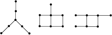
Figure 1: Forbidden induced subgraphs $H_{1}=S_{2,2,2},H_{2},H_{3}$ for bipartite permutation graphs

For a set ${\cal F}$ of graphs, a graph $G$ is called ${\cal F}$-free if $G$ contains no induced subgraph isomorphic to a member of ${\cal F}$. In particular, we say that $G$ is $H$-free if $G$ is $\{H\}$-free. Let $H_{1}+H_{2}$ denote the disjoint union of graphs $H_{1}$ and $H_{2}$, and for $k\geq 2$, let $kH$ denote the disjoint union of $k$ copies of $H$. For $i\geq 1$, let $P_{i}$ denote the chordless path with $i$ vertices, and let $K_{i}$ denote the complete graph with $i$ vertices (clearly, $P_{2}=K_{2}$). For $i\geq 4$, let $C_{i}$ denote the chordless cycle with $i$ vertices.

For indices $i,j,k\geq 0$, let $S_{i,j,k}$ denote the graph with vertices $u,x_{1},\ldots,x_{i}$, $y_{1},\ldots,y_{j}$, $z_{1},\ldots,z_{k}$ (and center $u$) such that the subgraph induced by $u,x_{1},\ldots,x_{i}$ forms a $P_{i+1}$ ($u,x_{1},\ldots,x_{i}$), the subgraph induced by $u,y_{1},\ldots,y_{j}$ forms a $P_{j+1}$ ($u,y_{1},\ldots,y_{j}$), and the subgraph induced by $u,z_{1},\ldots,z_{k}$ forms a $P_{k+1}$ ($u,z_{1},\ldots,z_{k}$), and there are no other edges in $S_{i,j,k}$. Thus, claw is $S_{1,1,1}$, chair is $S_{1,1,2}$, and $P_{k}$ is isomorphic to $S_{0,0,k-1}$.

For a vertex $v\in V$, $N(v)=\{u\in V:uv\in E\}$ denotes its (open) neighborhood, and $N[v]=\{v\}\cup N(v)$ denotes its closed neighborhood. The non-neighborhood of a vertex $v$ is $\overline{N}(v):=V\setminus N[v]$. For $U\subseteq V$, $N(U):=\bigcup_{u\in U}N(u)\setminus U$ and $\overline{N}(U):=V\setminus(U\cup N(U))$.

We say that for a vertex set $X\subseteq V$, a vertex $v\notin X$ has a join (resp., co-join) to $X$ if $X\subseteq N(v)$ (resp., $X\subseteq\overline{N}(v)$). Join (resp., co-join) of $v$ to $X$ is denoted by $v\text{{\footnotesize1}⃝}X$ (resp., $v\text{{\footnotesize0}⃝}X$). Correspondingly, for vertex sets $X,Y\subseteq V$ with $X\cap Y=\emptyset$, $X\text{{\footnotesize1}⃝}Y$ denotes $x\text{{\footnotesize1}⃝}Y$ for all $x\in X$ and $X\text{{\footnotesize0}⃝}Y$ denotes $x\text{{\footnotesize0}⃝}Y$ for all $x\in X$. A vertex $x\notin U$ contacts $U$ if $x$ has a neighbor in $U$. For vertex sets $U,U^{\prime}$ with $U\cap U^{\prime}=\emptyset$, $U$ contacts $U^{\prime}$ if there is a vertex in $U$ contacting $U^{\prime}$.

If $v\not\in X$ but $v$ has neither a join nor a co-join to $X$, then we say that $v$ distinguishes $X$. A set $H$ of at least two vertices of a graph $G$ is called homogeneous if $H\not=V(G)$ and every vertex outside $H$ is either adjacent to all vertices in $H$, or to no vertex in $H$. Obviously, $H$ is homogeneous in $G$ if and only if $H$ is homogeneous in the complement graph $\overline{G}$. A graph is prime if it contains no homogeneous set. In [11, 12, 16], it is shown that the ED problem can be reduced to prime graphs.

It is well known that for a graph class with bounded clique-width, ED can be solved in polynomial time [18]. Thus we only consider ED on $H$-free bipartite graphs for which the clique-width is unbounded. In [20], the clique-width of all classes of $H$-free bipartite graphs is classified. For example, while ED is $\mathbb{NP}$-complete for claw-free graphs (even for ($K_{1,3},K_{4}-e$)-free perfect graphs [30]), the clique-width of claw-free bipartite graphs is bounded.

Based on Lozin’s papers [26, 27, 28, 29] (with coauthors Rautenbach and Volz), the following dichotomy theorem was found by Dabrowski and Paulusma ($H\subseteq_{i}G$ indicates that $H$ is an induced subgraph of $G$):

Theorem 1 ([20]).

The clique-width of $H$-free bipartite graphs is bounded if and only if one of the following cases appears:

1. $H=sP_{1}$, $s\geq 1$;

2. $H\subseteq_{i}K_{1,3}+3P_{1}$;

3. $H\subseteq_{i}K_{1,3}+P_{2}$;

4. $H\subseteq_{i}S_{1,1,3}+P_{1}$;

5. $H\subseteq_{i}S_{1,2,3}$.

Let $d_{G}(x,y)$ denote the distance of $x$ and $y$ in $G$. For graph $G=(V,E)$, its square $G^{2}$ has the same vertex set $V$, and two vertices $x,y\in V$, $x\neq y$, are adjacent in $G^{2}$ if and only if $d_{G}(x,y)\leq 2$. Let $N^{2}(v)=N(N(v))$, i.e., $N^{2}(v)$ is the subset of vertices which have distance 2 to $v$, and correspondingly, $N^{2}(U)$ for $U\subseteq V$ is the set of vertices which have distance 2 to at least one vertex of $U$. The ED problem on $G$ can be reduced to Maximum Weight Independent Set (MWIS) on $G^{2}$ (see e.g. [13, 10, 16, 32] and the survey in [9]).

2 ED in polynomial time for some $H$-free bipartite graphs

2.1 A general approach

A vertex $u\in V$ is forced if $u\in D$ for every e.d.s. $D$ of $G$; $u$ is excluded if $u\notin D$ for every e.d.s. $D$ of $G$. By a forced vertex $u$, $G$ can be reduced to $G^{\prime}$ as follows:

Claim 2.1.

If $u$ is forced then $G$ has an e.d.s. $D$ with $u\in D$ if and only if the reduced graph $G^{\prime}=G\setminus N[u]$ has an e.d.s. $D^{\prime}=D\setminus\{u\}$ such that all vertices in $N^{2}(u)$ are excluded in $G^{\prime}$.

Analogously, if we assume that $v\in D$ for a vertex $v\in V$ then $u\in V$ is $v$-forced if $u\in D$ for every e.d.s. $D$ of $G$ with $v\in D$, and $u$ is $v$-excluded if $u\notin D$ for every e.d.s. $D$ of $G$ with $v\in D$. For checking whether $G$ has an e.d.s. $D$ with $v\in D$, we can clearly reduce $G$ by forced vertices as well as by $v$-forced vertices when we assume that $v\in D$:

Claim 2.2.

If we assume that $v\in D$ and $u$ is $v$-forced then $G$ has an e.d.s. $D$ with $v\in D$ if and only if the reduced graph $G^{\prime}=G\setminus N[u]$ has an e.d.s. $D^{\prime}=D\setminus\{u\}$ with $v\in D^{\prime}$ such that all vertices in $N^{2}(u)$ are $v$-excluded in $G^{\prime}$.

Similarly, for $k\geq 2$, $u\in V$ is $(v_{1},\ldots,v_{k})$-forced,if $u\in D$ for every e.d.s. $D$ of $G$ with $v_{1},\ldots,v_{k}\in D$, and correspondingly, $u\in V$ is $(v_{1},\ldots,v_{k})$-excluded if $u\notin D$ for such e.d.s. $D$, and $G$ can be reduced by the same principle.

In this manuscript, we solve some cases in polynomial time by the following approach: Assume that $G$ has an e.d.s. $D$. Then for any vertex $v\in V$, $|N[v]\cap D|=1$. Assume that $v\in D$ for a vertex $v\in V$, and let $N_{i}$, $0\leq i\leq k$, denote the distance levels of $v$ in $G$ (in particular, $N_{0}=\{v\}$). Since $G$ is bipartite, every $N_{i}$ is independent. Since we assume that $v\in D$ and $D$ is an e.d.s. of $G$ (i.e., the closed neighborhoods of the $D$-vertices form a partition of $V$), all vertices in $N_{1}\cup N_{2}$ are $v$-excluded, and thus we have:

$$D\cap(N_{1}\cup N_{2})=\emptyset.$$ (1)

Here are examples when $v\in D$ is impossible as well as examples for $v$-forced vertices:

Claim 2.3.

Assume that $v\in D$. Then:

• If for some $x\in N_{2}$, $N(x)\cap N_{3}=\emptyset$ then $G$ has no e.d.s. $D$ with $v\in D$.

• If for some $x\in N_{2}$, $N(x)\cap N_{3}=\{y\}$ then $y$ is $v$-forced.

• If for $y\in N_{3}$, $N(y)\cap N_{4}=\emptyset$ then $y$ is $v$-forced.

• If for $y_{1},y_{2}\in N_{3}$, $y_{1}\neq y_{2}$, $N(y_{1})\cap N_{4}=N(y_{2})\cap N_{4}=\emptyset$ and $N(y_{1})\cap N(y_{2})\cap N_{2}\neq\emptyset$ then $G$ has no e.d.s. $D$ with $v\in D$.

Thus, after reducing $G$ by such $v$-forced vertices, for finding an e.d.s. $D$ with $v\in D$, we can assume:

$$\mbox{For every }y\in N_{3},N(y)\cap N_{4}\neq\emptyset.$$ (2)

More generally, for $i\geq 1$, let us write

• $N_{i}^{*}=\{x\in N_{i}:N(x)\cap N_{i+1}\neq\emptyset\}$, and

• $N_{i}^{0}=\{x\in N_{i}:N(x)\cap N_{i+1}=\emptyset\}$,

i.e., $\{N_{i}^{*},N_{i}^{0}\}$ is a partition of $N_{i}$.

For $y_{i}\in D\cap N_{3}$, let $x_{i}\in N_{2}$ and $z_{i}\in N_{4}$ with $x_{i}y_{i}\in E$ and $y_{i}z_{i}\in E$ for $i\in\{1,2\}$ (recall (2)). Clearly, for every pair $y_{1},y_{2}\in D\cap N_{3}$, $y_{1}\neq y_{2}$, we have:

$$x_{1},x_{2},y_{1},y_{2},z_{1},z_{2}\mbox{ induce a }2P_{3}.$$ (3)

Claim 2.4.

Assume that $D\cap N_{3}=\{y_{1},\ldots,y_{k}\}$ for $k\geq 3$ $($recall $(\ref{xN3N4neighb}))$. Then:

• If at least three vertices in $N(D\cap N_{3})\cap N_{2}$, say $x_{1},x_{2},x_{3}$, have private neighbors in $N_{1}$ then there is an $S_{4,4,4}$ in $G$.

• If all of $x_{1},x_{2},x_{3}$ have a common neighbor in $N_{1}$ then there is an $S_{3,3,3}$ in $G$.

• If neither $(i)$ nor $(ii)$ appears then there is an $S_{2,4,4}$ or $S_{3,3,5}$ in $G$.

Proof. $(i)$: Let $u_{i}\in N_{1}$ be the private neighbors of $x_{i}$, $i\in\{1,2,3\}$. Then $v,u_{1},x_{1},y_{1},z_{1}$, $u_{2},x_{2},y_{2},z_{2},u_{3},x_{3},y_{3},z_{3}$ (with center $v$) induce an $S_{4,4,4}$.

$(ii)$: Let $u\in N_{1}$ be a common neighbor of $x_{i}$, $i\in\{1,2,3\}$. Then $u,x_{1},y_{1},z_{1}$, $x_{2},y_{2},z_{2},x_{3},y_{3},z_{3}$ (with center $u$) induce an $S_{3,3,3}$.

$(iii)$: Assume that not all of $x_{1},x_{2},x_{3}$ have private neighbors in $N_{1}$ and there is no common neighbor of $x_{1},x_{2},x_{3}$ in $N_{1}$ (since neither $(i)$ nor $(ii)$ appears). Without loss of generality, let $u\in N_{1}$ be a common neighbor of $x_{1},x_{2}$ such that $ux_{3}\notin E$, and let $u^{\prime}\in N_{1}$ with $u^{\prime}x_{3}\in E$.

If $u^{\prime}x_{1}\in E$ and $u^{\prime}x_{2}\notin E$ then $x_{1},y_{1},z_{1},u,x_{2},y_{2},z_{2},u^{\prime},x_{3},y_{3},z_{3}$ (with center $x_{1}$) induce an $S_{2,4,4}$, and similarly, if $u^{\prime}x_{2}\in E$ and $u^{\prime}x_{1}\notin E$ then $x_{2},y_{2},z_{2},u,x_{1},y_{1},z_{1},u^{\prime},x_{3},y_{3},z_{3}$ (with center $x_{2}$) induce an $S_{2,4,4}$.

Finally, if $u^{\prime}x_{1}\notin E$ and $u^{\prime}x_{2}\notin E$ then $u,x_{1},y_{1},z_{1},x_{2},y_{2},z_{2},v,u^{\prime},x_{3},y_{3},z_{3}$ (with center $u$) induce an $S_{3,3,5}$. Thus, Claim 2.4 is shown. $\diamond$

Recall that we assume that $v\in D$ for a vertex $v\in V$, and $N_{i}$, $1\leq i\leq k$ are the distance levels of $v$. Let

$$G_{i}:=G[\{v\}\cup N_{1}\cup\ldots\cup N_{i}]$$

and assume that

$$D_{i}:=D\cap(\{v\}\cup N_{1}\cup\ldots\cup N_{i})$$

is known as an e.d.s. for $G_{i-1}$. In particular, $D_{0}=D_{1}=D_{2}=\{v\}$. Note that for $i\geq 3$, $D_{i}$ additionally dominates parts of $N_{i}\cup N_{i+1}$.

Let

$$N^{\prime}_{i}:=N_{i}\setminus(D_{i}\cup N(D_{i})).$$

Recall that for any $d,d^{\prime}\in D$, $d\neq d^{\prime}$, $d_{G}(d,d^{\prime})\geq 3$. Thus, for possible $D$-candidates from $N_{i+1}$, we have to exclude $N(D_{i})\cup N^{2}(D_{i})$ from $N_{i+1}$ (recall the notion of $N^{2}(D_{i})$ as in the Introduction), i.e.,

$$W_{i+1}:=N_{i+1}\setminus(N(D_{i})\cup N^{2}(D_{i})).$$

The collection of possible $D$-candidates in $W_{i+1}$ has to dominate $N^{\prime}_{i}$.

Thus, for constructing $D_{i+1}$ from $D_{i}$, for a possible subset $Z_{i+1}\subset W_{i+1}$ such that $Z_{i+1}$ dominates $N^{\prime}_{i}$ (following the e.d.s. property), we have $D_{i+1}=D_{i}\cup Z_{i+1}$.

Finally, if $N_{k}$ is the last distance level of $v$ then $N_{k}\setminus N(D_{k-1})\subset D$ (if there exists an e.d.s. $D$ with $v\in D$).

The stepwise construction of $D_{i+1}$ from $D_{i}$ is possible e.g. when candidates are forced (and the reduction follows): Recall that $D_{1}=\{v\}$ is an e.d.s. for $G_{1}$. Similarly as for $v$-forced vertices, a vertex $u\in W_{i+1}$ is $D_{i}$-forced if $u\in D$ for every e.d.s. $D$ of $G$ with $D_{i}\subset D$, $D_{i}$ being an e.d.s. for $G_{i-1}$.

As in Claim 2.3 $(iii)$ and (2), a non-excluded vertex $x\in N_{i+1}$ (with respect to $D_{i}$) with neighbor in $N^{\prime}_{i}$ is $D_{i}$-forced if $N(x)\cap N_{i+2}=\emptyset$. Thus we can assume that $N(x)\cap N_{i+2}\neq\emptyset$, i.e., $x\in N_{i+1}^{*}$.

One of the helpful arguments is that in some cases, $v$ has only a fixed number of distance levels; for instance, this is the case for $P_{k}$-free bipartite graphs (e.g., for $P_{5}$-free bipartite graphs, we have $N_{4}=\emptyset$) as well as, more generally, for $\ell P_{k}$-free bipartite graphs (but the complexity of ED is still open for $P_{8}$-free bipartite graphs and for $\ell P_{5}$-free bipartite graphs).

A more general case is when for all $i\geq k$, every $x\in N_{i}$ has at most one neighbor in $N_{i+1}$; for instance, this is the case for $S_{1,1,k}$-free bipartite graphs (for which the complexity of ED is still open).

Another more general case is when an e.d.s. $D$ in $G$ has only polynomially many subsets in $N_{i}$, $i\geq 3$. If $v$ has a fixed number of $k$ distance levels $N_{i}$, then, starting with $D_{1}=\{v\}$, for $i:=1$ to $k$, we can produce a polynomial number of $D_{i}$. This can be done for $P_{7}$-free bipartite graphs and for $\ell P_{4}$-free bipartite graphs (see Section 2.2).

If the number of distance levels $N_{i}$ of $v$ is not fixed, it leads to a polynomial time algorithm for ED when e.g. $D$ has polynomially many subsets in $N_{3}$ and for each $D_{i}$, $i\geq 2$, the candidates for $D_{i+1}$ are $D_{i}$-forced. This can be done e.g. for $S_{2,2,4}$-free bipartite graphs (see Section 2.3). A more special case is when for all distance levels $N_{i}$, $i\geq k$ for a fixed number $k$, there is at most one neighbor of $x\in N_{i}$ in $N_{i+1}$, and the number of e.d.s. candidates for $G_{k-1}$ is polynomial. This can be done for $S_{1,2,4}$-free bipartite graphs (see Section 2.3).

2.2 ED in polynomial time for $H$-free bipartite graphs when $H=P_{7}$ or $H=\ell P_{4}$

Recall that ED is $\mathbb{NP}$-complete for $P_{7}$-free graphs but polynomial for $P_{6}$-free graphs (see e.g. [17]). Moreover, for $P_{5}$-free bipartite graphs $G=(V,E)$, for every $v\in V$, $N_{4}=\emptyset$ and thus, $D=\{v\}\cup N_{3}$ is unique (if it is really an e.d.s.) and thus, ED can be solved in linear time for $P_{5}$-free bipartite graphs; actually, ED is done in linear time for $P_{5}$-free graphs [17]. The subsequent lemma implies further polynomial cases for ED:

Lemma 1 ([11, 12]).

If ED is solvable in polynomial time for $F$-free graphs then ED is solvable in polynomial time for $(P_{2}+F)$-free graphs.

This clearly implies the corresponding fact for $(P_{1}+F)$-free graphs. By Theorem 1, the clique-width of $P_{7}$-free bipartite graphs is unbounded.

Recall that for graph $G=(V,E)$, the distance $d_{G}(a,b)$ between two vertices $a,b$ of $G$ is the number of edges in a shortest path between $a$ and $b$ in $G$.

Theorem 2 ([3]).

Every connected $P_{t}$-free graph $G=(V,E)$ admits a vertex $v\in V$ such that $d_{G}(v,u)\leq\bigl{\lfloor}t/2\bigr{\rfloor}$ for every $u\in V$.

Theorem 3.

For $P_{7}$-free bipartite graphs, ED is solvable in time $O(n^{4})$.

Proof. Let $G=(V,E)$ be a connected $P_{7}$-free bipartite graph. Recall that we assume that for an e.d.s. $D$ of $G$, $v\in D$ and $N_{i}$, $i\geq 1$, denote the distance levels of $v$ in $G$; since $G$ is bipartite, $N_{i}$ is independent for every $i\geq 1$. By Theorem 2, there is a vertex $v_{0}$ whose distance levels $N_{k}(v_{0})$, $k\geq 4$, are empty. Moreover, for an e.d.s. $D$ of $G$, either $v_{0}\in D$ or there is a neighbor $v$ of $v_{0}$ such that $v\in D$. Thus, since $G$ is $P_{7}$-free, for every $v\in N[v_{0}]$, $N_{5}=\emptyset$.

Thus, for every $v\in N[v_{0}]$, we can check whether $v$ is part of an e.d.s. $D$ of $G$. By (1), for $v\in D$, we have $D\cap(N_{1}\cup N_{2})=\emptyset$. By Claim 2.3 $(iii)$, if for $y\in N_{3}$, $N(y)\cap N_{4}=\emptyset$ then $y$ is $v$-forced, and in particular, if $N_{4}=\emptyset$ then we have to check whether $\{v\}\cup N_{3}$ is an e.d.s. (for example, this has to be done for $v=v_{0}$).

Thus, we can reduce the graph (recall Claims 2.1 and 2.2) and from now on, by (2) assume that for every $y\in N_{3}$, $N(y)\cap N_{4}\neq\emptyset$. If there are two such vertices $y_{1},y_{2}\in N_{3}\cap D$ (with neighbors $x_{i}\in N_{2}$ and $z_{i}\in N_{4}$, $i\in\{1,2\}$) then, since $x_{1},y_{1},z_{1},x_{2},y_{2},z_{2}$ induce a $2P_{3}$ in $G$, $G$ would contain a $P_{7}$. Thus, after the reduction, $|D\cap N_{3}|=1$; let $d_{1}\in D\cap N_{3}$. Then again, since $N_{5}=\emptyset$, every $z\in N_{4}\setminus N(d_{1})$ is $(v,d_{1})$-forced.

The algorithm has the following steps (according to Section 2.1):

• Find a vertex $v_{0}$ in $G$ with $N_{4}(v_{0})=\emptyset$.

• For each $v\in N[v_{0}]$, check whether there is an e.d.s. $D$ of $G$ with $v\in D$, as follows:

  • Add all vertices $y\in N_{3}$ with $N(y)\cap N_{4}=\emptyset$ to the initial $D=\{v\}$ and reduce $G$ correspondingly. If $D$ has a contradiction to the e.d.s. property then $G$ has no e.d.s. $D$ with $v\in D$.

  • For the reduced graph $G^{\prime}$, check for any vertex $y\in N_{3}$ with $N(y)\cap N_{4}\neq\emptyset$ whether $D\cup\{y\}\cup(N_{4}\setminus N(y))$ is an e.d.s. of $G^{\prime}$.

Clearly, this can be done in time $O(n^{4})$. Thus, Theorem 3 is shown. ∎

For $\ell P_{4}$-free bipartite graphs, $\ell\geq 2$, we again show that ED is solvable in polynomial time (recall that for $\ell=1$, it is done already).

Theorem 4 ([2, 4, 21, 22, 34, 35]).

$2K_{2}$-free graphs with $n$ vertices have at most $n^{2}$ maximal independent sets, and these can be computed in time $O(n^{4})$. More generally, for fixed $\ell\geq 2$, $\ell K_{2}$-free graphs with $n$ vertices have at most $n^{2\ell-2}$ maximal independent sets, and these can be computed in polynomial time $O(n^{2\ell})$.

Theorem 5.

For $\ell P_{4}$-free bipartite graphs, for any fixed $\ell$, ED is solvable in polynomial time for every fixed $\ell\geq 2$.

Proof. The proof is similar to the approach in Section 2.1; recall that the ED problem can be reduced to prime graphs. In particular, since $G$ is $\ell P_{4}$-free, for every possible $v\in D$ we have $N_{k}=\emptyset$ for every $k\geq 5\ell-2$. Thus, the number of distance levels is finite.

Moreover, let $H:=G^{2}[N_{3}]$. We first claim that $H$ is $\ell K_{2}$-free: Suppose to the contrary that there is an $\ell K_{2}$ in $H$, say $a_{1}b_{1},a_{2}b_{2},\ldots,a_{\ell}b_{\ell}\in E(H)$, $a_{i},b_{i}\in N_{3}$. Thus, since $N_{3}$ is independent, $d_{G}(a_{i},b_{i})=2$, i.e., $a_{i}$ and $b_{i}$ have a common neighbor $c_{i}\in N_{2}\cup N_{4}$, $i\in\{1,\ldots,\ell\}$. Since $a_{1}b_{1},a_{2}b_{2},\ldots,a_{\ell}b_{\ell}$ should be an $\ell K_{2}$ in $H$, the pairwise $G$-distance between $a_{i}b_{i}$ and $a_{j}b_{j}$ is at least 3 for every $i\neq j$. Thus, there is no common $G$-neighbor between $a_{i}b_{i}$ and $a_{j}b_{j}$, and there are no $G$-edges between them.

Since $G$ is prime (and $\{a_{i},b_{i}\}$ is no module), there is a vertex $d_{i}\in N_{2}\cup N_{4}$ distinguishing $a_{i}$ and $b_{i}$, say $d_{i}a_{i}\in E(G)$ and $d_{i}b_{i}\notin E(G)$, and now, $a_{i},b_{i},c_{i},d_{i}$ induce a $P_{4}$ in $G$. By the distance properties and the assumption that $a_{1}b_{1},a_{2}b_{2},\ldots,a_{\ell}b_{\ell}$ should be an $\ell K_{2}$ in $H$, we have $\{a_{i},b_{i},c_{i},d_{i}\}\cap\{a_{j},b_{j},c_{j},d_{j}\}=\emptyset$ and there are no $G$-edges between them, but now, $a_{1},b_{1},c_{1},d_{1},\ldots,a_{\ell},b_{\ell},c_{\ell},d_{\ell}$ induce an $\ell P_{4}$ in $G$, which is a contradiction. Thus, $H$ is $\ell K_{2}$-free.

Since $D\cap N_{3}$ is a maximal independent set in $H$, it follows by Theorem 4 that there are polynomially many such possible subsets $D\cap N_{3}$.

Then, starting with one of the possible subsets $D\cap N_{3}$, it can be continued for the fixed number of remaining distance levels as in the approach in Section 2.1. Thus, Theorem 5 is shown. ∎

Corollary 1.

For every fixed $\ell$, each $\ell P_{4}$-free bipartite graph has a polynomial number of possible e.d.s., and it can be computed in polynomial time.

2.3 ED for $S_{2,2,4}$-free bipartite graphs in polynomial time

In this section, we generalize the ED approach for $P_{7}$-free bipartite graphs. Recall that the clique-width of $S_{1,2,3}$-free bipartite graphs is bounded and the clique-width of $S_{1,2,4}$-free bipartite graphs as well as of $S_{2,2,3}$-free bipartite graphs is unbounded.

As usual, we check for every $v\in V$ whether $v$ is part of an e.d.s. $D$ of $G$. Let $N_{i}$, $i\geq 1$, denote the distance levels of $v$ in $G$; since $G$ is bipartite, every $N_{i}$ is an independent vertex subset. Recall by (1) that $D\cap(N_{1}\cup N_{2})=\emptyset$, and by (2), for every $y\in N_{3}$, $N(y)\cap N_{4}\neq\emptyset$, i.e., subsequently we consider only $D$-candidates in $N_{3}$ which are not $v$-forced.

The following is a general approach which will be used for $S_{2,2,k}$-free bipartite graphs, $k\in\{2,3,4\}$, and for $S_{1,2,4}$-free bipartite graphs:

Recall that $G_{i}=G[\{v\}\cup N_{1}\cup\ldots\cup N_{i}]$ and assume that $D_{i}:=D\cap(\{v\}\cup N_{1}\cup\ldots\cup N_{i})$, is an e.d.s. for $G_{i-1}$. Moreover, recall $N^{\prime}_{i}=N_{i}\setminus(D_{i}\cup N(D_{i}))$ and $W_{i+1}=N_{i+1}\setminus(N(D_{i})\cup N^{2}(D_{i}))$. Clearly, if for $x\in N^{\prime}_{i}$, there is no neighbor of $x$ in $W_{i+1}$ then there is no such e.d.s. $D$, and if $|N(x)\cap W_{i+1}|=1$ then the corresponding neighbor of $x$ in $W_{i+1}$ is $D_{i}$-forced. Now assume that $|N(x)\cap W_{i+1}|\geq 2$ for $i\geq k$.

Claim 2.5.

If for $k\geq 2$, $G$ is $S_{2,2,k}$-free bipartite and for $x\in N^{\prime}_{i}$, $i\geq k$, $|N(x)\cap W_{i+1}|\geq 2$ then for the $D$-vertex $y\in N(x)\cap W_{i+1}$ which dominates $x$, we have $N(y)\cap N_{i+2}\subset N(y^{\prime})\cap N_{i+2}$ for every $y^{\prime}\in N(x)\cap W_{i+1}$, $y^{\prime}\neq y$.

Proof. Let $y\in N(x)\cap W_{i+1}$ be the $D$-vertex which dominates $x$, and let $y^{\prime}\in N(x)\cap W_{i+1}$, $y^{\prime}\neq y$. Let $z\in N(y)\cap N_{i+2}$ be any neighbor of $y$ in $N_{i+2}$. Since $y\in D$, $y^{\prime}$ has to be dominated by a neighbor $z^{\prime}\in N_{i+2}\cap D$, and since for a shortest path $(x,x_{i-1},x_{i-2},\ldots,v)$, $x_{j}\in N_{j}$, between $x$ and $v$, the subgraph induced by vertices $x,y,z,y^{\prime},z^{\prime},x_{i-1},x_{i-2},\ldots,v$ (with center $x$) do not contain an induced $S_{2,2,k}$, we have $y^{\prime}z\in E$. Thus, $N(y)\cap N_{i+2}\subset N(y^{\prime})\cap N_{i+2}$, and Claim 2.5 is shown. $\diamond$

Theorem 6.

For $S_{2,2,4}$-free bipartite graphs, ED is solvable in time $O(n^{6})$.

Proof. Let $G=(V,E)$ be an $S_{2,2,4}$-free bipartite graph. Recall that, as in Section 2.1, for $i\geq 3$, we denote $G_{i-1}=G[\{v\}\cup N_{1}\cup\ldots\cup N_{i-1}]$, $D_{i}=D\cap(\{v\}\cup N_{1}\cup\ldots\cup N_{i})$, $N^{\prime}_{i}=N_{i}\setminus(D_{i}\cup N(D_{i}))$, and $W_{i+1}=N_{i+1}\setminus(N(D_{i})\cup N^{2}(D_{i}))$.

By the e.d.s. property, the collection of possible $D$-candidates from $W_{i+1}$ has to dominate $N^{\prime}_{i}$. Thus, for constructing $D_{i+1}$ from $D_{i}$, for a possible subset $Z_{i+1}\subseteq W_{i+1}$ such that $Z_{i+1}$ dominates $N^{\prime}_{i}$, we have $D_{i+1}=D_{i}\cup Z_{i+1}$.

First let us see how many subsets $Q$ of $N_{3}$ are candidates for $D\cap N_{3}=Q$, i.e., for $D_{3}=Q\cup\{v\}$.

Claim 2.6.

For any $y\in D\cap N_{3}$, the remaining $D$-vertices in $D\cap N_{3}\setminus\{y\}$ are $(v,y)$-forced.

Proof. Let us fix any possible vertex $y\in D\cap N_{3}$, and let $Y:=N[y]$, i.e., $Y:=\{y\}\cup(N(y)\cap N_{2})\cup(N(y)\cap N_{4})$, since $N_{2},N_{3}$, and $N_{4}$ are independent, let $M_{2}:=N_{2}\setminus N(y)$, $M_{3}:=N_{3}\setminus N[Y]$, and $M_{4}:=N_{4}\setminus N(y)$; let $x\in N_{2}\cap N(y)$ and $z\in N_{4}\cap N(y)$, and let $u\in N_{1}\cap N(x)$. By construction and by the e.d.s. property, the remaining $D$-vertices in $D\cap N_{3}\setminus\{y\}$ are in $M_{3}$ and their neighbors are in $M_{2}\cup M_{4}$.

Then let us fix any $x^{\prime}\in M_{2}$. Since we assumed that $y\in D$, vertex $x^{\prime}$ has to be dominated by some vertex in $M_{3}$.

Clearly, if there is no neighbor of $x^{\prime}$ in $M_{3}$ then there is no such e.d.s. $D$, and if $|N(x^{\prime})\cap M_{3}|=1$ then the corresponding neighbor of $x^{\prime}$ in $M_{3}$ is $(v,y)$-forced. Now assume that $|N(x^{\prime})\cap M_{3}|\geq 2$.

Let us show that, similarly as for Claim 2.5, for the $D$-vertex $y^{*}\in M_{3}\cap N(x^{\prime})$ which dominates $x^{\prime}$, and for every $y^{\prime}\in M_{3}\cap N(x^{\prime})$, $y^{\prime}\neq y^{*}$, we have:

$$N(y^{*})\cap M_{4}\subset N(y^{\prime})\cap M_{4}.$$ (4)

Proof of $(\ref{S224frN4neighbinclusion})$. Let $y^{*}\in M_{3}\cap N(x)$ be the $D$-vertex which dominates $x^{\prime}$, and let $y^{\prime}\in M_{3}\cap N(x^{\prime})$, $y^{\prime}\neq y^{*}$. Let $z^{*}\in N(y^{*})\cap M_{4}$ be any neighbor of $y^{*}$ in $M_{3}$. Since $y^{*}\in D$, $y^{\prime}$ has to be dominated by a neighbor $z^{\prime}\in M_{4}\cap D$.

First assume that $x^{\prime}u\in E$. Then, since $x^{\prime},y^{*},z^{*},y^{\prime},z^{\prime},u,x,y,z$ (with center $x^{\prime}$) does not induce an $S_{2,2,4}$, we have $y^{\prime}z^{*}\in E$. Thus $N(y^{*})\cap M_{4}\subset N(y^{\prime})\cap M_{4}$.

Now assume that $x^{\prime}u\notin E$; let $u^{\prime}\in N_{1}$ with $u^{\prime}x^{\prime}\in E$. Without loss of generality, let $u^{\prime}x\notin E$ (else $u$ can be replaced by $u^{\prime}$ in the previous argument). Then again, since $x^{\prime},y^{*},z^{*},y^{\prime},z^{\prime},u^{\prime},v,u,x$ (with center $x^{\prime}$) does not induce an $S_{2,2,4}$, we have $y^{\prime}z^{*}\in E$. Thus $N(y^{*})\cap M_{4}\subset N(y^{\prime})\cap M_{4}$, i.e., the assertion (4) is shown. $\diamond$

Then (4) implies that the candidates for $D\cap N_{3}\setminus\{y\}$ are $(v,y)$-forced: For any $x^{\prime}\in M_{2}$ with $|N(x^{\prime})\cap M_{3}|\geq 2$, the vertex $y^{*}\in M_{3}\cap N(x^{\prime})$ with $N(y^{*})\cap M_{4}\subset N(y^{\prime})\cap M_{4}$ for every $y^{\prime}\in M_{3}\cap N(x^{\prime})$, $y^{\prime}\neq y$, is $(v,y)$-forced.

Summarizing: let $y\in D\cap N_{3}$; then every $x^{\prime}\in M_{2}$ has to be dominated by a vertex of $N_{3}$, say $y(x^{\prime})$, and there is at most one candidate for such a vertex (if there is no candidate, then there is no e.d.s. $D$ with $v,y\in D$); in particular $y(x^{\prime})$ can be computed in polynomial time; then $y\in D$ if and only if $Q_{y}=D\cap N_{3}$ where $Q_{y}=\{y\}\cup\{y(x^{\prime}):x^{\prime}\in M_{2}\}$. Thus, Claim 2.6 is shown. $\diamond$

Claim 2.7.

There are at most $n$ subsets $Q$ of $N_{3}$ which are candidates for $D\cap N_{3}=Q$, i.e., for $D_{3}=Q\cup\{v\}$.

Proof. According to the last lines of the proof of Claim 2.6, for each vertex $y\in N_{3}$ one can compute in polynomial time a set $Q_{y}\subseteq N_{3}$ such that $y\in D$ if and only if $D\cap N_{3}=Q_{y}$ (or one can show that there is no e.d.s. $D$ with $v,y\in D$), so that there are at most $|N_{3}|$ subsets $Q$ of $N_{3}$ which are candidates for $D\cap N_{3}=Q$. $\diamond$

Then let us consider the set $D_{4}$.

Claim 2.8.

There are at most $n^{2}$ subsets $Q^{\prime}$ of $N_{3}\cup N_{4}$ which are candidates for $D\cap(N_{3}\cup N_{4})=Q^{\prime}$, i.e., for $D_{4}=Q^{\prime}\cup\{v\}$.

Proof. By Claim 2.7 there are at most $n$ subsets $Q$ of $N_{3}$ which may be candidates for $D\cap N_{3}=Q$, i.e., for $D_{3}=Q\cup\{v\}$. Then for each such candidate for $D_{3}$, one can iterate the approach in the proof of Claim 2.6 which leads to Claim 2.7, in order to construct candidates for $D_{4}$ from $D_{3}$ [according to the general approach, i.e., for a possible subset $Z_{4}\subset N_{4}\setminus N(D_{3})$ such that $Z_{4}$ dominates $N_{3}\setminus(D_{3}\cup N(D_{3}))$ (following the e.d.s. properties), we have $D_{4}=D_{3}\cup Z_{4}$]. $\diamond$

Then let us consider the sets $D_{i}$ for $i\geq 4$. Recall that $N^{\prime}_{i}=N_{i}\setminus(D_{i}\cup N(D_{i}))$ and $W_{i+1}=N_{i+1}\setminus(N(D_{i})\cup N^{2}(D_{i}))$. By Claim 2.5, we have:

Claim 2.9.

If for $x\in N^{\prime}_{i}$, $i\geq 4$, $|N(x)\cap W_{i+1}|\geq 2$ then for the $D$-vertex $y\in W_{i+1}\cap N(x)$ which dominates $x$, we have $N(y)\cap N_{i+2}\subset N(y^{\prime})\cap N_{i+2}$ for every $y^{\prime}\in N(x)\cap W_{i+1}$, $y^{\prime}\neq y$.

By Claim 2.8, we can start by checking at most $n^{2}$ subsets $Q^{\prime}$ of $N_{3}\cup N_{4}$ which are candidates for $D\cap(N_{3}\cup N_{4})=Q^{\prime}$, i.e., for $D_{4}=Q^{\prime}\cup\{v\}$. Then, according to Claim 2.9, for each such candidate for $D_{4}$, there is just one possible extension for $D_{i}$ with $i\geq 5$. Then by Claim 2.9, this leads to another forced condition: For any $x\in N^{\prime}_{i}$, the vertex $y\in N(x)\cap W_{i+1}$ with $N(y)\cap N_{i+2}\subset N(y^{\prime})\cap N_{i+2}$ for every $y^{\prime}\in N(x)\cap W_{i+1}$, $y^{\prime}\neq y$, is $D_{i}$-forced.

Checking the neighborhood inclusion in Claim 2.9 can be done in time $O(n^{2})$ for each vertex $y\in W_{i+1}\cap N(x)$. Finally, since altogether, there are at most $n^{3}$ possible e.d.s. in $G$ (by adding the starting vertex $v$), ED is solvable in time $O(n^{6})$ for $S_{2,2,4}$-free bipartite graphs, and Theorem 6 is shown. ∎

Subsequently, we improve the time bound for some subclasses of $S_{2,2,4}$-free bipartite graphs.

Corollary 2.

For $S_{2,2,3}$-free bipartite graphs, ED is solvable in time $O(n^{5})$.

Proof. For $S_{2,2,3}$-free bipartite graphs, Claim 2.9 is already available for $x\in N^{\prime}_{i}$, $i\geq 3$. ∎

For the special case of $S_{2,2,2}$-free bipartite graphs, Claim 2.9 is already available for $x\in N^{\prime}_{i}$, $i\geq 2$. Thus, the assumption that $v\in D$ and the distance levels of $v$ imply that every other vertex in $D$ is $v$-forced. Then each vertex of $G$ is contained in at most one e.d.s. of $G$.

Corollary 3.

Every connected $S_{2,2,2}$-free bipartite graph contains at most $n$ e.d.s. and these e.d.s. can be computed in time $O(n^{3})$.

For $S_{1,2,4}$-free bipartite graphs, Theorem 6 is available. For the algorithmic approach, we can use a more special version: Without loss of generality, let us assume that $G$ is prime (recall the corresponding comment in the Introduction).

Claim 2.10.

Let $G$ be a prime $S_{1,2,4}$-free bipartite graph with e.d.s. $D$ and let $v\in D$. Then, for $k\geq 5$, each vertex of $N_{k}$ has at most one neighbor in $N_{k+1}$.

Proof. Without loss of generality, let $u_{5}\in N_{5}$, and let $v,u_{1},u_{2},u_{3},u_{4},u_{5}$ be a shortest path from $v$ to $u_{5}$. Suppose to the contrary that $u_{5}$ has two neighbors, say $q_{1},q_{2}$ in $N_{6}$. Then, since $G$ is prime, there exists a vertex $y\in N_{5}\cup N_{7}$ distinguishing $q_{1},q_{2}$, say $yq_{1}\in E$ and $yq_{2}\notin E$.

If $y\in N_{7}$ or $y\in N_{5}$ and $yu_{4}\notin E$ then $u_{5},q_{2},q_{1},y,u_{4},u_{3},u_{2},u_{1}$ (with center $u_{5}$) induce an $S_{1,2,4}$, which is a contradiction. Thus, $y\in N_{5}$ and $yu_{4}\in E$ but then $u_{4},y,u_{5},q_{2},u_{3},u_{2},u_{1},v$ (with center $u_{4}$) induce an $S_{1,2,4}$, which is again a contradiction.

Analogously, for $u_{k}\in N_{k}$, $k\geq 6$, with two neighbors $q_{1},q_{2}$ in $N_{k+1}$, $G$ contains an $S_{1,2,4}$. Thus, Claim 2.10 is shown. $\diamond$

Claim 2.11.

Let $G$ be a prime $S_{1,2,4}$-free bipartite graph with e.d.s. $D$ and let $v\in D$. If for $y\in D\cap N_{3}$, $N(y)\cap N_{2}\subset N_{2}$ then for every $x^{\prime}\in N_{2}\setminus N(y)$, $x^{\prime}$ has at most one neighbor in $N_{3}\setminus N(N(y))$.

Proof. Let $x\in N_{2}\cap N(y)$, $z\in N_{4}\cap N(y)$ and $u\in N(x)\cap N_{1}$. Since $N(y)\cap N_{2}\subset N_{2}$, there is a vertex $x^{\prime}\in N_{2}\setminus N(y)$. Since $x^{\prime}$ has to be dominated by a $D$-vertex in $N_{3}$, $x^{\prime}$ must have a neighbor in $N_{3}\setminus N(N(y))$ by the e.d.s. property.

Suppose to the contrary that $|N(x^{\prime})\cap(N_{3}\setminus N(N(y)))|\geq 2$. Then there is a $D$-vertex $y^{*}\in N(x^{\prime})\cap(N_{3}\setminus N(N(y)))$, and let $y^{\prime}\in N(x^{\prime})\cap(N_{3}\setminus N(N(y)))$ be a second neighbor of $x^{\prime}$. Now, $y^{\prime}$ has to be dominated by a $D$-vertex $z^{\prime}\in D\cap N_{4}$. Clearly, $\{x,z\}\text{{\footnotesize0}⃝}\{y^{\prime},y^{*}\}$.

Since $x^{\prime},y^{*},y^{\prime},z^{\prime},u,x,y,z$ (with center $x^{\prime}$) do not induce an $S_{1,2,4}$, we have $x^{\prime}u\notin E$ and in general, $x$ and $x^{\prime}$ do not have a common neighbor in $N_{1}$. Thus, let $u^{\prime}\in N_{1}$ be a neighbor of $x^{\prime}$ but now $x^{\prime},y^{*},y^{\prime},z^{\prime},u^{\prime},v,u,x$ (with center $x^{\prime}$) induce an $S_{1,2,4}$, which is a contradiction. Thus, Claim 2.11 is shown. $\diamond$

Corollary 4.

For every connected $S_{1,2,4}$-free bipartite graph, ED is solvable in time $O(n^{4})$.

3 ED for $H$-free chordal bipartite graphs with degree $\leq$ 3

Recall that a bipartite graph $G$ is chordal bipartite if $G$ is $C_{2k}$-free bipartite for every $k\geq 3$. In [19], it is shown that the clique-width of $A$-free chordal bipartite graphs is at most 6. In [8], it is shown that a graph is chordal bipartite and its mirror is chordal bipartite if and only if it is $(3P_{2},C_{6},C_{8})$-free bipartite. These graphs were called auto-chordal bipartite graphs in [8]. Thus, ED is solvable in polynomial time for auto-chordal bipartite graphs.

Recall that ED for $G$ can be solved by MWIS for $G^{2}$. The subgraph $A_{4}$ has five vertices, say $v_{1},\ldots,v_{5}$ such that $v_{1},\ldots,v_{4}$ induce a $C_{4}$ and $v_{5}$ is adjacent to exactly one of $v_{1},\ldots,v_{4}$, say $v_{5}v_{3}\in E$. In [15], it is shown that MWIS for (hole,$A_{4}$)-free graphs is solvable in polynomial time.

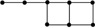
Figure 2: extended domino $H_{4}$

If we restrict chordal bipartite graphs to degree at most 3 then we obtain the following result:

Theorem 7.

Let $G=(X,Y,E)$ be a chordal bipartite graph with vertex degree at most $3$. Then:

• $G^{2}$ is hole-free.

• If $G$ is $H_{4}$-free then $G^{2}$ is $A_{4}$-free.

Proof. $(i)$: Suppose to the contrary that there is a hole $(v_{1},\ldots,v_{k})$, $k\geq 5$, in $G^{2}$. Without loss of generality, let $v_{1}\in X$. If $d_{G}(v_{i},v_{i+1})=2$ (modulo $k$) for all $i\in\{1,\ldots,k\}$ then all common neighbors of $v_{i},v_{i+1}$ are in $Y$ and thus, there is a hole in $G$, which is a contradiction since $G$ is chordal bipartite. Thus, at least one of the pairs $v_{i},v_{i+1}$ has distance 1; without loss of generality let $v_{1}v_{2}\in E$. Then $d_{G}(v_{k},v_{1})=2$ and $d_{G}(v_{2},v_{3})=2$; let $x_{2}\in X$ be a common neighbor of $v_{2},v_{3}$ and let $y_{k}\in Y$ be a common neighbor of $v_{k},v_{1}$. If $x_{2}y_{k}\notin E$ then it leads to a hole in $G$ which is impossible. Thus, $x_{2}y_{k}\in E$ but now, the degrees of $x_{2}$ and $y_{k}$ are 3, and thus, by the degree bound, $x_{2}$ and $y_{k}$ have no other neighbors. Now the cycle $(x_{2},v_{3},\ldots,v_{k},y_{k})$ leads to a hole in $G$, which is a contradiction. Thus, $G^{2}$ is hole-free.

$(ii)$: Suppose to the contrary that $v_{1},\ldots,v_{5}$ induce an $A_{4}$ in $G^{2}$ with $C_{4}$ $(v_{1},v_{2},v_{3},v_{4})$ in $G^{2}$ and vertex $v_{5}$ with $v_{5}v_{3}\in E(G^{2})$ such that $v_{5}$ is nonadjacent to $v_{1},v_{2},v_{4}$ in $G^{2}$. If the pairwise distance of $v_{i},v_{i+1}$ is 2 for every $i\in\{1,2,3,4\}$ (modulo 4) then it forms a hole in $G$. Thus, assume that $d_{G}(v_{1},v_{4})=1$; let $v_{1}\in X$ and $v_{4}\in Y$. Then, as above, $d_{G}(v_{1},v_{2})=2$ (since $v_{2}v_{4}\notin E(G^{2})$) and $d_{G}(v_{3},v_{4})=2$ (since $v_{1}v_{3}\notin E(G^{2})$). Thus, $v_{2}\in X$ and $v_{3}\in Y$, and now $d_{G}(v_{2},v_{3})=1$. Let $y_{1}\in Y$ be a common neighbor of $v_{1},v_{2}$, and let $x_{3}\in X$ be a common neighbor of $v_{3},v_{4}$. Since $G$ is hole-free, $y_{1}x_{3}\in E$. Then $d_{G}(v_{3},v_{5})=2$ since $v_{2}v_{5}\notin E(G^{2})$, i.e., $d_{G}(v_{2},v_{5})\geq 3$; let $x_{5}\in X$ be a common neighbor of $v_{3},v_{5}$. By the degree bound and since $deg_{G}(y_{1})=3$, we have $y_{1}x_{5}\notin E$. Then, $v_{1},\ldots,v_{5},y_{1},x_{3},x_{5}$ induce an $H_{4}$ (as shown in Figure 2), which is a contradiction.

Thus, Theorem 7 is shown. ∎

Corollary 5.

For $H_{4}$-free chordal bipartite graphs with vertex degree at most $3$, ED is solvable in polynomial time.

Recall that ED is $\mathbb{NP}$-complete for bipartite graphs of vertex degree at most 3 [16] and girth at least $g$ for every fixed $g$ [33].

Theorem 8.

For $P_{9}$-free bipartite graphs with vertex degree at most $3$, ED is solvable in polynomial time.

Proof. Let $G=(V,E)$ be a $P_{9}$-free bipartite graph with vertex degree at most $3$. Again, by Theorem 2 and by the e.d.s. property, when checking whether $v\in V$ is part of an e.d.s. $D$ of $G$, we can assume that its distance levels $N_{k}$, $k\geq 6$, are empty. By Claim 2.3 $(iii)$ and (2), we can assume that every vertex in $N_{3}$ has a neighbor in $N_{4}$. We first show:

Claim 3.1.

$|D\cap N_{3}|\leq 2$.

Proof. Suppose to the contrary that $|D\cap N_{3}|\geq 3$; let $y_{1},y_{2},y_{3}\in D\cap N_{3}$, and let $z_{i}$, $i\in\{1,2,3\}$ be neighbors of $y_{i}$ in $N_{4}$ and let $x_{i}$, $i\in\{1,2,3\}$ be neighbors of $y_{i}$ in $N_{2}$. Clearly, by the e.d.s. property and by (3), $x_{1},y_{1},z_{1},x_{2},y_{2},z_{2},x_{3},y_{3},z_{3}$ induce a $3P_{3}$ in $G$. Let $u_{i}\in N_{1}$, $i\in\{1,2,3\}$, be a common neighbor of $v$ and $x_{i}$. By the degree bound 3, there is no common neighbor $u\in N_{1}$ of $x_{1},x_{2}$, and $x_{3}$.

First assume that for two of $x_{1},x_{2},x_{3}$, there is a common neighbor in $N_{1}$; without loss of generality, let $u_{1}x_{1}\in E$ and $u_{1}x_{2}\in E$ for $u_{1}\in N_{1}$. Then, by the degree bound 3, $u_{1}x_{3}\notin E$, and thus, there is a distinct neighbor $u_{3}\in N_{1}$ with $u_{3}x_{3}\in E$. Since $z_{1},y_{1},x_{1},u_{1},v,u_{3},x_{3},y_{3},z_{3}$ do not induce a $P_{9}$ in $G$, we have $u_{3}x_{1}\in E$, and since $z_{2},y_{2},x_{2},u_{1},v,u_{3},x_{3},y_{3},z_{3}$ do not induce a $P_{9}$ in $G$, we have $u_{3}x_{2}\in E$, which is a contradiction to the degree bound 3. Thus, there is no common neighbor in $N_{1}$ of two of the vertices $x_{1},x_{2},x_{3}$; each of $x_{i}$ has its private neighbor $u_{i}\in N_{1}$, $i\in\{1,2,3\}$. But then $z_{1},y_{1},x_{1},u_{1},v,u_{2},x_{2},y_{2},z_{2}$ induce a $P_{9}$ in $G$, which is a contradiction. Thus $|D\cap N_{3}|\leq 2$. $\diamond$

Thus, for every pair $y_{1},y_{2}\in N_{3}$, we can check whether there is an e.d.s. $D$ of $G$ with $v,y_{1},y_{2}\in D$ by reducing the graph correspondingly; let $N^{\prime}_{4}:=N_{4}\setminus(N(y_{1})\cup N(y_{2}))$. Again, we can assume that all vertices in $N^{\prime}_{4}$ have a neighbor in $N_{5}$ since otherwise, such vertices are $(v,y_{1},y_{2})$-forced by the assumption that $v,y_{1},y_{2}\in D$. By similar arguments as for Claim 3.1, we can show that $|D\cap N_{4}|\leq 2$ and finally, for vertices $z_{1},z_{2}\in N^{\prime}_{4}\cap D$, $N_{5}\setminus(N(z_{1})\cup N(z_{2}))\subset D$ is forced. Thus, Theorem 8 is shown. ∎

By the degree bound 3, it is obvious that a bipartite graph $G$ with induced subgraph $K_{3,3}$ has no e.d.s. Moreover, for a $K_{2,3}$ with degree 3 vertices $a$ and $b$, these two vertices are excluded. What is the complexity of ED for $K_{2,3}$-free bipartite graphs with vertex degree at most 3?

4 $\mathbb{NP}$-completeness of ED for some subclasses of bipartite graphs

In [1], it is shown that ED is $\mathbb{NP}$-complete for graphs with diameter at most 3. For bipartite graphs we show:

Theorem 9.

ED is $\mathbb{NP}$-complete for bipartite graphs with diameter at most $6$.

Proof. The proof is based on the transformation from the Exact Cover problem X3C to ED for bipartite graphs. Let $H=(V,{\cal E})$ with $V=\{v_{1},\ldots,v_{n}\}$ and ${\cal E}=\{e_{1},\ldots,e_{m}\}$ be a hypergraph with $|e_{i}|=3$ for all $i\in\{1,\ldots,m\}$. Let $G_{H}$ be the following transformation graph:

$V(G_{H})=V\cup X\cup Y\cup\{z,w,u\}$ such that $X=\{x_{1},\ldots,x_{m}\}$, $Y=\{y_{1},\ldots,y_{m}\}$ and $V,X,Y,\{z,w,u\}$ are pairwise disjoint. The edge set $E(G_{H})$ of $G_{H}$ consists of the following edges: First, $v_{i}x_{j}\in E(G_{H})$ whenever $v_{i}\in e_{j}$. Moreover $V$ is an independent set in $G_{H}$, every $y_{i}$ is only adjacent to $x_{i}$ in $G_{H}$, $z\text{{\footnotesize1}⃝}V$, and $zw,wu\in E(G_{H})$.

Clearly, $G_{H}$ is bipartite, and it is easy to see that the diameter of $G_{H}$ is at most $6$.

Next we show that $H=(V,{\cal E})$ has an exact cover if and only if $G_{H}$ has an e.d.s. $D$:

For an exact cover ${\cal E}^{\prime}\subset{\cal E}$ of $H$, every $e_{i}\in{\cal E}^{\prime}$ corresponds to vertex $x_{i}\in D$, and every $e_{i}\notin{\cal E}^{\prime}$ corresponds to vertex $y_{i}\in D$. Moreover, $w\in D$. Thus, $D$ is an e.d.s. of $G_{H}$.

Conversely, if $D$ is an e.d.s. in $G_{H}$ then $V\cap D=\emptyset$ since otherwise, by the e.d.s. property, some $y_{i}$ cannot be dominated. Analogously, $z\notin D$ since otherwise, $u$ cannot be dominated. Thus, $w\in D$ is forced, and now, $D\cap X$ corresponds to an exact cover of $H$, namely for $D=\{x_{i_{1}},\ldots,x_{i_{k}}\}$, $\{N(x_{i_{1}})\cap V,\ldots,N(x_{i_{k}})\cap V\}$ is an exact cover of $H$. ∎

This proof can be easily extended for showing that ED is $\mathbb{NP}$-complete for $C_{4}$-free bipartite graphs (and more generally, for $(C_{4},C_{6},\ldots,C_{2k})$-free bipartite graphs for every fixed $k\geq 3$): As a first step, every edge $x_{i}v_{j}\in E(G_{H})$ has to be replaced by a $P_{5}$ $P(x_{i},v_{j})$ with end-vertices $x_{i}$ and $v_{j}$ and private internal vertices. Let $P(x_{i},v_{j})=(x_{i},a,b,c,v_{j})$. If $x_{i}\in D$ then $c\in D$ is forced, and if $x_{i}\notin D$ then $b\in D$ is forced. Clearly, the replacement of $G_{H}$ is $C_{4}$-free, and iteratively, the replacement is $(C_{4},C_{6},\ldots,C_{2k})$-free).

The result of Nevries [33] that ED is $\mathbb{NP}$-complete for planar bipartite graphs with degree 3 and girth at least $g$ has been mentioned already but the special case of $(C_{4},C_{6},\ldots,C_{2k})$-free bipartite graphs mentioned above is much easier to prove (clearly, the iterative replacement of $G_{H}$ is not planar bipartite and does not have vertex degree 3 but has girth at least $g$).

5 Conclusion

Open problems: What is the complexity of ED for $P_{k}$-free bipartite graphs, $k\geq 8$, for $S_{1,3,3}$-free bipartite graphs, for $S_{1,1,5}$-free bipartite graphs, and in general for $S_{2,2,k}$-free bipartite graphs for $k\geq 5$, and for chordal bipartite graphs with vertex degree at most $3$?

Acknowledgment. The second author would like to witness that he just tries to pray a lot and is not able to do anything without that - ad laudem Domini.

References

- [1] G. Abrishami and F. Rahbarnia, Polynomial time algorithm for weighted efficient domination problem on diameter 3 planar graphs, Information Processing Letters 140 (2018) 25-29.
- [2] V.E. Alekseev, On the number of maximal stable sets in graphs from hereditary classes, in: Combinatorial Algebraic Methods in Discrete Optimization, University of Nishny Nowgorod, 1991, pp. 5-8 (in Russian).
- [3] G. Bacsó and Zs. Tuza, A characterization of graphs without long induced paths, J. Graph Theory 14, 4 (1990) 455-464.
- [4] E. Balas and Ch.S. Yu, On graphs with polynomially solvable maximum-weight clique problem, Networks 19 (1989) 247-253.
- [5] D.W. Bange, A.E. Barkauskas, and P.J. Slater, Efficient dominating sets in graphs, in: R.D. Ringeisen and F.S. Roberts, eds., Applications of Discrete Math. (SIAM, Philadelphia, 1988) 189-199.
- [6] D.W. Bange, A.E. Barkauskas, L.H. Host, and P.J. Slater, Generalized domination and efficient domination in graphs, Discrete Math. 159 (1996) 1-11.
- [7] N. Biggs, Perfect codes in graphs, J. of Combinatorial Theory (B), 15 (1973) 289-296.
- [8] A. Berry, A. Brandstädt, and K. Engel, The Dilworth number of auto-chordal bipartite graphs, Graphs and Combinatorics 31 (2015) 1463-1471.
- [9] A. Brandstädt, Efficient Domination and Efficient Edge Domination: A Brief Survey, in: B.S. Panda and P.S. Goswami (Eds.), CALDAM 2018, LNCS 10743, pp. 1-14, 2018.
- [10] A. Brandstädt, P. Fičur, A. Leitert, and M. Milanič, Polynomial-time algorithms for Weighted Efficient Domination problems in AT-free graphs and dually chordal graphs, Information Processing Letters 115 (2015) 256-262.
- [11] A. Brandstädt and V. Giakoumakis, Weighted Efficient Domination for -Free Graphs in Polynomial Time, CoRR arXiv:1407.4593, 2014.
- [12] A. Brandstädt, V. Giakoumakis, and M. Milanič, Weighted Efficient Domination for some classes of -free and of -free graphs, Discrete Applied Math. 250 (2018) 130-144.
- [13] A. Brandstädt, A. Leitert, and D. Rautenbach, Efficient Dominating and Edge Dominating Sets for Graphs and Hypergraphs, extended abstract in: Conference Proceedings of ISAAC 2012, LNCS 7676, 2012, 267-277. Full version: CoRR, arXiv:1207.0953v2, [cs.DM], 2012.
- [14] A. Brandstädt, V.B. Le, and J.P. Spinrad, Graph Classes: A Survey, SIAM Monographs on Discrete Math. Appl., Vol. 3, SIAM, Philadelphia (1999).
- [15] A. Brandstädt, V.V. Lozin, and R. Mosca, Independent Sets of Maximum Weight in Apple-Free Graphs, SIAM J. Discrete Math. 24, 1 (2010) 239-254.
- [16] A. Brandstädt, M. Milanič, and R. Nevries, New polynomial cases of the weighted efficient domination problem, extended abstract in: Conference Proceedings of MFCS 2013, LNCS 8087, 195-206. Full version: CoRR arXiv:1304.6255, 2013.
- [17] A. Brandstädt and R. Mosca, Weighted efficient domination for -free and -free graphs, extended abstract in: Proceedings of WG 2016, P. Heggernes, ed., LNCS 9941, pp. 38-49, 2016. Full version: SIAM J. Discrete Math. 30, 4 (2016) 2288-2303.
- [18] B. Courcelle, J.A. Makowsky, and U. Rotics, Linear time solvable optimization problems on graphs of bounded clique-width, Theory of Computing Systems 33 (2000) 125-150.
- [19] K. Dabrowski, V.V. Lozin, and V. Zamaraev, On factorial properties of chordal bipartite graphs, Discrete Math. 312 (2012) 2457-2465.
- [20] K. Dabrowski and D. Paulusma, Classifying the clique-width of -free bipartite graphs, Discrete Applied Math. 200 (2016) 43-51.
- [21] M. Farber, On diameters and radii of bridged graphs, Discrete Math. 73 (1989) 249-260.
- [22] M. Farber, M. Hujter, and Zs. Tuza, An upper bound on the number of cliques in a graph, Networks 23 (1993) 75-83.
- [23] M.R. Garey and D.S. Johnson, Computers and Intractability–A Guide to the Theory of NP-Completeness, Freeman, San Francisco, 1979.
- [24] R.M. Karp, Reducibility among combinatorial problems, In: Complexity of Computer Computations, Plenum Press, New York (1972) 85-103.
- [25] E. Köhler, Graphs without asteroidal triples, Ph.D. thesis, TU Berlin, 1999.
- [26] V.V. Lozin, Bipartite graphs without a skew star, Discrete Math. 257 (2002) 83-100.
- [27] V.V. Lozin and D. Rautenbach, Chordal bipartite graphs of bounded tree- and clique-width, Discrete Math. 283 (2004) 151-158.
- [28] V.V. Lozin and D. Rautenbach, The tree- and clique-width of bipartite graphs in special classes, Australasian J. Combinatorics 34 (2006) 57-67.
- [29] V.V. Lozin and J. Volz, The clique-width of bipartite graphs in monogenic classes, Rutcor Research Report RRR 31-2006.
- [30] C.L. Lu and C.Y. Tang, Solving the weighted efficient edge domination problem on bipartite permutation graphs, Discrete Applied Math. 87 (1998) 203-211.
- [31] C.L. Lu and C.Y. Tang, Weighted efficient domination problem on some perfect graphs, Discrete Applied Math. 117 (2002) 163-182.
- [32] M. Milanič, Hereditary Efficiently Dominatable Graphs, Journal of Graph Theory 73 (2013) 400-424.
- [33] R. Nevries, Efficient Domination and Polarity, Ph.D. Thesis, University of Rostock, 2014.
- [34] M. Paull and S. Unger, Minimizing the number of states in incompletely specified sequential switching functions, IRE Transactions on Electronic Computers 8 (1959) 356-367.
- [35] E. Prisner, Graphs with few cliques, Graph Theory, Combinatorics and Algorithms, Kalamazoo, MI, 1992, 945-956, Wiley, New York, 1995.