Experimental device-independent tests of quantum channels

Abstract

Quantum tomography is currently the mainly employed method to assess the information of a system and therefore plays a fundamental role when trying to characterize the action of a particular channel. Nonetheless, quantum tomography requires the trust that the devices used in the laboratory perform state generation and measurements correctly. This work is based on the theoretical framework for the device-independent inference of quantum channels that was recently developed and experimentally implemented with superconducting qubits in [Dall’Arno, Buscemi, Vedral, arXiv:1805.01159] and [Dall’Arno, Brandsen, Buscemi, PRSA 473, 20160721 (2017)]. Here, we present a complete experimental test on a photonic setup of two device-independent quantum channels falsification and characterization protocols to analyze, validate, and enhance the results obtained by conventional quantum process tomography. This framework has fundamental implications in quantum information processing and may also lead to the development of new methods removing the assumptions typically taken for granted in all the previous protocols.

Measurements are essential to acquire information about physical systems and its dynamics in any experimental science. In quantum physics, in particular, the importance of measurements is promoted even further since they perturb the quantum system under scrutiny and thus require a new understanding of how to connect observed empirical data with the underlying quantum description of nature. To cope with that, we can rely on quantum tomography tomo1 ; tomo2 ; tomo3 , a general procedure to reconstruct quantum states and channels from the statistics obtained by measurements on ensembles of quantum systems. However, how can one guarantee that the measurement apparatus is measuring what it is supposed to? In practice, experimental errors are unavoidable and such deviations from an ideal scenario not only can lead to the reconstruction of unphysical states unph but also imply false positives in entanglement detection ent1 ; ent2 ; ent3 and compromise the security in quantum cryptography protocols cryp1 ; cryp2 ; cryp0 ; cryp00 .

Strikingly, with the emergence of quantum information science, a new paradigm has been established for the processing of information. This is the so-called Device-Independent (di) approach div ; dient ; div2 ; Dal17 ; DBBV17 , a framework where conclusions and hypotheses about the system of interest can be established without the need of a precise knowledge of the measurement apparatus/devices. The prototypical example of how the di reasoning works is given by Bell’s theorem Bell1 ; Bell2 , which implies experimentally testable inequalities, whose violation certifies the presence of entanglement and provides further information about the quantum state, such as its dimension dim1 ; dim2 or fidelity with a maximally entangled state div3 . In other words, even with no information whatsoever about what measurements are being performed, general features of the quantum state can be recovered. A natural question is then whether the di approach can also be adopted within the other pillar of quantum tomography: the reconstruction of quantum channels.

Figure 1: Schematic representation of a measurement process. A state $\rho_{i}$ is prepared and sent through the unknown channel, after which we perform a measurement $\pi_{j}$. Repeating the process for different combinations of states and measurements we get the correlations $p_{j|i}$.

This question was very recently answered on the affirmative by Dall’Arno et al. in Refs. dell2018 ; ditest , where a theoretical framework for the device-independent inference of unknown quantum channels, given as a black-box, was derived and experimentally implemented with superconducting qubits. In this article, we adopt the theoretical tools developed in dell2018 ; ditest and implement a di validation test of a quantum process tomography, i.e. device-independent tomography validation (di-tv). This protocol is schematically represented in Fig.2a and can be adopted after a usual tomography has been performed on a given quantum channel, in order to falsify or validate the channel reconstruction obtained from the data. As a further step, we propose an algorithm to provide a confidence range within which the tomography is validated (see also dell2018 for the discussion of a different algorithm for the same purpose). Following the di-tv, we implement a second protocol, depicted in Fig.2b: a device-independent channel characterization (di-cc), where we have no information about the nature of the channel and, by preparing random quantum states and measuring random observables, we can determine the quantum channel equivalence class that is the most compatible with the measurement data. The two protocols, recently introduced in dell2018 are applied here on two different types of quantum channels, the amplitude damping and the dephased amplitude damping channels, by exploiting a photonic setup and using a qubit encoded in the polarization degree of freedom.

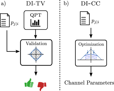
Figure 2: Summary of the DI tests. di-tv (device-independent tomography validation): We first perform a standard quantum process tomography (QPT) on the channel, using maximum likelihood estimation likel ; hrad . We then find the set of correlations compatible with the reconstructed channel and perform additional measurements, obtaining correlations $p_{j|i}$ that can invalidate the QPT if they do not belong to the expected set. b) di-cc (device-independent channel characterization): In this case we do not perform the QPT, instead we collect a fixed number of correlations $p_{j|i}$, spanning uniformly the Bloch sphere with the states $\rho_{i}$ and measurements $\pi_{j}$ (but, as opposed to QPT, without any assumption on their actual physical implementation). Then we find the channel parameters (see  dell2018 ; ditest and Supplementary Material) that best fit the set of experimentally found correlations.

The scenario of interest is depicted in Fig. 1. In order to characterize an unknown quantum channel $\mathcal{X}$ via tomography, we prepare a number of known quantum states $\rho_{i}$ that evolve as $\mathcal{X}(\rho_{i})$ and that are then measured according to a measurement operator $\pi_{j}$ associated with outcome $j$. For example, for a single qubit, quantum process tomography (QPT) qpt1 requires the preparation of the states $\ket{0}$, $\ket{1}$, $\ket{+}=(\ket{0}+\ket{1})/\sqrt{2}$, $\ket{R}=(\ket{0}-i\ket{1})/\sqrt{2}$ and the projection onto the eigenstates of the Pauli matrices $\sigma_{x}$, $\sigma_{y}$ and $\sigma_{z}$. By the Born’s rule we associate the observed statistics with the state and measurements via $p_{j|i}=\mathrm{Tr}\left[\pi_{j}\mathcal{X}(\rho_{i})\right]$ and, if we know $\rho_{i}$ and $\pi_{j}$, this equation can be inverted to find the expression for the channel $\mathcal{X}$. However, if we have no information (or trust) about the states and measurements, what kind of relevant information can be extracted from the observed statistics $p_{j|i}$? As proposed in ditest ; dell2018 , a given quantum channel defines a convex set of correlations $p_{j|i}$ that are compatible with it. Thus, if the experiment produces a point $p_{j|i}$ outside the boundary of the correlation set of a channel, taken as hypothesis (for example arising from the quantum process tomography), we can unambiguously exclude this channel as potential candidate for our reconstruction. Alternatively, if the measured correlation points $p_{j|i}$ fall within the set, the hypothesis is not falsified and one can move further, searching for a confidence level within which the quantum process tomography prediction is validated. Moreover, overlooking any device-dependent channel reconstruction, one can find the best quantum channel fitting the data, as the “minimal surviving hypothesis”, that is, the channel $\mathcal{X}^{*}$ whose boundary contains all the observed correlations set, but minimizing the surrounded volume dell2018 . Note that this protocol cannot unambiguously determine all of the characterizing parameters of the quantum channel, so it actually enables to single out the equivalence class to which it belongs (see Supplementary Material of dell2018 ). Considering the case where $i,j=0,1$, that is two possible state preparations and a dichotomic measurement, analytical expressions characterizing a large class of qubit channels, which are invariant under the dihedral group $D_{2}$, have been obtained ditest ; dell2018 . This class of channels can be represented by four real numbers $\left(d_{1},d_{2},d_{3},c_{3}\right)$ and maps the Bloch sphere into an ellipsoid translated along one of its own axis. This transformation is pictorially represented in Fig. 3 (see Supplementary Material for further details), which shows that geometrically $d_{1}$, $d_{2}$ and $d_{3}$ represent the ellipsoid’s axes, and $c_{3}$ the translation along the $z$ axis.

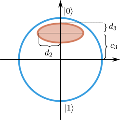
Figure 3: Bloch-sphere representation of the action of a general qubit dihedrally-covariant channel. The Bloch-sphere is mapped into an ellipsoid with semi-axis $d_{1}$, $d_{2}$, and $d_{3}$, which is translated along one of its own axis ($d_{3}$, in the figure) by a distance $c_{3}$.

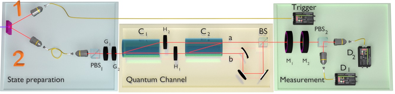
Figure 4: Experimental apparatus. In the preparation stage a couple of photons is generated by a spontaneous parametric down-conversion (SPDC) process in a non-linear crystal. Photon 1 will act as a trigger while photon 2’s polarization encodes the particular qubit to be analyzed. The state preparation is performed by a polarizing beam splitter (PBS₁), a quarter-wave plate ($G_{1}$) and a half-wave plate ($G_{2}$), which rotates the horizontal polarization of incoming photons in order to generate $\sqrt[]{\omega}\ket{0}$+$\sqrt[]{1-\omega}\ket{1}$. After the preparation of the state, photon 2 is sent to the amplitude damping channel section (yellow stage) composed by a first calcite crystal ($C_{1}$), two half-wave plates ($H_{1}$ and $H_{2}$) one for each generated path and another calcite crystal ($C_{2}$) to recombine the paths. Setting the angle of $H_{1}$ at $45^{o}$ we are able to close the calcite interferometer thus sending the photons to the output “a”. Conversely, when $H_{1}$ is at $0^{o}$, photon 2 comes out in path “b” projected onto the vertical polarization $\ket{V}$. The two paths “a” and “b” are incoherently recombined at the beam splitter (BS). Intermediate angles between $0^{o}$ and $45^{o}$ for $H_{2}$ and $H_{1}$ allow to tune the contribution $\ket{H}$ and $\ket{V}$ to be recombined in the BS. The measurement stage is composed by a quarter-wave plate ($M_{1}$), a half-wave plate ($M_{2}$) and a PBS, after which the photons are coupled into single-mode (SM) fibers connected to single photon detectors.

Device-independent tomography validation– Now, let us consider the goal to characterize an implemented quantum channel through a tomography, but not trusting our apparatus and therefore requiring a device-independent validation to state its correct functioning. Sticking to the hypothesis of $D_{2}$ covariance, we perform the QPT, restricting to the hypothesis of dihedral covariance (see Supplementary Material), and find the four parameters ($d_{1}$, $d_{2}$, $d_{3}$, $c_{3}$) that identify our channel. This restriction is fully supported by our experimental evidence, indeed the fidelity between the general and the $D_{2}$ covariance restricted quantum process tomographies, performed on all the implemented channels, has been found to be always higher than 0.99. As following step, we are able to reconstruct the hypothetical channel’s boundary of the set of input/output correlations ditest ; dell2018 . The tomographic experiment is device-independently proved to be trustworthy if, uniformly spanning the whole set of correlations, all the observed data fall within the boundary. Otherwise, the quantum process tomography is falsified. In principle, it is possible to exploit the same data set, both for the quantum process tomography and the DI validation. Indeed, in the latter case, the data would be interpreted as bare correlations, without any assumptions about states and measurements. Clearly, however, a better validation includes additional experimental data probing the boundary of the set defined by the channel being validated. After a tomographic reconstruction is validated, we need to quantify the quality of our tomographic reconstruction, since, if the boundary lies too far from the observed points, the hypothesis, although in principle validated, would not be really supported by the data. In other words, a good hypothesis is an “almost falsified one”: its boundaries should enclose all the observed correlations, but not much more dell2018 .

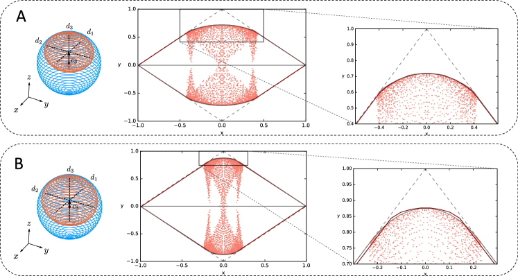
Figure 5: Device Independent Test of a Quantum Process Tomography. From a QPT on two channels, imposing $D_{2}$ covariance, we evaluate the four characteristic parameters ($d_{1}$, $d_{2}$, $d_{3}$ and $c_{3}$). The action of the channels on the Bloch sphere is shown on the left, where the orange ellipsoid represents the deformation of the original unit sphere, in blue. The correlations set is surrounded by the red curve. To certificate the QPT, we feed our channel with orthogonal pure states belonging to the XZ plane of the Bloch sphere. In order to cover a significant part of the correlations set, we test all possible combinations of states and measurements. The blank corners within the curves, which are trivial for our analysis (can be obtained by a convex combination of the other points), are not covered, since the channel was fed only with orthogonal states and only orthogonal projection measurements were performed.

	($d_{1}$, $d_{2}$, $d_{3}$, $c_{3}$)	Parameters’ variation range	$\Delta$	$\mu$
A	(0.719, 0.791, 0.596, 0.397)	(-, -), (-0.025, +0.051), (-0.038, +0.023), (-0.028, +0.034)	0.004	0.692
B	(0.815, 0.877, 0.791, 0.231)	(-, -), (-0.010, +0.020), (-0.025, +0.014), (-0.012, +0.029)	0.005	0.763

Table 1: Device-Independent Tomography Validation. Characteristic parameters ($d_{1}$, $d_{2}$, $d_{3}$, $c_{3}$) obtained for the two channels A and B. The confidence level indicators given by tomography validation are in the right two columns: the parameters’ variation range within which the QPT would still be validated, and the $\Delta$, which quantifies the relative difference between the two area of the correlations sets. In the last column on the right we report the $\mu$ parameters, which define the equivalence class to which each of the two channels belongs.

This protocol was applied to experimental data, in order to validate quantum process tomography on 1-qubit quantum channels. The implementation, as well as the characterization of the channels, was performed exploiting the photonic platform in Fig.4. The setup can be seen as made of three parts: (i) photonic state preparation, (ii) quantum channel, (iii) measurement station. In part (i), the desired state is prepared encoding one qubit in the polarization degree of freedom of a photon which goes through an apparatus made of a polarizing beam splitter ($PBS_{1}$), followed by a quarter- and half- wave plate ($G_{1}$ and $G_{2}$). The photon is generated by a heralded photon source making use of a spontaneous parametric down-conversion (SPDC) process, where the second photon of the pair is used as a trigger. In part (ii), our quantum channel is made of two birefringent calcite crystals ($C_{1}$ and $C_{2}$), followed by a beam splitter, and has the aim of introducing a desired amount $\lambda$ of decoherence between path a and b, depending on the rotation of the half-wave plate $H_{2}$. The measurement station in part (iii) allows to perform projective measurements, through the sequence of a quarter- and a half- wave plate ($M_{1}$ and $M_{2}$), followed by a $PBS_{2}$ (see Supplementary Material).

By exploiting the aforementioned apparatus, we implemented an amplitude damping channel $\mathcal{X}^{\mathrm{AD}}$ acting as

$$\mathcal{A}_{\lambda}(\rho)\mathrel{\mathop{\mathchar 58\relax}}=A_{0}\rho A_{0}^{\dagger}+A_{1}\rho A_{1}^{\dagger},\quad\begin{cases}A_{0}=\ket{0}\!\!\bra{0}+\sqrt{1-\lambda}\ket{1}\!\!\bra{1},\\ A_{1}=\sqrt{\lambda}\ket{0}\!\!\bra{1},\end{cases}$$

with varying efficiency (i.e. the amount of noise) of the channel as quantified by a parameter $\lambda$. First, we performed a QPT over this channel, whose estimated action on the Bloch sphere is depicted in orange, in Fig. 5a and Fig. 5b. The noise corresponds to deformations of the Bloch sphere: the size of the orange ellipsoid is inversely proportional to the noise strength $\lambda$. Through the QPT, we evaluated the four characteristic parameters ($d_{1},d_{2},d_{3},c_{3}$), reported in Tab.1. Using the results in ditest ; dell2018 we could then compute the boundary of the set of input/output correlations and the states and measurements allowing us to probe this boundary (see Supplementary Material). To validate the QPT hypothesis, we prepared 29 different pairs of orthogonal states and projected each of these couples onto 29 pairs of orthogonal directions, in order to span a significant part of correlations set, using in total 841 combinations of states and measurements for each plot.

Both tomographies were validated, since, within 2$\sigma$, all the points lie inside the boundary, as it is shown in the plots in Fig.5a,b. The confidence level was estimated in two ways. First, as proposed in dell2018 , by evaluating the relative difference between the union and the intersection of the two correlation sets ($\Delta$). The obtained values were respectively 0.004 (A) and 0.005 (B). A second evaluated quantity was the variation range associated to each of the parameters ($d_{2}$, $d_{3}$, $c_{3}$) for each channel, reported in Tab.1. This is the range of values within which the characterizing parameters would still allow to validate the QPT. This kind of uncertainty was achieved imposing the two following conditions: for every parameter set in the given range, the QPT boundary strictly surrounds all the experimental points (within 1$\sigma$), and the $\Delta$ parameter cannot be larger than 2 times its original value. As mentioned before, our device-independent procedure cannot determine all of the four parameters ($d_{1}$, $d_{2}$, $d_{3}$, $c_{3}$), specifically, it is insensitive to either $d_{1}$ or $d_{2}$ (see dell2018 ). We choose $d_{1}$ as the parameter that the procedure is insensitive to, so its uncertainty is not reported. Adopting this protocol, with no assumptions on the implementation nor on the state generation/measurement execution, we were able to recognize the equivalence class of our channel in a fully device-independent way. Indeed, the device-independent boundary reconstruction can be the same for different quantum channels, as reported in dell2018 . We can, therefore, define the following quantity: $\mu\left(\mathcal{C}_{d_{1},d_{2},d_{3},\vec{c}}\right)=(1-c_{3})(d_{2}^{2}-d_{3}^{2})/(c_{3}d_{3}^{2})$; this parameter specifies the equivalence class to which the reconstructed quantum channel belongs. In our case, for both the implemented quantum channels, $0\leq\mu\leq 1$, as reported in Tab.1. Within this regime, two device independent reconstructions $\mathcal{C}_{(d_{1},d_{2},d_{3},\vec{c})}$ and $\mathcal{C}_{(d^{\prime}_{1},d^{\prime}_{2},d^{\prime}_{3},\vec{c}^{\prime})}$ are indistinguishable when $(d_{2},d_{3},c_{3})=(d_{2}^{\prime},d_{3}^{\prime},c_{3}^{\prime})$. This allows to recognize whether our apparatus is working correctly, generating the correct states and performing the required measurements. As pointed out above, the most plausible hypothesis describing a set of correlations is the one whose boundary encloses all the correlation points while being as close as possible to them.

Device-independent channel characterization The second implemented protocol, the device-independent Channel Characterization (di-cc), naturally arises if the above insight is lifted to the level of a guiding principle to choose the most plausible hypothesis compatible with the observed data, as discussed in Ref. dell2018 . The idea here is to single out the “minimal surviving hypothesis”, that is the channel $\mathcal{X}^{*}$ whose boundary encloses the smallest volume $V(\mathcal{X}^{*})$ in correlation space but still contains all the observed correlations set $\mathcal{D}=\{(x_{k},y_{k})\}$. According to this idea, first introduced in dell2018 , the best candidate channel is given by

$$\mathcal{X}^{*}=\arg\min_{\begin{subarray}{c}\mathcal{X}\ \mathrel{\mathop{\mathchar 58\relax}}\ \mathbb{D}_{2}\\ \mathcal{D}\subseteq\mathcal{S}(\mathcal{X})\end{subarray}}V(\mathcal{X}).$$ (1)

where $\mathcal{S}(\mathcal{X})$ is the set of correlations associated with the channel $\mathcal{X}$. This set can be spanned sending states and performing projections which are uniformly distributed over the Bloch sphere.

In the experiment, we covered a significant part of this set, through 841 pairs of state/measurement combinations, as in the previous case. Here, the aim is to characterize the implemented channel without relying on any device-dependent procedure. After the parametrization of the experimental data, the boundary of the correlation set is obtained through a minimization algorithm, based on sequential quadratic programming slsqp , with the aim of finding the minimum area which contains all the correlation set, compatible with the constraints imposed by the dihedral covariance of the channel (see the Supplementary Material). Exploiting this protocol we can identify, in an entirely device-independent way, the equivalence class to which our channel belongs (see dell2018 ), through three of the four characterizing parameters ($d_{2}$, $d_{3}$, $c_{3}$, again $d_{1}$ is chosen as the parameter that the procedure is insensitive to). This procedure effectively extracts from our measurements as much information as we are allowed to, without assuming anything about the measuring device. We test the di-cc protocol using the experimental setup described in the previous paragraph, setting five different $\lambda$ parameters and also introducing an additional dephasing by carefully tuning the position of the calcite crystals. The results for the $d_{2}$, $d_{3}$, $c_{3}$ parameters of the five different channels are shown in Tab. 2, while in Fig. 6 we show the correlation set, along with the optimal boundary, for channels A, C, D, and E. To evaluate the reliability of this protocol we compare the results with the ones obtained using standard tomographic techniques (see Supplementary Material), using again the relative difference between the union and intersection areas of the correlation sets, which is shown in Tab. 2 as $\Delta$. In Fig. 6, the gray boundaries are those estimated by the QPT on the channels, whose actions on the Bloch sphere is shown on the left side of each plot. The experimental data are shown in purple and the boundaries evaluated through the optimization algorithm are drawn in green. Fig. 6c corresponds to the channel in which the additional dephasing factor is present. There is good agreement between the di-cc’s and the QPT’s boundaries, indeed the $\Delta$ parameters are all below $3\%$.

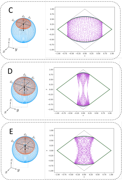
Figure 6: Device Independent Channel Characterization of input-output correlations (DI-CC). Characterization of three channels, implemented with different $\lambda$ parameters. The purple dots are obtained feeding orthogonal pure states belonging to the XZ plane of the Bloch sphere to our channel. The green curves surround the correlations of the di-cc while the blue ones are those obtained by the QPT, imposing $D_{2}$ covariance. For each plot, the action on the Bloch sphere given by the QPT is shown in orange on the left. In the plot the empty sectors can be trivially obtained using non orthogonal states and projectors and are not necessary for our analysis.

	($d_{2}$, $d_{3}$, $c_{3}$)	$\Delta$	$\mu$
A	(0.735, 0.606, 0.394)	0.018	0.723
B	(0.875, 0.789, 0.210)	0.009	0.865
C	(0.612, 0.415, 0.585)	0.027	0.833
D	(0.823, 0.784, 0.215)	0.009	0.372
E	(0.696, 0.675, 0.325)	0.001	0.131

Table 2: Device Independent Channel Characterization. Characteristic parameters ($d_{1}$, $d_{2}$, $d_{3}$, $c_{3}$) with their statistical uncertainties obtained using the di-cc protocol for five different channels A-E. In channel E an artificial dephasing factor was added. In the last column on the right we report the $\mu$ parameters of each device independent channel characterization, which define their equivalence class.

As noted before, the di-cc protocol does not identify the quantum channel unambiguously dell2018 : indeed, for each minimization problem, there is an equivalence class of quantum channels, which optimizes Eq.1, specified by the parameter $\mu$. In this case, all the implemented quantum channels have $0\leq\mu\leq 1$, as reported in Tab.2. This regime, which is the same that was mentioned in the previous paragraph, brings two device independent reconstructions $\mathcal{C}_{(d_{1},d_{2},d_{3},\vec{c})}$ and $\mathcal{C}_{(d^{\prime}_{1},d^{\prime}_{2},d^{\prime}_{3},\vec{c}^{\prime})}$ to be indistinguishable when $(d_{2},d_{3},c_{3})=(d_{2}^{\prime},d_{3}^{\prime},c_{3}^{\prime})$, as proved in dell2018 .

Discussion.– In conclusion, our work provides a strong experimental insight into results recently derived and experimentally implemented with superconducting qubits by Dall’Arno et al. in Refs. dell2018 ; ditest . We apply those results to a photonic implementation, and we introduce an algorithm for the estimation of the confidence level, in addition to that introduced in Ref. dell2018 . Indeed, we apply two device-independent protocols derived in Refs dell2018 ; ditest (device-independent tomography validation, di-tv, and device-independent channel characterization, di-cc) to two types of dihedrally covariant quantum channels (amplitude damping channel and dephased amplitude damping channel), implemented on a photonic platform. These protocols are based only on the set of input/output correlations which can be observed by an experimenter, without the need of trusting the apparatus. Through the aforementioned procedures, we were able to validate the implemented channel reconstruction of a quantum process tomography and to extract the maximum amount of information from the observed correlation set, in a fully device-independent way. This study, therefore, gives new experimental tools which can be adopted to test whether the experimental apparatus is correctly functioning, but free from the vicious cycle affecting device-dependent procedures like QPT, which require the apparatus to be trusted in the preparation of probe states and on the realization of specific projective measurements. The presented protocols do not provide a complete characterization of the implemented quantum channel (that remains undetermined up to its equivalence class), but we believe our results pave the way for future research along this direction.

Acknowledgements.–This work was supported by the ERC-Starting Grant 3D-QUEST (3D-Quantum Integrated Optical Simulation; grant agreement number 307783): http://www.3dquest.eu. RC acknowledges the Brazilian ministries MCTIC, MEC and the CNPq. F.B. was supported by JSPS KAKENHI, grant no. 17K17796. M.D. was supported by the Ministry of Education and the Ministry of Manpower (Singapore).

References

- (1) G. M. D’Ariano, and P. Lo Presti, Quantum tomography for measuring experimentally the matrix elements of an arbitrary quantum operation, Phys. Rev. Lett. 86, 4195 (2001).
- (2) G. M. D’Ariano, M. G. A. Paris and M. F. Sacchi, Quantum tomography, arXiv:quant-ph/0302028 (2003).
- (3) A. I. Lvovsky, Iterative maximum-likelihood reconstruction in quantum homodyne tomography, Journal of Optics B: Quantum and Semiclassical Optics, 6, 6 (2004).
- (4) M. Ziman, M. Plesch, V. Bužek, and P. Štelmachovič, Process reconstruction: From unphysical to physical maps via maximum likelihood, Phys. Rev. A 72, 022106 (2005).
- (5) K. Życzkowski, P. Horodecki, M. Horodecki, and R. Horodecki, Dynamics of quantum entanglement, Phys. Rev. A 65, 012101 (2001).
- (6) R. Horodecki, P. Horodecki, M. Horodecki, and K. Horodecki, Quantum entanglement, Rev. Mod. Phys. 81, 865 (2009).
- (7) O. Gühne, and G. Toth, Entanglement detection, Physics Reports 474, 1-75 (2009).
- (8) N. Gisin, G. Ribordy, W. Tittel, and H. Zbinden, Quantum cryptography, Rev. Mod. Phys 74, 145 (2002).
- (9) C. H. Bennett, F. Bessette, G. Brassard, L. Salvail and J. Smolin, Experimental quantum cryptography, Journal of Cryptology 5, 3-28 (1992).
- (10) D. Deutsch, A. Ekert, R. Jozsa, C. Macchiavello, S. Popescu, and A. Sanpera, Quantum privacy amplification and the security of quantum cryptography over noisy channels, Phys. Rev. Lett. 77, 2818 (1996).
- (11) A. Acin, N. Brunner, N. Gisin, S. Massar, S. Pironio, and V. Scarani, Device-Independent security of quantum cryptography against collective attacks, Phys. Rev. Lett. 98, 230501 (2007).
- (12) R. Gallego, N. Brunner, C. Hadley, and A. Acín, Device-Independent tests of classical and quantum dimensions, Phys. Rev. Lett. 105, 230501 (2010).
- (13) R. Chaves, J. B. Brask and N. Brunner, Device-Independent tests of entropy, Phys. Rev. Lett. 115, 110501 (2015).
- (14) V. D’Ambrosio, F. Bisesto, F. Sciarrino, J. F. Barra, G. Lima, and A. Cabello, Device-Independent certification of high-dimensional quantum systems, Phys. Rev. Lett. 112, 140503 (2014).
- (15) M. Dall’Arno, Device-independent tests of quantum states, arXiv:1702.00575.
- (16) M. Dall’Arno, S. Brandsen, F. Buscemi, and V. Vedral, Device-independent tests of quantum measurements, Phys. Rev. Lett. 118, 250501 (2017).
- (17) J. S. Bell, On the problem of hidden variables in quantum mechanics, Rev. Mod. Phys. 38, 447 (1966).
- (18) J. F. Clauser and A. Shimony, Bell’s theorem. Experimental tests and implications, Reports on Progress in Physics, 41, 12 (1978).
- (19) N. Brunner, S. Pironio, A. Acin, N. Gisin, A. A. Méthot, and V. Scarani, Testing the dimension of Hilbert spaces, Phys. Rev. Lett. 100, 210503 (2008).
- (20) Y.-C. Liang, D. Rosset, J.-D. Bancal, G. Pütz, T. J. Barnea, and N. Gisin, Family of Bell-like inequalities as device-independent witnesses for entanglement depth, Phys. Rev. Lett. 114, 190401 (2015).
- (21) O. Gühne, C.-Y. Lu, W.-B. Gao, and J.-W. Pan, Toolbox for entanglement detection and fidelity estimation, Phys. Rev. A 76, 030305(R) (2007).
- (22) M. Dall’Arno, F. Buscemi, and V. Vedral, Device-Independent Inference of Physical Devices: Theory and Implementation, arXiv:1805.01159 (2018).
- (23) M. Dall’Arno, S. Brandsen, and F. Buscemi, Device-independent tests of quantum channels, Proc. R. Soc. A 473, 20160721 (2017).
- (24) I. L. Chuang and M. A. Nielsen, J., Prescription for experimental determination of the dynamics of a quantum black box, Mod. Opt. 44, 2455 (1997).
- (25) J. B. Altepeter, E. R Jeffrey, and P. G Kwiat, Photonic state tomography, Advances in Atomic, Molecular, and Optical Physics 52, 105-159 (2005).
- (26) Z. Hradil, J. Rehacek, J. Fiurasek and M. Jezek Maximum-Likelihood Methods in Quantum Mechanics in M. Paris, J. Rehacek, Quantum State Estimation, Springer Berlin Heidelberg, 59-112 (2004).
- (27) D. Kraft, Algorithm 733: TOMP–Fortran modules for optimal control calculations, ACM Transactions on Mathematical Software, 20, 3, 262-281 (1994).