Fluctuation-damping of isolated, oscillating Bose-Einstein condensates

Abstract

Experiments on the nonequilibrium dynamics of an isolated Bose-Einstein condensate (BEC) in a magnetic double-well trap exhibit a puzzling divergence: While some show dissipation-free Josephson oscillations, others find strong damping. Such damping in isolated BECs cannot be understood on the level of the coherent Gross-Pitaevskii dynamics. Using the Keldysh functional-integral formalism, we describe the time-dependent system dynamics by means of a multi-mode BEC coupled to fluctuations (single-particle excitations) beyond the Gross-Pitaevskii saddle point. We find that the Josephson oscillations excite an excess of fluctuations when the effective Josephson frequency, $\tilde{\omega}_{J}$, is in resonance with the effective fluctuation energy, $\tilde{\varepsilon}_{m}$, where both, $\tilde{\omega}_{J}$ and $\tilde{\varepsilon}_{m}$, are strongly renormalized with respect to their noninteracting values. Evaluating and using the model parameters for the respective experiments describes quantitatively the presence or absence of damping.

I Introduction

When a system of ultracold, condensed bosons is trapped in a double-well potential with an initial population imbalance, it undergoes Josephson oscillationsSmerzi et al. (1997) between the wells and can, therefore, be referred to as a Bose-Josephson junction (BJJ). Josephson oscillations were observed in a number of experiments.Albiez et al. (2005); Levy et al. (2007); LeBlanc et al. (2011); Spagnolli et al. (2017) Since the experimental systems are almost ideally separated from the environment, a BJJ can serve as a prototype of a nonequilibrium closed quantum system. Because of the unitary time-evolution which prohibits the maximization of entropy, a closed quantum system cannot thermalize as a whole, once driven out of equilibrium. However, strong damping of Josephson oscillations was observed in the experiments by LeBlanc et al.,LeBlanc et al. (2011) whereas the experiments by Albiez et al.Albiez et al. (2005) and by Spagnolli et al. clearly displayed undamped oscillations for extended periods of time. Explaining this discrepancy and, thereby, giving guidelines for designing an experimental setup with or without damping and thermalization, is the aim of this work.

Previously some of the present authors proposed the dynamical heat-bath generation (DBG) as a damping and thermalization mechanism:Posazhennikova et al. (2018, 2016) For a sufficiently complex, isolated quantum system the Hilbert space dimension is so large that only a small subset of the huge amount of quantum numbers characterizing the system’s state vector can be determined in any given experiment. This subset defines a subspace of the total Hilbert space, referred to as the “subsystem” $\mathcal{S}$. Any measurement performed on ${\cal S}$ alone is partially destructive, in that the quantum numbers defining the Hilbert space of ${\cal S}$ are fixed (partial state collapse), but the remaining subspace of undetermined quantum numbers is traced out. This remaining subspace, ${\cal R}$, becomes massively entangledLenk et al. with the states of the subsystem ${\cal S}$ via the many-body dynamics and, hence, acts as a grand-canonical bath or reservoir. By the resulting, effectively grand canonical time evolution of the subsystem $\mathcal{S}$, it will naturally reach a thermal state in the long-time limit,Posazhennikova et al. (2016) if the system is ergodic. Thus, the measurement process itself defines a division into subsystem and reservoir. For instance, when the population imbalance in a BJJ is measured, the Bose-Einstein condensate (BEC) states comprise $\mathcal{S}$, and all the many-body states involving incoherent excitations outside the BEC comprise $\mathcal{R}$. Note that this thermalization process is dynamical and is possible even when the bath states (for a BJJ, the incoherent excitations) are initially not occupied, hence the term dynamical bath generation. By contrast, the so-called eigenstate thermalization hypothesisDeutsch (1991); Srednicki (1994) (ETH) requires the system to be near a many-body eigenstate of the total Hamiltonian (microcanonical ensemble), i.e., it is stationary by construction. See Ref. [Posazhennikova et al., 2018] for a detailed discussion.

The DBG mechanism was corroborated for a BJJ with arbitrary system parameters, where it was shown that incoherent excitations are efficiently generated out of the oscillating BEC due to a parametric resonance.Posazhennikova et al. (2016) The complex thermalization dynamics of a BJJ involving several time scales has been analyzed in detail in Refs. [Posazhennikova et al., 2016, 2018]. In particular, the thermalization time $\tau_{th}$ is necessarily much larger than the BJJ oscillation period, because (1) the incoherent fluctuations are created by the Josephson oscillations themselves and (2) because of the quasi-hydrodynamic long-time dynamics.Posazhennikova et al. (2016)

In the present work we examine this damping mechanism for realistic experimental parameters and specific traps. Previous studies within the two-mode approximationSmerzi et al. (1997); Ananikian and Bergeman (2006); LeBlanc et al. (2011) showed significant, interaction-induced renormalizations of the Josephson frequency, $\tilde{\omega}_{J}$, but did not explain the observed oscillation damping.LeBlanc et al. (2011) A multimode expansion of the Gross-Pitaevskii equation (GPE) in terms of the complete basis of single-particle trap eigenmodes can describe the coherent part of the dynamics in principle exactly. However, the dynamical excitation of higher trap levels also involves the creation of incoherent fluctuations which are not captured by the GPE saddlepoint dynamics. The excitation of higher trap modes and the concatenated creation of incoherent fluctuations is crucial for damping in realistic systems. These fluctuations are captured by the systematic expansion about the GPE saddlepoint (see Sec. II B), involving BEC as well as fluctuation Green’s functions. We find that efficient coupling to higher trap modes occurs if $\tilde{\omega}_{J}$ is in resonance with the excitation energy of one of the trap levels, $\tilde{\omega}_{J}\approx\tilde{\varepsilon}_{m}$, where $\tilde{\omega}_{J}$, as well as $\tilde{\varepsilon}_{m}$, are strongly renormalized and broadened by their mutual coupling and by the interactions. Conversely, in the off-resonant regime, the Josephson oscillations remain undamped over an extended period of time. Our quantitative calculations reveal that the experimental parameters of LeBlanc et al.LeBlanc et al. (2011) are in the strongly damped regime and those of Albiez et al.Albiez et al. (2005) in the undamped regime, in agreement with the experimental findings. This reconciles the apparent discrepancy between these two classes of experiments and supports the validity of the DBG mechanism in Bose-Josephson junctions.

The article is organized as follows. In Sec. II we describe the many-body action used to model the system and its representation in the trap eigenbasis. We develop the nonequilibrium temporal dynamics by means of the Keldysh path integral. Sec. III contains the numerical analysis: the resonance effect responsible for the damping, and a detailed application to the two exemplary experiments, Refs. [Albiez et al., 2005] and [LeBlanc et al., 2011], respectively. This is followed by a discussion and concluding remarks in Sec. IV.

II Formalism

The model for an ultracold gas in a double-well trap potential $V_{\text{ext}}(\mathbf{r})$ with multiple single-particle levels is defined using the functional-integral formalism. It allows for a convenient distinction between the condensate amplitudes in each level, defined by the time-dependent Gross-Pitaevskii saddle point, and the non-condensate excitations. The nonequilibrium dynamics will be described by the functional integral on the Keldysh time contour.

II.1 Multi-mode model

The action $S$ for a trapped, atomic Bose gas with a contact interaction reads in terms of the bosonic fields $\psi(\mathbf{r},t),\psi^{*}(\mathbf{r},t)$,

$$S\left[\psi,\psi^{*}\right] =\int\text{d}^{3}r\text{d}t\,\big{[}\psi^{*}(\mathbf{r},t)G_{0}^{-1}(\mathbf{r},t)\psi(\mathbf{r},t)$$

$$-\frac{\tilde{g}}{2}\psi^{*}(\mathbf{r},t)\psi^{*}(\mathbf{r},t)\psi(\mathbf{r},t)\psi(\mathbf{r},t)\big{]},$$ (1)

where the coupling parameter $\tilde{g}=4\pi\hbar^{2}a_{s}/m$ is proportional to the $s$-wave scattering length $a_{s}$,Vogels et al. (1997); van Kempen et al. (2002) and the inverse free Green function is

$$G_{0}^{-1}(\mathbf{r},t)=\mathrm{i}\partial_{t}-\left(-\frac{\hbar^{2}\nabla^{2}}{2m}+V_{\text{ext}}(\mathbf{r})\right).$$ (2)

The spatial dependence of the field $\psi(\mathbf{r},t)$ may be resolved into the complete, orthonormal basis of single-particle eigenfunctions $\{\varphi_{-}(\mathbf{r}),\varphi_{+}(\mathbf{r}),\varphi_{3}(\mathbf{r}),\varphi_{4}(\mathbf{r}),\,\dots\}$ of the trap,Posazhennikova et al. (2016)

$$\begin{split}\psi(\mathbf{r},t)&=\psi_{+}(\mathbf{r},t)+\psi_{-}(\mathbf{r},t)+\sum_{m=3}^{M}\psi_{m}(\mathbf{r},t)\\ &=\varphi_{+}(\mathbf{r})\phi_{+}(t)+\varphi_{-}(\mathbf{r})\phi_{-}(t)+\sum_{m=3}^{M}\varphi_{m}(\mathbf{r})\phi_{m}(t),\end{split}$$ (3)

with time-dependent amplitudes $\phi_{m}(t)$ and $M$ the number of modes taken into account. The $\varphi_{i}(\mathbf{r})$ are the solutions of the stationary Schrödinger equation with the potential $V_{\text{ext}}(\mathbf{r})$, with eigenfrequencies $\{\varepsilon_{-},\,\varepsilon_{+},\,\varepsilon_{3},\,\varepsilon_{4},\dots\}$. The wavefunctions $\varphi_{-}(\mathbf{r})$ and $\varphi_{+}(\mathbf{r})$ are the two lowest-lying eigenfunctions of $V_{\text{ext}}(\mathbf{r})$ extending over both wells, with odd (-) and even (+) parity, respectively. In view of the anticipated dynamics with different occupation numbers in the two wells, it is useful to define the symmetric and antisymmetric superpositions $\varphi_{1,2}(\mathbf{r})=[\varphi_{-}(\mathbf{r})\pm\varphi_{+}(\mathbf{r})]/\sqrt{2}$, since they are localized in the left or right well, respectively. With the expansion (3) the action takes the form $S=S_{0}+S_{\mathrm{int}}$, with the noninteracting part,

$$S_{0}=\int\text{d}t\left\{\sum_{i=1}^{M}\left[\phi_{i}^{*}\left(\mathrm{i}\partial_{t}-\varepsilon_{i}\right)\phi_{i}\right]-J\left(\phi_{1}^{*}\phi_{2}+\phi_{2}^{*}\phi_{1}\right)\right\},$$ (4)

and the interacting part

$$S_{\text{int}}=-\tfrac{1}{2}\int\text{d}t\sum_{ijkl=1}^{M}U_{ijkl}\,\phi_{i}^{*}(t)\phi_{j}^{*}(t)\phi_{k}(t)\phi_{l}(t),$$ (5)

where the $\phi_{1,\,2}$ are the symmetric and antisymmetric superpositions of the time-dependent fields $\phi_{\pm}(t)$. In this mode representation, the spatial dependence of the Bose field $\psi(\mathbf{r},t)$ is absorbed into the overlap integrals $\varepsilon_{i}$, $J$, and $U_{ijkl}$, which are given by

$$\varepsilon_{i}= \int\text{d}^{3}r\,\varphi_{i}^{*}(\mathbf{r})\,\left(-\frac{\hbar^{2}\nabla^{2}}{2m}+V_{\text{ext}}(\mathbf{r})\right)\,\varphi_{i}(\mathbf{r}),\ \ \$$ (6)

$$\varepsilon_{1}= \,\varepsilon_{2}=\tfrac{1}{2}(\varepsilon_{-}+\varepsilon_{+}),$$ (7)

$$J= \int\text{d}^{3}r\,\varphi_{1}^{*}(\mathbf{r})\,\left(-\frac{\hbar^{2}\nabla^{2}}{2m}+V_{\text{ext}}(\mathbf{r})\right)\,\varphi_{2}(\mathbf{r})$$

$$= \tfrac{1}{2}(\varepsilon_{-}-\varepsilon_{+}),$$ (8)

$$U_{ijkl}= \tilde{g}\int\text{d}^{3}r\,\varphi_{i}^{*}(\mathbf{r})\varphi_{j}^{*}(\mathbf{r})\varphi_{k}(\mathbf{r})\varphi_{l}(\mathbf{r}),$$ (9)

where the bound-state functions $\varphi_{i}(\mathbf{r})$ may be chosen real. Note that a bare Josephson coupling $J$ exists only between the two lowest modes $\varphi_{1}(\mathbf{r})$, $\varphi_{2}(\mathbf{r})$, localized in the left or right well, while the modes with $i\geq 3$ are trap eigenmodes and extended over the entire trap. Without loss of generality we may choose the zero of energy as $\varepsilon_{1}=\varepsilon_{2}=0$.

For $M\to\infty$ the representation Eqs. (4)–(9) in terms of the single-particle trap eigenmodes is exact. Numerically, the decomposition in Eq. (3) is analogous to a Galerkin method. Replacing the space-dependence by summations over eigenfunctions leads to a significant simplification of the numerical initial-value problem when truncating the decomposition at a finite value of $M$. In this work we will take $M=4,\,6$, depending on the form of the external potential $V_{\text{ext}}(\mathbf{r})$, see section III.

II.2 Nonequilibrium effective action

In this subsection, we are going to present the formal derivation of the equations of motion in the Bogoliubov-Hartree-Fock (BHF) approximation that describe the condensate and its exchange with a cloud of noncondensed particles.

The Keldysh techniqueKeldysh (1964) in path-integral formulationSieberer et al. (2016) is a particularly elegant tool for the construction of self-consistent approximations via the effective action, where both the condensate amplitudes $\Phi_{i}=\langle\phi_{i}\rangle$ and the fluctuations above the condensate, $\delta\phi_{i}$, are treated on an equal footing.

For the general derivation of the one-particle irreducible (1PI) effective action, we will suppress the field indices and instead work with a time-dependent field $\phi$ which can in principle carry arbitrary quantum numbers. The bosonic fields should now be separated into fields on the forward branch $C_{1}$ of the Keldysh contour and fields on the backward branch $C_{2}$, such that we can express the action as

$$S_{K}[\phi_{C_{1}},\phi^{*}_{C_{1}},\phi_{C_{2}},\phi^{*}_{C_{2}}]=S[\phi_{C_{1}},\phi^{*}_{C_{1}}]-S[\phi_{C_{2}},\phi^{*}_{C_{2}}].$$ (10)

From this action we obtain $S_{K}[\phi_{c},\phi^{*}_{c},\phi_{q},\phi^{*}_{q}]$ by performing the Keldysh rotation according to

$$\phi_{C_{1}}=\tfrac{1}{\sqrt{2}}(\phi_{c}+\phi_{q}),\quad\phi_{C_{2}}=\tfrac{1}{\sqrt{2}}(\phi_{c}-\phi_{q}),$$ (11)

where $c$ stands for ”classical” and $q$ for ”quantum”. This nomenclature stems from the fact that neglecting fluctuations, the field $\phi_{c}$ will obey the classical equations of motion which follow from the corresponding classical action. The “quantum” field $\phi_{q}$ is the so-called “response” field describing all fluctuations (both classical and quantum). In the simplest classical limit, it essentially corresponds to a description of Gaussian white noise with zero mean through the characteristic functional known from probability theory.

Defining complex field spinors $\boldsymbol{\phi}=\left(\phi,\phi^{*}\right)^{T}$ and external sources $\boldsymbol{j}=\left(j,j^{*}\right)^{T}$, the partition function will be

$$Z[\boldsymbol{j}_{c},\boldsymbol{j}_{q}] =\int\mathcal{D}[\boldsymbol{\phi}_{c},\boldsymbol{\phi}_{q}]e^{\mathrm{i}S_{K}[\boldsymbol{\phi}_{c},\boldsymbol{\phi}_{q}]}e^{\mathrm{i}\int\text{d}t(\boldsymbol{j}^{\dagger}_{q}\boldsymbol{\phi}_{c}+\boldsymbol{j}^{\dagger}_{c}\boldsymbol{\phi}_{q})},$$ (12)

where we have also introduced Keldysh classical and quantum components for the external sources. Taking the logarithm of $Z$, we find the cumulant-generating functional

$$W[\boldsymbol{j}_{c},\boldsymbol{j}_{q}]=-\mathrm{i}\ln{Z[\boldsymbol{j}_{c},\boldsymbol{j}_{q}]}.$$ (13)

Differentiation with respect to $\boldsymbol{j}$ gives the expectation value of the field in the presence of external sources,

$$\Phi_{c,\,q}=\langle\phi_{c,\,q}\rangle=\frac{\delta W}{\delta j_{q,\,c}^{*}}.$$ (14)

and we define $\boldsymbol{\Phi}=\left(\Phi,\Phi^{*}\right)^{T}$. By a Legendre transformJackiw (1974) to these new variables, we arrive at the 1PI effective action

$$\Gamma[\boldsymbol{\Phi}_{c},\boldsymbol{\Phi}_{q}]=W[\boldsymbol{j}_{c},\boldsymbol{j}_{q}]-\int\mathrm{d}t(\boldsymbol{j}^{\dagger}_{q}\boldsymbol{\Phi}_{c}+\boldsymbol{j}^{\dagger}_{c}\boldsymbol{\Phi}_{q}),$$ (15)

which will be the main tool of our analysis, since it allows for a rigorous derivation of self-consistent perturbation theory. To this end, we finally decompose the field into a finite average plus fluctuations according to

$$\phi_{c,\,q}=\Phi_{c,\,q}+\delta\phi_{c,\,q}.$$ (16)

Plugging this into Eq. (15), and using (12), the source terms coupled to the averages $\boldsymbol{\Phi}$ vanish, and we are left with

$$\begin{split}&e^{\mathrm{i}\Gamma[\boldsymbol{\Phi}_{c},\boldsymbol{\Phi}_{q}]}=\int\mathcal{D}[\delta\boldsymbol{\phi}_{c},\delta\boldsymbol{\phi}_{q}]\exp{\left\{\mathrm{i}S_{K}[\boldsymbol{\phi}_{c},\boldsymbol{\phi}_{q}]\right\}}\\ &\times\exp{\left\{-\mathrm{i}\int\text{d}t\left(\left(\frac{\delta\Gamma}{\delta\boldsymbol{\Phi}_{c}}\right)^{T}\delta\boldsymbol{\phi}_{c}+\left(\frac{\delta\Gamma}{\delta\boldsymbol{\Phi}_{q}}\right)^{T}\delta\boldsymbol{\phi}_{q}\right)\right\}}.\end{split}$$ (17)

This path integral supplements the field averages by fluctuation terms in a similar way to a Ginzburg-Landau approach. From it, one can easily generate the established Bogoliubov-Hartree-Fock (BHF) approximation by keeping only the quadratic fluctuations. In Appendix A, its conserving properties, that is, conservation of energy and particle number, are proved explicitly for the two-mode model. As is well-known, the BHF approximation is not gapless and violates the Hugenholtz-Pines theorem.

Variation of the effective action with respect to $\Phi^{*}_{i\,q}$ results in a modified Gross-Pitaevskii equation (GPE), which gives the evolution of the classical average $\Phi_{i\,c}(t)$, describing the condensate,

$$0 =\frac{\delta\Gamma}{\delta\Phi_{i\,q}^{*}},$$ (18)

while the average of the quantum component has to vanish identically,

$$\Phi_{i\,q}(t)=0.$$ (19)

Since we would like to investigate the occupation dynamics including the fluctuations, we have to consider the Keldysh Green functions as well, which we write as

$$\mathbf{G}^{K}_{ij}(t,t^{\prime}) =\begin{pmatrix}G_{ij}(t,t^{\prime})&g_{ij}(t,t^{\prime})\\ -g^{*}_{ij}(t,t^{\prime})&-G^{*}_{ij}(t,t^{\prime})\\ \end{pmatrix}$$

$$=-\mathrm{i}\begin{pmatrix}\langle\delta\phi_{i\,c}(t)\delta\phi_{j\,c}^{*}(t^{\prime})\rangle&\langle\delta\phi_{i\,c}(t)\delta\phi_{j\,c}(t^{\prime})\rangle\\ \langle\delta\phi_{i\,c}^{*}(t)\delta\phi_{j\,c}^{*}(t^{\prime})\rangle&\langle\delta\phi_{i\,c}^{*}(t)\delta\phi_{j\,c}(t^{\prime})\rangle\end{pmatrix},$$ (20)

where for the matrix elements we drop the Keldysh superscript and explicitly keep the anomalous contributions, designated by a lowercase $g$. Since $\Phi_{i\,q}(t)=0$, in the following we will simply write $\Phi_{i\,c}(t)=\Phi_{i}$. With these definitions, in its most general form Eq. (18) will be given by

$$\begin{split}0&=\left(\mathrm{i}\delta_{ij}\partial_{t}-h_{ij}\right)\Phi_{j}-\frac{U_{ijkl}}{2}\left[\right.\Phi_{j}^{*}\Phi_{k}\Phi_{l}\\ &+\mathrm{i}\Phi_{j}^{*}g_{kl}(t,t)+\mathrm{i}\Phi_{k}G_{jl}(t,t)+\mathrm{i}\Phi_{l}G_{jk}(t,t)\left.\right],\end{split}$$ (21)

where $h_{ij}$ represents the coefficients from the quadratic part of the action, and repeated indices are summed over. Without the contributions from the fluctuations, this would be the standard GPE.

In order to determine the fluctuation Green functions, we have to solve the respective Dyson equations,

$$\begin{split}\int\text{d}\bar{t}\;\delta(t-\bar{t})\left([\mathbf{G}^{R}_{0}]_{ij}^{-1}(t)-\mathbf{\Sigma}_{ij}^{R}(t)\right)\mathbf{G}^{K}_{jk}(\bar{t},t^{\prime})&=0,\\ \int\text{d}\bar{t}\;\delta(\bar{t}-t^{\prime})\mathbf{G}^{K}_{ij}(t,\bar{t})\left([\mathbf{G}^{A}_{0}]_{jk}^{-1}(t^{\prime})-\mathbf{\Sigma}_{jk}^{A}(t^{\prime})\right)&=0,\end{split}$$ (22)

self-consistently alongside Eq. (21). The inverse Green functions and self-energies can be obtained from the second derivatives of the effective action,

$$[\mathbf{G}^{R}_{0}]_{ij}^{-1}(t,t^{\prime})-\mathbf{\Sigma}_{ij}^{R}(t,t^{\prime}) =\begin{pmatrix}\frac{\delta^{2}\Gamma}{\delta\Phi_{i\,q}^{*}(t)\delta\Phi_{j\,c}(t^{\prime})}&\frac{\delta^{2}\Gamma}{\delta\Phi_{i\,q}^{*}(t)\delta\Phi_{j\,c}^{*}(t^{\prime})}\\ \frac{\delta^{2}\Gamma}{\delta\Phi_{i\,q}(t)\delta\Phi_{j\,c}(t^{\prime})}&\frac{\delta^{2}\Gamma}{\delta\Phi_{i\,q}(t)\delta\Phi_{j\,c}^{*}(t^{\prime})}\\ \end{pmatrix}.$$

At Hartree-Fock level, the self-energies are local in time, which leads to the temporal delta functions in (22). The inverse Green functions are

$$[\mathbf{G}^{R}_{0}]_{ij}^{-1}(t) =\begin{pmatrix}\mathrm{i}\delta_{ij}\partial_{t}-h_{ij}&0\\ 0&-\mathrm{i}\delta_{ij}\partial_{t}-h_{ij}\\ \end{pmatrix},$$ (23)

$$[\mathbf{G}^{A}_{0}]_{ij}^{-1}(t) =\begin{pmatrix}-\mathrm{i}\delta_{ij}\overleftarrow{\partial}_{t}-h_{ij}&0\\ 0&\mathrm{i}\delta_{ij}\overleftarrow{\partial}_{t}-h_{ij}\\ \end{pmatrix},$$ (24)

and the retarded and advanced self-energies read

$$\mathbf{\Sigma}_{ij}^{R}(t) =\mathbf{\Sigma}_{ij}^{A}(t)=\begin{pmatrix}\Sigma_{ij}(t)&\sigma_{ij}(t)\\ \sigma_{ij}^{*}(t)&\Sigma_{ij}(t)\\ \end{pmatrix},$$ (25)

where

$$\Sigma_{ij}(t) =U_{ijkl}\left[\Phi_{k}^{*}(t)\Phi_{l}(t)+\mathrm{i}G_{kl}(t,t)\right],$$ (26)

$$\sigma_{ij}(t) =\frac{U_{ijkl}}{2}\left[\Phi_{k}(t)\Phi_{l}(t)+\mathrm{i}g_{kl}(t,t)\right].$$ (27)

This set of self-consistent BHF equations for the field averages and the Keldysh components of the Green functions, Eqs. (21) and (22), can be solved in the equal-time limit by combining the retarded and advanced equations.Trujillo-Martinez et al. (2015) Specifically, the upper left and right components of the retarded Bogoliubov-matrix equation in (22) are

$$\begin{split}0&=\left(\mathrm{i}\delta_{ij}\partial_{t}-h_{ij}-\Sigma_{ij}(t)\right)G_{jk}(t,t^{\prime})+\sigma_{ij}(t)g^{*}_{jk}(t,t^{\prime}),\\ 0&=\left(\mathrm{i}\delta_{ij}\partial_{t}-h_{ij}-\Sigma_{ij}(t)\right)g_{jk}(t,t^{\prime})+\sigma_{ij}(t)G^{*}_{jk}(t,t^{\prime}),\end{split}$$ (28)

respectively. Accordingly, the upper left and right components of the advanced equation in (22) are

$$\begin{split}0&=\left(-\mathrm{i}\delta_{jk}\partial_{t^{\prime}}-h_{jk}-\Sigma_{jk}(t^{\prime})\right)G_{ij}(t,t^{\prime})-\sigma_{jk}^{*}(t^{\prime})g_{ij}(t,t^{\prime}),\\ 0&=\left(\mathrm{i}\delta_{jk}\partial_{t^{\prime}}-h_{jk}-\Sigma_{jk}(t^{\prime})\right)g_{ij}(t,t^{\prime})-\sigma_{jk}(t)G_{ij}(t,t^{\prime}).\end{split}$$ (29)

Note the differing time derivatives and arguments of the self-energies. By subtracting the first of Eqs. (29) from the first of Eqs. (28) and taking the equal-time limit, one finds equations for the $G_{ij}(t,t)$. Similarly, by adding the second of Eqs. (28) to the second of Eqs. (29), in the equal-time limit one obtains equations for the anomalous Green functions $g_{ij}(t,t)$.

Further details of the derivation are exemplified in Appendix A for the two-mode case.

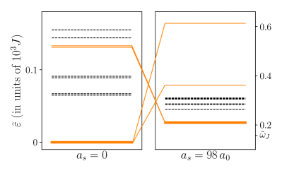
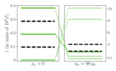
Figure 1: Bare (left) vs. mean-field-shifted (right) single-particle energies of the trapping potentials $V_{A}({\bf r})$ from Ref. [Albiez et al., 2005] (upper panels) and $V_{B}({\bf r})$ from Ref. [LeBlanc et al., 2011] (lower panels). The first ten levels are shown. Thick lines indicate nearly degenerate state pairs. The right panels show the initial renormalization of the levels due to the interaction ($a_{s}=98\,a_{0}$, with $a_{0}$ the Bohr radius). The solid (colored) lines in the right panels are the ones used for the time-dependent numerical calculations (see text). The renormalized Josephson frequency $\tilde{\omega}_{J}$, as extracted from the time evolution of $z(t)$, is also shown for each case.

III Application to experiments

This section is divided into three parts. The first part is dedicated to the quantitative calculation of the trap and interaction parameters for the experiments of Albiez et al.Albiez et al. (2005) and LeBlanc et al.LeBlanc et al. (2011), respectively. In the second part, by scanning through realistic trap-parameter values, we demonstrate numerically that efficient damping can occur only if the resonance condition for the Josephson frequency $\tilde{\omega}_{J}$ and the broadened energy levels of the incoherent excitations $\tilde{\varepsilon}_{m}$ is fulfilled. The third and final part contains our numerical results for experiments with undampedAlbiez et al. (2005) and strongly dampedLeBlanc et al. (2011) Josephson oscillations, respectively.

III.1 Realistic trap parameters and level renormalization

We quantitatively analyze two classes experiments: those of Albiez et al.Albiez et al. (2005) as an exemplary observation of undamped Josephson oscillations, hereafter referred to as experiment (A), and those by LeBlanc et al.LeBlanc et al. (2011) where strong damping occurred, and which we will refer to as experiment (B). Both experiments were performed in double-well potentials, and the population imbalance $z(t)$ between the two wells was traced as a function of time. While the experiments (A) are well described by an effective nonpolynomial Schrödinger equation,Salasnich et al. (2002) in the experiments (B) the Fourier transform of $z(t)$ exhibits two or three frequencies in addition to damping,LeBlanc et al. (2011) indicating contributions from more than two modes.

In order to reduce the numerical effort for the subsequent, time-dependent computations, one should select those levels which participate significantly in the dynamics. To this end, it is important to realize that both,

	$J$	$U$	$J^{\prime}$	$U^{\prime}$	$N$
Albiez et al.Albiez et al. (2005)	$-1.0$	$0.40$	$-0.002$	$0.0001$	$1150$
LeBlanc et al.LeBlanc et al. (2011)	$-1.0$	$1.73$	$-0.006$	$0.0001$	$4500$

Table 1: Hamiltonian matrix elements involving the only left- and right-localized modes, and total particle number $N$ for the experiments (A) of Albiez et al. and (B) of LeBlanc et al., respectively.

the single-particle level energies and the Josephson frequency, are strongly renormalized by the interactions. We calculate the level renormalizations within the BHF approximation at the initial time $t=0$. The bare ($\varepsilon$) and the renormalized ($\tilde{\varepsilon}$) single-particle levels are shown in Fig. 1 for the experiments (A) and (B), respectively, for the example that all particles are initially condensed in the left potential well. It is seen that the interactions even change the sequence of the trap levels. In particular, the two low-lying left- or right-localized levels ($\alpha=1,2$) are shifted upward above the other renormalized levels. The reason is that the two lowest-lying single-particle orbitals are macroscopically occupied by the BEC atoms with condensate population number $N_{\alpha}$, so that the energy for adding one additional particle in these levels is renormalized on the order of $\tilde{\varepsilon}_{\alpha}\approx\varepsilon_{\alpha}+N_{\alpha}U$, with additional contributions from the inter-level condensate interactions $U^{\prime},J^{\prime}$. Similarly, the excited single-particle levels are renormalized predominantly by their interaction with the condensates as $\tilde{\varepsilon}_{n}\approx\varepsilon_{n}+NK_{n}$, $n=3,\,4,\,5,\dots$, where $N=N_{1}+N_{2}$ is the total condensate occupation number and $K_{n}$ substantially smaller than $U$. The interaction-induced re-ordering of levels shown in Fig. 1 remains valid as long as the ground-state occupations $N_{\alpha}$, $\alpha=1,\,2$, are substantial. As a side result, this level re-ordering justifies the frequently used Bogoliubov approximation,Trujillo-Martinez et al. (2009); Posazhennikova et al. (2016, 2018) where non-condensate amplitudes in the left- or right-localized ground modes $\alpha=1,\,2$ are neglected, because such fluctuations are energetically suppressed. Our calculations show that different initial BEC population imbalances $z(0)$ do not significantly alter the renormalized level schemes. In particular, we find that this remains true for the time evolution in both experiments, (A) and (B). Therefore, the initial level renormalization shown in Fig. 1 may be used for selecting the relevant levels at all times during the evolution, see subsection III.3.

	$\varepsilon_{3}$	$\varepsilon_{4}$	$\varepsilon_{5}$	$\varepsilon_{6}$	$U_{3},\,U_{4}$	$U_{5},\,U_{6}$	$K_{3},\,K_{4}$	$K_{5},\,K_{6}$	$R_{\alpha 3},\,R_{\alpha 4}$	$R_{\alpha 5},\,R_{\alpha 6}$	$U^{\prime}_{34}$	$U^{\prime}_{56}$	$U^{\prime}_{35,\,36,\,45,\,46}$
Albiez et al.Albiez et al. (2005)	$131.0$	133.0	–	–	0.075	–	0.055	–	$\pm 0.063$	–	0.075	–	–
LeBlanc et al.LeBlanc et al. (2011)	$189.0$	191.0	381.0	383.0	0.56	0.48	0.33	0.25	$\pm 0.43$	$\pm 0.19$	0.56	0.48	0.29

Table 2: Model parameters involving at least one excited trap mode, $n\geq 3$. Note that $\varepsilon_{4,\,6}=\varepsilon_{3,\,5}+2|J|$.

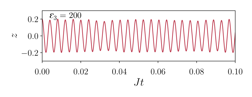
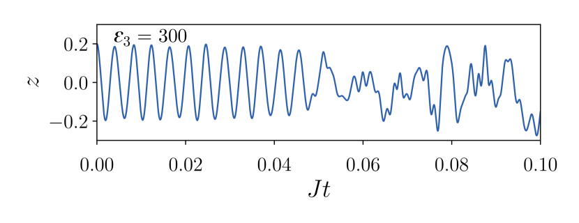
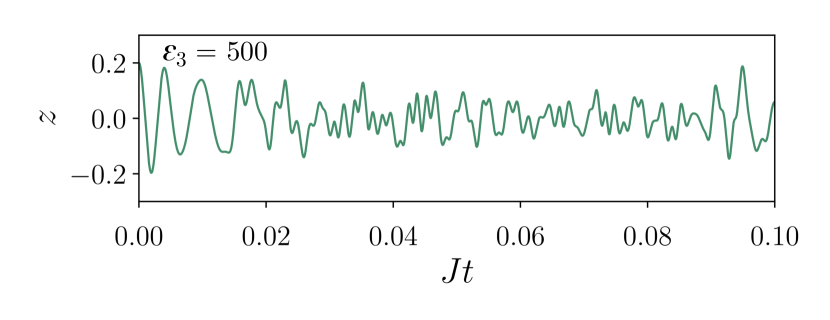
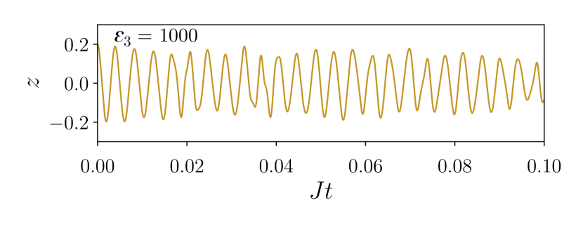
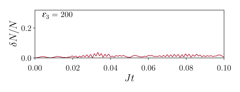
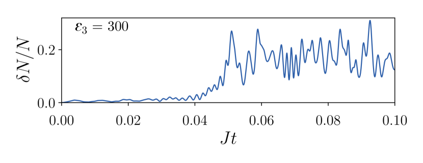
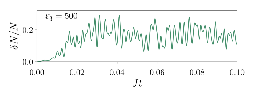
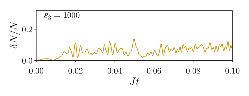
Figure 2: Population imbalance $z(t)$ (left panels) and total fraction of fluctuations $\delta N(t)/N$ (right panels) for $M=3$ modes with $N=5000$ particles, $z(0)=0.2$, initial BEC phase difference $\Delta\theta(0)=0$ and $N_{3}(0)=0$. In all plots, the parameters are $U=1.0$, $U^{\prime}=0$, $J^{\prime}=-0.05$, $U_{3}=0.5$ $K_{3}=0.1$, $R_{\alpha 3}=0.01$, in units of $|J|$. $\varepsilon_{3}$ is varied and has values $\varepsilon_{3}=200,300,500,1000$ (top to bottom), as indicated.

The trap potentials of the two experiments (A) and (B) have different shapes, $V_{A}({\bf r})$ and $V_{B}({\bf r})$, respectively, as given in Appendix B. In order to develop a quantitative description of the dynamics, we solve the (noninteracting) Schrödinger equation with the potentials $V_{A}({\bf r})$ and $V_{B}({\bf r})$ for the first ten single-particle trap wave functions $\varphi_{i}({\bf r})$ and compute the matrix elements of the full Hamiltonian in the trap eigenbasis according to Eqs. (6)-(9). The general interaction matrix elements $U_{ijkl}$ can be classified into intra-level interactions ($U_{\alpha\alpha\alpha\alpha}\equiv U$, $U_{nnnn}\equiv U_{n}$), density-density interactions between different levels ($U_{\alpha\beta\beta\alpha}\equiv U^{\prime}$, $U_{nmmn}\equiv U_{nm}^{\prime}$, $U_{\alpha mm\alpha}\equiv K_{m}$) and interaction-induced transitions between different levels ($U_{\alpha\alpha\alpha\beta}\equiv J^{\prime}$, $U_{\alpha\alpha\alpha m}\equiv R_{\alpha m}$). Here $\alpha,\beta=1,\,2$, $\alpha\neq\beta$, denote the ground modes $\varphi_{1,2}({\bf r})$ localized in the left or right potential well and $n,\,m=3,\,4,\,5,\,\dots$ the higher trap levels. See Appendix B for details of the definitions and calculations. The parameter values computed for a ⁸⁷Rb gas (scattering length $a_{s}\approx 98\,a_{0}$)Vogels et al. (1997) in the experimental setups (A) and (B) are listed in Tabs. 1 and 2. The bare Josephson coupling $J$ turns out to be approximately equal for both experiments, (A) and (B), $J\approx-2\pi\times 0.16\;\mathrm{Hz}$ (see Eq. (II.1) and Appendix B). All energies in this paper are given in units of $|J|$.

III.2 Resonant single-particle excitations

In this subsection, we establish that incoherent excitations (fluctuations) out of the condensate are efficiently created, and therefore that damping occurs, if the frequency of the Josephson oscillations is in resonance with one of the renormalized single-particle levels. The interactions not only renormalize the single-particle levels, but also the Josephson frequency, $\omega_{J}\to\tilde{\omega}_{J}$. Within the two-mode model in the linear regime of Josephson oscillations, it is given bySmerzi et al. (1997)

$$\tilde{\omega}_{J}=2J\sqrt{1+NU/2J}\ .$$ (30)

In the general case of multiple modes and inter-mode interactions it is, however, not possible to give an analytical expression. Therefore, we numerically evolve the interacting system in time for a large number of oscillations, using the Keldysh equation-of-motion method presented in section II, and extract the renormalized Josephson frequency $\tilde{\omega}_{J}$ from the Fourier spectrum of the time-dependent BEC population imbalance $z(t)$. To establish the resonance condition for realistic experimental setups, we consider an exemplary system of three modes with typical parameter values for the experiments (A), (B), given in the caption of Fig. 2, and vary the bare energy $\varepsilon_{3}$ of the third mode above the two lowest modes, whose bare energy we set to $\varepsilon_{1}=\varepsilon_{2}=0$. The corresponding time traces of the BEC population imbalance $z(t)=[N_{1}(t)-N_{2}(t)]/N$ and of the total fraction of noncondensed particles $\delta N(t)/N$ (fluctuations) are shown in Fig. 2. For small and for large level spacings, $\varepsilon_{3}=200,\ 1000$, essentially no fluctuations are generated (right panels), and the Josephson oscillations remain undamped (left panels). However, for intermediate level spacings, $\varepsilon_{3}=300$, and more so for $\varepsilon_{3}=500$, we observe efficient excitation of fluctuations at a characteristic time $\tau_{c}$, and at the same time scale the oscillations become depleted and irregular, but remain reproducible.Trujillo-Martinez et al. (2009) Inelastic interactions between these incoherent excitations (not taken into account at the BHF level of approximation) will lead to rapid damping and eventual thermalization of the Josephson oscillations, as shown in Ref. [Posazhennikova et al., 2016]. To determine the Josephson frequency of the interacting system, $\tilde{\omega}$, we compute the magnitude spectrum of $z(t)$ by fast Fourier transform (FFT) of the time traces up to the time $\tau_{c}$, i.e., before fluctuations are efficiently generated, as shown in Fig. 3. $\tilde{\omega}_{J}$ is given by the position of the pronounced peak in these spectra.

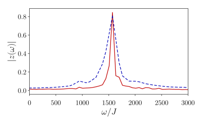
Figure 3: Magnitude spectrum (absolute value of the Fourier transform) of the population imbalance $z(t)$ for the parameters given in Fig. 4 for $\varepsilon_{3}=200$ (solid line) and $\varepsilon_{3}=300$ (dashed line), $N=5000$. The time interval of the FFT was truncated at the onset of the fluctuation regime: for $\varepsilon_{3}=300$, the time trace was cut at $Jt=0.04$, whereas for $\varepsilon_{3}=200$, the entire displayed interval was used.

To analyze now the fluctuation excitation mechanism quantitatively, the renormalized level $\tilde{\varepsilon}_{3}$ as well as the time traces $z(t)$, $\delta N(t)/N$ are computed for a large number of bare $\varepsilon_{3}$ values, and the time-averaged fraction of fluctuations, $\langle\delta N/N\rangle$, is plotted as a function of the ratio $\tilde{\varepsilon}_{3}/\tilde{\omega}_{J}$, see Fig. 4. The figure clearly exhibits resonant behavior: The fluctuation fraction reaches a broad but pronounced maximum when the renormalized level $\tilde{\varepsilon}_{3}$ and the renormalized Josephson frequency $\tilde{\omega}_{J}$ coincide.

We note that this resonant fluctuation-creation mechanism is closely related to, but more general than the dynamical mean-field instabilities reported in Refs. [Castin and Dum, 1997; Vardi and Anglin, 2001; Gerving et al., 2012]. It leads to the highly nonlinear, abrupt creation creation of fluctuationsTrujillo-Martinez et al. (2009) at the characteristic time $\tau_{c}$ seen, e.g., in Fig. 2, panels of the second row ($\varepsilon_{3}=300$). The frequency $\tilde{\omega}_{J}$ acts like the frequency of an external driving field for the subsystem of non-condensate excitations (fluctuations). However, in the present Josephson system the driving is an intrinsic effect, not an external one as in Ref. [Castin and Dum, 1997]. Also, our approach is not restricted to the two-mode scenario,Vardi and Anglin (2001) but can be extended to any number of modes involved. We have tested this for various sets of parameter values and system sizes.

Incoherent excitations will lead to rapid damping and eventual thermalization of the system.Posazhennikova et al. (2016) In order to avoid damping and to stabilize coherent motion, one needs to tune the away from the resonance. One way of achieving this is to change the particle number $N$: While the excitation energies of the not macroscopically occupied levels, $\tilde{\varepsilon}_{n}$, $n\geq 3$, are not strongly affected by $N$, $\tilde{\omega}_{J}$ depends sensitively on $N$ [c.f. Eq.(30)], so that the resonance condition $\tilde{\omega}_{J}\approx\tilde{\varepsilon}_{n}$ (c.f. Fig. 4) may easily be avoided.

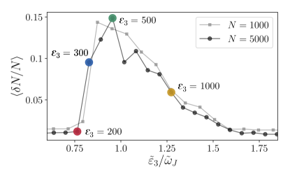
Figure 4: Time-averaged fraction of fluctuations as a function of the ratio of the effective single-particle energy $\tilde{\varepsilon}_{3}$ and the effective Josephson frequency $\tilde{\omega}_{J}$ for two different particle numbers (the small, gray squares are for $N=1000$, the small, black circles are for $N=5000$, corresponding to experiments (A) and (B), respectively). The interaction parameters are $U=1.0$, $U^{\prime}=0$, $J^{\prime}=-0.05$, $U_{3}=0.5$, $K_{3}=0.1$, $R_{\alpha 3}=0.01$, and the initial conditions: initial population imbalance $z(0)=0.2$, initial phase difference $\Delta\theta(0)=0$, $M=3$, and $N_{3}(0)=0$. The renormalized Josephson frequency is extracted from the Fourier transforms of $z(t)$: $\tilde{\omega}_{J}\approx 1571$ for $N=5000$, and $\tilde{\omega}_{J}\approx 315$ for $N=1000$. The time average of the fluctuations was taken over the displayed time interval for $N=5000$, whereas for $N=1000$ an interval of 5 times that size was used. The thick dots represent the results for the time traces of Fig. 2 for the corresponding values of $\varepsilon_{3}$, as indicated in the figures.

III.3 Comparison with experiments

We now examine how the experiments (A) and (B) fit into the resonant-fluctuation-creation scenario described above.

	$N$	$z(0)$	$N_{1}$	$N_{2}$	$N_{3}$	$N_{4}$	$N_{5}$	$N_{6}$
Albiez et al.Albiez et al. (2005)	1150	0.290	742	408	0	0	–	–
LeBlanc et al.LeBlanc et al. (2011)	4500	0.116	2436	1914	75	75	0	0

Table 3: Occupation numbers at time $t=0$ used for the numerical calculations.

In Fig. 5 we give the results of our calculations for the experimental setup (A) of Albiez et al. Albiez et al. (2005) with the four relevant modes shown in Fig. 1 in direct comparison with the experimental data points. Note that there is no fitting of parameters involved. We see that the agreement with the experiment is very good regarding both the frequency and the amplitude of the Josephson oscillations. In particular, no damping is observed in the experiment as well as in the calculation. The fraction of fluctuations remains below 10 $\%$, indicating that this experimental setup is away from the resonance discussed in Fig. 4.

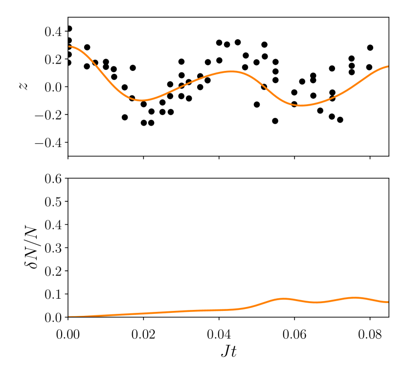
Figure 5: Population imbalance $z(t)$ and relative fraction of fluctuations $\delta N(t)/N$ for the experiments (A). Albiez et al. (2005) The experimental data points (black dots) are taken from the reference. The parameters and initial conditions for the calculations are listed in Tabs. 1 – 3.

In Fig. 6 we display the corresponding calculations for the experiment (B).LeBlanc et al. (2011) We took six relevant modes into account in our calculations, as explained in the discussion of Fig. 1. For this experiment we assume a small initial condensate occupation of the modes $m=3,\,4$, as listed in Tab. 3, because of the small excitation energy of these modes (see Fig. 1) with regard to the larger interaction parameters of experiment (B). Here the agreement with experiment is quantitatively not as good as for the experiment (A).Albiez et al. (2005) However, the theoretical calculation reproduces the strong amplitude reduction of $z(t)$ after a short time of only $t\approx 0.004\leavevmode\nobreak\ J$ in agreement with experiment. At the same time, the calculation shows a fast and efficient excitation of fluctuations, which set in at a characteristic time scalePosazhennikova et al. (2016) of $\tau_{c}\approx 0.0013\leavevmode\nobreak\ J$ and reach a maximum amplitude of about $\delta N_{max}/N\approx 0.5$ near the time $t\approx 0.0035\leavevmode\nobreak\ J$. This indicates that this experimental setup is in the resonant regime. Importantly, we find that the efficient creation of fluctuations for the parameters of experiment (B) is robust, independent of the small condensate occupation of the modes with $m=3,\,4$ as well as the precise value of $N$.

The reason for the reduced quantitative agreement with experiment can be understood from the behavior of the fluctuation fraction. As seen in Fig. 6, lower panel, the departure of the theoretical results from the experimental data points is significant for those times when the non-condensate fraction $\delta N(t)/N$ is large. A large fraction of fluctuations means that the BHF approximation employed in the present work is not sufficient, and higher-order corrections should be taken into account. They account for inelastic collisions of excitations and will, therefore, lead to rapid damping,Posazhennikova et al. (2016) as observed in experiment (B).LeBlanc et al. (2011)

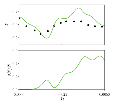
Figure 6: Population imbalance $z(t)$ and relative fraction of fluctuations $\delta N(t)/N$ for the experiments (B). LeBlanc et al. (2011) The experimental data points (black dots) are taken from the reference. The parameters and initial conditions for the calculations are listed in Tabs. 1 – 3.

IV Discussion and conclusion

We have considered Josephson oscillations of isolated, atomic BECs trapped in double-well potentials and analyzed the impact of fluctuations, i.e. out-of-condensate particle excitations, on the dynamics of the oscillations for the two specific experiments of Albiez et al. (A),Albiez et al. (2005) and of LeBlanc et al. (B).LeBlanc et al. (2011) While the first experiment is well described by Gross-Pitaevskii dynamics,Smerzi et al. (1997) suggesting a negligible role played by the fluctuations, the latter experiment exhibits fast relaxation of the oscillations, which is not contained in the semiclassical Gross-Pitaevskii description, even if multiple trap modes are considered. One therefore expects a sizable number of non-condensate excitations created in this experiment.

We identified a scenario for the resonant excitation of fluctuations. It indicates that, whenever any of the renormalized trap levels is close to the effective Josephson frequency, this leads to resonant creation of fluctuations and a departure from the Gross-Pitaevskii dynamics. The interaction-induced renormalization of both the trap levels as well as the Josephson frequency is important for this resonant effect to occur. By numerical calculations for the realistic model parameters, we showed that indeed experiment (A) is off resonance with only a small amount of fluctuations created, while experiment (B) is operated in the resonant regime and dominated by fluctuations. This reconciles the qualitatively different behavior of the two experiments. In another, more recent experimentSpagnolli et al. (2017) the bare Josephson frequency $\omega_{J}$ was chosen smaller than the trap level spacings (see Supplemental Information to Ref. [Spagnolli et al., 2017]), and the BJJ oscillation frequency was further reduced by tuning the interaction $U$ to become attractive. Thus, this experiment is in the off-resonant regime. Indeed, it shows extended undamped oscillations. It is well described by GPE dynamics aloneSpagnolli et al. (2017), as expected.

As a more general conclusion, for the design of long-lived, coherent Josephson junctions it is essential to ensure that none of the renormalized and possibly interaction-broadened trap levels is on resonance with the effective Josephson frequency. This can be achieved by either tuning the parameters of the trap or by adjusting the total number of particles. In this way, Bose-Josephson junctions may serve as a device for studying the departure from classicality due to quantum fluctuations in a controlled way.

APPENDIX A: TWO-MODE APPROXIMATION

To illustrate the details of the formalism, we present here the derivation of the equations of motion for a two-mode system where, however, the out-of-condensate fluctuations are taken into account in each mode. In this respect, the calculation goes beyond the two-mode model studied at the semiclassical (Gross-Pitaevskii) level of approximation in Refs. [Smerzi et al., 1997; Ananikian and Bergeman, 2006]. For clarity of presentation, we here discard the nonlocal (inter-mode) interaction parameters. The important steps to be demonstrated in this appendix carry over to the general case used to describe the experiments (multi-mode, nonlocal interactions) in a straightforward manner. For the scope of this appendix, the action hence reads,

$$S=S_{0}+\sum_{\alpha=1}^{2}S_{\text{int}}[\phi_{\alpha}^{*},\phi_{\alpha}],$$

where

$$S_{0}=\int\text{d}t\left[\sum_{\alpha=1}^{2}\left(\phi_{\alpha}^{*}G_{0}^{-1}\phi_{\alpha}\right)-J\left(\phi_{1}^{*}\phi_{2}+\phi_{2}^{*}\phi_{1}\right)\right],$$ (31)

and

$$S_{\text{int}}[\phi^{*},\phi]=-\tfrac{U}{2}\int\text{d}t\,\left|\phi\right|^{4}.$$ (32)

Writing the corresponding Keldysh action explicitly, one finds

$$\begin{split}&S_{K}[\Phi_{c},\Phi_{q}]=\int\text{d}t\bigg{\{}\sum_{\alpha=1}^{2}\left[\right.\phi^{*}_{\alpha\,q}\left(\mathrm{i}\,\partial_{t}-\varepsilon\right)\phi_{\alpha\,c}\\ &+\phi^{*}_{\alpha\,c}\left(\mathrm{i}\,\partial_{t}-\varepsilon\right)\phi_{\alpha\,q}\left.\right]-J\left[\phi_{1\,q}^{*}\phi_{2\,c}+\phi_{1\,c}^{*}\phi_{2\,q}+\text{c.c.}\right]\\ &-\tfrac{U}{2}\sum_{\alpha=1}^{2}\left[\phi_{\alpha\,c}^{*}\phi_{\alpha\,c}^{*}\phi_{\alpha\,c}\phi_{\alpha\,q}+\phi^{*}_{\alpha\,q}\phi^{*}_{\alpha\,q}\phi_{\alpha\,q}\phi_{\alpha\,c}+\text{c.c.}\right]\bigg{\}}.\end{split}$$ (33)

Performing the variation according to Eq. (18) yields the modified Gross-Pitaevskii equation (GPE) as the saddle-point equation of our action:

$$\begin{split}\mathrm{i}\partial_{t}\Phi_{1\,c}&=\varepsilon\Phi_{1\,c}+J\Phi_{2\,c}+\tfrac{U}{2}\Phi^{*}_{1\,c}\Phi_{1\,c}\Phi_{1\,c}\\ &+\tfrac{U}{2}(\Phi_{1\,q}\Phi_{1\,q}\Phi^{*}_{1\,c}+2\Phi^{*}_{1\,q}\Phi_{1\,q}\Phi_{1\,c}\\ &+2\langle\delta\phi_{1\,c}\delta\phi^{*}_{1\,c}\rangle\Phi_{1\,c}+\langle\delta\phi_{1\,c}\delta\phi_{1\,c}\rangle\Phi^{*}_{1\,c}\\ &+2\langle\delta\phi_{1\,c}\delta\phi_{1\,q}\rangle\Phi^{*}_{1\,q}+2(\langle\delta\phi_{1\,c}\delta\phi^{*}_{1\,q}\rangle+\text{c.c.})\Phi_{1\,q}\\ &+2\langle\delta\phi_{1\,q}\delta\phi^{*}_{1\,q}\rangle\Phi_{1\,c}+\langle\delta\phi_{1\,q}\delta\phi_{1\,q}\rangle\Phi^{*}_{1\,c}).\end{split}$$ (34)

Taking into account that $\Phi_{1\,q}=\Phi^{*}_{1\,q}=0$, as well as the fact that all Green functions of two quantum fields vanish because of the relation between (anti-) time-ordered, greater and lesser Green functions, by letting $\Phi_{\alpha\,c}=\Phi_{\alpha}$ we obtain the final form of our modified GPE as

$$\mathrm{i}\partial_{t}\Phi_{1} =\varepsilon\Phi_{1}+J\Phi_{2}+\tfrac{U}{2}\Phi^{*}_{1}\Phi_{1}\Phi_{1},$$

$$+\tfrac{U}{2}(\langle\delta\phi_{1\,c}\delta\phi_{1\,c}\rangle\Phi^{*}_{1}+2\langle\delta\phi_{1\,c}\delta\phi^{*}_{1\,c}\rangle\Phi_{1}),$$ (35)

which upon introduction of the fluctuation Green functions reads

$$\mathrm{i}\partial_{t}\Phi_{1}= (\varepsilon+\tfrac{U}{2}\Phi^{*}_{1}\Phi_{1})\Phi_{1}+J\Phi_{2}+\mathrm{i}U(\,G_{11}\,\Phi_{1}+\tfrac{1}{2}\,g_{11}\,\Phi^{*}_{1}).$$ (36)

The equation for the second field can be obtained by substituting $2\leftarrow 1$ and vice versa. Next we calculate the second derivatives of the effective action and find

$$\frac{\delta^{2}\Gamma}{\delta\Phi_{\alpha\,q}^{*}(t)\delta\Phi_{\alpha\,c}(t)} =\mathrm{i}\partial_{t}-\varepsilon-U\left(\Phi^{*}_{\alpha}\Phi_{\alpha}+\mathrm{i}G_{\alpha\alpha}\right),$$ (37)

$$\frac{\delta^{2}\Gamma}{\delta\Phi_{\alpha\,q}^{*}(t)\delta\Phi_{\alpha\,c}^{*}(t)} =-\tfrac{U}{2}\left(\Phi^{\,2}_{\alpha}+\mathrm{i}g_{\alpha\alpha}\right),$$ (38)

whereas the off-diagonals in level space are simply

$$\frac{\delta^{2}\Gamma}{\delta\Phi_{1\,q}^{*}(t)\delta\Phi_{2\,c}(t)} =-J,$$ (39)

$$\frac{\delta^{2}\Gamma}{\delta\Phi_{1\,q}^{*}(t)\delta\Phi_{2\,c}^{*}(t)} =0.$$ (40)

Now make the ansatz

$$\Phi_{\alpha}=\sqrt{2N_{\alpha}}\,e^{\mathrm{i}\varphi_{\alpha}}$$ (41)

for the condensate fields. Subtracting Eq. (22) and the corresponding advanced equation, and taking the upper left component of the matrices in Bogoliubov space, one finds, after performing the equal-time limit on the Green functions $G_{\alpha\beta}(t,t^{\prime})$, that

$$\begin{split}\mathrm{i}\partial_{t}G_{11}+N_{1}U(e^{-2\mathrm{i}\varphi_{1}}{g_{11}}+\text{c.c.})+J(G_{12}-G_{21})&=0,\\ \mathrm{i}\partial_{t}G_{22}+N_{2}U(e^{-2\mathrm{i}\varphi_{2}}{g_{22}}+\text{c.c.})-J(G_{12}-G_{21})&=0,\end{split}$$ (42)

where $G_{\alpha\beta}=G_{\alpha\beta}(t)=G_{\alpha\beta}(T=t,\tau=0)$ depends only on the average time $T=(t+t^{\prime})/2=t$ after taking $t^{\prime}\to t$.

The same holds for the anomalous Green functions. Accordingly, adding Eq. (22) and the corresponding advanced equation, and taking the upper right component in Bogoliubov space, one finds for the anomalous Green functions, e.g.

$$\mathrm{i}\partial_{t}g_{\alpha\alpha} -2(\varepsilon+2N_{\alpha}U+\mathrm{i}UG_{\alpha\alpha})g_{\alpha\alpha}$$

$$-U\left(2N_{\alpha}e^{2\mathrm{i}\varphi_{\alpha}}+\mathrm{i}g_{\alpha\alpha}\right)G_{\alpha\alpha}-2Jg_{12}=0.$$ (43)

The remaining equations are

$$\begin{split}&\mathrm{i}\partial_{t}G_{12}-U\left(2(N_{1}-N_{2})+\mathrm{i}G_{11}-\mathrm{i}G_{22}\right)G_{12}+J(G_{11}-G_{22})\\ &+\tfrac{U}{2}\left[\right.g_{12}^{*}(\Phi_{1}\Phi_{1}+\mathrm{i}g_{11})+g_{12}(\Phi_{2}^{*}\Phi_{2}^{*}-\mathrm{i}g_{22}^{*})\left.\right]=0,\end{split}$$ (44)

and

$$\begin{split}&\mathrm{i}\partial_{t}g_{12}-2\varepsilon g_{12}+U\sum_{\alpha}(2N_{\alpha}+\mathrm{i}G_{\alpha\alpha})g_{12}-J\sum_{\alpha}g_{\alpha\alpha}\\ &+\tfrac{U}{2}\left[G_{12}^{*}(\Phi_{1}\Phi_{1}+\mathrm{i}g_{11})-G_{12}(\Phi_{2}^{*}\Phi_{2}^{*}+\mathrm{i}g_{22})\right]=0,\end{split}$$ (45)

together with the identities $G_{21}(t)=-G_{12}^{*}(t)$ and $g_{21}(t)=g_{12}(t)$.

With $G_{\alpha\alpha}=-\mathrm{i}F_{\alpha}$, where

$$F_{\alpha}=2\delta N_{\alpha}+1,$$ (46)

one obtains for the total number of fluctuations

$$\delta\dot{N}=\delta\dot{N}_{1}+\delta\dot{N}_{2}=-\sum_{\alpha=1}^{2}\tfrac{N_{\alpha}U}{2}(e^{-2\mathrm{i}\varphi_{\alpha}}{g_{\alpha\alpha}}+\text{c.c.}).$$ (47)

Defining the phase difference of the two condensates as $\Delta\varphi=\varphi_{2}-\varphi_{1}$, from Eq. (36) one calculates

$$\dot{N}_{1} =+2J\sqrt{N_{1}N_{2}}\sin{\Delta\varphi}+\tfrac{N_{1}U}{2}(e^{-2\mathrm{i}\varphi_{1}}{g_{11}}+\text{c.c.}),$$

$$\dot{N}_{2} =-2J\sqrt{N_{1}N_{2}}\sin{\Delta\varphi}+\tfrac{N_{2}U}{2}(e^{-2\mathrm{i}\varphi_{2}}{g_{22}}+\text{c.c.}),$$ (48)

which resonates with the results from Ref. [Smerzi et al., 1997], with the additional contributions from the fluctuations. It should be noted here that $J<0$ in our convention.

One clearly sees from (47) and (APPENDIX A: TWO-MODE APPROXIMATION) that the total particle number $N$ is conserved,

$$\partial_{t}\sum_{\alpha}\left(N_{\alpha}+\delta N_{\alpha}\right)=\dot{N}=0\ .$$ (49)

Similarly, by employing the dynamical equations (42), (APPENDIX A: TWO-MODE APPROXIMATION) and (44), the total energy

$$E=\tfrac{1}{2}\sum_{\alpha}\,\left(E_{\alpha}^{c}+E_{\alpha}^{q}\right),$$ (50)

with the condensate energy

$$\begin{split}E_{\alpha}^{c}=2UN_{\alpha}^{2}+2UF_{\alpha}N_{\alpha}&+\tfrac{U}{4}\left(\mathrm{i}g_{\alpha\alpha}\Phi_{\alpha}^{*}\Phi_{\alpha}^{*}+\text{c.c.}\right)\\ &+J\left(\Phi_{1}^{*}\Phi_{2}+\text{c.c.}\right),\end{split}$$ (51)

and the fluctuation energy

$$\begin{split}E_{\alpha}^{q}&=UF_{\alpha}\left(2N_{\alpha}+F_{\alpha}\right)+\tfrac{U}{2}g_{11}^{*}g_{11}\\ &+\tfrac{U}{4}\left(\mathrm{i}g_{\alpha\alpha}\Phi_{\alpha}^{*}\Phi_{\alpha}^{*}+\text{c.c.}\right)+\mathrm{i}J\left(G_{12}-G_{12}^{*}\right),\end{split}$$ (52)

may be shown to be conserved,

$$\mathrm{i}\partial_{t}E=0.$$ (53)

APPENDIX B: COMPUTATION OF TRAP PARAMETERS

IV.1 Diagonalization of trap potentials

The trap potential employed in experiment Ref. [Albiez et al., 2005] reads

$$V_{A}({\bf r})=\tfrac{m}{2}\left[\omega_{x}^{2}x^{2}+\omega_{y}^{2}y^{2}+\omega_{z}^{2}z^{2}\right]+\tfrac{V_{0}}{2}\left[1+\cos{\left(\tfrac{2\pi x}{d}\right)}\right],$$ (54)

with frequencies given in Ref. [Albiez et al., 2005]. Since a Hamiltonian with this potential is separable, the eigenfunctions are the products of the eigenfunctions in each spatial dimension. Hence, the diagonalization of the noninteracting trap system reduces to three separate diagonalizations, which can be performed by applying standard library methods (e.g. Ref. [Guennebaud et al., 2010]), yielding all eigenvalues and eigenfunctions of the trap.

The confining potential of the experiment Ref. [LeBlanc et al., 2011] is more involved,

$$V_{B}({\bf r}) =m^{\prime}_{F}\hbar\sqrt{\delta(\mathbf{r})^{2}+\left(\frac{\mu_{\text{B}}g_{F}B_{\text{RF},\perp}(\mathbf{r})}{2\hbar}\right)^{2}}+\tfrac{m}{2}\omega_{y}^{2}y^{2},$$ (55)

where $\delta(\mathbf{r})=\omega_{\text{RF}}-\left|\mu_{\text{B}}g_{F}B_{S}(\mathbf{r})/\hbar\right|$, see Ref. [LeBlanc et al., 2011]) for details and the definition of the parameters. We use the parameter values quoted there with $\delta=2\pi\times(-0.4)$. Since Eq. (55) is not separable along the spatial axes, the Hamiltonian dimension is too large for direct numerical diagonalization. In order to be as close to the actual experiment as possible, we expressly do not approximate Eq. (55) by an expression that would be easily accessible numerically. Therefore, one has to resort to an algorithm that can handle very large matrices. We employ the Jacobi-Davidson algorithm.Geus (2002); Davidson (1975) It is an iterative subspace method that iteratively returns the first few eigenvalues and eigenvectors of a high-dimensional problem. Note that for the present analysis it is essential to include higher trap states. As examples of the results, the wave functions of three different trap eigenstates for the nonseparable potential, Eq. (55), are shown in Fig. 7.

IV.2 Computation of the interaction parameters

For the experiments (A) and (B), many of the parameters of Eq. (9) turn out to be negligible, such that, retaining only the significant parameters, the interacting part of the action can be simplified to $S_{\text{int}}=-\tfrac{1}{2}\left(S_{\text{loc}}+S_{12}+S_{mn}+S_{\alpha m}\right),$ with

$$\begin{split}S_{\text{loc}}=&\int\text{d}t\left(U\sum_{\alpha=1}^{2}\,\left|\phi_{\alpha}\right|^{4}+\sum_{m=3}^{M}U_{m}\left|\phi_{m}\right|^{4}\right),\end{split}$$ (56)

$$\begin{split}S_{12}=&\int\text{d}t\;\left[\right.U^{\prime}\left({\phi_{1}^{*}\phi_{1}^{*}}{\phi_{2}\phi_{2}}+2\,{\phi_{1}^{*}\phi_{1}}{\phi_{2}^{*}\phi_{2}}\right)\\ &+2J^{\prime}\left({\phi_{1}^{*}\phi_{1}^{*}\phi_{1}}{\phi_{2}}+{\phi_{2}^{*}\phi_{2}^{*}\phi_{2}}{\phi_{1}}\right)+\text{c.c.}\left.\right],\end{split}$$ (57)

$$S_{mn}=\int\text{d}t\;\sum_{\begin{subarray}{c}m,\,n=3\\ m\neq n\end{subarray}}^{M} \tfrac{1}{2}U^{\prime}_{mn}({\phi_{m}^{*}\phi_{m}^{*}}{\phi_{n}\phi_{n}}+2\,{\phi_{m}^{*}\phi_{m}}{\phi_{n}^{*}\phi_{n}}+\text{c.c.}),$$ (58)

$$S_{\alpha m}= \int\text{d}t\;\sum_{\alpha=1}^{2}\sum_{m=3}^{M}\left[\right.K_{m}\left({\phi_{\alpha}^{*}\phi_{\alpha}^{*}}{\phi_{m}\phi_{m}}+2\,{\phi_{\alpha}^{*}\phi_{\alpha}}{\phi_{m}^{*}\phi_{m}}\right)$$

$$+2R_{\alpha m}{\phi_{\alpha}^{*}\phi_{\alpha}^{*}\phi_{\alpha}}{\phi_{m}}+\text{c.c.}\left.\right].$$ (59)

The parameters introduced in Eqs. (56) – (IV.2) are defined by

$$U =\tilde{g}\int\text{d}^{3}r\,\varphi_{\alpha}^{4}(\mathbf{r}),\quad\alpha=1,\,2$$ (60)

$$U_{m} =\tilde{g}\int\text{d}^{3}r\,\varphi_{m}^{4}(\mathbf{r}),\quad m\geq 3$$ (61)

$$U^{\prime} =\tilde{g}\int\text{d}^{3}r\,\varphi_{1}^{2}(\mathbf{r})\varphi_{2}^{2}(\mathbf{r})$$ (62)

$$J^{\prime} =\tilde{g}\int\text{d}^{3}r\,\varphi_{1}^{3}(\mathbf{r})\varphi_{2}(\mathbf{r})$$ (63)

$$U^{\prime}_{mn} =\tilde{g}\int\text{d}^{3}r\,\varphi_{m}^{2}(\mathbf{r})\varphi_{n}^{2}(\mathbf{r}),\quad m,\,n\geq 3$$ (64)

$$K_{m} =\tilde{g}\int\text{d}^{3}r\,\varphi_{\alpha}^{2}(\mathbf{r})\varphi_{m}^{2}(\mathbf{r}),\quad\alpha=1,\,2;\ m\geq 3$$ (65)

$$R_{\alpha m} =\tilde{g}\int\text{d}^{3}r\,\varphi_{\alpha}^{3}(\mathbf{r})\varphi_{m}(\mathbf{r}),\quad\alpha=1,\,2;\ m\geq 3$$ (66)

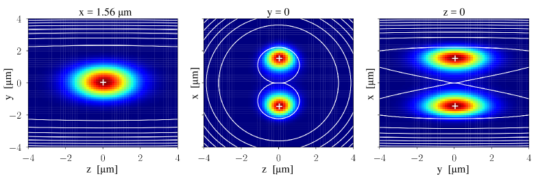
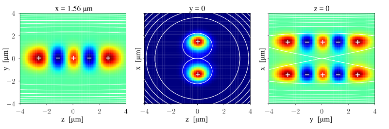
Figure 7: Spatial profiles of eigenfunctions of the trap potential Eq. (55), where the double-well is orianted along the $z$ axis. Top row: the symmetric state $\varphi_{+}(\mathbf{r})$; middle row: the antisymmetric state $\varphi_{-}(\mathbf{r})$; bottom row: the symmetric state corresponding to the uppermost thick level in Fig. 1 for $a_{s}=0$. The cuts shown are along the $y-z$ plane for $x=x_{min}=1.56\leavevmode\nobreak\ \mu$m (position of the trap minimum), along the $z-x$ plane for $y=0$, and along the $x-y$ plane for $z=0$, respectively, as indicated. The color or gray scale describes the wave function amplitude (arbitrary units). $+$ ($-$) signs indicate the regions of positive (negative) extrema of the wave function. In the panels without sign change, the zero level of the wave function is represented by dark blue (dark gray), while in the panels with sign change, the zero level is represented by light green (light gray). Some of the trap equipotential lines are shown as white lines, providing a guide to the eye where the minima of the trap potential are located. This solution was obtained with the Jacobi-Davidson algorithm for a spatial resolution of $64$ grid points in each spatial dimension.

References

- Smerzi et al. (1997) A. Smerzi, S. Fantoni, S. Giovanazzi, and S. R. Shenoy, Phys. Rev. Lett. 79, 4950 (1997).
- Albiez et al. (2005) M. Albiez, R. Gati, J. Fölling, S. Hunsmann, M. Cristiani, and M. K. Oberthaler, Phys. Rev. Lett. 95, 010402 (2005).
- Levy et al. (2007) S. Levy, E. Lahoud, I. Shomroni, and J. Steinhauer, Nature 449, 579 (2007).
- LeBlanc et al. (2011) L. J. LeBlanc, A. B. Bardon, J. McKeever, M. H. T. Extavour, D. Jervis, J. H. Thywissen, F. Piazza, and A. Smerzi, Phys. Rev. Lett. 106, 025302 (2011).
- Spagnolli et al. (2017) G. Spagnolli, G. Semeghini, L. Masi, G. Ferioli, A. Trenkwalder, S. Coop, M. Landini, L. Pezzè, G. Modugno, M. Inguscio, A. Smerzi, and M. Fattori, Phys. Rev. Lett. 118, 230403 (2017).
- Posazhennikova et al. (2018) A. Posazhennikova, M. Trujillo-Martinez, and J. Kroha, Ann. Phys. (Berlin) 530, 1700124 (2018).
- Posazhennikova et al. (2016) A. Posazhennikova, M. Trujillo-Martinez, and J. Kroha, Phys. Rev. Lett. 116, 225304 (2016).
- (8) M. Lenk, T. Lappe, A. Posazhennikova, and J. Kroha, to be published .
- Deutsch (1991) J. M. Deutsch, Phys. Rev. A 43, 2046 (1991).
- Srednicki (1994) M. Srednicki, Phys. Rev. E 50, 888 (1994).
- Ananikian and Bergeman (2006) D. Ananikian and T. Bergeman, Phys. Rev. A 73, 013604 (2006).
- Vogels et al. (1997) J. M. Vogels, C. C. Tsai, R. S. Freeland, S. J. J. M. F. Kokkelmans, B. J. Verhaar, and D. J. Heinzen, Phys. Rev. A 56, R1067 (1997).
- van Kempen et al. (2002) E. G. M. van Kempen, S. J. J. M. F. Kokkelmans, D. J. Heinzen, and B. J. Verhaar, Phys. Rev. Lett. 88, 093201 (2002).
- Keldysh (1964) L. V. Keldysh, JETP 20, 1080 (1964).
- Sieberer et al. (2016) L. M. Sieberer, M. Buchhold, and S. Diehl, Rep. Prog. Phys. 79, 096001 (2016).
- Jackiw (1974) R. Jackiw, Phys. Rev. D 9, 1686 (1974).
- Trujillo-Martinez et al. (2015) M. Trujillo-Martinez, A. Posazhennikova, and J. Kroha, New J. Phys. 17, 013006 (2015).
- Salasnich et al. (2002) L. Salasnich, A. Parola, and L. Reatto, Phys. Rev. A 65, 043614 (2002).
- Trujillo-Martinez et al. (2009) M. Trujillo-Martinez, A. Posazhennikova, and J. Kroha, Phys. Rev. Lett. 103, 105302 (2009).
- Castin and Dum (1997) Y. Castin and R. Dum, Phys. Rev. Lett. 79, 3553 (1997).
- Vardi and Anglin (2001) A. Vardi and J. R. Anglin, Phys. Rev. Lett. 86, 568 (2001).
- Gerving et al. (2012) C. S. Gerving, T. M. Hoang, B. J. Land, M. Anquez, C. D. Hamley, and M. S. Chapman, Nature Commun. 3, 1169 (2012).
- Guennebaud et al. (2010) G. Guennebaud, B. Jacob, and Others, “Eigen v3,” http://eigen.tuxfamily.org (2010).
- Geus (2002) R. Geus, Dissertation (2002), 10.3929/ethz-a-004469464.
- Davidson (1975) E. R. Davidson, J. Comput. Phys. 17, 87 (1975).