Direct optimisation of the discovery significance when training neural networks to search for new physics in particle colliders

Abstract

We introduce two new loss functions designed to directly optimise the statistical significance of the expected number of signal events when training neural networks to classify events as signal or background in the scenario of a search for new physics at a particle collider. The loss functions are designed to directly maximise commonly used estimates of the statistical significance, $s/\sqrt{s+b}$, and the Asimov estimate, $Z_{A}$. We consider their use in a toy SUSY search with 30 fb^-1 of 14 TeV data collected at the LHC. In the case that the search for the SUSY model is dominated by systematic uncertainties, it is found that the loss function based on $Z_{A}$ can outperform the binary cross entropy in defining an optimal search region.

1 Introduction

Data analysis in High Energy Physics (HEP) is a genuine multivariate classification problem. In particle colliders, the results of collisions that are recorded by detectors, such as ATLAS and CMS at the LHC, are reconstructed to determine the subatomic particles produced in each collision. In searches for new physics, a multivariate analysis is carried out with these quantities to distinguish between the Standard Model (SM) background processes and potential signal from physical processes that are not predicted within the SM.

Traditional searches for new physics, such as supersymmetry [1, 2, 3, 4, 5, 6, 7, 8], approach this by designing discriminative high level variables, based on the result of the event reconstruction. These variables usually exploit differences in energy scale or topology between the signal and background processes. The design of these variables requires significant prior physics knowledge. Additionally, this approach may not take into account all of the subtle differences between signal and background events.

There have been significant advances in the power and viability of using neural networks for such discrimination problems in recent years, mainly driven by the accessibility of large datasets and advances in computing power. Deep neural networks have the promise to approach the background and signal classification problem from low level reconstructed quantities. They are then able to find sophisticated ways to discriminate between signal and background, finding details above and beyond those contained in the high level variables [9].

When a new physics search is framed as a signal and background classification problem, the search is actually designed to maximise the statistical significance of the signal sample over the background sample, rather than obtaining the best classification accuracy or receiver operating characteristic (ROC). This translates to a maximisation of the correct classification of signal events, while minimising the incorrect classification of background events. In this case, the classification of signal events as background events is tolerable, providing the overall purity of the signal classification is maintained. Many of the approaches for optimisation of classification problems with neural networks, such as the minimisation of the cross entropy, give the same weight to the correct classification of signal events as to the correct classification of background events. In this paper, we consider an alternative optimisation approach that directly maximises the statistical significance of the selected signal. This gives more priority to the purity of the signal classification than the purity of the background classification.

2 An example search for a third-generation supersymmetric quark partner

As a physics example we consider a toy search for supersymmetric top quarks at the LHC. The search is designed for the case of direct top squark pair production with subsequent decay of each squark into a top quark and the lightest supersymmetric particle (LSP). We assume that the top squark and the LSP are the only SUSY particles that have low enough masses to be accessible at the LHC. In a real search, limits are typically set as a function of the top squark and the neutralino masses. In the context of SUSY searches models are often categorised in two different ways. In the cases that the top squark is much heavier than the LSP, the SM decay products are produced with significant energy, making them easy to observe in the detector. These models are known as uncompressed. In the case that the difference in mass between the top squark and LSP is small, the SM decay products are produced close to rest, making the signature much more difficult to distinguish from the background. These models are known as compressed.

For our toy study, we assume two sets of mass parameters that are expected to be on the border of discovery with about 30$\,\text{fb}^{\text{$-$1}}$ of 14 TeV data collected at the LHC. We consider an uncompressed point with the top squark mass fixed at 900 GeV and the neutralino mass at 100 GeV. We additionally consider a compressed mass point with a top squark mass of 600 GeV and a neutralino mass of 400 GeV, where the mass splitting is at the order of the top mass. These two points present different challenges, the uncompressed point has a low cross section, meaning few signal events are expected to be produced. The compressed point has a higher cross section but is harder to distinguish from the background. As background, we consider only the dominant process of top-antitop ($\it{t}\overline{\it{t}}$) production. This background is several orders of magnitude higher than the signal, and the distributions of signal and background variables are quite similar, due to their comparable kinematics.

A leading-order simulation is sufficient for our purpose and we only take into account next-to-leading order results for the total cross sections of stop signal [10] and $\it{t}\overline{\it{t}}$ background [11, 12]. Cross sections of 17.6 fb for the uncompressed model, 228 fb for the compressed model and 844 fb for the $\it{t}\overline{\it{t}}$ background are used. Pythia8 [13, 14] is used for the event simulation and Delphes3 [15] to model the detector response using the Delphes model of the CMS detector. Jets are clustered with anti-$k_{T}$ [16] with a cone parameter of $R=0.4$ and we use lepton as a generic term for electrons and muons. For simplicity, we do not consider tau leptons since their experimental reconstruction is more complex.

In order to reduce the training times, while retaining most of the events of interest, signal and background events are pre-selected. We require at least one lepton with transverse momentum $p_{\mathrm{T}}>30\,\text{GeV}$ within a pseudorapidity of $|\eta|<2.4$. Each event must contain at least four jets with $p_{\mathrm{T}}>40\,\text{GeV}$, where the highest-$p_{\mathrm{T}}$ (leading) jet is required to have $p_{\mathrm{T}}>80\,\text{GeV}$, and the sub-leading jet $p_{\mathrm{T}}>60\,\text{GeV}$. At least one of the jets must be tagged as originating from a bottom quark. The missing energy perpendicular to the beam direction (the negative vector sum of the momenta of all reconstructed particles), $E_{\mathrm{T}}/\kern 4.49997pt$, is required to be above 200 GeV, and the scalar sum over the transverse momenta of all preselected jets, $H_{\mathrm{T}}$, to be above 300 GeV. After this preselection, the remaining background is still several orders of magnitude higher than the investigated signal. This setup is similar to the one used in [17] where more details can be found. The selected sample, which is used for training and tuning, consists of $1.4\times 10^{6}$ events with a sample composition of $50\%$ signal and $50\%$ background events. An independent sample of $6\times 10^{5}$ events is used for testing and employed only in the evaluation step.

We consider both high level and low level variables when training the networks. The low level variables consist of basic properties ($E,p_{\mathrm{T}},\phi$ and $\eta$) of the reconstructed physics objects, i.e. of the three leading jets and the leading lepton. In addition, the multiplicities of jets ($n_{\mathrm{jet}}$) and b-quark jets ($n_{\it{b}-\mathrm{jet}}$) are considered. As high level quantities we consider $E_{\mathrm{T}}/\kern 4.49997pt$ as well as $H_{\mathrm{T}}$. In our SUSY models, we expect $E_{\mathrm{T}}/\kern 4.49997pt$ from the LSP, which is expected to be neutral and weakly interacting and will therefore not be detected. As SUSY particles are heavy, we also expect a large amount of energy in the detector leading to large $H_{\mathrm{T}}$.

We also consider more sophisticated high level variables that are commonly used in SUSY searches. The transverse mass, defined as $m_{\mathrm{T}}=\sqrt{2\,p_{\mathrm{T},\it{l}}\,E_{\mathrm{T}}/\kern 4.49997pt\,(1-\cos\Delta\phi(\it{l},E_{\mathrm{T}}/\kern 4.49997pt))}$, where $\Delta\phi(\it{l},E_{\mathrm{T}}/\kern 4.49997pt)$ is the azimuthal angle between the lepton and the $E_{\mathrm{T}}/\kern 4.49997pt$ vector, can be used to suppress the background from W boson production, as $m_{\mathrm{T}}$ of leptonic W decay events does not exceed the W mass. An important background comes from $\it{t}\overline{\it{t}}$ events in which both top decays produce leptons and one of the leptons is not properly reconstructed. In this case the lost lepton mimics large missing energy from the LSP. The $m_{\mathrm{T2}}^{\text{$\it{W}$}}$ variable [18] is constructed exploiting the knowledge of the $\it{t}\overline{\it{t}}$-decay kinematics to separate such events. Since top squark production is a high-mass process with large missing energy, it results in a higher value of $m_{\mathrm{T2}}^{\text{$\it{W}$}}$ than the background. A summary of all low-level and high-level variables used as input features to the neural networks detailed in this paper is given in Table 1.

Table 1: Summary of all low level and high level variables used in this analysis as described in the text.

low level	high level
$\vec{p}_{\it{l}}$	$m_{\mathrm{T}}$
$\vec{p}_{jet(1,2,3)}$	$m_{\mathrm{T2}}^{\text{$\it{W}$}}$
$n_{jet}$	$E_{\mathrm{T}}/\kern 4.49997pt$
$n_{\it{b}\,jet}$	$H_{\mathrm{T}}$

3 Performance measures of machine learning techniques applied to particle physics searches

In the case of supervised learning, the quality of a binary classifier is typically described by some kind of measure that quantifies how well the machine learning algorithm separates the two distinct classes. On a sample of test data, where we know the true class labels, there are 2x2 categories formed by the true and the estimated labels. The matrix of entries in these categories is known as confusion matrix and the relative amount of test data in these categories can be used to quantify the performance of a machine learning algorithm. Typical performance measures are the accuracy, the percentage of true positive and true negative labels, or the AUC, the area under the ROC curve [19]. They can be used as evaluation metrics during the training of a neural network, while the training itself uses some kind of differentiable loss function to allow for backpropagation. The cross entropy is the typical loss function chosen for binary classification (see for example [20]).

In [17], it had been argued that optimising for accuracy or AUC is not appropriate for a HEP search. The true positive with respect to the false positive labels are more relevant in this case. The number of false negative labels, i.e. the contamination of the background classification, is less important. In a physics search, background and signal often overlap in a large part of the available phase space and the performance of a classifier here can be suboptimal. The problem that must be solved is not to label background and signal correctly, but to find an area in phase space where the signal dominates significantly over the background. Then positive labels should only be given to this subset of signal events. Sidestepping from the logic of supervised learning and binary classification, we use the neural network to define a (not necessarily simply connected) subspace in our feature space where the signal events dominates in a statistically well defined way. This defines a single bin where we count signal and background events.

Given these considerations, training the neural network with cross entropy as a loss function will not necessarily result in an optimal search region. The loss function must be modified in an appropriate way. Starting with the concept that the trained classifier will cut out an area in phase space where a certain amount of signal and background events are observed, we aim for the best region such that the discovery significance for Poisson distributed events becomes maximal. We want to define an optimal search before we observe the data and maximize the expected discovery significance. The exact numerical calculation of the statistical significance may become computationally costly but a well performing estimate for the discovery significance, known as the Asimov estimate, has been given in [21]. For the case of Poisson distributed background ($b$) and signal ($s$) events with background uncertainty $\sigma_{b}$, the approximated median discovery significance becomes:

$$Z_{A}=\left[2\left((s+b)\ln\left[\frac{(s+b)(b+\sigma_{b}^{2})}{b^{2}+(s+b)\sigma_{b}^{2}}\right]-\frac{b^{2}}{\sigma_{b}^{2}}\ln\left[1+\frac{\sigma_{b}^{2}s}{b(b+\sigma_{b}^{2})}\right]\right)\right]^{1/2}.$$ (3.1)

In the case where the background is known exactly ($\sigma_{b}=0$) this simplifies to:

$$Z_{A}(\sigma_{b}=0)=\sqrt{2\left((s+b)\ln(1+s/b)-s\right)},$$ (3.2)

and for the case where $s,\sigma_{b}^{2}\ll b$ we are left with $s/\sqrt{b+\sigma_{b}^{2}}$. The systematic uncertainty $\sigma_{b}^{2}$ is assumed to be proportional to $b$ and given as a percentage on the true background events in the following sections.

In addition, we use in the following $s/\sqrt{s+b}$, which can be understood as the exclusion significance in the large sample limit.

Unlike accuracy or cross entropy, these expressions depend on the absolute number of events. It will therefore be necessary to consider the proper event weights to describe the physical event counts. Where we give errors on the significance, we use error propagation to the significance approximations and assume Poisson errors for the number of selected events before applying event weights.

4 Loss functions to directly optimise neural networks for discovery significance

The new loss functions designed to directly select an area of phase space that is more appropriate to background and signal discrimination in a physics analysis are described in this section. We consider two commonly used approximations of statistical significance, $s/\sqrt{s+b}$ and the Asimov estimate, outlined in Sec. 3. The two estimates are defined within the context of a training batch, where $s$ corresponds to the number of correctly classified signal events and $b$ corresponds to the number of background events classified as signal. To ensure differentiability of the loss function, these classifications cannot be discrete. The output layer of the network is therefore chosen to be a single neuron with a sigmoid activation function. When used as a performance metric, the prediction of a signal event is defined by cases in which the output neuron has values above $0.5$, with values below classified as background events. When used as a loss function differentiability must be ensured so, the values of $s$ and $b$ are defined as follows:

$$s=W_{s}\sum_{i}^{N_{batch}}y^{pred}_{i}\times y^{true}_{i},$$ (4.1)

$$b=W_{b}\sum_{i}^{N_{batch}}y^{pred}_{i}\times(1-y^{true}_{i}),$$ (4.2)

where $N_{batch}$ is the number of training events in each batch, $y^{pred}_{i}$ is the value of the final sigmoid output for event $i$ in the batch and $y^{true}_{i}$ is its true value, 1 for signal and 0 for background. $W_{s}$ and $W_{b}$ are the physical weights of the signal and background samples that scale the total number of signal and background events in each batch up to the number expected to be observed given a certain luminosity, $L$, their cross sections, $\sigma_{signal}$ and $\sigma_{bkgd}$, and the efficiency of acceptance of events in the preselection, $\epsilon$. They are defined as:

$$W_{s}=L\sigma_{signal}\epsilon/N^{true}_{signal},$$ (4.3)

$$W_{b}=L\sigma_{bkgd}\epsilon/N^{true}_{bkgd},$$ (4.4)

where $N^{true}_{signal}$ and $N^{true}_{bkgd}$ are the number of true signal and background events in the batch respectively (i.e. $N^{true}_{signal}+N^{true}_{bkgd}=N_{batch}$). The above definitions ensure that $s$ and $b$ have continuous values as the weights of the network update and the value of $y^{pred}$ changes. It can be seen that in the limit of an absolute certainty in the value of $y^{pred}$, either 1 or 0, $s$ and $b$ converge to a discrete definition.

Given these definitions of $s$ and $b$, two loss functions are defined as the inverse of the two approximations of significance that are considered. For the $s/\sqrt{s+b}$ approximation the loss function is defined as:

$$\ell_{s/\sqrt{s+b}}=(s+b)/s^{2},$$ (4.5)

in which the approximation is inverted, to turn the maximisation of the significance into a minimisation problem, and squared, to reduce the number of expensive computations required. The loss function to maximise the Asimov estimate is defined as

$$\ell_{Asimov}=1/Z_{A},$$ (4.6)

where $Z_{A}$ is defined in 3.1.

The degree to which $s$ and $b$ are approximated well in each batch depends strongly on the batch size. If the batch is too small and the network is well trained to reject background, it is quite feasible that for a particular batch, $b=0$. To avoid strong statistical fluctuations of the estimated significance, a sufficient number of signal and background events is necessary. This problem can be seen in Fig. 1, in which an estimate of significance ($s/\sqrt{s+b}$) is plotted for a series of different batch sizes. For batch sizes in the range from 2 to 10000, each batch is randomly sampled 10 times from the full dataset of signal and background events. For each of these instances a point is plotted on the plot on the left and added to the histogram on the right. The significance here is plotted after a network has been trained for 20 epochs, optimising with $\ell_{s/\sqrt{s+b}}$. Calculating the significance with the full dataset gives a value of $2.5\,\sigma$, which qualitatively agrees with the distribution in the histogram. However, in the cases that a low number of background events are classified as signal, the significance can fluctuate to a higher value, giving an erroneous estimate. To reduce the chance of this happening, a large batch size is desirable. It was found empirically that in this case a batch size of 4096 worked well. The option of dynamically varying the batch size was also considered, starting off with a small batch and increasing it with subsequent epochs to improve the accuracy of the significance prediction. It was found that this did not produce a dramatic improvement above directly choosing an adequately large batch size for the full training of the network. However, it may still be a useful technique for getting a good result when hyperparameter optimisation of the batch size is not feasible.

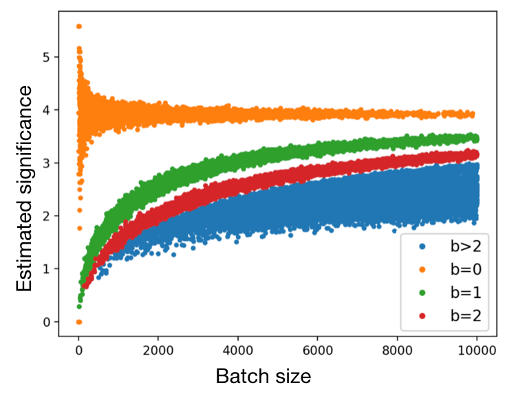
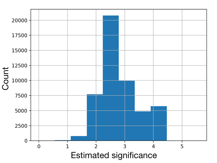
Figure 1: The $s/\sqrt{s+b}$ approximation of significance for a variety of batch sizes. Each batch is randomly sampled from the full set of events, with 10 points plotted for each batch size considered. A histogram of the significances from all of these attempted batch sizes is plotted on the right (b).

When optimising with $\ell_{Asimov}$, it was found that it would take many iterations of weight updates before the loss started minimising. In many cases the loss would not reduce below its initial value for a large number of epochs. This is due to the gradient of the Asimov estimate being small in the cases that $s$ is small with respect to $\sigma_{b}$. This can be resolved by carrying out a pretraining with $\ell_{s/\sqrt{s+b}}$, which has a higher gradient than $\ell_{Asimov}$ when $s/b$ is low. We find that a pretraining of $\sim 5$ epochs is typically enough to increase $s/b$ to a reasonable level, $\ell_{Asimov}$ can then be used to finish off the optimisation of the network.

5 Results

To demonstrate the performance of the loss functions described in Sec. 4, they are used to optimise a variety of simple neural networks that aim to discriminate signal from background in the toy SUSY analysis described in Sec. 2. All of the high and low level variables summarised in Tab. 1 are scaled so as to have a mean of 0 and a standard deviation of 1 and subsequently used as input features to the neural networks.

Dense networks with three distinct topologies are trained, one with a single hidden layer of 23 neurons, one with three hidden layers of 46 neurons and one with five hidden layers of 23 neurons. They all give the same qualitative results and have a similar performance on our simple toy problem. The results shown in this section are evaluated from the network with a single hidden layer, as it had the least sensitivity to overtraining and adequately demonstrates the performance.

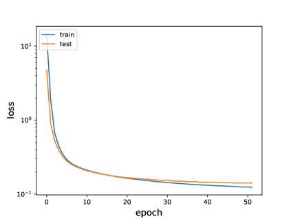
(a) Loss evolution

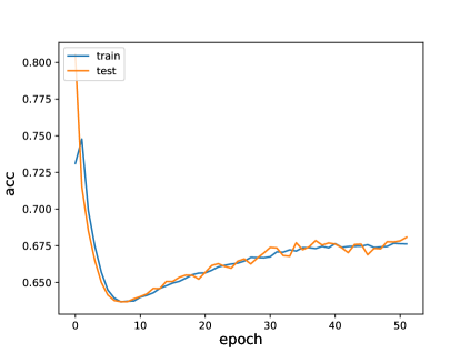
(b) Accuracy evolution

Figure 2: The evolution of the loss function (left) and accuracy of the model (right) for a single hidden layer neural network optimised with $\ell_{s/\sqrt{s+b}}$.

(a) Binary cross entropy

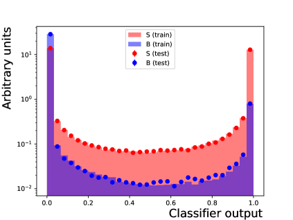
(b) $\ell_{s/\sqrt{s+b}}$

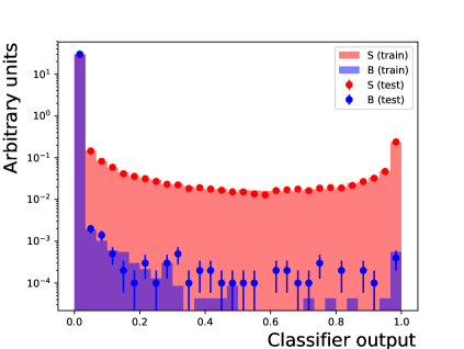
(c) $\ell_{Asimov}$

Figure 3: Histograms of the classifier outputs for the testing and training datasets of the value of the output neuron for single layer neural networks that are optimised with the three different loss functions. Both signal and background events have an equal weight.

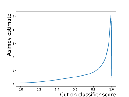
(a) Binary cross entropy

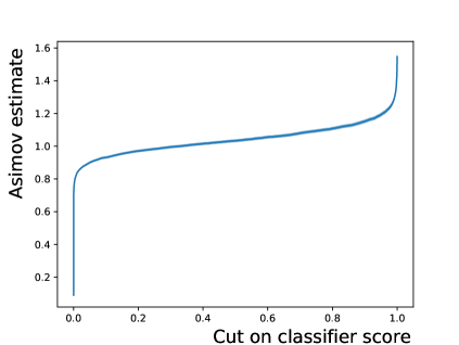
(b) $\ell_{s/\sqrt{s+b}}$

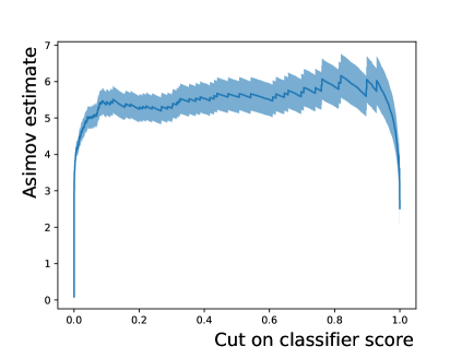
(c) $\ell_{Asimov}$

Figure 4: The Asimov estimate of significance with a $50\%$ systematic uncertainty on the background as a function of classifier cut for the one layer network trained with the three different loss functions. This is calculated for the compressed SUSY mass point. A $\pm 1\sigma$ error band of the estimate based on the simulation statistics is included in light blue. The significance is calculated with both signal and background events weighted to reflect the number of expected events observed in $30$ fb^-1 of $14$ TeV proton-proton collisions.

Loss	$Z_{A}(\sigma_{b}/b=0.1)$			$Z_{A}(\sigma_{b}/b=0.3)$			$Z_{A}(\sigma_{b}/b=0.5)$
	$s$	$b$	$\sigma$	$s$	$b$	$\sigma$	$s$	$b$	$\sigma$
Uncompressed model, $m_{stop}=900\,\text{GeV}$, $m_{LSP}=100\,\text{GeV}$
Cross entropy	$8.7$	$1.7$	$4.5\pm 0.3$	$7.7$	$1.2$	$4.0\pm 0.3$	$7.7$	$1.2$	$3.5\pm 0.3$
$\ell_{s/\sqrt{s+b}}$	$7.7$	$1.3$	$4.3\pm 0.3$	$7.7$	$1.3$	$3.9\pm 0.3$	$7.7$	$1.3$	$3.4\pm 0.3$
$\ell_{Asimov}$	$6.6$	$1.6$	$3.6\pm 0.2$	$3.5$	$0.1$	$4.0\pm 0.5$	$3.3$	$0.1$	$4.2\pm 0.7$
Compressed model, $m_{stop}=600\,\text{GeV}$, $m_{LSP}=400\,\text{GeV}$
Cross entropy	$74.4$	$18.2$	$10.7\pm 0.3$	$44.0$	$7.7$	$6.8\pm 0.3$	$40.5$	$6.8$	$4.8\pm 0.3$
$\ell_{s/\sqrt{s+b}}$	$323$	$326$	$7.0\pm 0.1$	$323$	$326$	$2.56\pm 0.03$	$324$	$327$	$1.55\pm 0.02$
$\ell_{Asimov}$	$78.4$	$19.4$	$10.8\pm 0.3$	$25.9$	$3.2$	$6.8\pm 0.4$	$11.9$	$0.5$	$6.2\pm 0.6$

Table 2: The expected number of signal, $s$, and background, $b$, events that lead to the best significance, $\sigma$, gained with a classification of signal and background obtained with a cut on the output neuron of a single layer neural network optimised with the three different loss functions. $Z_{A}$ is calculated with a $10\%$,$30\%$ or $50\%$ systematic uncertainty on the background. The expected numbers are calculated given 30 fb^-1 of 14 TeV LHC data.

Optimisation is carried out with three different loss functions, $\ell_{s/\sqrt{s+b}}$, $\ell_{Asimov}$ (with a range of systematic errors tested, from $5$-$50\%$ of the background counts) and the binary cross entropy. The Adam optimisation algorithm is used to minimise the loss [22]. As discussed in Sec. 4, a size of 4096 is used for the new loss functions. A batch size of 128 was found to work well for the binary cross entropy and is used throughout the studies. Each of the networks are trained until the value of the loss function in the test data does not decrease for two epochs.

The evolution of $\ell_{s/\sqrt{s+b}}$ and accuracy as a function of epoch for the test and train datasets can be seen in Fig. 2. It is evident that the minimisation of the loss function does not directly correspond to a monotonic increase in the accuracy, as would be the case for the binary cross entropy. The reason for this can be clearly seen in Fig. 3, which shows the value of the output neuron for the test and train datasets, split into signal and background events. The new loss functions maintain the purity of the signal classification at the expense of signal events, which are misclassified as background. The binary cross entropy, however, puts equal weight into the correct classification of the signal and background. This allows the new loss functions to select regions of phase space that have a purer signal to background ratio when it is advantageous to the overall significance to do so.

The performance for the two separate SUSY mass points introduced in Sec. 2 are considered. A separate training is carried out for each loss function for both of the models. To evaluate their performance, the value of the output neuron for each network, the classifier score, is considered. Potential cuts on this score are scanned through, where all the events that have a score greater than a cut value are kept. After these cuts the Asimov estimates of the significance for a variety of systematic uncertainties are calculated. Plots for each loss function, showing the significances as a function of cut value for the compressed SUSY model with a systematic uncertainty of $50\%$ of the background counts, is displayed in Fig. 4. The maximum significances obtainable with this method, along with the expected number of signal and background events remaining after the chosen cut, for each of the loss function and SUSY models are presented in Tab. 2. The error on the Asimov estimate is calculated by propagating the Poisson uncertainty of the background and signal counts.

For the uncompressed model, all three of the loss functions perform similarly. In this case there are appreciable differences in the distributions of the input variables between the signal and background samples, but a low number of signal events expected. This results in a significance that is limited by the statistical uncertainty, rather than the systematic uncertainty. As there is no advantage to factoring in the systematic uncertainties in this case, each loss function manages to find an optimal solution. However, there is a difference in purity of the selected signal and background events for the different loss functions. The maximum value of $s/b$ for the binary cross entropy optimisation, as a function of cut on the classifier, is $\sim 6$, whereas when optimising with $\ell_{Asimov}$ an $s/b$ of $\sim 30$ is obtained. The optimisation of $\ell_{s/\sqrt{s+b}}$ also resulted in an $s/b$ of $\sim 6$. This suggests that when the optimisation is aware of the systematic error, there is pressure for it to select a different region of phase spaced with a higher purity of signal events.

When optimising the networks for the compressed model, there is a bigger difference in the performance. In this case the signal and background distributions are more similar, but the cross section is higher, so there is a larger number of signal events for the network to correctly classify. This makes the result much more sensitive to systematic uncertainties than statistical uncertainties. The only optimisation that is aware of the systematic uncertainty is the one with $\ell_{Asimov}$. This results in a better performance for this loss, especially when considering higher systematic uncertainties. This gain is due to optimisation with $\ell_{Asimov}$ resulting in a higher purity. The optimisation with $\ell_{s/\sqrt{s+b}}$ contains no information about the systematic uncertainty and performs most poorly, finding a maximum $s/b$ of only $\sim 1$. The binary cross entropy still performs well, but requires a cut on values of the classifier score very close to one, interpretable as a very high probability of signal event and low probability of a background event. One other noticeable feature of the new loss functions is that it is unnecessary to tune the cut on the classifier to gain the optimal performance, all cuts above $\sim 0.5$ perform well.

A similar study was carried out considering 300 fb^-1, rather than 30 fb^-1, of LHC data. In this case the improvement shown by $\ell_{Asimov}$ was starker, with a $9.9\pm 1.6~{}\sigma$ separation achieved with a systematic uncertainty of $50\%$. By comparison, the binary cross entropy achieved a $6.4\pm 0.7~{}\sigma$ separation.

6 Conclusions

In searches for new physics at particle colliders, analyses aim at maximising the statistical significance of signal events over the background in a given search region. Neural networks offer a powerful technique for classifying signal and background events and thus determining search regions. New loss functions that directly maximise two estimations of statistical significance, $s/\sqrt{s+b}$ and the Asimov estimate, have been introduced. The optimal batch size is required to be fairly large, $O(10^{3})$, to minimise statistical fluctuations on the estimation of the significance in the loss functions. When optimising with $\ell_{Asimov}$ it is also found that some pretraining with $\ell_{s/\sqrt{s+b}}$ results in a significant speed up of the optimisation time.

These strategies have been tested in a simulation of a SUSY search for direct stop production in $30$ fb^-1 of $14$ TeV proton-proton collisions at the LHC. The optimisation with $\ell_{Asimov}$ has been demonstrated to select signal events with a higher purity than the standard loss function for neural network classification tasks, the binary cross entropy. This can result in a better discovery significance especially in models that are dominated by systematic uncertainties.

This toy study provides a proof of principle of the loss functions described in this paper, future studies will be carried out to determine their usefulness in a more realistic analysis scenario.

Examples of an implementation of the loss functions with the Keras python library [23] can be found in the GitHub repository containing the code used for this study.

References

- [1] P. Ramond, “Dual theory for free fermions,” Phys. Rev. D 3 (1971) 2415.
- [2] Y. A. Golfand and E. P. Likhtman, “Extension of the algebra of Poincaré group generators and violation of P invariance,” JETP Lett. 13 (1971) 323.
- [3] A. Neveu and J. H. Schwarz, “Factorizable dual model of pions,” Nucl. Phys. B 31 (1971) 86.
- [4] D. V. Volkov and V. P. Akulov, “Possible universal neutrino interaction,” JETP Lett. 16 (1972) 438.
- [5] J. Wess and B. Zumino, “A Lagrangian model invariant under supergauge transformations,” Phys. Lett. B 49 (1974) 52.
- [6] J. Wess and B. Zumino, “Supergauge transformations in four dimensions,” Nucl. Phys. B 70 (1974) 39.
- [7] P. Fayet, “Supergauge invariant extension of the Higgs mechanism and a model for the electron and its neutrino,” Nucl. Phys. B 90 (1975) 104.
- [8] H. P. Nilles, “Supersymmetry, supergravity and particle physics,” Phys. Rep. 110 (1984) 1.
- [9] P. Baldi, P. Sadowski, and D. Whiteson, “Searching for Exotic Particles in High-Energy Physics with Deep Learning,” Nature Commun. 5 (2014) 4308, arXiv:1402.4735 [hep-ph].
- [10] C. Borschensky, M. Krämer, A. Kulesza, M. Mangano, S. Padhi, T. Plehn, and X. Portell, “Squark and gluino production cross sections in pp collisions at = 13, 14, 33 and 100 TeV,” Eur. Phys. J. C74 no. 12, (2014) 3174, arXiv:1407.5066 [hep-ph].
- [11] J. M. Campbell and R. K. Ellis, “MCFM for the Tevatron and the LHC,” Nucl. Phys. Proc. Suppl. 205-206 (2010) 10, arXiv:1007.3492 [hep-ph].
- [12] P. M. Nadolsky, H.-L. Lai, Q.-H. Cao, J. Huston, J. Pumplin, D. Stump, W.-K. Tung, and C. P. Yuan, “Implications of CTEQ global analysis for collider observables,” Phys. Rev. D78 (2008) 013004, arXiv:0802.0007 [hep-ph].
- [13] T. Sjöstrand, S. Ask, J. R. Christiansen, R. Corke, N. Desai, P. Ilten, S. Mrenna, S. Prestel, C. O. Rasmussen, and P. Z. Skands, “An Introduction to PYTHIA 8.2,” Comput. Phys. Commun. 191 (2015) 159–177, arXiv:1410.3012 [hep-ph].
- [14] S. M. T. Sjöstrand and P. Skands, “PYTHIA 6.4 Physics and Manual,” JHEP 0605 (2006) 026, arXiv:hep-ph/0603175 [hep-ph].
- [15] J. de Favereau, C. Delaere, P. Demin, A. Giammanco, V. Lemaitre, A. Mertens, and M. Selvaggi, “DELPHES 3, A modular framework for fast simulation of a generic collider experiment,” JHEP 02 (2014) 057, arXiv:1307.6346 [hep-ex].
- [16] M. Cacciari, G. P. Salam, and G. Soyez, “The Anti-k(t) jet clustering algorithm,” JHEP 04 (2008) 063, arXiv:0802.1189 [hep-ph].
- [17] M. O. Sahin, D. Krücker, and I. A. Melzer-Pellmann, “Performance and optimization of support vector machines in high-energy physics classification problems,” Nucl. Instrum. Meth. A838 (2016) 137, arXiv:1601.02809 [hep-ex].
- [18] J. G. Yang Bai, Hsin-Chia Cheng and J. Gu, “Stop the top background of the stop search,” arXiv:1203.4813 [hep-ph].
- [19] A. P. Bradley, “The use of the area under the ROC curve in the evaluation of machine learning algorithms,” Pattern Recognition 30 no. 7, (1997) 1145–1159. http://dx.doi.org/10.1016/s0031-3203(96)00142-2.
- [20] K. P. Murphy, Machine learning - a probabilistic perspective. MIT Press, 2012.
- [21] G. Cowan, K. Cranmer, E. Gross, and O. Vitells, “Asymptotic formulae for likelihood-based tests of new physics,” European Physical Journal C 71 (Feb., 2011) 1554, arXiv:1007.1727 [physics.data-an].
- [22] D. P. Kingma and J. Ba, “Adam: A method for stochastic optimization,” CoRR abs/1412.6980 (2014) , arXiv:1412.6980. http://arxiv.org/abs/1412.6980.
- [23] F. Chollet et al., “Keras.” https://keras.io, 2015.