Adaptive BEM with inexact PCG solver
yields almost optimal computational costs

Thomas Führer Pontificia Universidad de Católica, Facultad de Matemáticas, Vickuña Mackenna 4860, Santiago, Chile tofuhrer@mat.uc.cl Alexander Haberl Dirk Praetorius  and  Stefan Schimanko TU Wien, Institute for Analysis and Scientific Computing, Wiedner Hauptstr. 8–10/E101/4, 1040 Wien, Austria { alexander.haberl , dirk.praetorius } @asc.tuwien.ac.at stefan.schimanko@asc.tuwien.ac.at (corresponding author)
Abstract.

We consider the preconditioned conjugate gradient method (PCG) with optimal preconditioner in the frame of the boundary element method (BEM) for elliptic first-kind integral equations. Our adaptive algorithm steers the termination of PCG as well as the local mesh-refinement. Besides convergence with optimal algebraic rates, we also prove almost optimal computational complexity. In particular, we provide an additive Schwarz preconditioner which can be computed in linear complexity and which is optimal in the sense that the condition numbers of the preconditioned systems are uniformly bounded. As model problem serves the 2D or 3D Laplace operator and the associated weakly-singular integral equation with energy space H~1/2(Γ)superscript~𝐻12Γ\widetilde{H}^{-1/2}(\Gamma). The main results also hold for the hyper-singular integral equation with energy space H1/2(Γ)superscript𝐻12ΓH^{1/2}(\Gamma).

Acknowledgement. The authors thankfully acknowledge the support by the Austrian Science Fund (FWF) through grant P27005 (AH, DP, SS) as well as grant F65 (DP) and by CONICYT through FONDECYT project P11170050 (TF)

1. Introduction

1.1. Model problem

Let ΩdΩsuperscript𝑑\Omega\subset\mathbb{R}^{d} with d=2,3𝑑23d=2,3 be a bounded Lipschitz domain with polyhedral boundary ΩΩ\partial\Omega. Let ΓΩΓΩ\Gamma\subseteq\partial\Omega be a (relatively) open and connected subset. Given f:Γ:𝑓Γf:\Gamma\to\mathbb{R}, we seek the density ϕ:Γ:superscriptitalic-ϕΓ\phi^{\star}\colon\Gamma\rightarrow\mathbb{R} of the weakly-singular integral equation

(1) (Vϕ)(x):=ΓG(xy)ϕ(y)dy=f(x)for all xΓ,formulae-sequenceassign𝑉superscriptitalic-ϕ𝑥subscriptΓ𝐺𝑥𝑦superscriptitalic-ϕ𝑦differential-d𝑦𝑓𝑥for all 𝑥Γ\displaystyle(V\phi^{\star})(x):=\int_{\Gamma}G(x-y)\phi^{\star}(y)\,{\rm d}y=f(x)\quad\text{for all }x\in\Gamma,

where G()𝐺G(\cdot) denotes the fundamental solution of the Laplace operator, i.e.,

(2) G(z)=12πlog|z|for d=2resp.G(z)=14π1|z|for d=3.formulae-sequence𝐺𝑧12𝜋𝑧formulae-sequencefor 𝑑2resp.formulae-sequence𝐺𝑧14𝜋1𝑧for 𝑑3\displaystyle G(z)=-\frac{1}{2\pi}\,\log|z|\quad\text{for }d=2\quad\text{resp.}\quad G(z)=\frac{1}{4\pi}\,\frac{1}{|z|}\quad\text{for }d=3.

Given a triangulation 𝒯subscript𝒯\mathcal{T}_{\bullet} of ΓΓ\Gamma, we employ a lowest-order Galerkin boundary element method (BEM) to compute a 𝒯subscript𝒯\mathcal{T}_{\bullet}-piecewise constant function ϕ𝒫0(𝒯)superscriptsubscriptitalic-ϕsuperscript𝒫0subscript𝒯\phi_{\bullet}^{\star}\in\mathcal{P}^{0}(\mathcal{T}_{\bullet}) such that

(3) Γ(Vϕ)(x)ψ(x)dx=Γf(x)ψ(x)dxfor all ψ𝒫0(𝒯).formulae-sequencesubscriptΓ𝑉superscriptsubscriptitalic-ϕ𝑥subscript𝜓𝑥differential-d𝑥subscriptΓ𝑓𝑥subscript𝜓𝑥differential-d𝑥for all subscript𝜓superscript𝒫0subscript𝒯\displaystyle\int_{\Gamma}(V\phi_{\bullet}^{\star})(x)\,\psi_{\bullet}(x)\,{\rm d}x=\int_{\Gamma}f(x)\,\psi_{\bullet}(x)\,{\rm d}x\quad\text{for all }\psi_{\bullet}\in\mathcal{P}^{0}(\mathcal{T}_{\bullet}).

With the numbering 𝒯={T1,,TN}subscript𝒯subscript𝑇1subscript𝑇𝑁\mathcal{T}_{\bullet}=\{T_{1},\dots,T_{N}\}, consider the standard basis {χ,j:j=1,,N}conditional-setsubscript𝜒𝑗𝑗1𝑁\big{\{}\chi_{\bullet,j}\,:\,j=1,\dots,N\big{\}} of 𝒫0(𝒯)superscript𝒫0subscript𝒯\mathcal{P}^{0}(\mathcal{T}_{\bullet}) consisting of characteristic functions χ,jsubscript𝜒𝑗\chi_{\bullet,j} of Tj𝒯subscript𝑇𝑗subscript𝒯T_{j}\in\mathcal{T}_{\bullet}. We make the ansatz

(4) ϕ=k=1N𝒙[k]χ,kwith coefficient vector 𝒙=(𝒙[1],,𝒙[N])N.formulae-sequencesuperscriptsubscriptitalic-ϕsuperscriptsubscript𝑘1𝑁superscriptsubscript𝒙delimited-[]𝑘subscript𝜒𝑘with coefficient vector superscriptsubscript𝒙superscriptsubscript𝒙delimited-[]1superscriptsubscript𝒙delimited-[]𝑁superscript𝑁\displaystyle\phi_{\bullet}^{\star}=\sum_{k=1}^{N}\boldsymbol{x}_{\bullet}^{\star}[k]\,\chi_{\bullet,k}\quad\text{with coefficient vector }\boldsymbol{x}_{\bullet}^{\star}=(\boldsymbol{x}_{\bullet}^{\star}[1],\dots,\boldsymbol{x}_{\bullet}^{\star}[N])\in\mathbb{R}^{N}.

Then, the Galerkin formulation (3) is equivalent to the linear system

(5) 𝑨𝒙=𝒃 with 𝑨[j,k]:=Tj(Vχ,k)(x)dx,𝒃[j]:=Tjf(x)dx,formulae-sequencesubscript𝑨superscriptsubscript𝒙subscript𝒃 with subscript𝑨𝑗𝑘assignsubscriptsubscript𝑇𝑗𝑉subscript𝜒𝑘𝑥differential-d𝑥assignsubscript𝒃delimited-[]𝑗subscriptsubscript𝑇𝑗𝑓𝑥differential-d𝑥\displaystyle\boldsymbol{A}_{\bullet}\boldsymbol{x}_{\bullet}^{\star}=\boldsymbol{b}_{\bullet}\text{\ \ with\ \ }\boldsymbol{A}_{\bullet}[j,k]:=\int_{T_{j}}(V\chi_{\bullet,k})(x)\,{\rm d}x,\quad\boldsymbol{b}_{\bullet}[j]:=\int_{T_{j}}f(x)\,{\rm d}x,

where the matrix 𝑨N×Nsubscript𝑨superscript𝑁𝑁\boldsymbol{A}_{\bullet}\in\mathbb{R}^{N\times N} is positive definite and symmetric. For a given initial triangulation 𝒯0subscript𝒯0\mathcal{T}_{0}, we consider an adaptive mesh-refinement strategy of the type

(6) solveestimatemarkrefine𝑠𝑜𝑙𝑣𝑒𝑒𝑠𝑡𝑖𝑚𝑎𝑡𝑒𝑚𝑎𝑟𝑘𝑟𝑒𝑓𝑖𝑛𝑒\displaystyle\boxed{~{}solve~{}}\longrightarrow\boxed{~{}estimate~{}}\longrightarrow\boxed{~{}mark~{}}\longrightarrow\boxed{~{}refine~{}}

which generates a sequence 𝒯subscript𝒯\mathcal{T}_{\ell} of successively refined triangulations 𝒯subscript𝒯\mathcal{T}_{\ell} for all 0subscript0\ell\in\mathbb{N}_{0}. We note that the condition number of the Galerkin matrix 𝑨subscript𝑨\boldsymbol{A}_{\ell} from (5) depends on the number of elements of 𝒯subscript𝒯\mathcal{T}_{\ell}, as well as the minimal and maximal diameter. Therefore, the step solve𝑠𝑜𝑙𝑣𝑒~{}solve~{} requires an efficient preconditioner as well as an appropriate iterative solver.

1.2. State of the art

In the last decade, the mathematical understanding of adaptive mesh-refinement has matured. We refer to [Dör96, MNS00, BDD04, Ste07, CKNS08, FFP14] for some milestones for adaptive finite element methods for second-order linear elliptic equations, [Gan13, FKMP13, FFK+14, FFK+15, AFF+17] for adaptive BEM, and [CFPP14] for a general framework of rate-optimality of adaptive mesh-refining algorithms. The interplay between adaptive mesh-refinement, optimal convergence rates, and inexact solvers has been addressed and analyzed for adaptive FEM for linear problems in [Ste07, ALMS13, AGL13], for eigenvalue problems in [CG12], and recently also for strongly monotone nonlinearities in [GHPS17]. In particular, all available results for adaptive BEM [Gan13, FKMP13, FFK+14, FFK+15, AFF+17] assume that the Galerkin system (5) is solved exactly. Instead, the present work analyzes an adaptive algorithm which steers both, the local mesh-refinement and the iterations of the PCG algorithm.

In principle, it is known [CFPP14, Section 7] that convergence and optimal convergence rates are preserved if the linear system is solved inexactly, but with sufficient accuracy. The purpose of this work is to guarantee the latter by incorporating an appropriate stopping criterion for the PCG solver into the adaptive algorithm. Moreover, to prove that the proposed algorithm does not only lead to optimal algebraic convergence rates, but also to (almost) optimal computational costs, we provide an appropriate symmetric and positive definite preconditioner 𝑷N×Nsubscript𝑷superscript𝑁𝑁\boldsymbol{P}_{\ell}\in\mathbb{R}^{N\times N} such that

  • \bullet

    first, the matrix-vector products with 𝑷1superscriptsubscript𝑷1\boldsymbol{P}_{\ell}^{-1} can be computed at linear cost;

  • \bullet

    second, the system matrix 𝑷1/2𝑨𝑷1/2subscriptsuperscript𝑷12subscript𝑨superscriptsubscript𝑷12\boldsymbol{P}^{-1/2}_{\ell}\boldsymbol{A}_{\ell}\boldsymbol{P}_{\ell}^{-1/2} of the preconditioned linear system

    (7) 𝑷1/2𝑨𝑷1/2𝒙~=𝑷1/2𝒃subscriptsuperscript𝑷12subscript𝑨superscriptsubscript𝑷12superscriptsubscript~𝒙superscriptsubscript𝑷12subscript𝒃\displaystyle\boldsymbol{P}^{-1/2}_{\ell}\boldsymbol{A}_{\ell}\boldsymbol{P}_{\ell}^{-1/2}\widetilde{\boldsymbol{x}}_{\ell}^{\star}=\boldsymbol{P}_{\ell}^{-1/2}\boldsymbol{b}_{\ell}

    has a uniformly bounded condition number which is independent of 𝒯subscript𝒯\mathcal{T}_{\ell}.

Then, 𝒙=𝑷1/2𝒙~superscriptsubscript𝒙superscriptsubscript𝑷12superscriptsubscript~𝒙\boldsymbol{x}_{\ell}^{\star}=\boldsymbol{P}_{\ell}^{-1/2}\widetilde{\boldsymbol{x}}_{\ell}^{\star} solves the original system (5). To that end, we exploit the multilevel structure of adaptively generated meshes in the framework of adaptive Schwarz methods. For hyper-singular integral equations, such a multilevel additive Schwarz preconditioner has been proposed and analyzed in [FFPS17a, FMPR15] for d=2,3𝑑23d=2,3 and for weakly-singular integral equations in [FFPS17b] for d=2𝑑2d=2. In particular, the present work closes this gap by analyzing an optimal additive Schwarz preconditioner for weakly-singular integral equations for d=3𝑑3d=3. We note that the proofs of [FFPS17a, FFPS17b] do not transfer to weakly-singular integral equations for d=3𝑑3d=3. Instead, we build on recent results for finite element discretizations [HWZ12, AGS16] which are then transferred to the present BEM setting by use of an abstract concept from [Osw99].

1.3. Outline and main results

Section 2 introduces the functional analytic framework and fixes the necessary notation. Section 3 states our main results. In Section 3.1, we define a local multilevel additive Schwarz preconditioner (24) for a sequence of locally refined meshes. Theorem 3.1 states that the 2subscript2\ell_{2}-condition number of the preconditioned systems is uniformly bounded for all these meshes, i.e., the preconditioner is optimal. In Section 3.2, we first state our adaptive algorithm which steers the local mesh-refinement as well as the stopping of the PCG iteration (Algorithm 3.2). Theorem 3.2 proves

  • \bullet

    that the overall error in the energy norm can be controlled a posteriori,

  • \bullet

    that the quasi-error (which consists of energy norm error plus error estimator) is linearly convergent in each step of the adaptive algorithm (i.e., independent of whether the algorithm decides for local mesh-refinement or for one step of the PCG iteration),

  • \bullet

    that the quasi-error even decays with optimal rate (i.e., with each possible algebraic rate) with respect to the degrees of freedom, i.e., Algorithm 3.2 is rate optimal in the sense of, e.g., [Ste07, CKNS08, FKMP13, CFPP14].

Finally, Section 3.3 considers the computational costs. Under realistic assumptions on the treatment of the arising discrete integral operators, Corollary 3.3 states that the quasi-error converges at almost optimal rate (i.e., with rate sε𝑠𝜀s-\varepsilon for any ε>0𝜀0\varepsilon>0 if rate s>0𝑠0s>0 is possible for the exact Galerkin solution) with respect to computational costs, i.e., Algorithm 3.2 requires almost optimal computational time. Section 4 underpins our theoretical findings by some 2D and 3D experiments. The proof of Theorem 3.1 is given in Section 5, the proofs of Theorem 3.2 and Corollary 3.3 are given in Section 6. The final Section 7 shows that our main results also apply to the hyper-singular integral equation.

2. Preliminaries and notation

2.1. Functional analytic setting

We briefly recall the most important facts and refer to [McL00] for further details and proofs. With the Sobolev space Hα(Ω)superscript𝐻𝛼ΩH^{\alpha}(\partial\Omega) defined as in [McL00] for 0α10𝛼10\leq\alpha\leq 1, let Hα(Γ):={v|Γ:vHα(Ω)}H^{\alpha}(\Gamma):=\big{\{}v|_{\Gamma}\,:\,v\in H^{\alpha}(\partial\Omega)\big{\}} be associated with the natural quotient norm. Let H~α(Γ)superscript~𝐻𝛼Γ\widetilde{H}^{-\alpha}(\Gamma) be the dual space of Hα(Γ)superscript𝐻𝛼ΓH^{\alpha}(\Gamma) with respect to the extended L2(Γ)superscript𝐿2ΓL^{2}(\Gamma) scalar product ψ,f=Γψ(x)f(x)dx𝜓𝑓subscriptΓ𝜓𝑥𝑓𝑥differential-d𝑥\langle\psi\,,\,f\rangle=\int_{\Gamma}\psi(x)\,f(x)\,{\rm d}x. Then, the single-layer potential V𝑉V from (1) gives rise to a bounded linear operator V:H~1/2+s(Γ)H1/2+s(Γ):𝑉superscript~𝐻12𝑠Γsuperscript𝐻12𝑠ΓV:\widetilde{H}^{-1/2+s}(\Gamma)\to H^{1/2+s}(\Gamma) for all 1/2s1/212𝑠12-1/2\leq s\leq 1/2 which is even an isomorphism for 1/2<s<1/212𝑠12-1/2<s<1/2. For d=2𝑑2d=2, the latter requires diam(Ω)<1diamΩ1{\rm diam}(\Omega)<1 which can always be ensured by scaling of ΩΩ\Omega. For s=0𝑠0s=0, the operator V𝑉V is even symmetric and elliptic, i.e.,

(8) ϕ,ψ:=Γ(Vϕ)(x)ψ(x)dxfor all ϕ,ψH~1/2(Γ)assigndelimited-⟨⟩italic-ϕ𝜓subscriptΓ𝑉italic-ϕ𝑥𝜓𝑥differential-d𝑥for all ϕ,ψH~1/2(Γ)\displaystyle\langle\!\!\langle\phi\,,\,\psi\rangle\!\!\rangle:=\int_{\Gamma}(V\phi)(x)\,\psi(x)\,{\rm d}x\qquad\textrm{for all $\phi,\psi\in\widetilde{H}^{-1/2}(\Gamma)$}

defines a scalar product and |ϕ|2:=ϕ,ϕassignsuperscriptnormitalic-ϕ2delimited-⟨⟩italic-ϕitalic-ϕ|\!|\!|\,\phi\,|\!|\!|^{2}:=\langle\!\!\langle\phi\,,\,\phi\rangle\!\!\rangle is an equivalent norm on H~1/2(Γ)superscript~𝐻12Γ\widetilde{H}^{-1/2}(\Gamma). For a given right-hand side fH1/2(Γ)𝑓superscript𝐻12Γf\in H^{1/2}(\Gamma), the weakly-singular integral equation (1) can thus equivalently be reformulated as

(9) ϕ,ψ=f,ψ for all ψH~1/2(Γ).formulae-sequencedelimited-⟨⟩superscriptitalic-ϕ𝜓𝑓𝜓 for all 𝜓superscript~𝐻12Γ\displaystyle\langle\!\!\langle\phi^{\star}\,,\,\psi\rangle\!\!\rangle=\langle f\,,\,\psi\rangle\quad\text{ for all }\psi\in\widetilde{H}^{-1/2}(\Gamma).

In particular, the Lax–Milgram theorem proves existence and uniqueness of the solution ϕH~1/2(Γ)superscriptitalic-ϕsuperscript~𝐻12Γ\phi^{\star}\in\widetilde{H}^{-1/2}(\Gamma) to (9).

2.2. Boundary element method (BEM)

Given a mesh 𝒯subscript𝒯\mathcal{T}_{\bullet} of ΓΓ\Gamma, let

(10) 𝒫0(𝒯):={ψ:Γ:T𝒯ψ|T is constant}assignsuperscript𝒫0subscript𝒯conditional-setsubscript𝜓:Γfor-all𝑇subscript𝒯evaluated-atsubscript𝜓𝑇 is constant\displaystyle\mathcal{P}^{0}(\mathcal{T}_{\bullet}):=\big{\{}\psi_{\bullet}:\Gamma\to\mathbb{R}\,:\,\forall T\in\mathcal{T}_{\bullet}\quad\psi_{\bullet}|_{T}\text{ is constant}\big{\}}

be the space of 𝒯subscript𝒯\mathcal{T}_{\bullet}-piecewise constant functions. Note that 𝒫0(𝒯)L2(Γ)H~1/2(Γ)superscript𝒫0subscript𝒯superscript𝐿2Γsuperscript~𝐻12Γ\mathcal{P}^{0}(\mathcal{T}_{\bullet})\subset L^{2}(\Gamma)\subset\widetilde{H}^{-1/2}(\Gamma). The Galerkin formulation (3) can be reformulated as

(11) ϕ,ψ=f,ψfor all ψ𝒫0(𝒯).formulae-sequencedelimited-⟨⟩superscriptsubscriptitalic-ϕsubscript𝜓𝑓subscript𝜓for all subscript𝜓superscript𝒫0subscript𝒯\displaystyle\langle\!\!\langle\phi_{\bullet}^{\star}\,,\,\psi_{\bullet}\rangle\!\!\rangle=\langle f\,,\,\psi_{\bullet}\rangle\quad\text{for all }\psi_{\bullet}\in\mathcal{P}^{0}(\mathcal{T}_{\bullet}).

Therefore, the Lax–Milgram theorem proves existence and uniqueness of the discrete solution ϕ𝒫0(𝒯)superscriptsubscriptitalic-ϕsuperscript𝒫0subscript𝒯\phi_{\bullet}^{\star}\in\mathcal{P}^{0}(\mathcal{T}_{\bullet}).

Refer to caption
Refer to caption
Refer to caption
Figure 1. For newest vertex bisection (NVB) in 2D, each triangle T𝒯𝑇𝒯T\in\mathcal{T} has one reference edge, indicated by the double line (left). Bisection of T𝑇T is achieved by halving the reference edge (middle). The reference edges of the sons are always opposite to the new vertex. Recursive application of this refinement rule leads to conforming triangulations.

2.3. Mesh-refinement for 2D BEM

For d=2𝑑2d=2, a mesh 𝒯subscript𝒯\mathcal{T}_{\bullet} of ΓΓ\Gamma is a partition into non-degenerate compact line segments. It is called γ𝛾\gamma-shape regular, if

(12) max{hT/hT:T,T𝒯 with TT}γ.:subscript𝑇subscriptsuperscript𝑇𝑇superscript𝑇subscript𝒯 with 𝑇superscript𝑇𝛾\displaystyle\max\big{\{}h_{T}/h_{T^{\prime}}\,:\,T,T^{\prime}\in\mathcal{T}_{\bullet}\text{ with }T\cap T^{\prime}\neq\emptyset\big{\}}\leq\gamma.

Here, hT:=diam(T)>0assignsubscript𝑇diam𝑇0h_{T}:={\rm diam}(T)>0 denotes the Euclidean diameter of T𝑇T, i.e., the length of the line segment.

We employ the extended bisection algorithm from [AFF+13]. For a mesh 𝒯subscript𝒯\mathcal{T}_{\bullet} and 𝒯subscriptsubscript𝒯\mathcal{M}_{\bullet}\subseteq\mathcal{T}_{\bullet}, let 𝒯:=refine(𝒯,)assignsubscript𝒯refinesubscript𝒯subscript\mathcal{T}_{\circ}:={\rm refine}(\mathcal{T}_{\bullet},\mathcal{M}_{\bullet}) be the coarsest mesh such that all marked elements T𝑇subscriptT\in\mathcal{M}_{\bullet} have been refined, i.e., 𝒯\𝒯subscript\subscript𝒯subscript𝒯\mathcal{M}_{\bullet}\subseteq\mathcal{T}_{\bullet}\backslash\mathcal{T}_{\circ}. We write 𝒯refine(𝒯)subscript𝒯refinesubscript𝒯\mathcal{T}_{\circ}\in{\rm refine}(\mathcal{T}_{\bullet}), if there exists n0𝑛subscript0n\in\mathbb{N}_{0}, conforming triangulations 𝒯0,,𝒯nsubscript𝒯0subscript𝒯𝑛\mathcal{T}_{0},\dots,\mathcal{T}_{n} and corresponding sets of marked elements j𝒯jsubscript𝑗subscript𝒯𝑗\mathcal{M}_{j}\subseteq\mathcal{T}_{j} such that

  • \bullet

    𝒯=𝒯0subscript𝒯subscript𝒯0\mathcal{T}_{\bullet}=\mathcal{T}_{0},

  • \bullet

    𝒯j+1=refine(𝒯j,j)subscript𝒯𝑗1refinesubscript𝒯𝑗subscript𝑗\mathcal{T}_{j+1}={\rm refine}(\mathcal{T}_{j},\mathcal{M}_{j}) for all j=0,,n1𝑗0𝑛1j=0,\dots,n-1,

  • \bullet

    𝒯=𝒯nsubscript𝒯subscript𝒯𝑛\mathcal{T}_{\circ}=\mathcal{T}_{n},

i.e., 𝒯subscript𝒯\mathcal{T}_{\circ} is obtained from 𝒯subscript𝒯\mathcal{T}_{\bullet} by finitely many steps of refinement. Note that the bisection algorithm from [AFF+13] guarantees, in particular, that all 𝒯refine(𝒯)subscript𝒯refinesubscript𝒯\mathcal{T}_{\circ}\in{\rm refine}(\mathcal{T}_{\bullet}) are uniformly γ𝛾\gamma-shape regular, where γ𝛾\gamma depends only on 𝒯subscript𝒯\mathcal{T}_{\bullet}.

2.4. Mesh-refinement for 3D BEM

For d=3𝑑3d=3, a mesh 𝒯subscript𝒯\mathcal{T}_{\bullet} of ΓΓ\Gamma is a conforming triangulation into non-degenerate compact surface triangles. In particular, we avoid hanging nodes. To ease the presentation, we suppose that the elements T𝒯𝑇subscript𝒯T\in\mathcal{T}_{\bullet} are flat. The triangulation is called γ𝛾\gamma-shape regular, if

(13) maxT𝒯diam(T)hTγ.subscript𝑇subscript𝒯diam𝑇subscript𝑇𝛾\displaystyle\max_{T\in\mathcal{T}_{\bullet}}\frac{{\rm diam}(T)}{h_{T}}\leq\gamma.

Here, diam(T)diam𝑇{\rm diam}(T) denotes the Euclidean diameter of T𝑇T and hT:=|T|1/2assignsubscript𝑇superscript𝑇12h_{T}:=|T|^{1/2} with |T|𝑇|T| being the two-dimensional surface measure. Note that γ𝛾\gamma-shape regularity implies that hTdiam(T)γhTsubscript𝑇diam𝑇𝛾subscript𝑇h_{T}\leq{\rm diam}(T)\leq\gamma\,h_{T} and hence excludes anisotropic elements.

For 3D BEM, we employ 2D newest vertex bisection (NVB) to refine triangulations locally; see [Ste08, KPP13] for details on the refinement algorithm and Figure 1 for an illustration. For a mesh 𝒯subscript𝒯\mathcal{T}_{\bullet} and 𝒯subscriptsubscript𝒯\mathcal{M}_{\bullet}\subseteq\mathcal{T}_{\bullet}, we employ the same notation 𝒯:=refine(𝒯,)assignsubscript𝒯refinesubscript𝒯subscript\mathcal{T}_{\circ}:={\rm refine}(\mathcal{T}_{\bullet},\mathcal{M}_{\bullet}) resp. 𝒯refine(𝒯)subscript𝒯refinesubscript𝒯\mathcal{T}_{\circ}\in{\rm refine}(\mathcal{T}_{\bullet}) as for d=2𝑑2d=2.

2.5. A posteriori BEM error control

For ψ𝒫0(𝒯)subscript𝜓superscript𝒫0subscript𝒯\psi_{\bullet}\in\mathcal{P}^{0}(\mathcal{T}_{\bullet}) and 𝒰𝒯subscript𝒰subscript𝒯\mathcal{U}_{\bullet}\subseteq\mathcal{T}_{\bullet}, define

(14) η(𝒰,ψ)2:=T𝒰η(T,ψ)2,whereη(T,ψ)2:=hTΓ(fVψ)L2(T)2.formulae-sequenceassignsubscript𝜂superscriptsubscript𝒰subscript𝜓2subscript𝑇subscript𝒰subscript𝜂superscript𝑇subscript𝜓2whereassignsubscript𝜂superscript𝑇subscript𝜓2subscript𝑇superscriptsubscriptnormsubscriptΓ𝑓𝑉subscript𝜓superscript𝐿2𝑇2\displaystyle\eta_{\bullet}(\mathcal{U}_{\bullet},\psi_{\bullet})^{2}:=\sum_{T\in\mathcal{U}_{\bullet}}\eta_{\bullet}(T,\psi_{\bullet})^{2},\quad\text{where}\quad\eta_{\bullet}(T,\psi_{\bullet})^{2}:=h_{T}\,\|\nabla_{\Gamma}(f-V\psi_{\bullet})\|_{L^{2}(T)}^{2}.

Here Γ()subscriptΓ\nabla_{\Gamma}(\cdot) denotes the arclength derivative for d=2𝑑2d=2 resp. the surface gradient for d=3𝑑3d=3. To abbreviate notation, let η(ψ):=η(𝒯,ψ)assignsubscript𝜂subscript𝜓subscript𝜂subscript𝒯subscript𝜓\eta_{\bullet}(\psi_{\bullet}):=\eta_{\bullet}(\mathcal{T}_{\bullet},\psi_{\bullet}). If ψ=ϕsubscript𝜓superscriptsubscriptitalic-ϕ\psi_{\bullet}=\phi_{\bullet}^{\star} is the discrete solution to (11), then there holds the reliability estimate (i.e., the global upper bound)

(15) |ϕϕ|Crelη(ϕ),normsuperscriptitalic-ϕsuperscriptsubscriptitalic-ϕsubscript𝐶relsubscript𝜂superscriptsubscriptitalic-ϕ\displaystyle|\!|\!|\,\phi^{\star}-\phi_{\bullet}^{\star}\,|\!|\!|\leq C_{\rm rel}\,\eta_{\bullet}(\phi_{\bullet}^{\star}),

where Crel>0subscript𝐶rel0C_{\rm rel}>0 depends only on ΓΓ\Gamma and γ𝛾\gamma-shape regularity of 𝒯subscript𝒯\mathcal{T}_{\bullet}; see [CS95, Car97] for d=2𝑑2d=2 resp. [CMS01] for d=3𝑑3d=3. Provided that ϕL2(Γ)superscriptitalic-ϕsuperscript𝐿2Γ\phi^{\star}\in L^{2}(\Gamma), the following weak efficiency

(16) |ϕϕ|+η(ϕ)Ceffh1/2(ϕϕ)L2(Γ)normsuperscriptitalic-ϕsuperscriptsubscriptitalic-ϕsubscript𝜂superscriptsubscriptitalic-ϕsubscript𝐶effsubscriptnormsuperscriptsubscript12superscriptitalic-ϕsuperscriptsubscriptitalic-ϕsuperscript𝐿2Γ\displaystyle|\!|\!|\,\phi^{\star}-\phi_{\bullet}^{\star}\,|\!|\!|+\eta_{\bullet}(\phi_{\bullet}^{\star})\leq C_{\rm eff}\,\|h_{\bullet}^{1/2}\,(\phi^{\star}-\phi_{\bullet}^{\star})\|_{L^{2}(\Gamma)}

has recently been proved in [AFF+17], where Ceff>0subscript𝐶eff0C_{\rm eff}>0 depends only on ΓΓ\Gamma and γ𝛾\gamma-shape regulartiy of 𝒯subscript𝒯\mathcal{T}_{\bullet}. We note that the weighted L2superscript𝐿2L^{2}-norm on the right-hand side of (16) is only slightly stronger than ||||||H~1/2(Γ)|\!|\!|\,\cdot\,|\!|\!|\simeq\|\cdot\|_{\widetilde{H}^{-1/2}(\Gamma)}, so that one empirically observes η(ϕ)|ϕϕ|less-than-or-similar-tosubscript𝜂superscriptsubscriptitalic-ϕnormitalic-ϕsuperscriptsubscriptitalic-ϕ\eta_{\bullet}(\phi_{\bullet}^{\star})\lesssim|\!|\!|\,\phi-\phi_{\bullet}^{\star}\,|\!|\!| in practice, cf. [CS95, Car97, CMS01]. In certain situations (e.g., weakly-singular integral formulation of the interior 2D Dirichlet problem), one can rigorously prove the latter (strong) efficiency estimate up to higher-order data oscillations; see [AFF+13].

2.6. Preconditioned conjugate gradient method (PCG)

Suppose that 𝑷,𝑨N×Nsubscript𝑷subscript𝑨superscript𝑁𝑁\boldsymbol{P}_{\bullet},\boldsymbol{A}_{\bullet}\in\mathbb{R}^{N\times N} are symmetric and positive definite matrices. Given 𝒃Nsubscript𝒃superscript𝑁\boldsymbol{b}_{\bullet}\in\mathbb{R}^{N} and an initial guess 𝒙0subscript𝒙absent0\boldsymbol{x}_{\bullet 0}, PCG (see [GVL13, Algorithm 11.5.1]) aims to approximate the solution 𝒙Nsuperscriptsubscript𝒙superscript𝑁\boldsymbol{x}_{\bullet}^{\star}\in\mathbb{R}^{N} to (5). We note that each step of PCG has the following computational costs:

  • \bullet

    𝒪(N)𝒪𝑁\mathcal{O}(N) cost for vector operations (e.g., assignment, addition, scalar product),

  • \bullet

    computation of one matrix-vector product with 𝑨subscript𝑨\boldsymbol{A}_{\bullet},

  • \bullet

    computation of one matrix-vector product with 𝑷1superscriptsubscript𝑷1\boldsymbol{P}_{\bullet}^{-1}.

Let 𝒙~Nsuperscriptsubscript~𝒙superscript𝑁\widetilde{\boldsymbol{x}}_{\bullet}^{\star}\in\mathbb{R}^{N} be the solution to (7) and recall that 𝒙=𝑷1/2𝒙~superscriptsubscript𝒙superscriptsubscript𝑷12superscriptsubscript~𝒙\boldsymbol{x}_{\bullet}^{\star}=\boldsymbol{P}_{\bullet}^{-1/2}\widetilde{\boldsymbol{x}}_{\bullet}^{\star}. We note that PCG formally applies the conjugate gradient method (CG, see [GVL13, Algorithm 11.3.2]) for the matrix 𝑨~:=𝑷1/2𝑨𝑷1/2assignsubscript~𝑨superscriptsubscript𝑷12subscript𝑨superscriptsubscript𝑷12\widetilde{\boldsymbol{A}}_{\bullet}:=\boldsymbol{P}_{\bullet}^{-1/2}\boldsymbol{A}_{\bullet}\boldsymbol{P}_{\bullet}^{-1/2} and the right-hand side 𝒃~=𝑷1/2𝒃subscript~𝒃superscriptsubscript𝑷12subscript𝒃\widetilde{\boldsymbol{b}}_{\bullet}=\boldsymbol{P}_{\bullet}^{-1/2}\boldsymbol{b}_{\bullet}. The iterates 𝒙kNsubscript𝒙absent𝑘superscript𝑁\boldsymbol{x}_{\bullet k}\in\mathbb{R}^{N} of PCG (applied to 𝑷subscript𝑷\boldsymbol{P}_{\bullet}, 𝑨subscript𝑨\boldsymbol{A}_{\bullet}, 𝒃subscript𝒃\boldsymbol{b}_{\bullet}, and the initial guess 𝒙0subscript𝒙absent0\boldsymbol{x}_{\bullet 0}) and the iterates 𝒙~ksubscript~𝒙absent𝑘\widetilde{\boldsymbol{x}}_{\bullet k} of CG (applied to 𝑨~subscript~𝑨\widetilde{\boldsymbol{A}}_{\bullet}, 𝒃~subscript~𝒃\widetilde{\boldsymbol{b}}_{\bullet}, and the initial guess 𝒙~0:=𝑷1/2𝒙0assignsubscript~𝒙absent0superscriptsubscript𝑷12subscript𝒙absent0\widetilde{\boldsymbol{x}}_{\bullet 0}:=\boldsymbol{P}_{\bullet}^{1/2}\boldsymbol{x}_{\bullet 0}) are formally linked by

𝒙k=𝑷1/2𝒙~k;subscript𝒙absent𝑘superscriptsubscript𝑷12subscript~𝒙absent𝑘\displaystyle\boldsymbol{x}_{\bullet k}=\boldsymbol{P}_{\bullet}^{-1/2}\widetilde{\boldsymbol{x}}_{\bullet k};

see [GVL13, Section 11.5]. Moreover, direct computation proves that

(17) 𝒚~𝑨~2:=𝒚~𝑨~𝒚~=𝒚𝑨𝒚=:𝒚𝑨2for all 𝒚~N and 𝒚=𝑷1/2𝒚~.\displaystyle\|\widetilde{\boldsymbol{y}}_{\bullet}\|_{\widetilde{\boldsymbol{A}}_{\bullet}}^{2}:=\widetilde{\boldsymbol{y}}_{\bullet}\cdot\widetilde{\boldsymbol{A}}_{\bullet}\widetilde{\boldsymbol{y}}_{\bullet}=\boldsymbol{y}_{\bullet}\cdot\boldsymbol{A}_{\bullet}\boldsymbol{y}_{\bullet}=:\|\boldsymbol{y}_{\bullet}\|_{\boldsymbol{A}_{\bullet}}^{2}\quad\text{for all $\widetilde{\boldsymbol{y}}_{\bullet}\in\mathbb{R}^{N}$ and $\boldsymbol{y}_{\bullet}=\boldsymbol{P}_{\bullet}^{-1/2}\widetilde{\boldsymbol{y}}_{\bullet}$}.

Consequently, [GVL13, Theorem 11.3.3] for CG (applied to 𝑨~subscript~𝑨\widetilde{\boldsymbol{A}}_{\bullet}, 𝒃~subscript~𝒃\widetilde{\boldsymbol{b}}_{\bullet}, 𝒙~0subscript~𝒙absent0\widetilde{\boldsymbol{x}}_{\bullet 0}) yields the following lemma for PCG (which follows from the implicit steepest decent approach of CG).

   Lemma 1.  Let 𝐀,𝐏N×Nsubscript𝐀subscript𝐏superscript𝑁𝑁\boldsymbol{A}_{\bullet},\boldsymbol{P}_{\bullet}\in\mathbb{R}^{N\times N} be symmetric and positive definite, 𝐛Nsubscript𝐛superscript𝑁\boldsymbol{b}_{\bullet}\in\mathbb{R}^{N}, 𝐱:=𝐀1𝐛assignsuperscriptsubscript𝐱superscriptsubscript𝐀1subscript𝐛\boldsymbol{x}_{\bullet}^{\star}:=\boldsymbol{A}_{\bullet}^{-1}\boldsymbol{b}_{\bullet}, and 𝐱0Nsubscript𝐱absent0superscript𝑁\boldsymbol{x}_{\bullet 0}\in\mathbb{R}^{N}. Suppose the 2subscript2\ell_{2}-condition number estimate

(18) cond2(𝑷1/2𝑨𝑷1/2)Cpcg.subscriptcond2superscriptsubscript𝑷12subscript𝑨superscriptsubscript𝑷12subscript𝐶pcg\displaystyle{\rm cond}_{2}(\boldsymbol{P}_{\bullet}^{-1/2}\boldsymbol{A}_{\bullet}\boldsymbol{P}_{\bullet}^{-1/2})\leq C_{\rm pcg}.

Then, the iterates 𝐱ksubscript𝐱absent𝑘\boldsymbol{x}_{\bullet k} of the PCG algorithm satisfy the contraction property

(19) 𝒙𝒙(k+1)𝑨qpcg𝒙𝒙k𝑨for all k0,formulae-sequencesubscriptnormsuperscriptsubscript𝒙subscript𝒙absent𝑘1subscript𝑨subscript𝑞pcgsubscriptnormsuperscriptsubscript𝒙subscript𝒙absent𝑘subscript𝑨for all 𝑘subscript0\displaystyle\|\boldsymbol{x}_{\bullet}^{\star}-\boldsymbol{x}_{\bullet(k+1)}\|_{\boldsymbol{A}_{\bullet}}\leq q_{\rm pcg}\,\|\boldsymbol{x}_{\bullet}^{\star}-\boldsymbol{x}_{\bullet k}\|_{\boldsymbol{A}_{\bullet}}\quad\text{for all }k\in\mathbb{N}_{0},

where qpcg:=(11/Cpcg)1/2<1assignsubscript𝑞pcgsuperscript11subscript𝐶pcg121q_{\rm pcg}:=(1-1/C_{\rm pcg})^{1/2}<1.∎   

If the matrix 𝑨N×Nsubscript𝑨superscript𝑁𝑁\boldsymbol{A}_{\bullet}\in\mathbb{R}^{N\times N} stems from the Galerkin discretization (5) for 𝒯={T1,,TN}subscript𝒯subscript𝑇1subscript𝑇𝑁\mathcal{T}_{\bullet}=\{T_{1},\dots,T_{N}\}, there is a one-to-one correspondence of vectors 𝒚Nsubscript𝒚superscript𝑁\boldsymbol{y}_{\bullet}\in\mathbb{R}^{N} and discrete functions ψ𝒫0(𝒯)subscript𝜓superscript𝒫0subscript𝒯\psi_{\bullet}\in\mathcal{P}^{0}(\mathcal{T}_{\bullet}) via ψ=j=1N𝒚[j]χ,jsubscript𝜓superscriptsubscript𝑗1𝑁subscript𝒚delimited-[]𝑗subscript𝜒𝑗\psi_{\bullet}=\sum_{j=1}^{N}\boldsymbol{y}_{\bullet}[j]\,\chi_{\bullet,j}. Let ϕk𝒫0(𝒯)subscriptitalic-ϕabsent𝑘superscript𝒫0subscript𝒯\phi_{\bullet k}\in\mathcal{P}^{0}(\mathcal{T}_{\bullet}) denote the discrete function corresponding to the PCG iterate 𝒙kNsubscript𝒙absent𝑘superscript𝑁\boldsymbol{x}_{\bullet k}\in\mathbb{R}^{N}, while the Galerkin solution ϕ𝒫0(𝒯)superscriptsubscriptitalic-ϕsuperscript𝒫0subscript𝒯\phi_{\bullet}^{\star}\in\mathcal{P}^{0}(\mathcal{T}_{\bullet}) of (11) corresponds to 𝒙=𝑨1𝒃superscriptsubscript𝒙superscriptsubscript𝑨1subscript𝒃\boldsymbol{x}_{\bullet}^{\star}=\boldsymbol{A}_{\bullet}^{-1}\boldsymbol{b}_{\bullet}. We note the elementary identity

(20) |ϕϕk|2=(𝒙𝒙k)𝑨(𝒙𝒙k)=𝒙𝒙k𝑨2.superscriptnormsuperscriptsubscriptitalic-ϕsubscriptitalic-ϕabsent𝑘2superscriptsubscript𝒙subscript𝒙absent𝑘subscript𝑨superscriptsubscript𝒙subscript𝒙absent𝑘superscriptsubscriptnormsuperscriptsubscript𝒙subscript𝒙absent𝑘subscript𝑨2\displaystyle|\!|\!|\,\phi_{\bullet}^{\star}-\phi_{\bullet k}\,|\!|\!|^{2}=(\boldsymbol{x}_{\bullet}^{\star}-\boldsymbol{x}_{\bullet k})\cdot\boldsymbol{A}_{\bullet}(\boldsymbol{x}_{\bullet}^{\star}-\boldsymbol{x}_{\bullet k})=\|\boldsymbol{x}_{\bullet}^{\star}-\boldsymbol{x}_{\bullet k}\|_{\boldsymbol{A}_{\bullet}}^{2}.

2.7. Optimal preconditioners

We say that 𝑷subscript𝑷\boldsymbol{P}_{\bullet} is an optimal preconditioner, if Cpcg1subscript𝐶pcg1C_{\rm pcg}\geq 1 in the 2subscript2\ell_{2}-condition number estimate (18) depends only on γ𝛾\gamma-shape regularity of 𝒯subscript𝒯\mathcal{T}_{\bullet} and the initial mesh 𝒯0subscript𝒯0\mathcal{T}_{0} (and is hence essentially independent of the mesh 𝒯subscript𝒯\mathcal{T}_{\bullet}).

3. Main results

3.1. Optimal additive Schwarz preconditioner

In this work, we consider multilevel additive Schwarz preconditioners that build on the adaptive mesh-hierarchy.

Let subscript\mathcal{E}_{\bullet} denote the set of all nodes (d=2𝑑2d=2) resp. edges (d=3𝑑3d=3) of the mesh 𝒯subscript𝒯\mathcal{T}_{\bullet} which do not belong to the relative boundary ΓΓ\partial\Gamma. Only for Γ=ΩΓΩ\Gamma=\partial\Omega, subscript\mathcal{E}_{\bullet} contains all nodes resp. edges of 𝒯subscript𝒯\mathcal{T}_{\bullet}. For E𝐸subscriptE\in\mathcal{E}_{\bullet}, let T±𝒯superscript𝑇plus-or-minussubscript𝒯T^{\pm}\in\mathcal{T}_{\bullet} denote the two unique elements with T+T=Esuperscript𝑇superscript𝑇𝐸T^{+}\cap T^{-}=E. We define the Haar-type function φ,E𝒫0(𝒯)subscript𝜑𝐸superscript𝒫0subscript𝒯\varphi_{\bullet,E}\in\mathcal{P}^{0}(\mathcal{T}_{\bullet}) (associated to E𝐸subscriptE\in\mathcal{E}_{\bullet}) by

(21) φ,E|T:={±|E||T±|for T{T+,T},0else,assignevaluated-atsubscript𝜑𝐸𝑇casesplus-or-minus𝐸superscript𝑇plus-or-minusfor 𝑇superscript𝑇superscript𝑇0else\displaystyle\varphi_{\bullet,E}|_{T}:=\begin{cases}\pm\frac{|E|}{|T^{\pm}|}&\text{for }T\in\{T^{+},T^{-}\},\\ 0&\text{else},\end{cases}

where |E|:=1assign𝐸1|E|:=1 for d=2𝑑2d=2 and |E|:=diam(E)assign𝐸diam𝐸|E|:={\rm diam}(E) for d=3𝑑3d=3. Note that

(22) φ,E𝒫0(𝒯):={ψ𝒫0(𝒯):Γψdx=0}.subscript𝜑𝐸superscriptsubscript𝒫0subscript𝒯assignconditional-set𝜓superscript𝒫0subscript𝒯subscriptΓ𝜓differential-d𝑥0\displaystyle\varphi_{\bullet,E}\in\mathcal{P}_{*}^{0}(\mathcal{T}_{\bullet}):=\Big{\{}\psi\in\mathcal{P}^{0}(\mathcal{T}_{\bullet})\,:\,\int_{\Gamma}\psi\,{\rm d}x=0\Big{\}}.

For d=3𝑑3d=3, we additionally suppose that the orientation of each edge E𝐸E is arbitrary but fixed. We choose T+𝒯superscript𝑇subscript𝒯T^{+}\in\mathcal{T}_{\bullet} such that T+superscript𝑇\partial T^{+} and ET+𝐸superscript𝑇E\subset\partial T^{+} have the same orientation.

Given a mesh 𝒯0subscript𝒯0\mathcal{T}_{0}, suppose that 𝒯subscript𝒯\mathcal{T}_{\ell} is a sequence of locally refined meshes, i.e., for all 0subscript0\ell\in\mathbb{N}_{0}, there exists a set 𝒯subscriptsubscript𝒯\mathcal{M}_{\ell}\subseteq\mathcal{T}_{\ell} such that 𝒯+1=refine(𝒯,)subscript𝒯1refinesubscript𝒯subscript\mathcal{T}_{\ell+1}={\rm refine}(\mathcal{T}_{\ell},\mathcal{M}_{\ell}). Then, define

:=\1{E:supp(φ,E)supp(φ1,E)}for all 1,assignsuperscriptsubscript\subscriptsubscript1conditional-set𝐸subscriptsuppsubscript𝜑𝐸suppsubscript𝜑1𝐸for all 1,\displaystyle\mathcal{E}_{\ell}^{\star}:=\mathcal{E}_{\ell}\backslash\mathcal{E}_{\ell-1}\cup\big{\{}E\in\mathcal{E}_{\ell}\,:\,\operatorname{supp}(\varphi_{\ell,E})\subsetneqq\operatorname{supp}(\varphi_{\ell-1,E})\big{\}}\quad\textrm{for all $\ell\geq 1$,}

which consist of new (interior) nodes/edges plus some of their neighbours. We note the following subspace decomposition which is, in general, not direct.

   Lemma 2. With 𝒳:=𝒫0(𝒯)assignsubscript𝒳superscript𝒫0subscript𝒯\mathcal{X}_{\bullet}:=\mathcal{P}^{0}(\mathcal{T}_{\bullet}) and 𝒳,E:=span{φ,E}assignsubscript𝒳𝐸spansubscript𝜑𝐸\mathcal{X}_{\bullet,E}:=\operatorname{span}\{\varphi_{\bullet,E}\}, it holds that

(23) 𝒳L=𝒳0+=1LE𝒳,Efor all L0.formulae-sequencesubscript𝒳𝐿subscript𝒳0superscriptsubscript1𝐿subscript𝐸superscriptsubscriptsubscript𝒳𝐸for all 𝐿subscript0\displaystyle\mathcal{X}_{L}=\mathcal{X}_{0}+\sum_{\ell=1}^{L}\sum_{E\in\mathcal{E}_{\ell}^{\star}}\mathcal{X}_{\ell,E}\quad\text{for all }L\in\mathbb{N}_{0}.\qquad\qed


Additive Schwarz preconditioners are based on (not necessarily direct) subspace decompositions. Following the standard theory (see, e.g., [TW05, Chapter 2]), (23) yields a (local multilevel) preconditioner. To provide its matrix formulation, let 𝑰k,#𝒯×#𝒯ksubscript𝑰𝑘superscript#subscript𝒯#subscript𝒯𝑘\boldsymbol{I}_{k,\ell}\in\mathbb{R}^{\#\mathcal{T}_{\ell}\times\#\mathcal{T}_{k}} be the matrix representation of the canonical embedding 𝒫0(𝒯k)𝒫0(𝒯)superscript𝒫0subscript𝒯𝑘superscript𝒫0subscript𝒯\mathcal{P}^{0}(\mathcal{T}_{k})\hookrightarrow\mathcal{P}^{0}(\mathcal{T}_{\ell}) for k<𝑘k<\ell, i.e.,

i=1#𝒯k𝒙k[i]χk,i=i=1#𝒯𝒙[i]χ,ifor all 𝒙k#𝒯k and 𝒙:=𝑰k,𝒙k#𝒯.superscriptsubscript𝑖1#subscript𝒯𝑘subscript𝒙𝑘delimited-[]𝑖subscript𝜒𝑘𝑖superscriptsubscript𝑖1#subscript𝒯subscript𝒙delimited-[]𝑖subscript𝜒𝑖for all 𝒙k#𝒯k and 𝒙:=𝑰k,𝒙k#𝒯.\displaystyle\sum_{i=1}^{\#\mathcal{T}_{k}}\boldsymbol{x}_{k}[i]\,\chi_{k,i}=\sum_{i=1}^{\#\mathcal{T}_{\ell}}\boldsymbol{x}_{\ell}[i]\,\chi_{\ell,i}\quad\textrm{for all $\boldsymbol{x}_{k}\in\mathbb{R}^{\#\mathcal{T}_{k}}$ and $\boldsymbol{x}_{\ell}:=\boldsymbol{I}_{k,\ell}\boldsymbol{x}_{k}\in\mathbb{R}^{\#\mathcal{T}_{\ell}}$.}

Let 𝑯#𝒯×#subscript𝑯superscript#subscript𝒯#subscript\boldsymbol{H}_{\ell}\in\mathbb{R}^{\#\mathcal{T}_{\ell}\times\#\mathcal{E}_{\ell}} denote the matrix that represents Haar-type functions, i.e.,

φ,Ej=i=1#𝒯𝑯[i,j]χ,ifor all Ej.formulae-sequencesubscript𝜑subscript𝐸𝑗superscriptsubscript𝑖1#subscript𝒯subscript𝑯𝑖𝑗subscript𝜒𝑖for all subscript𝐸𝑗subscript\displaystyle\varphi_{\ell,E_{j}}=\sum_{i=1}^{\#\mathcal{T}_{\ell}}\boldsymbol{H}_{\ell}[i,j]\chi_{\ell,i}\quad\textrm{for all }E_{j}\in\mathcal{E}_{\ell}.

Since only two coefficients per column are non-zero, 𝑯subscript𝑯\boldsymbol{H}_{\ell} is sparse, while 𝑰k,subscript𝑰𝑘\boldsymbol{I}_{k,\ell} is non-sparse in general. Finally, define the (non-invertible) diagonal matrix 𝑫#×#subscript𝑫superscript#subscript#subscript\boldsymbol{D}_{\ell}\in\mathbb{R}^{\#\mathcal{E}_{\ell}\times\#\mathcal{E}_{\ell}} by

(𝑫)jk:={|φ,Ej|2Ej and j=k,0else.assignsubscriptsubscript𝑫𝑗𝑘casessuperscriptnormsubscript𝜑subscript𝐸𝑗2subscript𝐸𝑗superscriptsubscript and 𝑗𝑘0else\displaystyle(\boldsymbol{D}_{\ell})_{jk}:=\begin{cases}|\!|\!|\,\varphi_{\ell,E_{j}}\,|\!|\!|^{-2}&E_{j}\in\mathcal{E}_{\ell}^{\star}\textrm{ and }j=k,\\ 0&\text{else}.\end{cases}

Then, the matrix representation of the preconditioner associated to (23) reads

(24) 𝑷L1:=𝑰0,L𝑨01𝑰0,LT+=1L𝑰,L𝑯𝑫𝑯T𝑰,LT.assignsuperscriptsubscript𝑷𝐿1subscript𝑰0𝐿superscriptsubscript𝑨01superscriptsubscript𝑰0𝐿𝑇superscriptsubscript1𝐿subscript𝑰𝐿subscript𝑯subscript𝑫superscriptsubscript𝑯𝑇superscriptsubscript𝑰𝐿𝑇\displaystyle\boldsymbol{P}_{L}^{-1}:=\boldsymbol{I}_{0,L}\boldsymbol{A}_{0}^{-1}\boldsymbol{I}_{0,L}^{T}+\sum_{\ell=1}^{L}\boldsymbol{I}_{\ell,L}\boldsymbol{H}_{\ell}\boldsymbol{D}_{\ell}\boldsymbol{H}_{\ell}^{T}\boldsymbol{I}_{\ell,L}^{T}.

For d=2𝑑2d=2, the subsequent Theorem 3.1 is already proved in [FFPS17b, Section III.B] for Γ=ΩΓΩ\Gamma=\partial\Omega and in [Füh14, Section 6.3] for ΓΩΓΩ\Gamma\subsetneqq\partial\Omega. For d=3𝑑3d=3, we need the following additional assumptions:

  • \bullet

    First, suppose that Ω3Ωsuperscript3\Omega\subset\mathbb{R}^{3} is simply connected and Γ=ΩΓΩ\Gamma=\partial\Omega.

  • \bullet

    Second, let 𝒯^0subscript^𝒯0\widehat{\mathcal{T}}_{0} be a conforming triangulation of ΩΩ\Omega into non-degenerate compact simplices such that 𝒯0=𝒯^0|Γsubscript𝒯0evaluated-atsubscript^𝒯0Γ\mathcal{T}_{0}=\widehat{\mathcal{T}}_{0}|_{\Gamma} is the induced boundary partition on ΓΓ\Gamma.

Then, the following theorem is our first main result. The proof is given in Section 5.

   Theorem 3.  Under the foregoing assumptions, the preconditioner 𝐏Lsubscript𝐏𝐿\boldsymbol{P}_{L} from (24) is optimal, i.e., there holds (18), where Cpcg1subscript𝐶pcg1C_{\rm pcg}\geq 1 depends only on ΩΩ\Omega and 𝒯^0subscript^𝒯0\widehat{\mathcal{T}}_{0}, but is independent of L𝐿L\in\mathbb{N}.    

We stress that the matrix in (24) will never be assembled in practice. The PCG algorithm only needs the action of 𝑷L1superscriptsubscript𝑷𝐿1\boldsymbol{P}_{L}^{-1} on a vector. This can be done recursively by using the embeddings 𝑰,+1subscript𝑰1\boldsymbol{I}_{\ell,\ell+1} which are, in fact, sparse. Up to (storing and) inverting 𝑨0subscript𝑨0\boldsymbol{A}_{0} on the coarse mesh, the evaluation of 𝑷L1𝒙superscriptsubscript𝑷𝐿1𝒙\boldsymbol{P}_{L}^{-1}\boldsymbol{x} can be done in 𝒪(#𝒯L)𝒪#subscript𝒯𝐿\mathcal{O}(\#\mathcal{T}_{L}) operations; see, e.g., [FFPS17a, Section 3.1] for a detailed discussion. If the mesh 𝒯Lsubscript𝒯𝐿\mathcal{T}_{L} is fine compared to the initial mesh 𝒯0subscript𝒯0\mathcal{T}_{0} (or if 𝑨0subscript𝑨0\boldsymbol{A}_{0} is realized with, e.g., \mathcal{H}-matrix techniques), then the computational costs and storage requirements associated with 𝑨0subscript𝑨0\boldsymbol{A}_{0} can be neglected.

   Remark 4. Our proof for d=3𝑑3d=3 requires additional assumptions on ΩΩ\Omega, Γ=ΩΓΩ\Gamma=\partial\Omega, and 𝒯0subscript𝒯0\mathcal{T}_{0}. As stated above, the case d=2𝑑2d=2 allows for a different proof (which, however, does not transfer to d=3𝑑3d=3) and can thus avoid these assumptions; see [FFPS17b, Füh14]. We believe that Theorem 3.1 also holds for d=3𝑑3d=3 and ΓΩΓΩ\Gamma\subsetneqq\partial\Omega. This is also underpinned by a numerical experiment in Section 4.4. The mathematical proof, however, remains open.    

3.2. Optimal convergence of adaptive algorithm

We analyze the following adaptive strategy which is driven by the weighted-residual error estimator (14). We note that Algorithm 3.2 as well as the following results are independent of the precise preconditioning strategy as long as the employed preconditioners are optimal; see Section 2.7.

   Algorithm 5.  Input: Conforming triangulation 𝒯0subscript𝒯0\mathcal{T}_{0} of ΓΓ\Gamma, adaptivity parameters 0<θ10𝜃10<\theta\leq 1 and λ>0𝜆0\lambda>0, and Cmark>0subscript𝐶mark0C_{\rm mark}>0, optimal preconditioning strategy 𝐏subscript𝐏\boldsymbol{P}_{\bullet} for all 𝒯refine(𝒯0)subscript𝒯refinesubscript𝒯0\mathcal{T}_{\bullet}\in{\rm refine}(\mathcal{T}_{0}).
Loop: With k:=0=:jk:=0=:j and ϕ00:=0assignsubscriptitalic-ϕ000\phi_{00}:=0, iterate the following steps (i)–(vii):

  • (i)

    Update counter (j,k)(j,k+1)maps-to𝑗𝑘𝑗𝑘1(j,k)\mapsto(j,k+1).

  • (ii)

    Do one step of the PCG algorithm with the optimal preconditioner 𝑷jsubscript𝑷𝑗\boldsymbol{P}_{j} to obtain ϕjk𝒫0(𝒯j)subscriptitalic-ϕ𝑗𝑘superscript𝒫0subscript𝒯𝑗\phi_{jk}\in\mathcal{P}^{0}(\mathcal{T}_{j}) from ϕj(k1)𝒫0(𝒯j)subscriptitalic-ϕ𝑗𝑘1superscript𝒫0subscript𝒯𝑗\phi_{j(k-1)}\in\mathcal{P}^{0}(\mathcal{T}_{j}).

  • (iii)

    Compute the local contributions ηj(T,ϕjk)subscript𝜂𝑗𝑇subscriptitalic-ϕ𝑗𝑘\eta_{j}(T,\phi_{jk}) of the error estimator for all T𝒯j𝑇subscript𝒯𝑗T\in\mathcal{T}_{j}.

  • (iv)

    If |ϕjkϕj(k1)|>ληj(ϕjk)normsubscriptitalic-ϕ𝑗𝑘subscriptitalic-ϕ𝑗𝑘1𝜆subscript𝜂𝑗subscriptitalic-ϕ𝑗𝑘|\!|\!|\,\phi_{jk}-\phi_{j(k-1)}\,|\!|\!|>\lambda\,\eta_{j}(\phi_{jk}), continue with (i).

  • (v)

    Otherwise, define k¯(j):=kassign¯𝑘𝑗𝑘\underline{k}(j):=k and determine some set j𝒯jsubscript𝑗subscript𝒯𝑗\mathcal{M}_{j}\subseteq\mathcal{T}_{j} with up to the multiplicative factor Cmarksubscript𝐶markC_{\rm mark} minimal cardinality such that θηj(ϕjk)ηj(j,ϕjk)𝜃subscript𝜂𝑗subscriptitalic-ϕ𝑗𝑘subscript𝜂𝑗subscript𝑗subscriptitalic-ϕ𝑗𝑘\theta\,\eta_{j}(\phi_{jk})\leq\eta_{j}(\mathcal{M}_{j},\phi_{jk}).

  • (vi)

    Generate 𝒯j+1:=refine(𝒯j,j)assignsubscript𝒯𝑗1refinesubscript𝒯𝑗subscript𝑗\mathcal{T}_{j+1}:={\rm refine}(\mathcal{T}_{j},\mathcal{M}_{j}) and define ϕ(j+1)0:=ϕjkassignsubscriptitalic-ϕ𝑗10subscriptitalic-ϕ𝑗𝑘\phi_{(j+1)0}:=\phi_{jk}.

  • (vii)

    Update counter (j,k)(j+1,0)maps-to𝑗𝑘𝑗10(j,k)\mapsto(j+1,0) and continue with (i).

Output: Sequences of successively refined triangulations 𝒯jsubscript𝒯𝑗\mathcal{T}_{j}, discrete solutions ϕjksubscriptitalic-ϕ𝑗𝑘\phi_{jk}, and corresponding error estimators ηj(ϕjk)subscript𝜂𝑗subscriptitalic-ϕ𝑗𝑘\eta_{j}(\phi_{jk}), for all j0𝑗0j\geq 0 and k0𝑘0k\geq 0.∎   

   Remark 6. The choice λ=0𝜆0\lambda=0 corresponds to the case that (11) is solved exactly, i.e., ϕ(j+1)0=ϕjsubscriptitalic-ϕ𝑗10superscriptsubscriptitalic-ϕ𝑗\phi_{(j+1)0}=\phi_{j}^{\star}. Then, optimal convergence of Algorithm 3.2 has already been proved in [FKMP13, Gan13, AFF+13, FFK+14] for weakly-singular integral equations and [Gan13, FFK+15] for hyper-singular integral equations. The choice θ=1𝜃1\theta=1 will generically lead to uniform mesh-refinement, where for each mesh all elements j=𝒯jsubscript𝑗subscript𝒯𝑗\mathcal{M}_{j}=\mathcal{T}_{j} are refined in step (vi) of Algorithm 3.2. Instead, small 0<θ10𝜃much-less-than10<\theta\ll 1, will lead to highly adapted meshes.    

   Remark 7. Let 𝒬:={(j,k)0×0:index (j,k) is used in Algorithm 3.2}assign𝒬conditional-set𝑗𝑘subscript0subscript0index (j,k) is used in Algorithm 3.2\mathcal{Q}:=\big{\{}(j,k)\in\mathbb{N}_{0}\times\mathbb{N}_{0}\,:\,\text{index $(j,k)$ is used in Algorithm~{}\ref{algorithm}}\big{\}}. It holds that (0,0)𝒬00𝒬(0,0)\in\mathcal{Q}. Moreover, for j,k0𝑗𝑘subscript0j,k\in\mathbb{N}_{0}, it holds that

  • \bullet

    for j1𝑗1j\geq 1, (j,0)𝒬𝑗0𝒬(j,0)\in\mathcal{Q} implies that (j1,0)𝒬𝑗10𝒬(j-1,0)\in\mathcal{Q},

  • \bullet

    for k1𝑘1k\geq 1, (j,k)𝒬𝑗𝑘𝒬(j,k)\in\mathcal{Q} implies that (j,k1)𝒬𝑗𝑘1𝒬(j,k-1)\in\mathcal{Q}.

If j𝑗j is clear from the context, we abbreviate k¯:=k¯(j)assign¯𝑘¯𝑘𝑗\underline{k}:=\underline{k}(j), e.g., ϕjk¯:=ϕjk¯(j)assignsubscriptitalic-ϕ𝑗¯𝑘subscriptitalic-ϕ𝑗¯𝑘𝑗\phi_{j\underline{k}}:=\phi_{j\underline{k}(j)}. In particular, it holds that ϕjk¯=ϕ(j+1)0subscriptitalic-ϕ𝑗¯𝑘subscriptitalic-ϕ𝑗10\phi_{j\underline{k}}=\phi_{(j+1)0}. Since PCG (like any Krylov method) provides the exact solution after at most #𝒯j#subscript𝒯𝑗\#\mathcal{T}_{j} steps, it follows that 1k¯(j)<1¯𝑘𝑗1\leq\underline{k}(j)<\infty. Finally, we define the ordering

(j,k)<(j,k)def{either:j<jor:j=j and k<k}for all (j,k),(j,k)𝒬.formulae-sequencesuperscript𝑗superscript𝑘𝑗𝑘superscriptdefeither:superscript𝑗𝑗or:superscript𝑗𝑗 and superscript𝑘𝑘for all superscript𝑗superscript𝑘𝑗𝑘𝒬\displaystyle(j^{\prime},k^{\prime})<(j,k)\quad\stackrel{{\scriptstyle\rm def}}{{\Longleftrightarrow}}\quad\left\{\begin{array}[]{ll}\text{either:}&j^{\prime}<j\\ \text{or:}&j^{\prime}=j\text{ and }k^{\prime}<k\end{array}\right\}\qquad\text{for all }(j^{\prime},k^{\prime}),(j,k)\in\mathcal{Q}.

Moreover, let

(25) |(j,k)|:={0,if j=0=k,#{(j,k)𝒬:(j,k)<(j,k) and k<k¯(j)},if j>0 or k>0,assign𝑗𝑘cases0if 𝑗0𝑘#conditional-setsuperscript𝑗superscript𝑘𝒬superscript𝑗superscript𝑘𝑗𝑘 and superscript𝑘¯𝑘superscript𝑗if 𝑗0 or 𝑘0\displaystyle|(j,k)|:=\begin{cases}0,&\text{if }j=0=k,\\ \#\big{\{}(j^{\prime},k^{\prime})\in\mathcal{Q}\,:\,(j^{\prime},k^{\prime})<(j,k)\text{ and }k^{\prime}<\underline{k}(j^{\prime})\big{\}},&\text{if }j>0\text{ or }k>0,\end{cases}

be the total number of PCG iterations until the computation of ϕjksubscriptitalic-ϕ𝑗𝑘\phi_{jk}. Note that j>jsuperscript𝑗𝑗j^{\prime}>j and |(j,k)|=|(j,k)|superscript𝑗superscript𝑘𝑗𝑘|(j^{\prime},k^{\prime})|=|(j,k)| imply that j=j+1superscript𝑗𝑗1j^{\prime}=j+1, k=k¯(j)𝑘¯𝑘𝑗k=\underline{k}(j), and k=0superscript𝑘0k^{\prime}=0 and hence ϕjk=ϕjksubscriptitalic-ϕsuperscript𝑗superscript𝑘subscriptitalic-ϕ𝑗𝑘\phi_{j^{\prime}k^{\prime}}=\phi_{jk}.∎   

   Theorem 8.  The output of Algorithm 3.2 satisfies the following assertions (a)–(c). The constants Crel,Ceff>0superscriptsubscript𝐶relsuperscriptsubscript𝐶eff0C_{\rm rel}^{\star},C_{\rm eff}^{\star}>0 depend only on qpcgsubscript𝑞pcgq_{\rm pcg}, ΓΓ\Gamma, and the uniform γ𝛾\gamma-shape regularity of 𝒯jrefine(𝒯0)subscript𝒯𝑗refinesubscript𝒯0\mathcal{T}_{j}\in{\rm refine}(\mathcal{T}_{0}), whereas Clin>1subscript𝐶lin1C_{\rm lin}>1 and 0<qlin<10subscript𝑞lin10<q_{\rm lin}<1 depend additionally only on θ𝜃\theta and λ𝜆\lambda, and Copt>0subscript𝐶opt0C_{\rm opt}>0 depends additionally only on s𝑠s, 𝒯0subscript𝒯0\mathcal{T}_{0}, and Λ0k¯subscriptΛ0¯𝑘\Lambda_{0\underline{k}}.

(a) There exists a constant Crel>0superscriptsubscript𝐶rel0C_{\rm rel}^{\star}>0 such that

(26) |ϕϕjk|Crel(ηj(ϕjk)+|ϕjkϕj(k1)|)for all (j,k)𝒬 with k1.formulae-sequencenormsuperscriptitalic-ϕsubscriptitalic-ϕ𝑗𝑘superscriptsubscript𝐶relsubscript𝜂𝑗subscriptitalic-ϕ𝑗𝑘normsubscriptitalic-ϕ𝑗𝑘subscriptitalic-ϕ𝑗𝑘1for all 𝑗𝑘𝒬 with 𝑘1\displaystyle|\!|\!|\,\phi^{\star}-\phi_{jk}\,|\!|\!|\leq C_{\rm rel}^{\star}\,\big{(}\eta_{j}(\phi_{jk})+|\!|\!|\,\phi_{jk}-\phi_{j(k-1)}\,|\!|\!|\big{)}\quad\text{for all }(j,k)\in\mathcal{Q}\text{ with }k\geq 1.

There exists a constant Ceff>0superscriptsubscript𝐶eff0C_{\rm eff}^{\star}>0 such that, provided that ϕL2(Γ)superscriptitalic-ϕsuperscript𝐿2Γ\phi^{\star}\in L^{2}(\Gamma), it holds that

(27) ηj(ϕjk)Ceff(hj1/2(ϕϕjk)L2(Γ)+|ϕjkϕj(k1)|) for all (j,k)𝒬,k1.formulae-sequencesubscript𝜂𝑗subscriptitalic-ϕ𝑗𝑘superscriptsubscript𝐶effsubscriptnormsuperscriptsubscript𝑗12superscriptitalic-ϕsubscriptitalic-ϕ𝑗𝑘superscript𝐿2Γnormsubscriptitalic-ϕ𝑗𝑘subscriptitalic-ϕ𝑗𝑘1 for all 𝑗𝑘𝒬𝑘1\displaystyle\eta_{j}(\phi_{jk})\leq C_{\rm eff}^{\star}\,\big{(}\|h_{j}^{1/2}(\phi^{\star}-\phi_{jk})\|_{L^{2}(\Gamma)}+|\!|\!|\,\phi_{jk}-\phi_{j(k-1)}\,|\!|\!|\big{)}\text{ for all }(j,k)\in\mathcal{Q},k\geq 1.

(b) For arbitrary 0<θ10𝜃10<\theta\leq 1 and arbitrary λ>0𝜆0\lambda>0, there exist constants Clin1subscript𝐶lin1C_{\rm lin}\geq 1 and 0<qlin<10subscript𝑞lin10<q_{\rm lin}<1 such that the quasi-error

(28) Λjk2:=|ϕϕjk|2+ηj(ϕjk)2assignsuperscriptsubscriptΛ𝑗𝑘2superscriptnormsuperscriptitalic-ϕsubscriptitalic-ϕ𝑗𝑘2subscript𝜂𝑗superscriptsubscriptitalic-ϕ𝑗𝑘2\displaystyle\Lambda_{jk}^{2}:=|\!|\!|\,\phi^{\star}-\phi_{jk}\,|\!|\!|^{2}+\eta_{j}(\phi_{jk})^{2}

is linearly convergent in the sense of

(29) ΛjkClinqlin|(j,k)||(j,k)|Λjkfor all (j,k),(j,k)𝒬 with (j,k)(j,k).formulae-sequencesubscriptΛsuperscript𝑗superscript𝑘subscript𝐶linsuperscriptsubscript𝑞linsuperscript𝑗superscript𝑘𝑗𝑘subscriptΛ𝑗𝑘for all 𝑗𝑘superscript𝑗superscript𝑘𝒬 with superscript𝑗superscript𝑘𝑗𝑘\displaystyle\Lambda_{j^{\prime}k^{\prime}}\leq C_{\rm lin}\,q_{\rm lin}^{|(j^{\prime},k^{\prime})|-|(j,k)|}\,\Lambda_{jk}\quad\text{for all }(j,k),(j^{\prime},k^{\prime})\in\mathcal{Q}\text{ with }(j^{\prime},k^{\prime})\geq(j,k).

(c) For s>0𝑠0s>0, define the approximation class

(30) ϕ𝔸s:=supN0((N+1)smin𝒯refine(𝒯0)#𝒯#𝒯0Nη(ϕ)).assignsubscriptnormsuperscriptitalic-ϕsubscript𝔸𝑠subscriptsupremum𝑁subscript0superscript𝑁1𝑠subscriptsubscript𝒯refinesubscript𝒯0#subscript𝒯#subscript𝒯0𝑁subscript𝜂superscriptsubscriptitalic-ϕ\displaystyle\|\phi^{\star}\|_{\mathbb{A}_{s}}:=\sup_{N\in\mathbb{N}_{0}}\Big{(}(N+1)^{s}\,\min_{\begin{subarray}{c}\mathcal{T}_{\bullet}\in{\rm refine}(\mathcal{T}_{0})\\ \#\mathcal{T}_{\bullet}-\#\mathcal{T}_{0}\leq N\end{subarray}}\eta_{\bullet}(\phi_{\bullet}^{\star})\Big{)}.

Then, for sufficiently small 0<θ10𝜃much-less-than10<\theta\ll 1 and 0<λ10𝜆much-less-than10<\lambda\ll 1, cf. Assumption (68) below, and all s>0𝑠0s>0, it holds that

(31) ϕ𝔸s<Copt>0:sup(j,k)𝒬(#𝒯j#𝒯0+1)sΛjkCoptϕ𝔸s<.subscriptnormsuperscriptitalic-ϕsubscript𝔸𝑠subscript𝐶opt0:subscriptsupremum𝑗𝑘𝒬superscript#subscript𝒯𝑗#subscript𝒯01𝑠subscriptΛ𝑗𝑘subscript𝐶optsubscriptnormsuperscriptitalic-ϕsubscript𝔸𝑠\displaystyle\|\phi^{\star}\|_{\mathbb{A}_{s}}<\infty\,\,\,\Longleftrightarrow\,\,\,\exists\,C_{\rm opt}>0:\sup_{(j,k)\in\mathcal{Q}}\big{(}\#\mathcal{T}_{j}-\#\mathcal{T}_{0}+1\big{)}^{s}\,\Lambda_{jk}\leq C_{\rm opt}\,\|\phi^{\star}\|_{\mathbb{A}_{s}}<\infty.


   Remark 9.  By definition, it holds that ηj(ϕjk)Λjksubscript𝜂𝑗subscriptitalic-ϕ𝑗𝑘subscriptΛ𝑗𝑘\eta_{j}(\phi_{jk})\leq\Lambda_{jk} for all (j,k)𝒬𝑗𝑘𝒬(j,k)\in\mathcal{Q}. If ϕjk{ϕj,ϕjk¯}subscriptitalic-ϕ𝑗𝑘superscriptsubscriptitalic-ϕ𝑗subscriptitalic-ϕ𝑗¯𝑘\phi_{jk}\in\{\phi_{j}^{\star},\phi_{j\underline{k}}\}, then there also holds the converse inequality ηj(ϕjk)Λjksimilar-to-or-equalssubscript𝜂𝑗subscriptitalic-ϕ𝑗𝑘subscriptΛ𝑗𝑘\eta_{j}(\phi_{jk})\simeq\Lambda_{jk}. To see this, note that ϕjk=ϕjsubscriptitalic-ϕ𝑗𝑘superscriptsubscriptitalic-ϕ𝑗\phi_{jk}=\phi_{j}^{\star} and (15) prove that Λjk(1+Crel)ηj(ϕjk)subscriptΛ𝑗𝑘1subscript𝐶relsubscript𝜂𝑗subscriptitalic-ϕ𝑗𝑘\Lambda_{jk}\leq(1+C_{\rm rel})\,\eta_{j}(\phi_{jk}). If ϕjk=ϕjk¯subscriptitalic-ϕ𝑗𝑘subscriptitalic-ϕ𝑗¯𝑘\phi_{jk}=\phi_{j\underline{k}}, then Theorem 3.2(a) and Step (iv) of Algorithm 3.2 prove that Λjk¯(1+Crel)ηj(ϕjk¯)+|ϕjk¯ϕj(k¯1)|(1+Crel+λ)ηj(ϕjk¯)subscriptΛ𝑗¯𝑘1superscriptsubscript𝐶relsubscript𝜂𝑗subscriptitalic-ϕ𝑗¯𝑘normsubscriptitalic-ϕ𝑗¯𝑘subscriptitalic-ϕ𝑗¯𝑘11superscriptsubscript𝐶rel𝜆subscript𝜂𝑗subscriptitalic-ϕ𝑗¯𝑘\Lambda_{j\underline{k}}\leq(1+C_{\rm rel}^{\star})\,\eta_{j}(\phi_{j\underline{k}})+|\!|\!|\,\phi_{j\underline{k}}-\phi_{j(\underline{k}-1)}\,|\!|\!|\leq(1+C_{\rm rel}^{\star}+\lambda)\,\eta_{j}(\phi_{j\underline{k}}).    

3.3. Almost optimal computational complexity

Suppose that we use 2superscript2\mathcal{H}^{2}-matrices for the efficient treatment of the discrete single-layer integral operator. Recall that the storage requirements (resp. the cost for one matrix-vector multiplication) of an 2superscript2\mathcal{H}^{2}-matrix are of order 𝒪(Np2)𝒪𝑁superscript𝑝2\mathcal{O}(Np^{2}), where N𝑁N is the matrix size and p𝑝p\in\mathbb{N} is the local block rank. For 2superscript2\mathcal{H}^{2}-matrices (unlike \mathcal{H}-matrices), these costs are, in particular, independent of a possibly unbalanced binary tree which underlies the hierarchical data structure [Hac15].

For a mesh 𝒯𝕋subscript𝒯𝕋\mathcal{T}_{\bullet}\in\mathbb{T}, we employ the local block rank p=𝒪(log(1+#𝒯))𝑝𝒪1#subscript𝒯p=\mathcal{O}(\log(1+\#\mathcal{T}_{\bullet})) to ensure that the matrix compression is asymptotically exact as N=#𝒯𝑁#subscript𝒯N=\#\mathcal{T}_{\bullet}\to\infty, i.e., the error between the exact matrix and the \mathcal{H}-matrix decays exponentially fast; see [Hac15]. We stress that we neglect this error in the following and assume that the matrix-vector multiplication (based on the 2superscript2\mathcal{H}^{2}-matrix) yields the exact matrix-vector product.

The computational cost for storing 𝑨subscript𝑨\boldsymbol{A}_{\bullet} (as well as for one matrix-vector multiplication) is 𝒪((#𝒯)log2(1+#𝒯))𝒪#subscript𝒯superscript21#subscript𝒯\mathcal{O}((\#\mathcal{T}_{\bullet})\log^{2}(1+\#\mathcal{T}_{\bullet})). In an idealized optimal case, the computation of ϕsuperscriptsubscriptitalic-ϕ\phi_{\bullet}^{\star} is hence (at least) of cost 𝒪((#𝒯)log2(1+#𝒯))𝒪#subscript𝒯superscript21#subscript𝒯\mathcal{O}((\#\mathcal{T}_{\bullet})\log^{2}(1+\#\mathcal{T}_{\bullet})).

We consider the computational costs for one step of Algorithm 3.2:

  • \bullet

    We assume that one step of the PCG algorithm with the employed optimal preconditioner is of cost 𝒪((#𝒯j)log2(1+#𝒯j))𝒪#subscript𝒯𝑗superscript21#subscript𝒯𝑗\mathcal{O}\big{(}(\#\mathcal{T}_{j})\log^{2}(1+\#\mathcal{T}_{j})\big{)}; cf. the preconditioner from Section 3.1.

  • \bullet

    We assume that we can compute ηj(ψj)subscript𝜂𝑗subscript𝜓𝑗\eta_{j}(\psi_{j}) for any ψj𝒫0(𝒯j)subscript𝜓𝑗superscript𝒫0subscript𝒯𝑗\psi_{j}\in\mathcal{P}^{0}(\mathcal{T}_{j}) (by means of numerical quadrature) with 𝒪((#𝒯j)log2(1+#𝒯j))𝒪#subscript𝒯𝑗superscript21#subscript𝒯𝑗\mathcal{O}\big{(}(\#\mathcal{T}_{j})\log^{2}(1+\#\mathcal{T}_{j})\big{)} operations.

  • \bullet

    Clearly, the Dörfler marking in Step (v) can be done in 𝒪((#𝒯j)log(1+#𝒯j))𝒪#subscript𝒯𝑗1#subscript𝒯𝑗\mathcal{O}\big{(}(\#\mathcal{T}_{j})\log(1+\#\mathcal{T}_{j})\big{)} operations by sorting. Moreover, for Cmark=2subscript𝐶mark2C_{\rm mark}=2, Stevenson [Ste07] proposed a realization of the Dörfler marking based on binning, which can be performed at linear cost 𝒪(#𝒯j)𝒪#subscript𝒯𝑗\mathcal{O}(\#\mathcal{T}_{j}).

  • \bullet

    Finally, the mesh-refinement in Step (vi) can be done in linear complexity 𝒪(#𝒯j)𝒪#subscript𝒯𝑗\mathcal{O}(\#\mathcal{T}_{j}) if the data structure is appropriate.

Overall, one step of Algorithm 3.2 is thus done in 𝒪((#𝒯j)log2(1+#𝒯j))𝒪#subscript𝒯𝑗superscript21#subscript𝒯𝑗\mathcal{O}((\#\mathcal{T}_{j})\log^{2}(1+\#\mathcal{T}_{j})) operations. However, an adaptive step (j,k)𝒬superscript𝑗superscript𝑘𝒬(j^{\prime},k^{\prime})\in\mathcal{Q} depends on the full history of previous steps.

  • \bullet

    Hence, the cumulative computational complexity for the adaptive step (j,k)𝒬superscript𝑗superscript𝑘𝒬(j^{\prime},k^{\prime})\in\mathcal{Q} is of order 𝒪((j,k)(j,k)(#𝒯j)log2(1+#𝒯j))𝒪subscript𝑗𝑘superscript𝑗superscript𝑘#subscript𝒯𝑗superscript21#subscript𝒯𝑗\mathcal{O}\big{(}\sum_{(j,k)\leq(j^{\prime},k^{\prime})}(\#\mathcal{T}_{j})\log^{2}(1+\#\mathcal{T}_{j})\big{)}.

The following corollary proves that Algorithm 3.2 does not only lead to convergence of the quasi-error ΛjksubscriptΛ𝑗𝑘\Lambda_{jk} with optimal rate with respect to the degrees of freedom (see Theorem 3.2), but also with almost optimal rate with respect to the computational costs.

   Corollary 10.  For j0𝑗subscript0j\in\mathbb{N}_{0}, let 𝒯^j+1=refine(𝒯^j,^j)subscript^𝒯𝑗1refinesubscript^𝒯𝑗subscript^𝑗\widehat{\mathcal{T}}_{j+1}={\rm refine}(\widehat{\mathcal{T}}_{j},\widehat{\mathcal{M}}_{j}) with arbitrary ^j𝒯^jsubscript^𝑗subscript^𝒯𝑗\widehat{\mathcal{M}}_{j}\subseteq\widehat{\mathcal{T}}_{j} and 𝒯^0=𝒯0subscript^𝒯0subscript𝒯0\widehat{\mathcal{T}}_{0}=\mathcal{T}_{0}. Let s>0𝑠0s>0 and suppose that the corresponding error estimator η^j(ϕ^j)subscript^𝜂𝑗superscriptsubscript^italic-ϕ𝑗\widehat{\eta}_{j}(\widehat{\phi}_{j}^{\star}) converges at rate s𝑠s with respect to the single-step computational costs, i.e.,

(32) supj0[(#𝒯^j)log2(1+#𝒯^j)]sη^j(ϕ^j)<.subscriptsupremum𝑗subscript0superscriptdelimited-[]#subscript^𝒯𝑗superscript21#subscript^𝒯𝑗𝑠subscript^𝜂𝑗superscriptsubscript^italic-ϕ𝑗\displaystyle\sup_{j\in\mathbb{N}_{0}}\big{[}(\#\widehat{\mathcal{T}}_{j})\,\log^{2}(1+\#\widehat{\mathcal{T}}_{j})\big{]}^{s}\,\widehat{\eta}_{j}(\widehat{\phi}_{j}^{\star})<\infty.

Suppose that λ𝜆\lambda and θ𝜃\theta satisfy the assumptions of Theorem 3.2(c). Then, the quasi-errors ΛjksubscriptΛ𝑗𝑘\Lambda_{jk} generated by Algorithm 3.2 converge almost at rate s𝑠s with respect to the cumulative computational costs, i.e.,

(33) sup(j,k)𝒬[(j,k)(j,k)(#𝒯j)log2(1+#𝒯j))]sεΛjk<for all ε>0.\displaystyle\sup_{(j^{\prime},k^{\prime})\in\mathcal{Q}}\Big{[}\sum_{(j,k)\leq(j^{\prime},k^{\prime})}(\#\mathcal{T}_{j})\log^{2}(1+\#\mathcal{T}_{j})\big{)}\Big{]}^{s-\varepsilon}\,\Lambda_{j^{\prime}k^{\prime}}<\infty\quad\text{for all }\varepsilon>0.


4. Numerical experiments

In this section, we present numerical experiments that underpin our theoretical findings. We use lowest-order BEM for direct and indirect formulations in 2D as well as 3D. For each problem, we compare the performance of Algorithm 3.2 for

  • different values of λ{1,101,102,103,104}𝜆1superscript101superscript102superscript103superscript104\lambda\in\{1,10^{-1},10^{-2},10^{-3},10^{-4}\},

  • different values of θ{0.2,0.4,0.6,0.8,1}𝜃0.20.40.60.81\theta\in\{0.2,0.4,0.6,0.8,1\},

where θ=1𝜃1\theta=1 corresponds to uniform mesh-refinement. In particular, we monitor the condition numbers of the arising BEM systems for diagonal preconditioning [AMT99], the proposed additive Schwarz preconditioning from Section 3.1, and no preconditioning. The 2D implementation is based on our MATLAB implementation Hilbert [AEF+13], while the 3D implementation relies on an extension of the BEM++ library [SBA+13].
Refer to caption

Refer to caption

Refer to caption

Refer to caption

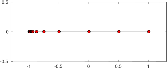
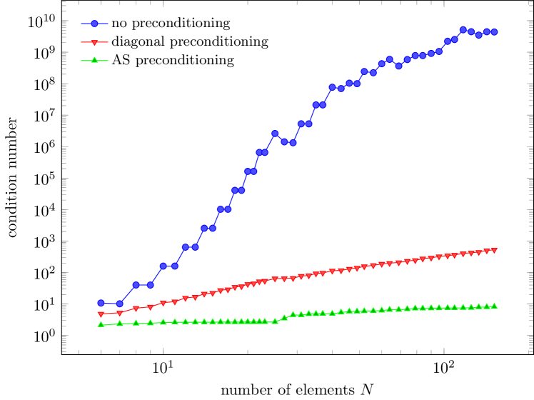
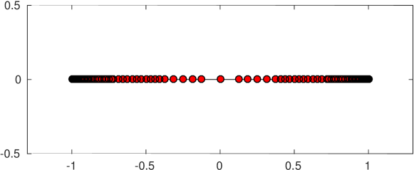
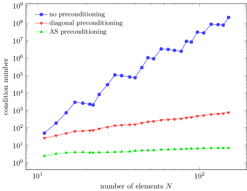
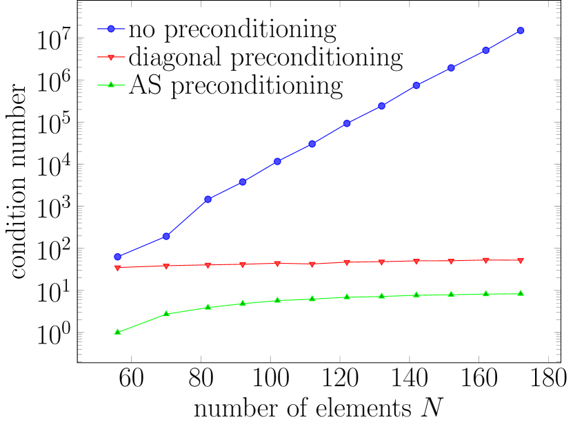
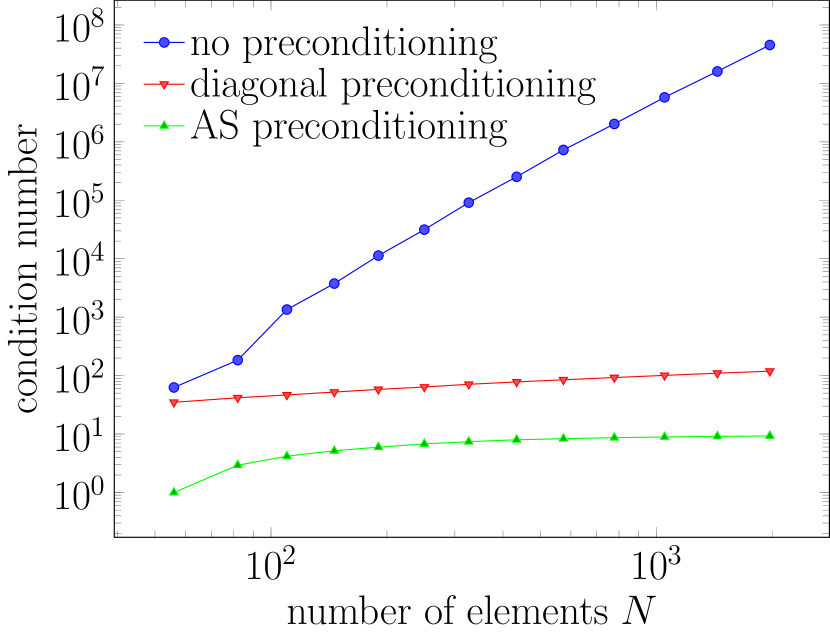
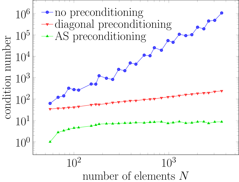
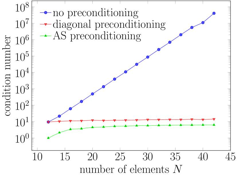
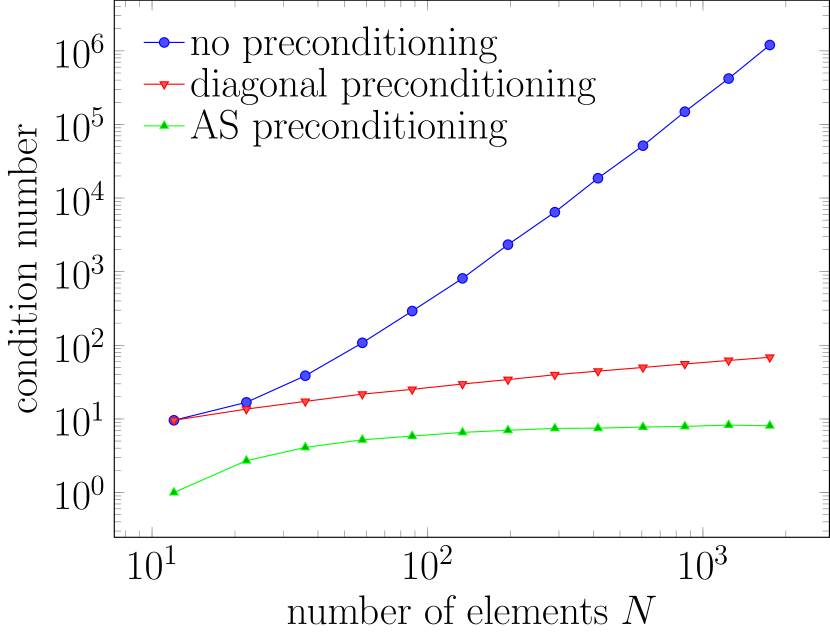
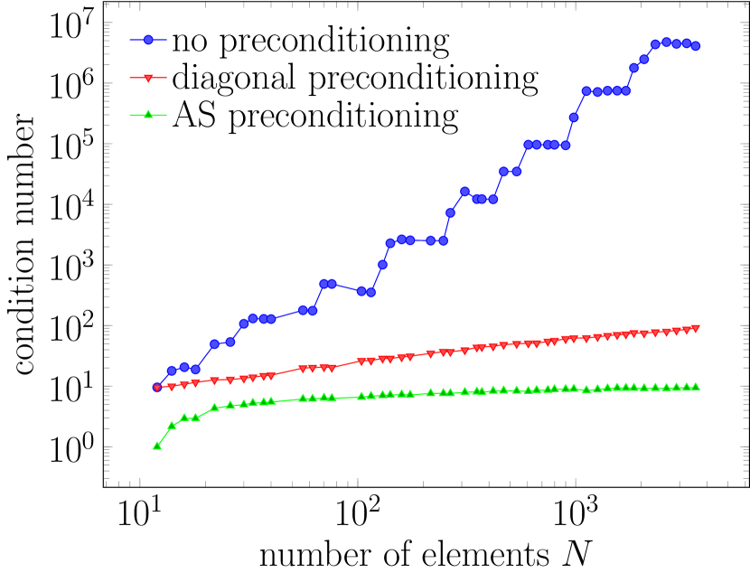
Figure 2. Example 4.1: Condition numbers of the preconditioned and non-preconditioned Galerkin matrix for an artificial refinement towards the left end point (left) and for the matrices arising from Algorithm 3.2 (right).

Refer to caption Refer to caption Refer to caption Refer to caption

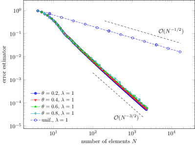
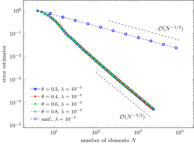
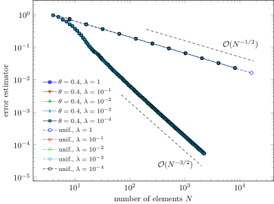
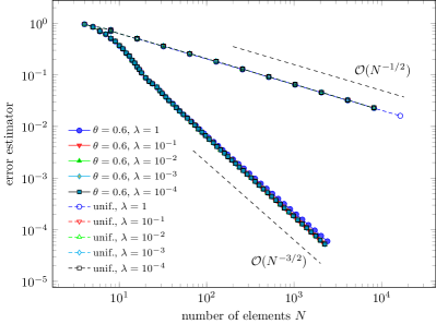
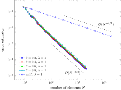
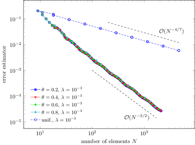
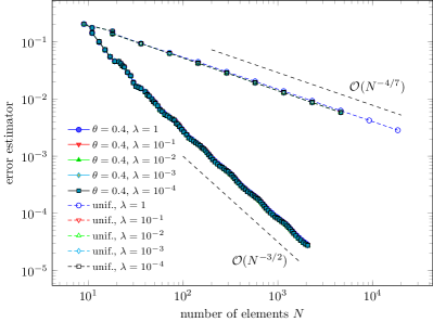
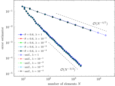
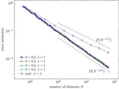
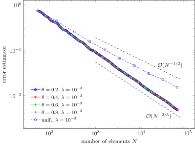
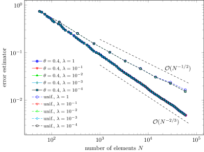
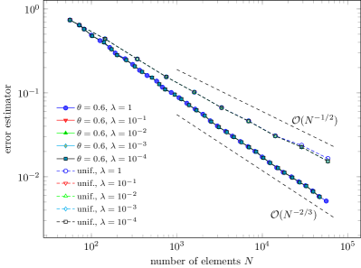
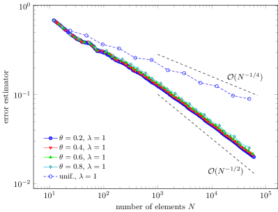
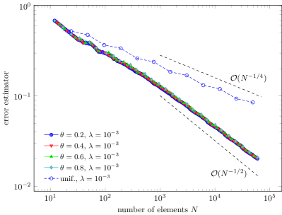
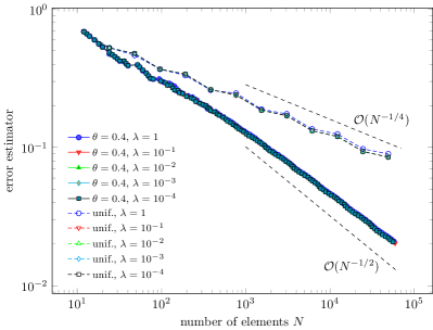
Figure 3. Example 4.1: Estimator convergence for fixed values of λ𝜆\lambda (left: λ=1𝜆1\lambda=1, right: λ=103𝜆superscript103\lambda=10^{-3}) and θ{0.2,0.4,0.6,0.8}𝜃0.20.40.60.8\theta\in\{0.2,0.4,0.6,0.8\} (top) and for fixed values of θ𝜃\theta (left: θ=0.4𝜃0.4\theta=0.4, right: θ=0.6𝜃0.6\theta=0.6) and λ{1,101,,104}𝜆1superscript101superscript104\lambda\in\{1,10^{-1},\ldots,10^{-4}\} (bottom).

Refer to caption Refer to caption

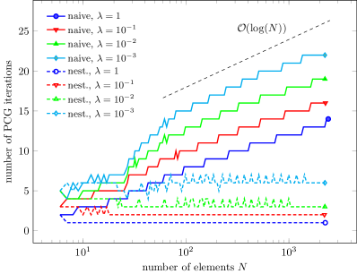
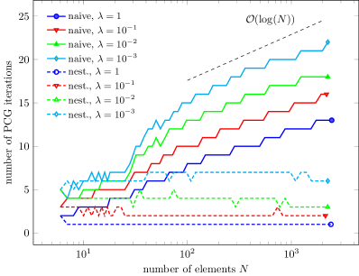
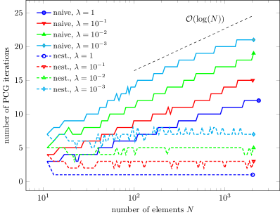
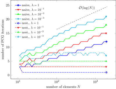
Figure 4. Example 4.1: Number of PCG iterations in Algorithm 3.2 for nested iteration (dashed lines), i.e., ϕ(j+1)0:=ϕjk¯assignsubscriptitalic-ϕ𝑗10subscriptitalic-ϕ𝑗¯𝑘\phi_{(j+1)0}:=\phi_{j\underline{k}} in Step (vi), and naive initial guess (solid lines), i.e., ϕ(j+1)0:=0assignsubscriptitalic-ϕ𝑗100\phi_{(j+1)0}:=0. We compare fixed values of θ𝜃\theta (left: θ=0.4𝜃0.4\theta=0.4, right: θ=0.6𝜃0.6\theta=0.6) and λ={1,101,,103}\lambda=\in\{1,10^{-1},\ldots,10^{-3}\}.

4.1. Slit Problem in 2D

Let Γ:=(1,1)×{0}assignΓ110\Gamma:=(-1,1)\times\{0\}, cf. Figure 2. We consider

(34) Vϕ=1 on Γ.𝑉italic-ϕ1 on Γ\displaystyle V\phi=1\quad\textrm{ on }\Gamma.

The unique exact solution of (34) reads ϕ(x,0):=2x/1x2assignsuperscriptitalic-ϕ𝑥02𝑥1superscript𝑥2\phi^{\star}(x,0):=-2x/\sqrt{1-x^{2}}. For uniform mesh-refinement, we thus expect a convergence order of 𝒪(N1/2)𝒪superscript𝑁12\mathcal{O}(N^{-1/2}), while the optimal rate is 𝒪(N3/2)𝒪superscript𝑁32\mathcal{O}(N^{-3/2}) with respect to the number of elements.

In Figure 3, we compare Algorithm 3.2 for different values for θ𝜃\theta and λ𝜆\lambda as well as uniform mesh-refinement. Uniform mesh-refinement leads only to the rate 𝒪(N1/2)𝒪superscript𝑁12\mathcal{O}(N^{-1/2}), while adaptivity, independently of the value of θ𝜃\theta and λ𝜆\lambda, regains the optimal rate 𝒪(N3/2)𝒪superscript𝑁32\mathcal{O}(N^{-3/2}). A naive initial guess in Step (vi) of Algorithm 3.2 (i.e., if ϕ(j+1)0:=0assignsubscriptitalic-ϕ𝑗100\phi_{(j+1)0}:=0) leads to a logarithmical growth of the number of PCG iterations, whereas for nested iteration ϕ(j+1)0:=ϕjk¯assignsubscriptitalic-ϕ𝑗10subscriptitalic-ϕ𝑗¯𝑘\phi_{(j+1)0}:=\phi_{j\underline{k}} (as formulated in Algorithm 3.2) the number of PCG iterations stays uniformly bounded, cf. Figure 4. Finally, Figure 2 shows the condition numbers for an artificial refinement towards the left end point and for Algorithm 3.2 with λ=103𝜆superscript103\lambda=10^{-3} and θ=0.5𝜃0.5\theta=0.5.

Refer to caption Refer to caption Refer to caption Refer to caption

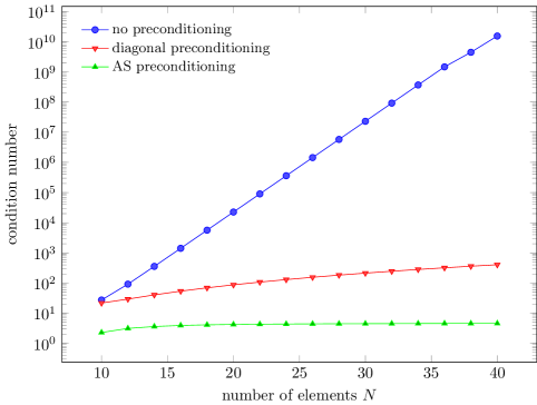
Figure 5. Example 4.2: Condition numbers of the preconditioned and non-preconditioned Galerkin matrix for an artificial refinement towards the reentrant corner (top) and for Algorithm 3.2 (bottom).

Refer to caption Refer to caption Refer to caption Refer to caption

Figure 6. Example 4.2: Estimator convergence for fixed values of λ𝜆\lambda (left: λ=1𝜆1\lambda=1, right: λ=103𝜆superscript103\lambda=10^{-3}) and θ{0.2,0.4,0.6,0.8}𝜃0.20.40.60.8\theta\in\{0.2,0.4,0.6,0.8\} (top) and for fixed values of θ𝜃\theta (left: θ=0.4𝜃0.4\theta=0.4, right: θ=0.6𝜃0.6\theta=0.6) and λ{1,101,,104}𝜆1superscript101superscript104\lambda\in\{1,10^{-1},\ldots,10^{-4}\} (bottom).

Refer to caption Refer to caption

Figure 7. Example 4.2: Number of PCG iterations in Algorithm 3.2 for nested iteration (dashed lines), i.e., ϕ(j+1)0:=ϕjk¯assignsubscriptitalic-ϕ𝑗10subscriptitalic-ϕ𝑗¯𝑘\phi_{(j+1)0}:=\phi_{j\underline{k}} in Step (vi), and naive initial guess (solid lines), i.e., ϕ(j+1)0:=0assignsubscriptitalic-ϕ𝑗100\phi_{(j+1)0}:=0. We compare fixed values of θ𝜃\theta (left: θ=0.4𝜃0.4\theta=0.4, right: θ=0.6𝜃0.6\theta=0.6) and λ={1,101,,103}\lambda=\in\{1,10^{-1},\ldots,10^{-3}\}.

4.2. Z-shaped domain in 2D

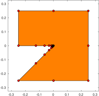
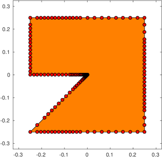
Let Γ:=ΩassignΓΩ\Gamma:=\partial\Omega be the boundary of the Z-shaped domain with reentrant corner at the origin (0,0)00(0,0), cf. Figure 5. The right-hand side is given by f=(K+1/2)g𝑓𝐾12𝑔f=(K+1/2)g with the double-layer operator K:H1/2(Γ)H1/2(Γ):𝐾superscript𝐻12Γsuperscript𝐻12ΓK\colon H^{1/2}(\Gamma)\to H^{1/2}(\Gamma). We note that the weakly-singular integral equation (1) is then equivalent to the Dirichlet problem

(35) Δu=0 in Ωsubject tou=g on Γ.formulae-sequenceΔ𝑢0 in Ωsubject to𝑢𝑔 on Γ\displaystyle\begin{split}-\Delta u&=0\quad\textrm{ in }\Omega\qquad\text{subject to}\qquad u=g\quad\textrm{ on }\Gamma.\end{split}

We prescribe the exact solution in 2D polar coordinates as

(36) u(x)=r4/7cos(4ξ/7)with x=r(cosξ,sinξ).formulae-sequence𝑢𝑥superscript𝑟474𝜉7with 𝑥𝑟𝜉𝜉\displaystyle u(x)=r^{4/7}\cos(4\,\xi/7)\quad\text{with }x=r(\cos\xi,\sin\xi).

Then, u𝑢u admits a generic singularity at the reentrant corner. The exact solution ϕsuperscriptitalic-ϕ\phi^{\star} of (1) is just the normal derivative of the solution u𝑢u.

We expect a convergence order of 𝒪(N4/7)𝒪superscript𝑁47\mathcal{O}(N^{-4/7}) for uniform mesh-refinement, and the optimal rate 𝒪(N3/2)𝒪superscript𝑁32\mathcal{O}(N^{-3/2}) for the adaptive strategy, which is seen in Figure 6 for different values of θ𝜃\theta and λ𝜆\lambda. A naive initial guess in Step (vi) of Algorithm 3.2 (i.e., if ϕ(j+1)0:=0assignsubscriptitalic-ϕ𝑗100\phi_{(j+1)0}:=0) leads to a logarithmical growth of the number of PCG iterations, whereas for nested iteration ϕ(j+1)0:=ϕjk¯assignsubscriptitalic-ϕ𝑗10subscriptitalic-ϕ𝑗¯𝑘\phi_{(j+1)0}:=\phi_{j\underline{k}} the number of PCG iterations stays uniformly bounded, cf. Figure 7. Figure 5 shows the condition numbers for an artificial refinement towards the reentrant corner as well as the condition numbers for Algorithm 3.2 with λ=103𝜆superscript103\lambda=10^{-3} and θ=0.5𝜃0.5\theta=0.5.

Refer to caption

Refer to caption

Refer to caption

Figure 8. Example 4.3: Condition numbers of the preconditioned and non-preconditioned Galerkin matrix for an artificial refinement towards one reentrant corner (left) or edge (middle), and for Algorithm 3.2 (right).

Refer to caption Refer to caption Refer to caption Refer to caption

Figure 9. Example 4.3: Estimator convergence for fixed values of λ𝜆\lambda (left: λ=1𝜆1\lambda=1, right: λ=103𝜆superscript103\lambda=10^{-3}) and θ{0.2,0.4,0.6,0.8}𝜃0.20.40.60.8\theta\in\{0.2,0.4,0.6,0.8\} (top) and for fixed values of θ𝜃\theta (left: θ=0.4𝜃0.4\theta=0.4, right: θ=0.6𝜃0.6\theta=0.6) and λ{1,101,,104}𝜆1superscript101superscript104\lambda\in\{1,10^{-1},\ldots,10^{-4}\} (bottom).

4.3. L-shaped domain in 3D

Let Γ:=ΩassignΓΩ\Gamma:=\partial\Omega be the boundary of the L-shaped domain Ω=(1,1)3\([1,0]×[0,1]×[1,1])Ω\superscript113100111\Omega=(-1,1)^{3}\backslash([-1,0]\times[0,1]\times[-1,1]), cf. Figure 8. The right-hand side is given by f=(K+1/2)g𝑓𝐾12𝑔f=(K+1/2)g with the double-layer operator K:H1/2(Γ)H1/2(Γ):𝐾superscript𝐻12Γsuperscript𝐻12ΓK\colon H^{1/2}(\Gamma)\to H^{1/2}(\Gamma). Again, the weakly-singular integral equation (1) is then equivalent to the Dirichlet problem (35). We prescribe the exact solution in 3D cylindrical coordinates as

(37) u(x)=zr2/3cos(2/3(ξπ/4))with x=(rcosξ,rsinξ,z).formulae-sequence𝑢𝑥𝑧superscript𝑟2323𝜉𝜋4with 𝑥𝑟𝜉𝑟𝜉𝑧\displaystyle u(x)=z\,r^{2/3}\cos(2/3\,(\xi-\pi/4))\quad\text{with }x=(r\cos\xi,r\sin\xi,z).

Note that u𝑢u admits a singularity along the reentrant edge. The exact solution ϕsuperscriptitalic-ϕ\phi^{\star} of (1) is just the normal derivative of the exact solution u𝑢u.

In Figure 9, we compare Algorithm 3.2 with different values for θ𝜃\theta and λ𝜆\lambda to uniform mesh-refinement. Uniform mesh-refinement leads only to a reduced rate of 𝒪(N1/2)𝒪superscript𝑁12\mathcal{O}(N^{-1/2}), while adaptivity, independently of θ𝜃\theta and λ𝜆\lambda, leads to the improved rate of approximately 𝒪(N2/3)𝒪superscript𝑁23\mathcal{O}(N^{-2/3}). While one would expect 𝒪(N3/4)𝒪superscript𝑁34\mathcal{O}(N^{-3/4}) for smooth exact solutions ϕsuperscriptitalic-ϕ\phi^{\star}, this would require anisotropic elements along the reentrant edge for the present solution ϕ=nusuperscriptitalic-ϕsubscript𝑛𝑢\phi^{\star}=\partial_{n}u. Since NVB guarantees uniform γ𝛾\gamma-shape regularity of the meshes, the latter is not possible and hence leads to a reduced optimal rate. Finally, Figure 8 shows the condition numbers for (diagonal or additive Schwarz) preconditioning and no preconditioning for artificial refinements towards one reentrant corner or the reentrant edge as well as the condition numbers of the matrices arising from Algorithm 3.2 with λ=103𝜆superscript103\lambda=10^{-3} and θ=0.5𝜃0.5\theta=0.5.

Refer to caption

Refer to caption

Refer to caption

Figure 10. Example 4.4: Condition numbers of the preconditioned and non-preconditioned Galerkin matrix for an artificial refinement towards the right corner (left), the right edges (middle), and for Algorithm 3.2 (right).

Refer to caption Refer to caption Refer to caption Refer to caption

Figure 11. Example 4.4: Estimator convergence for fixed values of λ𝜆\lambda (left: λ=1𝜆1\lambda=1, right: λ=103𝜆superscript103\lambda=10^{-3}) and θ{0.2,0.4,0.6,0.8}𝜃0.20.40.60.8\theta\in\{0.2,0.4,0.6,0.8\} (top) and for fixed values of θ𝜃\theta (left: θ=0.4𝜃0.4\theta=0.4, right: θ=0.6𝜃0.6\theta=0.6) and λ{1,101,,104}𝜆1superscript101superscript104\lambda\in\{1,10^{-1},\ldots,10^{-4}\} (bottom).

4.4. Screen problem in 3D

Let Γ:=((1,1)2[0,1])×{0}assignΓsuperscript112010\Gamma:=((-1,1)^{2}\setminus[0,1])\times\{0\}, rotated by 3π/43𝜋43\pi/4, cf. Figure 10. We consider the weakly-singular integral equation Vϕ=1𝑉superscriptitalic-ϕ1V\phi^{\star}=1 on ΓΓ\Gamma. The exact solution ϕH~1/2(Γ)superscriptitalic-ϕsuperscript~𝐻12Γ\phi^{\star}\in\widetilde{H}^{-1/2}(\Gamma) is unknown.

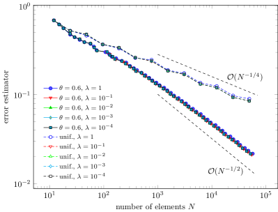
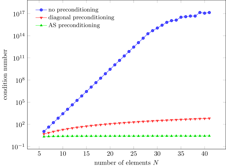
For the numerical solution of the Galerkin system, we employ PCG with the additive Schwarz preconditioner from Section 3.1. We note that Theorem 3.1 does not cover this setting. In particular, we note that the proposed additive Schwarz preconditioner from Section 3.1 appears to be optimal, while the mathematical optimality proof still remains open for screens, cf. Figure 10.

In Figure 11, we compare Algorithm 3.2 with different values for θ𝜃\theta and λ𝜆\lambda to uniform mesh-refinement. We see that uniform mesh-refinement leads only to a reduced rate of 𝒪(N1/4)𝒪superscript𝑁14\mathcal{O}(N^{-1/4}), while adaptivity, independently of θ𝜃\theta and λ𝜆\lambda, leads to the improved rate of approximately 𝒪(N1/2)𝒪superscript𝑁12\mathcal{O}(N^{-1/2}).

Refer to caption Refer to caption Refer to caption Refer to caption

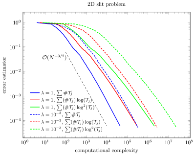
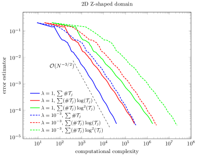
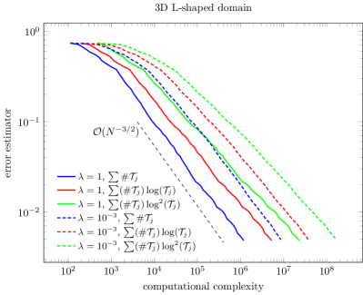
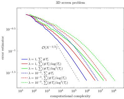
Figure 12. To underline the quasi-optimal computational complexity of Algorithm 3.2, we plot the error estimator ηj(ϕjk¯)subscript𝜂𝑗subscriptitalic-ϕ𝑗¯𝑘\eta_{j}(\phi_{j\underline{k}}) in the different experiments over the cumulative quantities (j,k)(j,k)#𝒯jsubscript𝑗𝑘superscript𝑗superscript𝑘#subscript𝒯𝑗\sum_{(j,k)\leq(j^{\prime},k^{\prime})}\#\mathcal{T}_{j}, (j,k)(j,k)(#𝒯j)log(#𝒯j)subscript𝑗𝑘superscript𝑗superscript𝑘#subscript𝒯𝑗#subscript𝒯𝑗\sum_{(j,k)\leq(j^{\prime},k^{\prime})}(\#\mathcal{T}_{j})\log(\#\mathcal{T}_{j}) and (j,k)(j,k)(#𝒯j)log2(#𝒯j)subscript𝑗𝑘superscript𝑗superscript𝑘#subscript𝒯𝑗superscript2#subscript𝒯𝑗\sum_{(j,k)\leq(j^{\prime},k^{\prime})}(\#\mathcal{T}_{j})\log^{2}(\#\mathcal{T}_{j}) for θ=0.4𝜃0.4\theta=0.4 and λ{1,103}𝜆1superscript103\lambda\in\{1,10^{-3}\}.

4.5. Computational complexity

With Figure 12, we aim to underpin the almost optimal computational complexity of Algorithm 3.2 (see Corollary 3.3). To this end, we plot the error estimator ηj(ϕjk)subscript𝜂𝑗subscriptitalic-ϕ𝑗𝑘\eta_{j}(\phi_{jk}) over the cumulative sums

(j,k)(j,k)cost(𝒯j)withcost(𝒯j){#𝒯j,(#𝒯j)log(#𝒯j),(#𝒯j)log2(#𝒯j)}subscript𝑗𝑘superscript𝑗superscript𝑘costsubscript𝒯jwithcostsubscript𝒯j#subscript𝒯j#subscript𝒯j#subscript𝒯j#subscript𝒯jsuperscript2#subscript𝒯j\displaystyle\sum_{(j,k)\leq(j^{\prime},k^{\prime})}\rm cost(\mathcal{T}_{j})\quad\text{with}\quad\rm cost(\mathcal{T}_{j})\in\big{\{}\#\mathcal{T}_{j}\,,\,(\#\mathcal{T}_{j})\,\log(\#\mathcal{T}_{j})\,,\,(\#\mathcal{T}_{j})\,\log^{2}(\#\mathcal{T}_{j})\big{\}}

for θ=0.4𝜃0.4\theta=0.4 and λ{1,103}𝜆1superscript103\lambda\in\{1,10^{-3}\}. The negative impact of the logarithmic terms on the (preasymptotic) convergence rate is clearly visible.

5. Proof of Theorem 3.1 (Optimal Multilevel Preconditioner)

For d=2𝑑2d=2, we refer to [FFPS17b, Füh14] and thus focus only on d=3𝑑3d=3 and Γ=ΩΓΩ\Gamma=\partial\Omega. Due to our additional assumption, 𝒯0=𝒯^0|Γsubscript𝒯0evaluated-atsubscript^𝒯0Γ\mathcal{T}_{0}=\widehat{\mathcal{T}}_{0}|_{\Gamma} is the restriction of a conforming simplicial triangulation 𝒯^0subscript^𝒯0\widehat{\mathcal{T}}_{0} of ΩΩ\Omega to the boundary ΓΓ\Gamma. Moreover, 2D NVB refinement of 𝒯0subscript𝒯0\mathcal{T}_{0} (on the boundary ΓΓ\Gamma) is a special case of 3D NVB refinement of 𝒯^0subscript^𝒯0\widehat{\mathcal{T}}_{0} (in the volume ΩΩ\Omega) plus restriction to the boundary; see, e.g., [Ste08]. Hence, each mesh 𝒯𝕋=refine(𝒯0)subscript𝒯𝕋refinesubscript𝒯0\mathcal{T}_{\bullet}\in\mathbb{T}={\rm refine}(\mathcal{T}_{0}) is the restriction of a conforming NVB refinement 𝒯^𝕋^:=refine(𝒯^0)subscript^𝒯^𝕋assignrefinesubscript^𝒯0\widehat{\mathcal{T}}_{\bullet}\in\widehat{\mathbb{T}}:={\rm refine}(\widehat{\mathcal{T}}_{0}), i.e., 𝒯=𝒯^|Γsubscript𝒯evaluated-atsubscript^𝒯Γ\mathcal{T}_{\bullet}=\widehat{\mathcal{T}}_{\bullet}|_{\Gamma}. Throughout, let 𝒯^𝕋^subscript^𝒯^𝕋\widehat{\mathcal{T}}_{\bullet}\in\widehat{\mathbb{T}} be the coarsest extension of 𝒯𝕋subscript𝒯𝕋\mathcal{T}_{\bullet}\in\mathbb{T}. Recall that NVB is a binary refinement rule. Therefore, 𝒯refine(𝒯)subscript𝒯refinesubscript𝒯\mathcal{T}_{\circ}\in{\rm refine}(\mathcal{T}_{\bullet}) also implies that 𝒯^refine(𝒯^)subscript^𝒯refinesubscript^𝒯\widehat{\mathcal{T}}_{\circ}\in{\rm refine}(\widehat{\mathcal{T}}_{\bullet}). Finally, we note that all triangulations 𝒯^𝕋^subscript^𝒯^𝕋\widehat{\mathcal{T}}_{\bullet}\in\widehat{\mathbb{T}} are uniformly γ𝛾\gamma-shape regular, i.e.,

maxT^𝒯^diam(T^)|T^|1/3γ<.subscript^𝑇subscript^𝒯diam^𝑇superscript^𝑇13𝛾\displaystyle\max_{\widehat{T}\in\widehat{\mathcal{T}}_{\bullet}}\frac{{\rm diam}(\widehat{T})}{|\widehat{T}|^{1/3}}\leq\gamma<\infty.

where γ𝛾\gamma depends only on 𝒯^0subscript^𝒯0\widehat{\mathcal{T}}_{0}.

Our argument adapts ideas from [HM12], where a subspace decomposition for the lowest-order Nédélec space 𝓝𝓓1(𝒯^)𝓝superscript𝓓1subscript^𝒯\boldsymbol{\mathcal{N}}\!\boldsymbol{\mathcal{D}}^{1}(\widehat{\mathcal{T}}_{\bullet}) (see, e.g., [HZ09]) in 𝑯(𝐜𝐮𝐫𝐥;Ω)𝑯𝐜𝐮𝐫𝐥Ω\boldsymbol{H}(\boldsymbol{\operatorname{curl}}\,;\,\Omega) implies a decomposition of the corresponding discrete trace space. While the original idea dates back to [Osw99], a nice summary of the argument is found in [HM12, Section 2].

   Remark 11. (i) Our proof is based on the construction of an extension operator from 𝒫0(𝒯)superscriptsubscript𝒫0subscript𝒯\mathcal{P}_{*}^{0}(\mathcal{T}_{\bullet}) to 𝓝𝓓1(𝒯^)𝓝superscript𝓓1subscript^𝒯\boldsymbol{\mathcal{N}}\!\boldsymbol{\mathcal{D}}^{1}(\widehat{\mathcal{T}}_{\bullet}), see Lemma 5.1 below. It is not clear if such an operator can be constructed for the case ΓΩΓΩ\Gamma\subsetneqq\partial\Omega.

(ii) In [HJHM15], a subspace decomposition of the lowest-order Raviart–Thomas space 𝓡𝓣0(𝒯^)𝓡superscript𝓣0subscript^𝒯\boldsymbol{\mathcal{R}}\!\boldsymbol{\mathcal{T}}^{0}(\widehat{\mathcal{T}}_{\bullet}) (see, e.g., [XCN09]) in 𝐇(𝐝𝐢𝐯;Ω)𝐇𝐝𝐢𝐯Ω\boldsymbol{H}(\boldsymbol{\operatorname{div}}\,;\,\Omega) implies a decomposition of the corresponding normal trace space 𝒫0(𝒯)superscript𝒫0subscript𝒯\mathcal{P}^{0}(\mathcal{T}_{\bullet}). Due to different scaling properties of the Raviart–Thomas basis functions (in the 𝐇(𝐝𝐢𝐯;Ω)𝐇𝐝𝐢𝐯Ω\boldsymbol{H}(\boldsymbol{\operatorname{div}}\,;\,\Omega) norm) and their normal trace (in the H1/2(Γ)superscript𝐻12ΓH^{-1/2}(\Gamma) norm), this argument does not apply in our case.    

5.1. Discrete spaces and extensions

Let ^^absentsubscript\widehat{}\mathcal{E}_{\bullet} (resp. 𝒩^subscript^𝒩\widehat{\mathcal{N}}_{\bullet}) denote the set of all edges (resp. all nodes) of 𝒯^𝕋^subscript^𝒯^𝕋\widehat{\mathcal{T}}_{\bullet}\in\widehat{\mathbb{T}}. For each node 𝒙𝒩^𝒙subscript^𝒩\boldsymbol{x}\in\widehat{\mathcal{N}}_{\bullet}, let η,𝒙𝒮1(𝒯^)subscript𝜂𝒙superscript𝒮1subscript^𝒯\eta_{\bullet,\boldsymbol{x}}\in\mathcal{S}^{1}(\widehat{\mathcal{T}}_{\bullet}) be the corresponding hat function, i.e., η,𝒙subscript𝜂𝒙\eta_{\bullet,\boldsymbol{x}} is 𝒯^subscript^𝒯\widehat{\mathcal{T}}_{\bullet}-piecewise affine and globally continuous with η,𝒙(𝒚)=δ𝒙𝒚subscript𝜂𝒙𝒚subscript𝛿𝒙𝒚\eta_{\bullet,\boldsymbol{x}}(\boldsymbol{y})=\delta_{\boldsymbol{x}\boldsymbol{y}} for all 𝒙,𝒚𝒩^𝒙𝒚subscript^𝒩\boldsymbol{x},\boldsymbol{y}\in\widehat{\mathcal{N}}_{\bullet}. For E^𝐸^absentsubscriptE\in\widehat{}\mathcal{E}_{\bullet}, let 𝒖,E𝓝𝓓1(𝒯^)subscript𝒖𝐸𝓝superscript𝓓1subscript^𝒯{\boldsymbol{u}}_{\bullet,E}\in\boldsymbol{\mathcal{N}}\!\boldsymbol{\mathcal{D}}^{1}(\widehat{\mathcal{T}}_{\bullet}) denote the corresponding Nédélec basis function, i.e., for K𝒯^𝐾subscript^𝒯K\in\widehat{\mathcal{T}}_{\bullet} with E=conv{𝒙,𝒚}K𝐸conv𝒙𝒚𝐾E={\rm conv}\{\boldsymbol{x},\boldsymbol{y}\}\subset\partial K, it holds that

(38) 𝒖,E|K=C(η,𝒙η,𝒚η,𝒚η,𝒙),evaluated-atsubscript𝒖𝐸𝐾𝐶subscript𝜂𝒙subscript𝜂𝒚subscript𝜂𝒚subscript𝜂𝒙\displaystyle{\boldsymbol{u}}_{\bullet,E}|_{K}=C(\eta_{\bullet,\boldsymbol{x}}\nabla\eta_{\bullet,\boldsymbol{y}}-\eta_{\bullet,\boldsymbol{y}}\nabla\eta_{\bullet,\boldsymbol{x}}),

where C>0𝐶0C>0 is chosen such that E𝒖,E𝑑s=|E|δEEsubscriptsuperscript𝐸subscript𝒖𝐸differential-d𝑠𝐸subscript𝛿𝐸superscript𝐸\int_{E^{\prime}}{\boldsymbol{u}}_{\bullet,E}\,ds=|E|\,\delta_{EE^{\prime}} for all E,E^𝐸superscript𝐸^absentsubscriptE,E^{\prime}\in\widehat{}\mathcal{E}_{\bullet}. Scaling arguments yield the next lemma. The proof follows the lines of [HM12, Lemma 5.7].

   Lemma 12.  For E𝐸subscriptE\in\mathcal{E}_{\bullet}, recall the Haar function φ,E𝒫0(𝒯)subscript𝜑𝐸superscript𝒫0subscript𝒯\varphi_{\bullet,E}\in\mathcal{P}^{0}(\mathcal{T}_{\bullet}) from (21). Let 𝐮,E𝓝𝓓1(𝒯^)subscript𝐮𝐸𝓝superscript𝓓1subscript^𝒯{\boldsymbol{u}}_{\bullet,E}\in\boldsymbol{\mathcal{N}}\!\boldsymbol{\mathcal{D}}^{1}(\widehat{\mathcal{T}}_{\bullet}) denote the corresponding Nédélec basis function; see (38). Then,

(39) φ,E=𝐜𝐮𝐫𝐥𝒖,E𝒏|Γ and φ,EH1/2(Γ)𝒖,E𝑯(𝐜𝐮𝐫𝐥;Ω)Cφ,EH1/2(Γ),subscript𝜑𝐸evaluated-at𝐜𝐮𝐫𝐥subscript𝒖𝐸𝒏Γ and subscriptnormsubscript𝜑𝐸superscript𝐻12Γsubscriptnormsubscript𝒖𝐸𝑯𝐜𝐮𝐫𝐥Ω𝐶subscriptnormsubscript𝜑𝐸superscript𝐻12Γ\displaystyle\varphi_{\bullet,E}=\boldsymbol{\operatorname{curl}}\,{\boldsymbol{u}}_{\bullet,E}\cdot{\boldsymbol{n}}|_{\Gamma}\,\text{ and }\,\,\|\varphi_{\bullet,E}\|_{H^{-1/2}(\Gamma)}\leq\|{\boldsymbol{u}}_{\bullet,E}\|_{\boldsymbol{H}(\boldsymbol{\operatorname{curl}}\,;\,\Omega)}\leq C\,\|\varphi_{\bullet,E}\|_{H^{-1/2}(\Gamma)},

where C>0𝐶0C>0 depends only on ΩΩ\Omega and the γ𝛾\gamma-shape regularity of 𝒯^subscript^𝒯\widehat{\mathcal{T}}_{\bullet}. ∎   

The following lemma holds for (simply) connected Lipschitz domains ΩΩ\Omega and follows essentially from [AGS16]. Recall 𝒫0(𝒯)subscriptsuperscript𝒫0subscript𝒯\mathcal{P}^{0}_{*}(\mathcal{T}_{\bullet}) from (22).

   Lemma 13.  There exists a linear operator 𝐄:𝒫0(𝒯)𝓝𝓓1(𝒯^):subscript𝐄superscriptsubscript𝒫0subscript𝒯𝓝superscript𝓓1subscript^𝒯\boldsymbol{E}_{\bullet}:\mathcal{P}_{*}^{0}(\mathcal{T}_{\bullet})\to\boldsymbol{\mathcal{N}}\!\boldsymbol{\mathcal{D}}^{1}(\widehat{\mathcal{T}}_{\bullet}) such that

(40) 𝐜𝐮𝐫𝐥(𝑬ψ)𝒏|Γ=ψ and 𝑬ψ𝑯(𝐜𝐮𝐫𝐥;Ω)CψH1/2(Γ) for all ψ𝒫0(𝒯).evaluated-at𝐜𝐮𝐫𝐥subscript𝑬subscript𝜓𝒏Γsubscript𝜓 and subscriptnormsubscript𝑬subscript𝜓𝑯𝐜𝐮𝐫𝐥Ω𝐶subscriptnormsubscript𝜓superscript𝐻12Γ for all subscript𝜓superscriptsubscript𝒫0subscript𝒯\displaystyle\boldsymbol{\operatorname{curl}}\,(\boldsymbol{E}_{\bullet}\psi_{\bullet})\cdot{\boldsymbol{n}}|_{\Gamma}=\psi_{\bullet}\text{ and }\|\boldsymbol{E}_{\bullet}\psi_{\bullet}\|_{\boldsymbol{H}(\boldsymbol{\operatorname{curl}}\,;\,\Omega)}\leq C\,\|\psi_{\bullet}\|_{H^{-1/2}(\Gamma)}\text{ for all }\psi_{\bullet}\in\mathcal{P}_{*}^{0}(\mathcal{T}_{\bullet}).

The constant C>0𝐶0C>0 depends only on γ𝛾\gamma-shape regularity of 𝒯^subscript^𝒯\widehat{\mathcal{T}}_{\bullet}.    

Proof.

Let ψ𝒫0(𝒯)subscript𝜓superscriptsubscript𝒫0subscript𝒯\psi_{\bullet}\in\mathcal{P}_{*}^{0}(\mathcal{T}_{\bullet}). First, [AGS16, Theorem 2.1] provides 𝝈𝓡𝓣0(𝒯^)subscript𝝈𝓡superscript𝓣0subscript^𝒯{\boldsymbol{\sigma}}_{\bullet}\in\boldsymbol{\mathcal{R}}\!\boldsymbol{\mathcal{T}}^{0}(\widehat{\mathcal{T}}_{\bullet}) with

𝝈𝒏|Γ=ψ,𝐝𝐢𝐯𝝈=0,and𝝈𝑯(𝐝𝐢𝐯;Ω)ψH1/2(Ω).formulae-sequenceevaluated-atsubscript𝝈𝒏Γsubscript𝜓formulae-sequence𝐝𝐢𝐯subscript𝝈0andless-than-or-similar-tosubscriptnormsubscript𝝈𝑯𝐝𝐢𝐯Ωsubscriptnormsubscript𝜓superscript𝐻12Ω\displaystyle{\boldsymbol{\sigma}}_{\bullet}\cdot{\boldsymbol{n}}|_{\Gamma}=\psi_{\bullet},\quad\boldsymbol{\operatorname{div}}\,{\boldsymbol{\sigma}}_{\bullet}=0,\quad\text{and}\quad\|{\boldsymbol{\sigma}}_{\bullet}\|_{\boldsymbol{H}(\boldsymbol{\operatorname{div}}\,;\,\Omega)}\lesssim\|\psi_{\bullet}\|_{H^{-1/2}(\partial\Omega)}.

Then, [AGS16, Lemma 4.3] provides 𝑬ψ:=𝒗𝓝𝓓1(𝒯^)assignsubscript𝑬subscript𝜓subscript𝒗𝓝superscript𝓓1subscript^𝒯\boldsymbol{E}_{\bullet}\psi_{\bullet}:={\boldsymbol{v}}_{\bullet}\in\boldsymbol{\mathcal{N}}\!\boldsymbol{\mathcal{D}}^{1}(\widehat{\mathcal{T}}_{\bullet}) such that

𝐜𝐮𝐫𝐥𝒗=𝝈and𝒗𝑯(𝐜𝐮𝐫𝐥;Ω)𝝈𝑯(𝐝𝐢𝐯;Ω).formulae-sequence𝐜𝐮𝐫𝐥subscript𝒗subscript𝝈andless-than-or-similar-tosubscriptnormsubscript𝒗𝑯𝐜𝐮𝐫𝐥Ωsubscriptnormsubscript𝝈𝑯𝐝𝐢𝐯Ω\displaystyle\boldsymbol{\operatorname{curl}}\,{\boldsymbol{v}}_{\bullet}={\boldsymbol{\sigma}}_{\bullet}\quad\text{and}\quad\|{\boldsymbol{v}}_{\bullet}\|_{\boldsymbol{H}(\boldsymbol{\operatorname{curl}}\,;\,\Omega)}\lesssim\|{\boldsymbol{\sigma}}_{\bullet}\|_{\boldsymbol{H}(\boldsymbol{\operatorname{div}}\,;\,\Omega)}.

Combining these results, we conclude the proof. ∎

5.2. Abstract additive Schwarz preconditioners

Let 𝒳𝒳\mathcal{X} denote some finite dimensional Hilbert space with norm 𝒳\|\cdot\|_{\mathcal{X}} and subspace decomposition

𝒳=i𝒳i,𝒳subscript𝑖subscript𝒳𝑖\displaystyle\mathcal{X}=\sum_{i\in\mathcal{I}}\mathcal{X}_{i},

where \mathcal{I} is a finite index set. The additive Schwarz operator is given by 𝒮=i𝒮i𝒮subscript𝑖subscript𝒮𝑖\mathcal{S}=\sum_{i\in\mathcal{I}}\mathcal{S}_{i}, where 𝒮isubscript𝒮𝑖\mathcal{S}_{i} is the 𝒳𝒳\mathcal{X}-orthogonal projection onto 𝒳isubscript𝒳𝑖\mathcal{X}_{i}, i.e.,

𝒮ix,xi𝒳=x,xi𝒳for all xi𝒳i and all x𝒳,formulae-sequencesubscriptsubscript𝒮𝑖𝑥subscript𝑥𝑖𝒳subscript𝑥subscript𝑥𝑖𝒳for all subscript𝑥𝑖subscript𝒳𝑖 and all 𝑥𝒳\displaystyle\langle\mathcal{S}_{i}x\,,\,x_{i}\rangle_{\mathcal{X}}=\langle x\,,\,x_{i}\rangle_{\mathcal{X}}\quad\text{for all }x_{i}\in\mathcal{X}_{i}\text{ and all }x\in\mathcal{X},

where ,𝒳subscript𝒳\langle\cdot\,,\,\cdot\rangle_{\mathcal{X}} denotes the scalar product on 𝒳𝒳\mathcal{X}. Then, the operator 𝒮𝒮\mathcal{S} is positive definite and symmetric (with respect to ,𝒳subscript𝒳\langle\cdot\,,\,\cdot\rangle_{\mathcal{X}}). Define the multilevel norm

(41) |x|𝒳2:=inf{ixi𝒳2:x=ixiwith xi𝒳i for all i}.assignsuperscriptsubscriptnorm𝑥𝒳2infimumconditional-setsubscript𝑖:evaluated-atsubscript𝑥𝑖𝒳2formulae-sequence𝑥subscript𝑖subscript𝑥𝑖with subscript𝑥𝑖subscript𝒳𝑖 for all 𝑖\displaystyle|\!|\!|\,x\,|\!|\!|_{\mathcal{X}}^{2}:=\inf\Big{\{}\sum_{i\in\mathcal{I}}\|x_{i}\|_{\mathcal{X}}^{2}\,:\,x=\sum_{i\in\mathcal{I}}x_{i}\quad\text{with }x_{i}\in\mathcal{X}_{i}\text{ for all }i\in\mathcal{I}\Big{\}}.

It is proved, e.g., in [Osw94, Theorem 16] that 𝒮1x,x𝒳=|x|𝒳2subscriptsuperscript𝒮1𝑥𝑥𝒳superscriptsubscriptnorm𝑥𝒳2\langle\mathcal{S}^{-1}x\,,\,x\rangle_{\mathcal{X}}=|\!|\!|\,x\,|\!|\!|_{\mathcal{X}}^{2}. Let C>0𝐶0C>0. If

C1x𝒳|x|𝒳Cx𝒳for all x𝒳,formulae-sequencesuperscript𝐶1subscriptnorm𝑥𝒳subscriptnorm𝑥𝒳𝐶subscriptnorm𝑥𝒳for all 𝑥𝒳\displaystyle C^{-1}\|x\|_{\mathcal{X}}\leq|\!|\!|\,x\,|\!|\!|_{\mathcal{X}}\leq C\,\|x\|_{\mathcal{X}}\quad\text{for all }x\in\mathcal{X},

then the extreme eigenvalues of 𝒮1superscript𝒮1\mathcal{S}^{-1} (and hence those of 𝒮𝒮\mathcal{S}) are bounded (from above and below). In particular, the additive Schwarz operator 𝒮𝒮\mathcal{S} is optimal in the sense that its condition number (ratio of largest and smallest eigenvalues) depends only on C>0𝐶0C>0.

Let 𝑺𝑺\boldsymbol{S} denote the matrix representation of 𝒮𝒮\mathcal{S}. Then, the norm equivalence from above and the latter observations imply that the condition number of 𝑺𝑺\boldsymbol{S} is bounded. The abstract theory on additive Schwarz operators given in [TW05, Chapter 2] shows that 𝑺𝑺\boldsymbol{S} has the form 𝑺=𝑷1𝑨𝑺superscript𝑷1𝑨\boldsymbol{S}=\boldsymbol{P}^{-1}\boldsymbol{A}, where 𝑨𝑨\boldsymbol{A} is the Galerkin matrix of ,𝒳subscript𝒳\langle\cdot\,,\,\cdot\rangle_{\mathcal{X}}. Therefore, boundedness of the condition number of 𝑺𝑺\boldsymbol{S} implies optimality of the preconditioner 𝑷1superscript𝑷1\boldsymbol{P}^{-1}.

We shortly discuss the matrix representation (24) of the additive Schwarz preconditioner 𝑷1superscript𝑷1\boldsymbol{P}^{-1}. Following [TW05, Chapter 2], let 𝑨isubscript𝑨𝑖\boldsymbol{A}_{i} denote the Galerkin matrix of ,𝒳subscript𝒳\langle\cdot\,,\,\cdot\rangle_{\mathcal{X}} restricted to 𝒳isubscript𝒳𝑖\mathcal{X}_{i}, and let 𝑰isubscript𝑰𝑖\boldsymbol{I}_{i} denote the matrix that realizes the embedding from 𝒳i𝒳subscript𝒳𝑖𝒳\mathcal{X}_{i}\to\mathcal{X}. We consider the matrix representation of 𝒮i:𝒳𝒳i𝒳:subscript𝒮𝑖𝒳subscript𝒳𝑖𝒳\mathcal{S}_{i}:\mathcal{X}\to\mathcal{X}_{i}\subset\mathcal{X}. Let x𝒳𝑥𝒳x\in\mathcal{X} with coordinate vector 𝒙𝒙\boldsymbol{x}, and let xi𝒳isubscript𝑥𝑖subscript𝒳𝑖x_{i}\in\mathcal{X}_{i} be arbitrary with coordinate vector 𝒙isubscript𝒙𝑖\boldsymbol{x}_{i}. The defining relation

𝒮ix,xi𝒳=x,xi𝒳for all xi𝒳iformulae-sequencesubscriptsubscript𝒮𝑖𝑥subscript𝑥𝑖𝒳subscript𝑥subscript𝑥𝑖𝒳for all subscript𝑥𝑖subscript𝒳𝑖\displaystyle\langle\mathcal{S}_{i}x\,,\,x_{i}\rangle_{\mathcal{X}}=\langle x\,,\,x_{i}\rangle_{\mathcal{X}}\quad\text{for all }x_{i}\in\mathcal{X}_{i}

of 𝒮isubscript𝒮𝑖\mathcal{S}_{i} then reads in matrix-vector form (with 𝑺isubscript𝑺𝑖\boldsymbol{S}_{i} being the matrix representation of 𝒮isubscript𝒮𝑖\mathcal{S}_{i}) as

𝒙i(𝑨i𝑺i𝒙)=(𝑰i𝒙i)(𝑨𝒙)for all coefficient vectors 𝒙i,subscript𝒙𝑖subscript𝑨𝑖subscript𝑺𝑖𝒙subscript𝑰𝑖subscript𝒙𝑖𝑨𝒙for all coefficient vectors subscript𝒙𝑖\displaystyle\boldsymbol{x}_{i}\cdot(\boldsymbol{A}_{i}\boldsymbol{S}_{i}\boldsymbol{x})=(\boldsymbol{I}_{i}\boldsymbol{x}_{i})\cdot(\boldsymbol{A}\boldsymbol{x})\quad\text{for all coefficient vectors }\boldsymbol{x}_{i},

or equivalently

𝑨i𝑺i𝒙=𝑰iT𝑨𝒙.subscript𝑨𝑖subscript𝑺𝑖𝒙superscriptsubscript𝑰𝑖𝑇𝑨𝒙\displaystyle\boldsymbol{A}_{i}\boldsymbol{S}_{i}\boldsymbol{x}=\boldsymbol{I}_{i}^{T}\boldsymbol{A}\boldsymbol{x}.

Since 𝑨isubscript𝑨𝑖\boldsymbol{A}_{i} is invertible, we have that

𝑺i=𝑨i1𝑰iT𝑨.subscript𝑺𝑖superscriptsubscript𝑨𝑖1superscriptsubscript𝑰𝑖𝑇𝑨\displaystyle\boldsymbol{S}_{i}=\boldsymbol{A}_{i}^{-1}\boldsymbol{I}_{i}^{T}\boldsymbol{A}.

Note that the range of the operator 𝒮isubscript𝒮𝑖\mathcal{S}_{i} is 𝒳isubscript𝒳𝑖\mathcal{X}_{i} and correspondingly for the matrix representation 𝑺isubscript𝑺𝑖\boldsymbol{S}_{i}. We therefore apply the embedding 𝑰isubscript𝑰𝑖\boldsymbol{I}_{i} and obtain the representation

𝑺=𝑷1𝑨,where𝑷1=i𝑰i𝑨i1𝑰iT.formulae-sequence𝑺superscript𝑷1𝑨wheresuperscript𝑷1subscript𝑖subscript𝑰𝑖superscriptsubscript𝑨𝑖1superscriptsubscript𝑰𝑖𝑇\displaystyle\boldsymbol{S}=\boldsymbol{P}^{-1}\boldsymbol{A},\quad\text{where}\quad\boldsymbol{P}^{-1}=\sum_{i\in\mathcal{I}}\boldsymbol{I}_{i}\boldsymbol{A}_{i}^{-1}\boldsymbol{I}_{i}^{T}.

To finally prove (24), note that for one-dimensional subspaces 𝒳isubscript𝒳𝑖\mathcal{X}_{i}, 𝑨isubscript𝑨𝑖\boldsymbol{A}_{i} reduces to the diagonal entry of the matrix 𝑨𝑨\boldsymbol{A}. Overall, we thus derive the matrix representation (24).

5.3. Subspace decomposition of 𝓝𝓓𝟏(𝓣^)𝓝superscript𝓓1subscriptbold-^𝓣bold-∙\boldsymbol{\boldsymbol{\mathcal{N}}\!\boldsymbol{\mathcal{D}}^{1}(\widehat{\mathcal{T}}_{\bullet})} in 𝑯(𝐜𝐮𝐫𝐥;𝛀)𝑯𝐜𝐮𝐫𝐥𝛀\boldsymbol{\boldsymbol{H}(\boldsymbol{\operatorname{curl}}\,;\,\Omega)}

The following result is taken from [HWZ12, Theorem 4.1]; see also the references therein. In particular, we note that their proof requires the assumption that ΩΩ\Omega is simply connected.

   Proposition 14.  Let 𝒴:=𝓝𝓓1(𝒯^)assignsubscript𝒴𝓝superscript𝓓1subscript^𝒯\mathcal{Y}_{\bullet}:=\boldsymbol{\mathcal{N}}\!\boldsymbol{\mathcal{D}}^{1}(\widehat{\mathcal{T}}_{\bullet}), 𝒴,E:=span{𝐮,E}assignsubscript𝒴𝐸spansubscript𝐮𝐸\mathcal{Y}_{\bullet,E}:=\operatorname{span}\{{\boldsymbol{u}}_{\bullet,E}\}, 𝒴,𝐱:=span{η,𝐱}assignsubscript𝒴𝐱spansubscript𝜂𝐱\mathcal{Y}_{\bullet,\boldsymbol{x}}:=\operatorname{span}\{\nabla\eta_{\bullet,\boldsymbol{x}}\}, and

^^absentsuperscriptsubscript\displaystyle\widehat{}\mathcal{E}_{\ell}^{\star} :=(^^1){E^:supp𝒖,Esupp𝒖1,E},assignabsent^absentsubscript^absentsubscript1conditional-set𝐸^absentsubscriptsuppsubscript𝒖𝐸suppsubscript𝒖1𝐸\displaystyle:=(\widehat{}\mathcal{E}_{\ell}\setminus\widehat{}\mathcal{E}_{\ell-1})\cup\big{\{}E\in\widehat{}\mathcal{E}_{\ell}\,:\,\operatorname{supp}{\boldsymbol{u}}_{\ell,E}\subsetneqq\operatorname{supp}{\boldsymbol{u}}_{\ell-1,E}\big{\}},
𝒩^superscriptsubscript^𝒩\displaystyle\widehat{\mathcal{N}}_{\ell}^{\star} :=(𝒩^𝒩^1){𝒙𝒩^:suppη,𝒙suppη1,𝒙}.assignabsentsubscript^𝒩subscript^𝒩1conditional-set𝒙subscript^𝒩suppsubscript𝜂𝒙suppsubscript𝜂1𝒙\displaystyle:=(\widehat{\mathcal{N}}_{\ell}\setminus\widehat{\mathcal{N}}_{\ell-1})\cup\big{\{}\boldsymbol{x}\in\widehat{\mathcal{N}}_{\ell}\,:\,\operatorname{supp}\eta_{\ell,\boldsymbol{x}}\subsetneqq\operatorname{supp}\eta_{\ell-1,\boldsymbol{x}}\big{\}}.

Then, it holds that

(42) 𝒴L=𝒴0+=1L(E^𝒴,E+𝒙𝒩^𝒴,𝒙).subscript𝒴𝐿subscript𝒴0superscriptsubscript1𝐿subscript𝐸^absentsuperscriptsubscriptsubscript𝒴𝐸subscript𝒙superscriptsubscript^𝒩subscript𝒴𝒙\displaystyle\mathcal{Y}_{L}=\mathcal{Y}_{0}+\sum_{\ell=1}^{L}\bigg{(}\sum_{E\in\widehat{}\mathcal{E}_{\ell}^{\star}}\mathcal{Y}_{\ell,E}+\sum_{\boldsymbol{x}\in\widehat{\mathcal{N}}_{\ell}^{\star}}\mathcal{Y}_{\ell,\boldsymbol{x}}\bigg{)}.

Moreover, it holds that

(43) C1𝒗𝑯(𝐜𝐮𝐫𝐥;Ω)|𝒗|𝒴LC𝒗𝑯(𝐜𝐮𝐫𝐥;Ω)for all 𝒗𝒴L,formulae-sequencesuperscript𝐶1subscriptnorm𝒗𝑯𝐜𝐮𝐫𝐥Ωsubscriptnorm𝒗subscript𝒴𝐿𝐶subscriptnorm𝒗𝑯𝐜𝐮𝐫𝐥Ωfor all 𝒗subscript𝒴𝐿\displaystyle C^{-1}\|{\boldsymbol{v}}\|_{\boldsymbol{H}(\boldsymbol{\operatorname{curl}}\,;\,\Omega)}\leq|\!|\!|\,{\boldsymbol{v}}\,|\!|\!|_{\mathcal{Y}_{L}}\leq C\,\|{\boldsymbol{v}}\|_{\boldsymbol{H}(\boldsymbol{\operatorname{curl}}\,;\,\Omega)}\quad\text{for all }{\boldsymbol{v}}\in\mathcal{Y}_{L},

where C>0𝐶0C>0 depends only on ΩΩ\Omega and 𝒯^0subscript^𝒯0\widehat{\mathcal{T}}_{0}.∎   

5.4. Subspace decomposition of 𝓟𝟎(𝓣)superscript𝓟0subscript𝓣bold-∙\boldsymbol{\mathcal{P}^{0}(\mathcal{T}_{\bullet})} in 𝑯𝟏/𝟐(𝚪)superscript𝑯12𝚪\boldsymbol{H^{-1/2}(\Gamma)}

It remains to prove the following proposition to conclude the proof of Theorem 3.1.

   Proposition 15. The multilevel norm ||||||𝒳L|\!|\!|\,\cdot\,|\!|\!|_{\mathcal{X}_{L}} associated with the decompomposition (23) satisfies the equivalence

(44) C1ψH1/2(Γ)|ψ|𝒳LCψH1/2(Γ)for all ψ𝒫0(𝒯L),formulae-sequencesuperscript𝐶1subscriptnorm𝜓superscript𝐻12Γsubscriptnorm𝜓subscript𝒳𝐿𝐶subscriptnorm𝜓superscript𝐻12Γfor all 𝜓superscript𝒫0subscript𝒯𝐿\displaystyle C^{-1}\|\psi\|_{H^{-1/2}(\Gamma)}\leq|\!|\!|\,\psi\,|\!|\!|_{\mathcal{X}_{L}}\leq C\,\|\psi\|_{H^{-1/2}(\Gamma)}\quad\text{for all }\psi\in\mathcal{P}^{0}(\mathcal{T}_{L}),

where C>0𝐶0C>0 depends only on ΩΩ\Omega and 𝒯^0subscript^𝒯0\widehat{\mathcal{T}}_{0}.    

Proof of lower estimate in (44).

Let ψ𝒫0(𝒯L)𝜓superscript𝒫0subscript𝒯𝐿\psi\in\mathcal{P}^{0}(\mathcal{T}_{L}) with arbitrary decomposition

(45) ψ=ψ0+ψ,ψ==1LEψ,Ewithψ0𝒳0 and ψ,E𝒳,E.formulae-sequence𝜓subscript𝜓0subscript𝜓formulae-sequencesubscript𝜓superscriptsubscript1𝐿subscript𝐸superscriptsubscriptsubscript𝜓𝐸withsubscript𝜓0subscript𝒳0 and subscript𝜓𝐸subscript𝒳𝐸\displaystyle\psi=\psi_{0}+\psi_{*},\quad\psi_{*}=\sum_{\ell=1}^{L}\sum_{E\in\mathcal{E}_{\ell}^{\star}}\psi_{\ell,E}\quad\text{with}\quad\psi_{0}\in\mathcal{X}_{0}\text{ and }\psi_{\ell,E}\in\mathcal{X}_{\ell,E}.

Note that 𝒳,E𝒫0(𝒯)subscript𝒳𝐸subscriptsuperscript𝒫0subscript𝒯\mathcal{X}_{\ell,E}\subset\mathcal{P}^{0}_{*}(\mathcal{T}_{\ell}). Recall the extension operator 𝑬subscript𝑬\boldsymbol{E}_{\ell} from Lemma 5.1. Define 𝒗:==1LE𝑬ψ,E𝒴Lassignsubscript𝒗superscriptsubscript1𝐿subscript𝐸superscriptsubscriptsubscript𝑬subscript𝜓𝐸subscript𝒴𝐿{\boldsymbol{v}}_{*}:=\sum_{\ell=1}^{L}\sum_{E\in\mathcal{E}_{\ell}^{\star}}\boldsymbol{E}_{\ell}\psi_{\ell,E}\in\mathcal{Y}_{L}. Then, 𝐜𝐮𝐫𝐥𝒗𝒏|Γ=ψevaluated-at𝐜𝐮𝐫𝐥subscript𝒗𝒏Γsubscript𝜓\boldsymbol{\operatorname{curl}}\,{\boldsymbol{v}}_{*}\cdot{\boldsymbol{n}}|_{\Gamma}=\psi_{*} and hence

ψH1/2(Γ)𝐜𝐮𝐫𝐥𝒗𝑯(𝐝𝐢𝐯;Ω)=𝐜𝐮𝐫𝐥𝒗L2(Ω)(43)|𝒗|𝒴L2less-than-or-similar-tosubscriptnormsubscript𝜓superscript𝐻12Γsubscriptnorm𝐜𝐮𝐫𝐥subscript𝒗𝑯𝐝𝐢𝐯Ωsubscriptnorm𝐜𝐮𝐫𝐥subscript𝒗superscript𝐿2Ωsuperscriptless-than-or-similar-toitalic-(43italic-)superscriptsubscriptnormsubscript𝒗subscript𝒴𝐿2\displaystyle\|\psi_{*}\|_{H^{-1/2}(\Gamma)}\lesssim\|\boldsymbol{\operatorname{curl}}\,{\boldsymbol{v}}_{*}\|_{\boldsymbol{H}(\boldsymbol{\operatorname{div}}\,;\,\Omega)}=\|\boldsymbol{\operatorname{curl}}\,{\boldsymbol{v}}_{*}\|_{L^{2}(\Omega)}\!\stackrel{{\scriptstyle\eqref{eq:Hcurl:prop}}}{{\lesssim}}\!|\!|\!|\,{\boldsymbol{v}}_{*}\,|\!|\!|_{\mathcal{Y}_{L}}^{2}

from the continuity of the trace operator in 𝑯(𝐝𝐢𝐯;Ω)𝑯𝐝𝐢𝐯Ω\boldsymbol{H}(\boldsymbol{\operatorname{div}}\,;\,\Omega). Moreover, the triangle inequality, the lower bound from Proposition 5.3, and Lemma 5.1 show that

ψH1/2(Γ)2ψ0H1/2(Γ)2+ψH1/2(Γ)2ψ0H1/2(Γ)2+|𝒗|𝒴L2less-than-or-similar-tosuperscriptsubscriptnorm𝜓superscript𝐻12Γ2superscriptsubscriptnormsubscript𝜓0superscript𝐻12Γ2superscriptsubscriptnormsubscript𝜓superscript𝐻12Γ2less-than-or-similar-tosuperscriptsubscriptnormsubscript𝜓0superscript𝐻12Γ2superscriptsubscriptnormsubscript𝒗subscript𝒴𝐿2\displaystyle\|\psi\|_{H^{-1/2}(\Gamma)}^{2}\lesssim\|\psi_{0}\|_{H^{-1/2}(\Gamma)}^{2}+\|\psi_{*}\|_{H^{-1/2}(\Gamma)}^{2}\lesssim\|\psi_{0}\|_{H^{-1/2}(\Gamma)}^{2}+|\!|\!|\,{\boldsymbol{v}}_{*}\,|\!|\!|_{\mathcal{Y}_{L}}^{2}
ψ0H1/2(Γ)2+=1LE𝑬ψ,E𝑯(𝐜𝐮𝐫𝐥;Ω)2(40)ψ0H1/2(Γ)2+=1LEψ,EH1/2(Γ)2.absentsuperscriptsubscriptnormsubscript𝜓0superscript𝐻12Γ2superscriptsubscript1𝐿subscript𝐸superscriptsubscriptsuperscriptsubscriptnormsubscript𝑬subscript𝜓𝐸𝑯𝐜𝐮𝐫𝐥Ω2superscriptless-than-or-similar-toitalic-(40italic-)superscriptsubscriptnormsubscript𝜓0superscript𝐻12Γ2superscriptsubscript1𝐿subscript𝐸superscriptsubscriptsuperscriptsubscriptnormsubscript𝜓𝐸superscript𝐻12Γ2\displaystyle\quad\leq\|\psi_{0}\|_{H^{-1/2}(\Gamma)}^{2}+\sum_{\ell=1}^{L}\sum_{E\in\mathcal{E}_{\ell}^{\star}}\|\boldsymbol{E}_{\ell}\psi_{\ell,E}\|_{\boldsymbol{H}(\boldsymbol{\operatorname{curl}}\,;\,\Omega)}^{2}\!\stackrel{{\scriptstyle\eqref{eq:prop:discreteExtension}}}{{\lesssim}}\!\|\psi_{0}\|_{H^{-1/2}(\Gamma)}^{2}+\sum_{\ell=1}^{L}\sum_{E\in\mathcal{E}_{\ell}^{\star}}\|\psi_{\ell,E}\|_{H^{-1/2}(\Gamma)}^{2}.

Taking the infimum over all possible decompositions (45), we derive the lower estimate in (44) by definition (41) of the multilevel norm. ∎

Proof of upper estimate in (44).

Let ψ𝒫0(𝒯L)𝜓superscript𝒫0subscript𝒯𝐿\psi\in\mathcal{P}^{0}(\mathcal{T}_{L}). Define ψ00:=ψ, 1Γ/|Γ|assignsubscript𝜓00subscript𝜓1ΓΓ\psi_{00}:=\langle\psi\,,\,1\rangle_{\Gamma}/|\Gamma| and ψ:=ψψ00𝒫0(𝒯L)assignsubscript𝜓𝜓subscript𝜓00subscriptsuperscript𝒫0subscript𝒯𝐿\psi_{*}:=\psi-\psi_{00}\in\mathcal{P}^{0}_{*}(\mathcal{T}_{L}). Note that

(46) ψH1/2(Γ)ψH1/2(Γ)+ψ00H1/2(Γ)(1+1/|Γ|H1/2(Γ))ψH1/2(Γ).subscriptnormsubscript𝜓superscript𝐻12Γsubscriptnorm𝜓superscript𝐻12Γsubscriptnormsubscript𝜓00superscript𝐻12Γ1subscriptnorm1Γsuperscript𝐻12Γsubscriptnorm𝜓superscript𝐻12Γ\displaystyle\|\psi_{*}\|_{H^{-1/2}(\Gamma)}\leq\|\psi\|_{H^{-1/2}(\Gamma)}+\|\psi_{00}\|_{H^{-1/2}(\Gamma)}\leq\big{(}1+\|1/|\Gamma|\|_{H^{1/2}(\Gamma)}\big{)}\,\|\psi\|_{H^{-1/2}(\Gamma)}.

With Lemma 5.1, choose 𝒗=𝑬Lψ𝒴L=𝓝𝓓1(𝒯^L)𝒗subscript𝑬𝐿subscript𝜓subscript𝒴𝐿𝓝superscript𝓓1subscript^𝒯𝐿{\boldsymbol{v}}=\boldsymbol{E}_{L}\psi_{*}\in\mathcal{Y}_{L}=\boldsymbol{\mathcal{N}}\!\boldsymbol{\mathcal{D}}^{1}(\widehat{\mathcal{T}}_{L}). Note that ψ=𝐜𝐮𝐫𝐥𝒗𝒏|Γsubscript𝜓evaluated-at𝐜𝐮𝐫𝐥𝒗𝒏Γ\psi_{*}=\boldsymbol{\operatorname{curl}}\,{\boldsymbol{v}}\cdot{\boldsymbol{n}}|_{\Gamma} and 𝒗𝑯(𝐜𝐮𝐫𝐥;Ω)ψH1/2(Γ)less-than-or-similar-tosubscriptnorm𝒗𝑯𝐜𝐮𝐫𝐥Ωsubscriptnormsubscript𝜓superscript𝐻12Γ\|{\boldsymbol{v}}\|_{\boldsymbol{H}(\boldsymbol{\operatorname{curl}}\,;\,\Omega)}\lesssim\|\psi_{*}\|_{H^{-1/2}(\Gamma)}. The upper bound in Proposition 5.3 further provides 𝒗0𝒴0subscript𝒗0subscript𝒴0{\boldsymbol{v}}_{0}\in\mathcal{Y}_{0}, 𝒗,E𝒴,Esubscript𝒗𝐸subscript𝒴𝐸{\boldsymbol{v}}_{\ell,E}\in\mathcal{Y}_{\ell,E}, and 𝒗,𝒙𝒴,𝒙subscript𝒗𝒙subscript𝒴𝒙{\boldsymbol{v}}_{\ell,\boldsymbol{x}}\in\mathcal{Y}_{\ell,\boldsymbol{x}} such that

𝒗=𝒗0+=1L(E^𝒗,E+𝒙𝒩^𝒗,𝒙)𝒗subscript𝒗0superscriptsubscript1𝐿subscript𝐸^absentsuperscriptsubscriptsubscript𝒗𝐸subscript𝒙superscriptsubscript^𝒩subscript𝒗𝒙\displaystyle{\boldsymbol{v}}={\boldsymbol{v}}_{0}+\sum_{\ell=1}^{L}\bigg{(}\sum_{E\in\widehat{}\mathcal{E}_{\ell}^{\star}}{\boldsymbol{v}}_{\ell,E}+\sum_{\boldsymbol{x}\in\widehat{\mathcal{N}}_{\ell}^{\star}}{\boldsymbol{v}}_{\ell,\boldsymbol{x}}\bigg{)}

as well as

(47) 𝒗0𝑯(𝐜𝐮𝐫𝐥;Ω)2+=1L(E^𝒗,E𝑯(𝐜𝐮𝐫𝐥;Ω)2+𝒙𝒩^𝒗,𝒙𝑯(𝐜𝐮𝐫𝐥;Ω)2)(43)𝒗𝑯(𝐜𝐮𝐫𝐥;Ω)2.superscriptless-than-or-similar-toitalic-(43italic-)superscriptsubscriptnormsubscript𝒗0𝑯𝐜𝐮𝐫𝐥Ω2superscriptsubscript1𝐿subscript𝐸^absentsuperscriptsubscriptsuperscriptsubscriptnormsubscript𝒗𝐸𝑯𝐜𝐮𝐫𝐥Ω2subscript𝒙superscriptsubscript^𝒩superscriptsubscriptnormsubscript𝒗𝒙𝑯𝐜𝐮𝐫𝐥Ω2superscriptsubscriptnorm𝒗𝑯𝐜𝐮𝐫𝐥Ω2\displaystyle\|{\boldsymbol{v}}_{0}\|_{\boldsymbol{H}(\boldsymbol{\operatorname{curl}}\,;\,\Omega)}^{2}+\sum_{\ell=1}^{L}\bigg{(}\sum_{E\in\widehat{}\mathcal{E}_{\ell}^{\star}}\|{\boldsymbol{v}}_{\ell,E}\|_{\boldsymbol{H}(\boldsymbol{\operatorname{curl}}\,;\,\Omega)}^{2}+\!\sum_{\boldsymbol{x}\in\widehat{\mathcal{N}}_{\ell}^{\star}}\|{\boldsymbol{v}}_{\ell,\boldsymbol{x}}\|_{\boldsymbol{H}(\boldsymbol{\operatorname{curl}}\,;\,\Omega)}^{2}\bigg{)}\!\stackrel{{\scriptstyle\eqref{eq:Hcurl:prop}}}{{\lesssim}}\!\|{\boldsymbol{v}}\|_{\boldsymbol{H}(\boldsymbol{\operatorname{curl}}\,;\,\Omega)}^{2}.

Observe that 𝐜𝐮𝐫𝐥𝒗,𝒙=0𝐜𝐮𝐫𝐥subscript𝒗𝒙0\boldsymbol{\operatorname{curl}}\,{\boldsymbol{v}}_{\ell,\boldsymbol{x}}=0, since 𝒗,𝒙𝒴,𝒙=span{η,𝒙}subscript𝒗𝒙subscript𝒴𝒙spansubscript𝜂𝒙{\boldsymbol{v}}_{\ell,\boldsymbol{x}}\in\mathcal{Y}_{\ell,\boldsymbol{x}}=\operatorname{span}\{\nabla\eta_{\ell,\boldsymbol{x}}\}. Thus, we see that

ψ=ψ00+ψ=ψ00+𝐜𝐮𝐫𝐥𝒗𝒏|Γ𝜓subscript𝜓00subscript𝜓subscript𝜓00evaluated-at𝐜𝐮𝐫𝐥𝒗𝒏Γ\displaystyle\psi=\psi_{00}+\psi_{*}=\psi_{00}+\boldsymbol{\operatorname{curl}}\,{\boldsymbol{v}}\cdot{\boldsymbol{n}}|_{\Gamma} =ψ00+𝐜𝐮𝐫𝐥𝒗0𝒏|Γ+=1LE^𝐜𝐮𝐫𝐥𝒗,E𝒏|Γ.absentsubscript𝜓00evaluated-at𝐜𝐮𝐫𝐥subscript𝒗0𝒏Γevaluated-atsuperscriptsubscript1𝐿subscript𝐸^absentsuperscriptsubscript𝐜𝐮𝐫𝐥subscript𝒗𝐸𝒏Γ\displaystyle=\psi_{00}+\boldsymbol{\operatorname{curl}}\,{\boldsymbol{v}}_{0}\cdot{\boldsymbol{n}}|_{\Gamma}+\sum_{\ell=1}^{L}\sum_{E\in\widehat{}\mathcal{E}_{\ell}^{\star}}\boldsymbol{\operatorname{curl}}\,{\boldsymbol{v}}_{\ell,E}\cdot{\boldsymbol{n}}|_{\Gamma}.
=ψ00+𝐜𝐮𝐫𝐥𝒗0𝒏|Γ+=1LE𝐜𝐮𝐫𝐥𝒗,E𝒏|Γ.absentsubscript𝜓00evaluated-at𝐜𝐮𝐫𝐥subscript𝒗0𝒏Γevaluated-atsuperscriptsubscript1𝐿subscript𝐸superscriptsubscript𝐜𝐮𝐫𝐥subscript𝒗𝐸𝒏Γ\displaystyle=\psi_{00}+\boldsymbol{\operatorname{curl}}\,{\boldsymbol{v}}_{0}\cdot{\boldsymbol{n}}|_{\Gamma}+\sum_{\ell=1}^{L}\sum_{E\in\mathcal{E}_{\ell}^{\star}}\boldsymbol{\operatorname{curl}}\,{\boldsymbol{v}}_{\ell,E}\cdot{\boldsymbol{n}}|_{\Gamma}.

Note that ψ0:=𝐜𝐮𝐫𝐥𝒗0𝒏|Γ𝒳0=𝒫0(𝒯0)assignsubscript𝜓absent0evaluated-at𝐜𝐮𝐫𝐥subscript𝒗0𝒏Γsubscript𝒳0superscript𝒫0subscript𝒯0\psi_{*0}:=\boldsymbol{\operatorname{curl}}\,{\boldsymbol{v}}_{0}\cdot{\boldsymbol{n}}|_{\Gamma}\in\mathcal{X}_{0}=\mathcal{P}^{0}(\mathcal{T}_{0}) and hence ψ00+ψ0𝒳0subscript𝜓00subscript𝜓absent0subscript𝒳0\psi_{00}+\psi_{*0}\in\mathcal{X}_{0}. Note that

(48) ψ00+ψ0H1/2(Γ)ψ00H1/2(Γ)+𝐜𝐮𝐫𝐥𝒗0𝒏H1/2(Γ)ψH1/2(Γ)+𝐜𝐮𝐫𝐥𝒗0𝑯(𝐝𝐢𝐯;Ω)=ψH1/2(Γ)+𝒗0L2(Ω).subscriptdelimited-∥∥subscript𝜓00subscript𝜓absent0superscript𝐻12Γsubscriptdelimited-∥∥subscript𝜓00superscript𝐻12Γsubscriptdelimited-∥∥𝐜𝐮𝐫𝐥subscript𝒗0𝒏superscript𝐻12Γless-than-or-similar-tosubscriptdelimited-∥∥𝜓superscript𝐻12Γsubscriptdelimited-∥∥𝐜𝐮𝐫𝐥subscript𝒗0𝑯𝐝𝐢𝐯Ωsubscriptdelimited-∥∥𝜓superscript𝐻12Γsubscriptdelimited-∥∥subscript𝒗0superscript𝐿2Ω\displaystyle\begin{split}&\|\psi_{00}+\psi_{*0}\|_{H^{-1/2}(\Gamma)}\leq\|\psi_{00}\|_{H^{-1/2}(\Gamma)}+\|\boldsymbol{\operatorname{curl}}\,{\boldsymbol{v}}_{0}\cdot{\boldsymbol{n}}\|_{H^{-1/2}(\Gamma)}\\ &\quad\lesssim\|\psi\|_{H^{-1/2}(\Gamma)}+\|\boldsymbol{\operatorname{curl}}\,{\boldsymbol{v}}_{0}\|_{\boldsymbol{H}(\boldsymbol{\operatorname{div}}\,;\,\Omega)}=\|\psi\|_{H^{-1/2}(\Gamma)}+\|{\boldsymbol{v}}_{0}\|_{L^{2}(\Omega)}.\end{split}

Due to Lemma 5.1 and 𝒗,E𝒴,E=span{𝒖,E}subscript𝒗𝐸subscript𝒴𝐸spansubscript𝒖𝐸{\boldsymbol{v}}_{\ell,E}\in\mathcal{Y}_{\ell,E}=\operatorname{span}\{{\boldsymbol{u}}_{\ell,E}\}, it holds that ψ,E:=𝐜𝐮𝐫𝐥𝒗,E𝒏|Γ𝒳,E=span{φ,E}assignsubscript𝜓𝐸evaluated-at𝐜𝐮𝐫𝐥subscript𝒗𝐸𝒏Γsubscript𝒳𝐸spansubscript𝜑𝐸\psi_{\ell,E}:=\boldsymbol{\operatorname{curl}}\,{\boldsymbol{v}}_{\ell,E}\cdot{\boldsymbol{n}}|_{\Gamma}\in\mathcal{X}_{\ell,E}=\operatorname{span}\{\varphi_{\ell,E}\} with ψ,EH1/2(Γ)𝒗,E𝑯(𝐜𝐮𝐫𝐥;Ω)similar-to-or-equalssubscriptnormsubscript𝜓𝐸superscript𝐻12Γsubscriptnormsubscript𝒗𝐸𝑯𝐜𝐮𝐫𝐥Ω\|\psi_{\ell,E}\|_{H^{-1/2}(\Gamma)}\simeq\|{\boldsymbol{v}}_{\ell,E}\|_{\boldsymbol{H}(\boldsymbol{\operatorname{curl}}\,;\,\Omega)}. We hence see that

ψ=(ψ00+ψ0)+=1LEψ,E𝜓subscript𝜓00subscript𝜓absent0superscriptsubscript1𝐿subscript𝐸superscriptsubscriptsubscript𝜓𝐸\displaystyle\psi=(\psi_{00}+\psi_{*0})+\sum_{\ell=1}^{L}\sum_{E\in\mathcal{E}_{\ell}^{\star}}\psi_{\ell,E}

with

|ψ|𝒫0(𝒯L)2superscriptsubscriptnorm𝜓superscript𝒫0subscript𝒯𝐿2\displaystyle|\!|\!|\,\psi\,|\!|\!|_{\mathcal{P}^{0}(\mathcal{T}_{L})}^{2} (41)ψ00+ψ0H1/2(Γ)2+=1LEψ,EH1/2(Γ)2superscriptitalic-(41italic-)absentsuperscriptsubscriptnormsubscript𝜓00subscript𝜓absent0superscript𝐻12Γ2superscriptsubscript1𝐿subscript𝐸superscriptsubscriptsuperscriptsubscriptnormsubscript𝜓𝐸superscript𝐻12Γ2\displaystyle\!\stackrel{{\scriptstyle\eqref{eq:multilevelnorm}}}{{\leq}}\!\|\psi_{00}+\psi_{*0}\|_{H^{-1/2}(\Gamma)}^{2}+\sum_{\ell=1}^{L}\sum_{E\in\mathcal{E}_{\ell}^{\star}}\|\psi_{\ell,E}\|_{H^{-1/2}(\Gamma)}^{2}
(48)ψH1/2(Γ)2+𝒗0L2(Ω)2+=1LE𝒗,E𝑯(𝐜𝐮𝐫𝐥;Ω)2superscriptless-than-or-similar-toitalic-(48italic-)absentsuperscriptsubscriptnorm𝜓superscript𝐻12Γ2superscriptsubscriptnormsubscript𝒗0superscript𝐿2Ω2superscriptsubscript1𝐿subscript𝐸superscriptsubscriptsuperscriptsubscriptnormsubscript𝒗𝐸𝑯𝐜𝐮𝐫𝐥Ω2\displaystyle\!\stackrel{{\scriptstyle\eqref{eq:precond:dp3}}}{{\lesssim}}\!\|\psi\|_{H^{-1/2}(\Gamma)}^{2}+\|{\boldsymbol{v}}_{0}\|_{L^{2}(\Omega)}^{2}+\sum_{\ell=1}^{L}\sum_{E\in\mathcal{E}_{\ell}^{\star}}\|{\boldsymbol{v}}_{\ell,E}\|_{\boldsymbol{H}(\boldsymbol{\operatorname{curl}}\,;\,\Omega)}^{2}
(47)ψH1/2(Γ)2+𝒗𝑯(𝐜𝐮𝐫𝐥;Ω)2(40)ψH1/2(Γ)2+ψH1/2(Γ)2(46)ψH1/2(Γ)2.superscriptless-than-or-similar-toitalic-(47italic-)absentsuperscriptsubscriptnorm𝜓superscript𝐻12Γ2superscriptsubscriptnorm𝒗𝑯𝐜𝐮𝐫𝐥Ω2superscriptless-than-or-similar-toitalic-(40italic-)superscriptsubscriptnorm𝜓superscript𝐻12Γ2superscriptsubscriptnormsubscript𝜓superscript𝐻12Γ2superscriptless-than-or-similar-toitalic-(46italic-)superscriptsubscriptnorm𝜓superscript𝐻12Γ2\displaystyle\!\stackrel{{\scriptstyle\eqref{eq:precond:dp2}}}{{\lesssim}}\!\|\psi\|_{H^{-1/2}(\Gamma)}^{2}+\|{\boldsymbol{v}}\|_{\boldsymbol{H}(\boldsymbol{\operatorname{curl}}\,;\,\Omega)}^{2}\!\stackrel{{\scriptstyle\eqref{eq:prop:discreteExtension}}}{{\lesssim}}\!\|\psi\|_{H^{-1/2}(\Gamma)}^{2}+\|\psi_{*}\|_{H^{-1/2}(\Gamma)}^{2}\!\stackrel{{\scriptstyle\eqref{eq:precond:dp1}}}{{\lesssim}}\!\|\psi\|_{H^{-1/2}(\Gamma)}^{2}.

This concludes the proof. ∎

6. Proof of Theorem 3.2 (Rate Optimality of Adaptive Algorithm)

In the spirit of [CFPP14], we give an abstract analysis, where the precise problem and discretization (i.e., Galerkin BEM with piecewise constants for the weakly-singular integral equation for the 2D and 3D Laplacian) enter only through certain properties of the error estimator. These properties are explicitly stated in Section 6.1, before Section 6.2 provides general PCG estimates. The remaining sections (Section 6.36.6) then only exploit these abstract framework to prove Theorem 3.2 and Corollary 3.3.

6.1. Axioms of adaptivity

In this section, we recall some structural properties of the residual error estimator (14) which have been identified in [CFPP14] to be important and sufficient for the numerical analysis of Algorithm 3.2. For the proof, we refer to [FKMP13, FFK+14]. We only note that (A4) already implies (A3) with CrelCdrlsubscript𝐶relsubscript𝐶drlC_{\rm rel}\leq C_{\rm drl} in general; see [CFPP14, Section 3.3].

For ease of notation, let 𝒯0subscript𝒯0\mathcal{T}_{0} be the fixed initial mesh of Algorithm 3.2. Let 𝕋:=refine(𝒯0)assign𝕋refinesubscript𝒯0\mathbb{T}:={\rm refine}(\mathcal{T}_{0}) be the set of all possible meshes that can be obtained by successively refining 𝒯0subscript𝒯0\mathcal{T}_{0}.

   Proposition 16.  There exist constants Cstb,Cred,Crel>0subscript𝐶stbsubscript𝐶redsubscript𝐶rel0C_{\rm stb},C_{\rm red},C_{\rm rel}>0 and 0<qred<10subscript𝑞red10<q_{\rm red}<1 which depend only on ΓΓ\Gamma and the γ𝛾\gamma-shape regularity, such that the following properties (A1)–(A4) hold:

  1. (A1)

    stability on non-refined element domains: For each mesh 𝒯𝕋subscript𝒯𝕋\mathcal{T}_{\bullet}\in\mathbb{T}, all refinements 𝒯refine(𝒯)subscript𝒯refinesubscript𝒯\mathcal{T}_{\circ}\in\operatorname{refine}(\mathcal{T}_{\bullet}), arbitrary discrete functions v𝒫0(𝒯)subscript𝑣superscript𝒫0subscript𝒯v_{\bullet}\in\mathcal{P}^{0}(\mathcal{T}_{\bullet}) and v𝒫0(𝒯)subscript𝑣superscript𝒫0subscript𝒯v_{\circ}\in\mathcal{P}^{0}(\mathcal{T}_{\circ}), and an arbitrary set 𝒰𝒯𝒯subscript𝒰subscript𝒯subscript𝒯\mathcal{U}_{\bullet}\subseteq\mathcal{T}_{\bullet}\cap\mathcal{T}_{\circ} of non-refined elements, it holds that

    |η(𝒰,v)η(𝒰,v)|Cstb|vv|.subscript𝜂subscript𝒰subscript𝑣subscript𝜂subscript𝒰subscript𝑣subscript𝐶stbnormsubscript𝑣subscript𝑣|\eta_{\circ}(\mathcal{U}_{\bullet},v_{\circ})-\eta_{\bullet}(\mathcal{U}_{\bullet},v_{\bullet})|\leq C_{\rm stb}\,|\!|\!|\,v_{\circ}-v_{\bullet}\,|\!|\!|.
  2. (A2)

    reduction on refined element domains: For each mesh 𝒯𝕋subscript𝒯𝕋\mathcal{T}_{\bullet}\in\mathbb{T}, all refinements 𝒯refine(𝒯)subscript𝒯refinesubscript𝒯\mathcal{T}_{\circ}\in\operatorname{refine}(\mathcal{T}_{\bullet}), and arbitrary v𝒫0(𝒯)subscript𝑣superscript𝒫0subscript𝒯v_{\bullet}\in\mathcal{P}^{0}(\mathcal{T}_{\bullet}) and v𝒫0(𝒯)subscript𝑣superscript𝒫0subscript𝒯v_{\circ}\in\mathcal{P}^{0}(\mathcal{T}_{\circ}), it holds that

    η(𝒯\𝒯,v)2qredη(𝒯\𝒯,v)2+Cred|vv|2.subscript𝜂superscript\subscript𝒯subscript𝒯subscript𝑣2subscript𝑞redsubscript𝜂superscript\subscript𝒯subscript𝒯subscript𝑣2subscript𝐶redsuperscriptnormsubscript𝑣subscript𝑣2\eta_{\circ}(\mathcal{T}_{\circ}\backslash\mathcal{T}_{\bullet},v_{\circ})^{2}\leq q_{\rm red}\,\eta_{\bullet}(\mathcal{T}_{\bullet}\backslash\mathcal{T}_{\circ},v_{\bullet})^{2}+C_{\rm red}\,|\!|\!|\,v_{\circ}-v_{\bullet}\,|\!|\!|^{2}.
  3. (A3)

    reliability: For each mesh 𝒯𝕋subscript𝒯𝕋\mathcal{T}_{\bullet}\in\mathbb{T}, the error of the exact discrete solution ϕ𝒫0(𝒯)superscriptsubscriptitalic-ϕsuperscript𝒫0subscript𝒯\phi_{\bullet}^{\star}\in\mathcal{P}^{0}(\mathcal{T}_{\bullet}) of (11) is controlled by

    |ϕϕ|Crelη(ϕ).normsuperscriptitalic-ϕsuperscriptsubscriptitalic-ϕsubscript𝐶relsubscript𝜂superscriptsubscriptitalic-ϕ\displaystyle|\!|\!|\,\phi^{\star}-\phi_{\bullet}^{\star}\,|\!|\!|\leq C_{\rm rel}\,\eta_{\bullet}(\phi_{\bullet}^{\star}).
  4. (A4)

    discrete reliability: For each mesh 𝒯𝕋subscript𝒯𝕋\mathcal{T}_{\bullet}\in\mathbb{T} and all refinements 𝒯refine(𝒯)subscript𝒯refinesubscript𝒯\mathcal{T}_{\circ}\in\operatorname{refine}(\mathcal{T}_{\bullet}), there exists a set ,𝒯subscriptsubscript𝒯\mathcal{R}_{\bullet,\circ}\subseteq\mathcal{T}_{\bullet} with 𝒯\𝒯,\subscript𝒯subscript𝒯subscript\mathcal{T}_{\bullet}\backslash\mathcal{T}_{\circ}\subseteq\mathcal{R}_{\bullet,\circ} as well as #,Cdrl#(𝒯\𝒯)#subscriptsubscript𝐶drl#\subscript𝒯subscript𝒯\#\mathcal{R}_{\bullet,\circ}\leq C_{\rm drl}\,\#(\mathcal{T}_{\bullet}\backslash\mathcal{T}_{\circ}) such that the difference of ϕ𝒫0(𝒯)superscriptsubscriptitalic-ϕsuperscript𝒫0subscript𝒯\phi_{\bullet}^{\star}\in\mathcal{P}^{0}(\mathcal{T}_{\bullet}) and ϕ𝒫0(𝒯)superscriptsubscriptitalic-ϕsuperscript𝒫0subscript𝒯\phi_{\circ}^{\star}\in\mathcal{P}^{0}(\mathcal{T}_{\circ}) is controlled by

    |ϕϕ|Cdrlη(,,ϕ).normsuperscriptsubscriptitalic-ϕsuperscriptsubscriptitalic-ϕsubscript𝐶drlsubscript𝜂subscriptsuperscriptsubscriptitalic-ϕ\displaystyle|\!|\!|\,\phi_{\circ}^{\star}-\phi_{\bullet}^{\star}\,|\!|\!|\leq C_{\rm drl}\,\eta_{\bullet}(\mathcal{R}_{\bullet,\circ},\phi_{\bullet}^{\star}).\qquad\qed


6.2. Energy estimates for the PCG solver

This section collects some auxiliary results which rely on the use of PCG and, in particular, PCG with an optimal preconditioner. We first note the following Pythagoras identity.

   Lemma 17. Let 𝐀,𝐏N×Nsubscript𝐀subscript𝐏superscript𝑁𝑁\boldsymbol{A}_{\bullet},\boldsymbol{P}_{\bullet}\in\mathbb{R}^{N\times N} be symmetric and positive definite, 𝐛Nsubscript𝐛superscript𝑁\boldsymbol{b}_{\bullet}\in\mathbb{R}^{N}, 𝐱:=𝐀1𝐛assignsuperscriptsubscript𝐱superscriptsubscript𝐀1subscript𝐛\boldsymbol{x}_{\bullet}^{\star}:=\boldsymbol{A}_{\bullet}^{-1}\boldsymbol{b}_{\bullet}, 𝐱0Nsubscript𝐱absent0superscript𝑁\boldsymbol{x}_{\bullet 0}\in\mathbb{R}^{N} and 𝐱ksubscript𝐱absent𝑘\boldsymbol{x}_{\bullet k} the iterates of the PCG algorithm.
There holds the Pythagoras identity

(49) |ϕϕ(k+1)|2+|ϕ(k+1)ϕk|2=|ϕϕk|2for all k0.formulae-sequencesuperscriptnormsuperscriptsubscriptitalic-ϕsubscriptitalic-ϕabsent𝑘12superscriptnormsubscriptitalic-ϕabsent𝑘1subscriptitalic-ϕabsent𝑘2superscriptnormsuperscriptsubscriptitalic-ϕsubscriptitalic-ϕabsent𝑘2for all 𝑘subscript0\displaystyle|\!|\!|\,\phi_{\bullet}^{\star}-\phi_{\bullet(k+1)}\,|\!|\!|^{2}+|\!|\!|\,\phi_{\bullet(k+1)}-\phi_{\bullet k}\,|\!|\!|^{2}=|\!|\!|\,\phi_{\bullet}^{\star}-\phi_{\bullet k}\,|\!|\!|^{2}\quad\textrm{for all }k\in\mathbb{N}_{0}.


Proof.

According to the definition of PCG (and CG), it holds that

𝒙~𝒙~k𝑨~=min𝒚~𝒦k(𝑨~,𝒃~,𝒙~0)𝒙~𝒚~𝑨~,subscriptnormsuperscriptsubscript~𝒙subscript~𝒙absent𝑘subscript~𝑨subscriptsubscript~𝒚subscript𝒦𝑘subscript~𝑨subscript~𝒃subscript~𝒙absent0subscriptnormsuperscriptsubscript~𝒙subscript~𝒚subscript~𝑨\displaystyle\|\widetilde{\boldsymbol{x}}_{\bullet}^{\star}-\widetilde{\boldsymbol{x}}_{\bullet k}\|_{\widetilde{\boldsymbol{A}}_{\bullet}}=\min_{\widetilde{\boldsymbol{y}}_{\bullet}\in\mathcal{K}_{k}(\widetilde{\boldsymbol{A}}_{\bullet},\widetilde{\boldsymbol{b}}_{\bullet},\widetilde{\boldsymbol{x}}_{\bullet 0})}\|\widetilde{\boldsymbol{x}}_{\bullet}^{\star}-\widetilde{\boldsymbol{y}}_{\bullet}\|_{\widetilde{\boldsymbol{A}}_{\bullet}},

where 𝒦k(𝑨~,𝒃~,x~0):=span{𝒓~0,𝑨~𝒓~0,,𝑨~k1𝒓~0}assignsubscript𝒦𝑘subscript~𝑨subscript~𝒃subscript~𝑥absent0spansubscript~𝒓absent0subscript~𝑨subscript~𝒓absent0superscriptsubscript~𝑨𝑘1subscript~𝒓absent0\mathcal{K}_{k}(\widetilde{\boldsymbol{A}}_{\bullet},\widetilde{\boldsymbol{b}}_{\bullet},\widetilde{x}_{\bullet 0}):={\rm span}\{\widetilde{\boldsymbol{r}}_{\bullet 0},\widetilde{\boldsymbol{A}}_{\bullet}\widetilde{\boldsymbol{r}}_{\bullet 0},\ldots,\widetilde{\boldsymbol{A}}_{\bullet}^{k-1}\widetilde{\boldsymbol{r}}_{\bullet 0}\} with 𝒓~0:=𝒃~𝑨~𝒙~0assignsubscript~𝒓absent0subscript~𝒃subscript~𝑨subscript~𝒙absent0\widetilde{\boldsymbol{r}}_{\bullet 0}:=\widetilde{\boldsymbol{b}}_{\bullet}-\widetilde{\boldsymbol{A}}_{\bullet}\widetilde{\boldsymbol{x}}_{\bullet 0}. According to Linear Algebra, 𝒙~ksubscript~𝒙absent𝑘\widetilde{\boldsymbol{x}}_{\bullet k} is the orthogonal projection of 𝒙~superscriptsubscript~𝒙\widetilde{\boldsymbol{x}}_{\bullet}^{\star} in 𝒦k(𝑨~,𝒃~,𝒙~0)subscript𝒦𝑘subscript~𝑨subscript~𝒃subscript~𝒙absent0\mathcal{K}_{k}(\widetilde{\boldsymbol{A}}_{\bullet},\widetilde{\boldsymbol{b}}_{\bullet},\widetilde{\boldsymbol{x}}_{\bullet 0}) with respect to the matrix norm 𝑨~\|\cdot\|_{\widetilde{\boldsymbol{A}}_{\bullet}}. From nestedness 𝒦k(𝑨~,𝒃~,𝒙~0)𝒦k+1(𝑨~,𝒃~,𝒙~0)subscript𝒦𝑘subscript~𝑨subscript~𝒃subscript~𝒙absent0subscript𝒦𝑘1subscript~𝑨subscript~𝒃subscript~𝒙absent0\mathcal{K}_{k}(\widetilde{\boldsymbol{A}}_{\bullet},\widetilde{\boldsymbol{b}}_{\bullet},\widetilde{\boldsymbol{x}}_{\bullet 0})\subseteq\mathcal{K}_{k+1}(\widetilde{\boldsymbol{A}}_{\bullet},\widetilde{\boldsymbol{b}}_{\bullet},\widetilde{\boldsymbol{x}}_{\bullet 0}), it thus follows that

𝒙~𝒙~k𝑨~2=𝒙~𝒙~(k+1)𝑨~2+𝒙~(k+1)𝒙~k𝑨~2.superscriptsubscriptnormsuperscriptsubscript~𝒙subscript~𝒙absent𝑘subscript~𝑨2superscriptsubscriptnormsuperscriptsubscript~𝒙subscript~𝒙absent𝑘1subscript~𝑨2superscriptsubscriptnormsubscript~𝒙absent𝑘1subscript~𝒙absent𝑘subscript~𝑨2\displaystyle\|\widetilde{\boldsymbol{x}}_{\bullet}^{\star}-\widetilde{\boldsymbol{x}}_{\bullet k}\|_{\widetilde{\boldsymbol{A}}_{\bullet}}^{2}=\|\widetilde{\boldsymbol{x}}_{\bullet}^{\star}-\widetilde{\boldsymbol{x}}_{\bullet(k+1)}\|_{\widetilde{\boldsymbol{A}}_{\bullet}}^{2}+\|\widetilde{\boldsymbol{x}}_{\bullet(k+1)}-\widetilde{\boldsymbol{x}}_{\bullet k}\|_{\widetilde{\boldsymbol{A}}_{\bullet}}^{2}.

Together with (17) and (20), this proves (49). ∎

The following lemma collects some estimates which follow from the contraction property (19) of PCG.

   Lemma 18.  Algorithm 3.2 guarantees the following estimates for all (j,k)𝒬𝑗𝑘𝒬(j,k)\in\mathcal{Q} with k1𝑘1k\geq 1:

  • (i)

    |ϕjϕjk|qpcg|ϕjϕj(k1)|normsuperscriptsubscriptitalic-ϕ𝑗subscriptitalic-ϕ𝑗𝑘subscript𝑞pcgnormsuperscriptsubscriptitalic-ϕ𝑗subscriptitalic-ϕ𝑗𝑘1|\!|\!|\,\phi_{j}^{\star}-\phi_{jk}\,|\!|\!|\leq q_{\rm pcg}\,|\!|\!|\,\phi_{j}^{\star}-\phi_{j(k-1)}\,|\!|\!|

  • (ii)

    |ϕjkϕj(k1)|(1+qpcg)|ϕjϕj(k1)|normsubscriptitalic-ϕ𝑗𝑘subscriptitalic-ϕ𝑗𝑘11subscript𝑞pcgnormsuperscriptsubscriptitalic-ϕ𝑗subscriptitalic-ϕ𝑗𝑘1|\!|\!|\,\phi_{jk}-\phi_{j(k-1)}\,|\!|\!|\leq(1+q_{\rm pcg})\,|\!|\!|\,\phi_{j}^{\star}-\phi_{j(k-1)}\,|\!|\!|

  • (iii)

    |ϕjϕj(k1)|(1qpcg)1|ϕjkϕj(k1)|normsuperscriptsubscriptitalic-ϕ𝑗subscriptitalic-ϕ𝑗𝑘1superscript1subscript𝑞pcg1normsubscriptitalic-ϕ𝑗𝑘subscriptitalic-ϕ𝑗𝑘1|\!|\!|\,\phi_{j}^{\star}-\phi_{j(k-1)}\,|\!|\!|\leq(1-q_{\rm pcg})^{-1}\,|\!|\!|\,\phi_{jk}-\phi_{j(k-1)}\,|\!|\!|

  • (iv)

    |ϕjϕjk|qpcg(1qpcg)1|ϕjkϕj(k1)|normsuperscriptsubscriptitalic-ϕ𝑗subscriptitalic-ϕ𝑗𝑘subscript𝑞pcgsuperscript1subscript𝑞pcg1normsubscriptitalic-ϕ𝑗𝑘subscriptitalic-ϕ𝑗𝑘1|\!|\!|\,\phi_{j}^{\star}-\phi_{jk}\,|\!|\!|\leq q_{\rm pcg}(1-q_{\rm pcg})^{-1}\,|\!|\!|\,\phi_{jk}-\phi_{j(k-1)}\,|\!|\!|


Proof.

According to (20), estimate (19) proves (i). The estimates (ii)–(iv) follow from (i) and the triangle inequality. ∎

6.3. Proof of Theorem 3.2(a)

With reliability (A3) and stability (A1), we see that

|ϕϕjk||ϕϕj|+|ϕjϕjk|normsuperscriptitalic-ϕsubscriptitalic-ϕ𝑗𝑘normsuperscriptitalic-ϕsuperscriptsubscriptitalic-ϕ𝑗normsuperscriptsubscriptitalic-ϕ𝑗subscriptitalic-ϕ𝑗𝑘\displaystyle|\!|\!|\,\phi^{\star}-\phi_{jk}\,|\!|\!|\leq|\!|\!|\,\phi^{\star}-\phi_{j}^{\star}\,|\!|\!|+|\!|\!|\,\phi_{j}^{\star}-\phi_{jk}\,|\!|\!| (A3)ηj(ϕj)+|ϕjϕjk|superscriptless-than-or-similar-toitalic-(A3italic-)absentsubscript𝜂𝑗superscriptsubscriptitalic-ϕ𝑗normsuperscriptsubscriptitalic-ϕ𝑗subscriptitalic-ϕ𝑗𝑘\displaystyle\!\stackrel{{\scriptstyle\eqref{axiom:reliability}}}{{\lesssim}}\!\eta_{j}(\phi_{j}^{\star})+|\!|\!|\,\phi_{j}^{\star}-\phi_{jk}\,|\!|\!|
(A1)ηj(ϕjk)+|ϕjϕjk|for all (j,k)𝒬.formulae-sequencesuperscriptless-than-or-similar-toitalic-(A1italic-)absentsubscript𝜂𝑗subscriptitalic-ϕ𝑗𝑘normsuperscriptsubscriptitalic-ϕ𝑗subscriptitalic-ϕ𝑗𝑘for all 𝑗𝑘𝒬\displaystyle\!\stackrel{{\scriptstyle\eqref{axiom:stability}}}{{\lesssim}}\!\eta_{j}(\phi_{jk})+|\!|\!|\,\phi_{j}^{\star}-\phi_{jk}\,|\!|\!|\quad\text{for all }(j,k)\in\mathcal{Q}.

With Lemma 6.2(iv), we hence prove the reliability estimate (26).

According to [AFF+17], it holds that

ηj(ϕjk)subscript𝜂𝑗subscriptitalic-ϕ𝑗𝑘\displaystyle\eta_{j}(\phi_{jk}) hj1/2(ϕϕjk)L2(Γ)+|ϕϕjk|less-than-or-similar-toabsentsubscriptnormsuperscriptsubscript𝑗12superscriptitalic-ϕsubscriptitalic-ϕ𝑗𝑘superscript𝐿2Γnormsuperscriptitalic-ϕsubscriptitalic-ϕ𝑗𝑘\displaystyle\lesssim\|h_{j}^{1/2}(\phi^{\star}-\phi_{jk})\|_{L^{2}(\Gamma)}+|\!|\!|\,\phi^{\star}-\phi_{jk}\,|\!|\!|
hj1/2(ϕϕjk)L2(Γ)+|ϕϕj|+|ϕjϕjk|absentsubscriptnormsuperscriptsubscript𝑗12superscriptitalic-ϕsubscriptitalic-ϕ𝑗𝑘superscript𝐿2Γnormsuperscriptitalic-ϕsuperscriptsubscriptitalic-ϕ𝑗normsuperscriptsubscriptitalic-ϕ𝑗subscriptitalic-ϕ𝑗𝑘\displaystyle\leq\|h_{j}^{1/2}(\phi^{\star}-\phi_{jk})\|_{L^{2}(\Gamma)}+|\!|\!|\,\phi^{\star}-\phi_{j}^{\star}\,|\!|\!|+|\!|\!|\,\phi_{j}^{\star}-\phi_{jk}\,|\!|\!|

Let 𝔾j:H~1/2(Γ)𝒫0(𝒯j):subscript𝔾𝑗superscript~𝐻12Γsuperscript𝒫0subscript𝒯𝑗\mathbb{G}_{j}:\widetilde{H}^{-1/2}(\Gamma)\to\mathcal{P}^{0}(\mathcal{T}_{j}) be the Galerkin projection. Let Πj:L2(Γ)𝒫0(𝒯j):subscriptΠ𝑗superscript𝐿2Γsuperscript𝒫0subscript𝒯𝑗\Pi_{j}:L^{2}(\Gamma)\to\mathcal{P}^{0}(\mathcal{T}_{j}) be the L2superscript𝐿2L^{2}-orthogonal projection. With the Céa lemma and a duality argument (see, e.g., [CP06, Theorem 4.1]), we see that

|(1𝔾j)ψ||(1Πj)ψ|hj1/2ψL2(Γ)for all ψL2(Γ).formulae-sequencenorm1subscript𝔾𝑗𝜓norm1subscriptΠ𝑗𝜓less-than-or-similar-tosubscriptnormsuperscriptsubscript𝑗12𝜓superscript𝐿2Γfor all 𝜓superscript𝐿2Γ\displaystyle|\!|\!|\,(1-\mathbb{G}_{j})\psi\,|\!|\!|\leq|\!|\!|\,(1-\Pi_{j})\psi\,|\!|\!|\lesssim\|h_{j}^{1/2}\,\psi\|_{L^{2}(\Gamma)}\quad\textrm{for all~{}}\psi\in L^{2}(\Gamma).

Hence, for ψ=ϕϕjk𝜓superscriptitalic-ϕsubscriptitalic-ϕ𝑗𝑘\psi=\phi^{\star}-\phi_{jk}, it follows that

|ϕϕj|=|(1𝔾j)ϕ|=|(1𝔾j)(ϕϕjk)|hj1/2(ϕϕjk)L2(Γ).normsuperscriptitalic-ϕsuperscriptsubscriptitalic-ϕ𝑗norm1subscript𝔾𝑗superscriptitalic-ϕnorm1subscript𝔾𝑗superscriptitalic-ϕsubscriptitalic-ϕ𝑗𝑘less-than-or-similar-tosubscriptnormsuperscriptsubscript𝑗12superscriptitalic-ϕsubscriptitalic-ϕ𝑗𝑘superscript𝐿2Γ\displaystyle|\!|\!|\,\phi^{\star}-\phi_{j}^{\star}\,|\!|\!|=|\!|\!|\,(1-\mathbb{G}_{j})\phi^{\star}\,|\!|\!|=|\!|\!|\,(1-\mathbb{G}_{j})(\phi^{\star}-\phi_{jk})\,|\!|\!|\lesssim\|h_{j}^{1/2}(\phi^{\star}-\phi_{jk})\|_{L^{2}(\Gamma)}.

Combining the latter estimates, we see that

ηj(ϕjk)subscript𝜂𝑗subscriptitalic-ϕ𝑗𝑘\displaystyle\eta_{j}(\phi_{jk}) hj1/2(ϕϕjk)L2(Γ)+|ϕjϕjk|.less-than-or-similar-toabsentsubscriptnormsuperscriptsubscript𝑗12superscriptitalic-ϕsubscriptitalic-ϕ𝑗𝑘superscript𝐿2Γnormsuperscriptsubscriptitalic-ϕ𝑗subscriptitalic-ϕ𝑗𝑘\displaystyle\lesssim\|h_{j}^{1/2}(\phi^{\star}-\phi_{jk})\|_{L^{2}(\Gamma)}+|\!|\!|\,\phi_{j}^{\star}-\phi_{jk}\,|\!|\!|.

With Lemma 6.2(iv), we hence prove the efficiency estimate (27).∎

6.4. Proof of Theorem 3.2(b)

The following lemma is the heart of the proof of Theorem 3.2(b).

   Lemma 19.  Consider Algorithm 3.2 for arbitrary parameters 0<θ10𝜃10<\theta\leq 1 and λ>0𝜆0\lambda>0. There exist constants 0<μ,qctr<1formulae-sequence0𝜇subscript𝑞ctr10<\mu,q_{\rm ctr}<1 such that

Δjk:=μηj(ϕjk)2+|ϕϕjk|2for (j,k)𝒬formulae-sequenceassignsubscriptΔ𝑗𝑘𝜇subscript𝜂𝑗superscriptsubscriptitalic-ϕ𝑗𝑘2superscriptnormsuperscriptitalic-ϕsubscriptitalic-ϕ𝑗𝑘2for 𝑗𝑘𝒬\displaystyle\Delta_{jk}:=\mu\,\eta_{j}(\phi_{jk})^{2}+|\!|\!|\,\phi^{\star}-\phi_{jk}\,|\!|\!|^{2}\quad\text{for }(j,k)\in\mathcal{Q}

satisfies, for all j0𝑗subscript0j\in\mathbb{N}_{0}, that

(50) Δj(k+1)qctrΔjkfor all 0k<k+1<k¯formulae-sequencesubscriptΔ𝑗𝑘1subscript𝑞ctrsubscriptΔ𝑗𝑘for all 0𝑘𝑘1¯𝑘\displaystyle\Delta_{j(k+1)}\leq q_{\rm ctr}\,\Delta_{jk}\quad\textrm{for all }0\leq k<k+1<\underline{k}

as well as

(51) Δ(j+1)0qctrΔj(k¯1)for k=0.formulae-sequencesubscriptΔ𝑗10subscript𝑞ctrsubscriptΔ𝑗¯𝑘1for 𝑘0\displaystyle\Delta_{(j+1)0}\leq q_{\rm ctr}\,\Delta_{j(\underline{k}-1)}\quad\textrm{for }k=0.

Moreover, for all (j,k),(j,k)𝒬superscript𝑗superscript𝑘𝑗𝑘𝒬(j^{\prime},k^{\prime}),(j,k)\in\mathcal{Q}, it holds that

(52) Δjkqctr|(j,k)||(j,k)|Δjkprovided that (j,k)>(j,k)k<k¯(j), and k<k¯(j).subscriptΔsuperscript𝑗superscript𝑘superscriptsubscript𝑞ctrsuperscript𝑗superscript𝑘𝑗𝑘subscriptΔ𝑗𝑘provided that (j,k)>(j,k)k<k¯(j), and k<k¯(j).\displaystyle\Delta_{j^{\prime}k^{\prime}}\leq q_{\rm ctr}^{|(j^{\prime},k^{\prime})|-|(j,k)|}\,\Delta_{jk}\quad\textrm{provided that $(j^{\prime},k^{\prime})>(j,k)$, $k^{\prime}<\underline{k}(j^{\prime})$, and $k<\underline{k}(j)$.}

The constants 0<μ,qctr<1formulae-sequence0𝜇subscript𝑞ctr10<\mu,q_{\rm ctr}<1 depend only on λ𝜆\lambda, θ𝜃\theta, qpcgsubscript𝑞pcgq_{\rm pcg}, and the constants in (A1)–(A3).    

Proof.

The proof is split into five steps.

Step 1. We fix some constants, which are needed below. We note that all these constants depend on 0<θ10𝜃10<\theta\leq 1 and λ>0𝜆0\lambda>0, but do not require any additional constraint. First, define

(53) 0<qest:=1(1qred)θ2<1.0subscript𝑞estassign11subscript𝑞redsuperscript𝜃21\displaystyle 0<q_{\rm est}:=1-(1-q_{\rm red})\theta^{2}<1.

Second, choose γ>0𝛾0\gamma>0 such that

(54) (1+γ)qest1𝛾subscript𝑞est\displaystyle(1+\gamma)\,q_{\rm est} <(53)1.superscriptitalic-(53italic-)absent1\displaystyle\!\stackrel{{\scriptstyle\eqref{eq:def:qest}}}{{<}}\!1.

Third, choose μ>0𝜇0\mu>0 such that

(55) μ(1+γ1)qestCstb2(1+qpcg)2<1qpcg22andμλ212.formulae-sequence𝜇1superscript𝛾1subscript𝑞estsuperscriptsubscript𝐶stb2superscript1subscript𝑞pcg21superscriptsubscript𝑞pcg22and𝜇superscript𝜆212\displaystyle\mu\,(1+\gamma^{-1})\,q_{\rm est}\,C_{\rm stb}^{2}(1+q_{\rm pcg})^{2}~{}<~{}\frac{1-q_{\rm pcg}^{2}}{2}\qquad\text{and}\quad\mu\,\lambda^{-2}~{}\leq~{}\frac{1}{2}.

Fourth, choose ε>0𝜀0\varepsilon>0 such that

(56) ε(1qpcg)2+2εCrel2Cstb2(1qpcg)212and2εCrel2(1ε)μ.formulae-sequence𝜀superscript1subscript𝑞pcg22𝜀superscriptsubscript𝐶rel2superscriptsubscript𝐶stb2superscript1subscript𝑞pcg212and2𝜀superscriptsubscript𝐶rel21𝜀𝜇\displaystyle\varepsilon\,(1-q_{\rm pcg})^{-2}+2\,\varepsilon\,C_{\rm rel}^{2}\,C_{\rm stb}^{2}\,(1-q_{\rm pcg})^{-2}~{}\leq~{}\frac{1}{2}\qquad\text{and}\quad 2\,\varepsilon\,C_{\rm rel}^{2}~{}\leq~{}(1-\varepsilon)\mu.

Fifth, choose κ>0𝜅0\kappa>0 such that

(57) 2κCrel2<(54)(1(1+γ)qest)μand2κCrel2Cstb2<1qpcg22.formulae-sequencesuperscriptitalic-(54italic-)2𝜅superscriptsubscript𝐶rel211𝛾subscript𝑞est𝜇and2𝜅superscriptsubscript𝐶rel2superscriptsubscript𝐶stb21superscriptsubscript𝑞pcg22\displaystyle 2\,\kappa\,C_{\rm rel}^{2}\stackrel{{\scriptstyle\eqref{pr_contr:aux1}}}{{<}}\big{(}1-(1+\gamma)\,q_{\rm est}\big{)}\,\mu\qquad\text{and}\quad 2\,\kappa\,C_{\rm rel}^{2}C_{\rm stb}^{2}~{}<~{}\frac{1-q_{\rm pcg}^{2}}{2}.

With (55)–(57), we finally define

(58) 0<qctr:=max{1ε,(μ(1+γ)qest+2κCrel2)μ1, 1κ,(μ(1+γ1)qestCstb2(1+qpcg)2+qpcg2+2κCrel2Cstb2)}<1.0subscript𝑞ctrassign1𝜀𝜇1𝛾subscript𝑞est2𝜅superscriptsubscript𝐶rel2superscript𝜇11𝜅𝜇1superscript𝛾1subscript𝑞estsuperscriptsubscript𝐶stb2superscript1subscript𝑞pcg2superscriptsubscript𝑞pcg22𝜅superscriptsubscript𝐶rel2superscriptsubscript𝐶stb21\displaystyle\begin{split}0<q_{\rm ctr}:=\max\Big{\{}&1-\varepsilon\,,\,\big{(}\mu\,(1+\gamma)\,q_{\rm est}+2\,\kappa\,C_{\rm rel}^{2}\big{)}\,\mu^{-1}\,,\,1-\kappa,\\ &\big{(}\mu\,(1+\gamma^{-1})\,q_{\rm est}\,C_{\rm stb}^{2}\,(1+q_{\rm pcg})^{2}+q_{\rm pcg}^{2}+2\,\kappa\,C_{\rm rel}^{2}C_{\rm stb}^{2}\big{)}\Big{\}}<1.\end{split}

Step 2. Due to reliability (A3), stability (A1), and Lemma 6.2(iii), it follows that

|ϕϕj|2=(1ε)|ϕϕj|2+ε|ϕϕj|2superscriptnormsuperscriptitalic-ϕsuperscriptsubscriptitalic-ϕ𝑗21𝜀superscriptnormsuperscriptitalic-ϕsuperscriptsubscriptitalic-ϕ𝑗2𝜀superscriptnormsuperscriptitalic-ϕsuperscriptsubscriptitalic-ϕ𝑗2\displaystyle|\!|\!|\,\phi^{\star}-\phi_{j}^{\star}\,|\!|\!|^{2}=(1-\varepsilon)|\!|\!|\,\phi^{\star}-\phi_{j}^{\star}\,|\!|\!|^{2}+\varepsilon\,|\!|\!|\,\phi^{\star}-\phi_{j}^{\star}\,|\!|\!|^{2}
(A3)(1ε)|ϕϕj|2+εCrel2ηj(ϕj)2superscriptitalic-(A3italic-)absent1𝜀superscriptnormsuperscriptitalic-ϕsuperscriptsubscriptitalic-ϕ𝑗2𝜀superscriptsubscript𝐶rel2subscript𝜂𝑗superscriptsuperscriptsubscriptitalic-ϕ𝑗2\displaystyle\quad\stackrel{{\scriptstyle\eqref{axiom:reliability}}}{{\leq}}(1-\varepsilon)|\!|\!|\,\phi^{\star}-\phi_{j}^{\star}\,|\!|\!|^{2}+\varepsilon\,C_{\rm rel}^{2}\,\eta_{j}(\phi_{j}^{\star})^{2}
(A1)(1ε)|ϕϕj|2+2εCrel2(ηj(ϕjk)2+Cstb2|ϕjϕjk|2)superscriptitalic-(A1italic-)absent1𝜀superscriptnormsuperscriptitalic-ϕsuperscriptsubscriptitalic-ϕ𝑗22𝜀superscriptsubscript𝐶rel2subscript𝜂𝑗superscriptsubscriptitalic-ϕ𝑗𝑘2superscriptsubscript𝐶stb2superscriptnormsuperscriptsubscriptitalic-ϕ𝑗subscriptitalic-ϕ𝑗𝑘2\displaystyle\quad\stackrel{{\scriptstyle\eqref{axiom:stability}}}{{\leq}}(1-\varepsilon)|\!|\!|\,\phi^{\star}-\phi_{j}^{\star}\,|\!|\!|^{2}+2\,\varepsilon\,C_{\rm rel}^{2}\,\big{(}\eta_{j}(\phi_{jk})^{2}+C_{\rm stb}^{2}\,|\!|\!|\,\phi_{j}^{\star}-\phi_{jk}\,|\!|\!|^{2}\big{)}
6.2(iii)(1ε)|ϕϕj|2+2εCrel2ηj(ϕjk)2+2εCrel2Cstb2(1qpcg)2|ϕj(k+1)ϕjk|2.superscript6.2iiiabsent1𝜀superscriptnormsuperscriptitalic-ϕsuperscriptsubscriptitalic-ϕ𝑗22𝜀superscriptsubscript𝐶rel2subscript𝜂𝑗superscriptsubscriptitalic-ϕ𝑗𝑘22𝜀superscriptsubscript𝐶rel2superscriptsubscript𝐶stb2superscript1subscript𝑞pcg2superscriptnormsubscriptitalic-ϕ𝑗𝑘1subscriptitalic-ϕ𝑗𝑘2\displaystyle\quad\!\stackrel{{\scriptstyle\ref{lemma2:pcg}\rm(iii)}}{{\leq}}\!(1-\varepsilon)|\!|\!|\,\phi^{\star}-\phi_{j}^{\star}\,|\!|\!|^{2}+2\,\varepsilon\,C_{\rm rel}^{2}\,\eta_{j}(\phi_{jk})^{2}+2\,\varepsilon\,C_{\rm rel}^{2}\,C_{\rm stb}^{2}\,(1-q_{\rm pcg})^{-2}\,|\!|\!|\,\phi_{j(k+1)}-\phi_{jk}\,|\!|\!|^{2}.

Step 3. We consider the case k+1<k¯(j)𝑘1¯𝑘𝑗k+1<\underline{k}(j). Step (iv) of Algorithm 3.2 yields that

(59) ηj(ϕj(k+1))2<λ2|ϕj(k+1)ϕjk|2.subscript𝜂𝑗superscriptsubscriptitalic-ϕ𝑗𝑘12superscript𝜆2superscriptnormsubscriptitalic-ϕ𝑗𝑘1subscriptitalic-ϕ𝑗𝑘2\displaystyle\eta_{j}(\phi_{j(k+1)})^{2}<\lambda^{-2}|\!|\!|\,\phi_{j(k+1)}-\phi_{jk}\,|\!|\!|^{2}.

Moreover, the Pythagoras identity (49) implies that

(60) |ϕjϕj(k+1)|2=(1ε)|ϕjϕjk|2+ε|ϕjϕjk|2|ϕj(k+1)ϕjk|2.superscriptnormsuperscriptsubscriptitalic-ϕ𝑗subscriptitalic-ϕ𝑗𝑘121𝜀superscriptnormsuperscriptsubscriptitalic-ϕ𝑗subscriptitalic-ϕ𝑗𝑘2𝜀superscriptnormsuperscriptsubscriptitalic-ϕ𝑗subscriptitalic-ϕ𝑗𝑘2superscriptnormsubscriptitalic-ϕ𝑗𝑘1subscriptitalic-ϕ𝑗𝑘2\displaystyle\begin{split}|\!|\!|\,\phi_{j}^{\star}-\phi_{j(k+1)}\,|\!|\!|^{2}&=(1-\varepsilon)\,|\!|\!|\,\phi_{j}^{\star}-\phi_{jk}\,|\!|\!|^{2}+\varepsilon\,|\!|\!|\,\phi_{j}^{\star}-\phi_{jk}\,|\!|\!|^{2}-|\!|\!|\,\phi_{j(k+1)}-\phi_{jk}\,|\!|\!|^{2}.\end{split}

Further, we note the Pythagoras identity

(61) |ϕϕj|2+|ϕjψj|2=|ϕψj|2for all ψj𝒫0(𝒯j).formulae-sequencesuperscriptnormsuperscriptitalic-ϕsuperscriptsubscriptitalic-ϕ𝑗2superscriptnormsuperscriptsubscriptitalic-ϕ𝑗subscript𝜓𝑗2superscriptnormsuperscriptitalic-ϕsubscript𝜓𝑗2for all subscript𝜓𝑗superscript𝒫0subscript𝒯𝑗\displaystyle|\!|\!|\,\phi^{\star}-\phi_{j}^{\star}\,|\!|\!|^{2}+|\!|\!|\,\phi_{j}^{\star}-\psi_{j}\,|\!|\!|^{2}=|\!|\!|\,\phi^{\star}-\psi_{j}\,|\!|\!|^{2}\quad\text{for all }\psi_{j}\in\mathcal{P}^{0}(\mathcal{T}_{j}).

Combining (59)–(61) and applying Lemma 6.2(iii), we see that

Δj(k+1)=μηj(ϕj(k+1))2+|ϕjϕj(k+1)|2+|ϕϕj|2subscriptΔ𝑗𝑘1𝜇subscript𝜂𝑗superscriptsubscriptitalic-ϕ𝑗𝑘12superscriptnormsuperscriptsubscriptitalic-ϕ𝑗subscriptitalic-ϕ𝑗𝑘12superscriptnormsuperscriptitalic-ϕsuperscriptsubscriptitalic-ϕ𝑗2\displaystyle\Delta_{j(k+1)}=\mu\,\eta_{j}(\phi_{j(k+1)})^{2}+|\!|\!|\,\phi_{j}^{\star}-\phi_{j(k+1)}\,|\!|\!|^{2}+|\!|\!|\,\phi^{\star}-\phi_{j}^{\star}\,|\!|\!|^{2}
<(1ε)|ϕjϕjk|2+ε|ϕjϕjk|2+(μλ21)|ϕj(k+1)ϕjk|2+|ϕϕj|2absent1𝜀superscriptnormsuperscriptsubscriptitalic-ϕ𝑗subscriptitalic-ϕ𝑗𝑘2𝜀superscriptnormsuperscriptsubscriptitalic-ϕ𝑗subscriptitalic-ϕ𝑗𝑘2𝜇superscript𝜆21superscriptnormsubscriptitalic-ϕ𝑗𝑘1subscriptitalic-ϕ𝑗𝑘2superscriptnormsuperscriptitalic-ϕsuperscriptsubscriptitalic-ϕ𝑗2\displaystyle\quad<(1-\varepsilon)|\!|\!|\,\phi_{j}^{\star}-\phi_{jk}\,|\!|\!|^{2}+\varepsilon\,|\!|\!|\,\phi_{j}^{\star}-\phi_{jk}\,|\!|\!|^{2}+(\mu\,\lambda^{-2}-1)|\!|\!|\,\phi_{j(k+1)}-\phi_{jk}\,|\!|\!|^{2}+|\!|\!|\,\phi^{\star}-\phi_{j}^{\star}\,|\!|\!|^{2}
6.2(iii)(1ε)|ϕjϕjk|2+(ε(1qpcg)2+μλ21)|ϕj(k+1)ϕjk|2+|ϕϕj|2.superscript6.2iiiabsent1𝜀superscriptnormsuperscriptsubscriptitalic-ϕ𝑗subscriptitalic-ϕ𝑗𝑘2𝜀superscript1subscript𝑞pcg2𝜇superscript𝜆21superscriptnormsubscriptitalic-ϕ𝑗𝑘1subscriptitalic-ϕ𝑗𝑘2superscriptnormsuperscriptitalic-ϕsuperscriptsubscriptitalic-ϕ𝑗2\displaystyle\quad\!\stackrel{{\scriptstyle\ref{lemma2:pcg}\rm(iii)}}{{\leq}}\!(1-\varepsilon)\,|\!|\!|\,\phi_{j}^{\star}-\phi_{jk}\,|\!|\!|^{2}+\big{(}\varepsilon\,(1-q_{\rm pcg})^{-2}+\mu\,\lambda^{-2}-1\big{)}|\!|\!|\,\phi_{j(k+1)}-\phi_{jk}\,|\!|\!|^{2}+|\!|\!|\,\phi^{\star}-\phi_{j}^{\star}\,|\!|\!|^{2}.
Step 2 yields that
(1ε)(|ϕjϕjk|2+|ϕϕj|2)+2εCrel2ηj(ϕjk)2absent1𝜀superscriptnormsuperscriptsubscriptitalic-ϕ𝑗subscriptitalic-ϕ𝑗𝑘2superscriptnormsuperscriptitalic-ϕsuperscriptsubscriptitalic-ϕ𝑗22𝜀superscriptsubscript𝐶rel2subscript𝜂𝑗superscriptsubscriptitalic-ϕ𝑗𝑘2\displaystyle\quad\leq(1-\varepsilon)\big{(}|\!|\!|\,\phi_{j}^{\star}-\phi_{jk}\,|\!|\!|^{2}+|\!|\!|\,\phi^{\star}-\phi_{j}^{\star}\,|\!|\!|^{2}\big{)}+2\,\varepsilon\,C_{\rm rel}^{2}\,\eta_{j}(\phi_{jk})^{2}
+(ε(1qpcg)2+μλ21+2εCrel2Cstb2(1qpcg)2)|ϕj(k+1)ϕjk|2.𝜀superscript1subscript𝑞pcg2𝜇superscript𝜆212𝜀superscriptsubscript𝐶rel2superscriptsubscript𝐶stb2superscript1subscript𝑞pcg2superscriptnormsubscriptitalic-ϕ𝑗𝑘1subscriptitalic-ϕ𝑗𝑘2\displaystyle\qquad+\big{(}\varepsilon\,(1-q_{\rm pcg})^{-2}+\mu\,\lambda^{-2}-1+2\,\varepsilon\,C_{\rm rel}^{2}\,C_{\rm stb}^{2}\,(1-q_{\rm pcg})^{-2}\big{)}|\!|\!|\,\phi_{j(k+1)}-\phi_{jk}\,|\!|\!|^{2}.

Using (55)–(56) and (61), we thus see that

Δj(k+1)(1ε)(μηj(ϕjk)2+|ϕϕjk|2)(58)qctrΔjkif k+1<k¯(j).formulae-sequencesubscriptΔ𝑗𝑘11𝜀𝜇subscript𝜂𝑗superscriptsubscriptitalic-ϕ𝑗𝑘2superscriptnormsuperscriptitalic-ϕsubscriptitalic-ϕ𝑗𝑘2superscriptitalic-(58italic-)subscript𝑞ctrsubscriptΔ𝑗𝑘if k+1<k¯(j)\displaystyle\Delta_{j(k+1)}\leq(1-\varepsilon)\big{(}\mu\,\eta_{j}(\phi_{jk})^{2}+|\!|\!|\,\phi^{\star}-\phi_{jk}\,|\!|\!|^{2}\big{)}\!\stackrel{{\scriptstyle\eqref{pr_contr:qctr}}}{{\leq}}\!q_{\rm ctr}\,\Delta_{jk}\quad\text{if $k+1<\underline{k}(j)$}.

This concludes the proof of (50).

Step 4. We use the definition ϕ(j+1)0:=ϕjk¯assignsubscriptitalic-ϕ𝑗10subscriptitalic-ϕ𝑗¯𝑘\phi_{(j+1)0}:=\phi_{j\underline{k}} from Step (vi) of Algorithm 3.2 to see that

(62) Δ(j+1)0=μηj+1(ϕ(j+1)0)2+|ϕϕ(j+1)0|2=μηj+1(ϕjk¯)2+|ϕϕjk¯|2.subscriptΔ𝑗10𝜇subscript𝜂𝑗1superscriptsubscriptitalic-ϕ𝑗102superscriptnormsuperscriptitalic-ϕsubscriptitalic-ϕ𝑗102𝜇subscript𝜂𝑗1superscriptsubscriptitalic-ϕ𝑗¯𝑘2superscriptnormsuperscriptitalic-ϕsubscriptitalic-ϕ𝑗¯𝑘2\displaystyle\begin{split}\Delta_{(j+1)0}&=\mu\,\eta_{j+1}(\phi_{(j+1)0})^{2}+|\!|\!|\,\phi^{\star}-\phi_{(j+1)0}\,|\!|\!|^{2}=\mu\,\eta_{j+1}(\phi_{j\underline{k}})^{2}+|\!|\!|\,\phi^{\star}-\phi_{j\underline{k}}\,|\!|\!|^{2}.\end{split}

For the first summand of (62), we use stability (A1) and reduction (A2). Together with the Dörfler marking strategy in Step (v) of Algorithm 3.2 and j𝒯j\𝒯j+1subscript𝑗\subscript𝒯𝑗subscript𝒯𝑗1\mathcal{M}_{j}\subseteq\mathcal{T}_{j}\backslash\mathcal{T}_{j+1}, we see that

(63) ηj+1(ϕjk¯)2=ηj+1(𝒯j+1\𝒯j,ϕjk¯)2+ηj+1(𝒯j+1𝒯j,ϕjk¯)2qredηj(𝒯j\𝒯j+1,ϕjk¯)2+ηj(𝒯j+1𝒯j,ϕjk¯)2=ηj(ϕjk¯)2(1qred)ηj(𝒯j\𝒯j+1,ϕjk¯)2ηj(ϕjk¯)2(1qred)θ2ηj(ϕjk¯)2=(53)qestηj(ϕjk¯)2.subscript𝜂𝑗1superscriptsubscriptitalic-ϕ𝑗¯𝑘2subscript𝜂𝑗1superscript\subscript𝒯𝑗1subscript𝒯𝑗subscriptitalic-ϕ𝑗¯𝑘2subscript𝜂𝑗1superscriptsubscript𝒯𝑗1subscript𝒯𝑗subscriptitalic-ϕ𝑗¯𝑘2subscript𝑞redsubscript𝜂𝑗superscript\subscript𝒯𝑗subscript𝒯𝑗1subscriptitalic-ϕ𝑗¯𝑘2subscript𝜂𝑗superscriptsubscript𝒯𝑗1subscript𝒯𝑗subscriptitalic-ϕ𝑗¯𝑘2subscript𝜂𝑗superscriptsubscriptitalic-ϕ𝑗¯𝑘21subscript𝑞redsubscript𝜂𝑗superscript\subscript𝒯𝑗subscript𝒯𝑗1subscriptitalic-ϕ𝑗¯𝑘2subscript𝜂𝑗superscriptsubscriptitalic-ϕ𝑗¯𝑘21subscript𝑞redsuperscript𝜃2subscript𝜂𝑗superscriptsubscriptitalic-ϕ𝑗¯𝑘2superscriptitalic-(53italic-)subscript𝑞estsubscript𝜂𝑗superscriptsubscriptitalic-ϕ𝑗¯𝑘2\displaystyle\begin{split}\eta_{j+1}(\phi_{j\underline{k}})^{2}&=\eta_{j+1}(\mathcal{T}_{j+1}\backslash\mathcal{T}_{j},\phi_{j\underline{k}})^{2}+\eta_{j+1}(\mathcal{T}_{j+1}\cap\mathcal{T}_{j},\phi_{j\underline{k}})^{2}\\ &\leq q_{\rm red}\,\eta_{j}(\mathcal{T}_{j}\backslash\mathcal{T}_{j+1},\phi_{j\underline{k}})^{2}+\eta_{j}(\mathcal{T}_{j+1}\cap\mathcal{T}_{j},\phi_{j\underline{k}})^{2}\\ &=\eta_{j}(\phi_{j\underline{k}})^{2}-(1-q_{\rm red})\,\eta_{j}(\mathcal{T}_{j}\backslash\mathcal{T}_{j+1},\phi_{j\underline{k}})^{2}\\ &\leq\eta_{j}(\phi_{j\underline{k}})^{2}-(1-q_{\rm red})\theta^{2}\,\eta_{j}(\phi_{j\underline{k}})^{2}\!\stackrel{{\scriptstyle\eqref{eq:def:qest}}}{{=}}\!q_{\rm est}\,\eta_{j}(\phi_{j\underline{k}})^{2}.\end{split}

With this and stability (A1), the Young inequality and Lemma 6.2(ii) yield that

ηj+1(ϕjk¯)2subscript𝜂𝑗1superscriptsubscriptitalic-ϕ𝑗¯𝑘2\displaystyle\eta_{j+1}(\phi_{j\underline{k}})^{2} (63)qestηj(ϕjk¯)2(A1)(1+γ)qestηj(ϕj(k¯1))2+(1+γ1)qestCstb2|ϕjk¯ϕj(k¯1)|2superscriptitalic-(63italic-)absentsubscript𝑞estsubscript𝜂𝑗superscriptsubscriptitalic-ϕ𝑗¯𝑘2superscriptitalic-(A1italic-)1𝛾subscript𝑞estsubscript𝜂𝑗superscriptsubscriptitalic-ϕ𝑗¯𝑘121superscript𝛾1subscript𝑞estsuperscriptsubscript𝐶stb2superscriptnormsubscriptitalic-ϕ𝑗¯𝑘subscriptitalic-ϕ𝑗¯𝑘12\displaystyle\!\stackrel{{\scriptstyle\eqref{eq:dp:estimator_reduction}}}{{\leq}}\!q_{\rm est}\,\eta_{j}(\phi_{j\underline{k}})^{2}\stackrel{{\scriptstyle\eqref{axiom:stability}}}{{\leq}}(1+\gamma)\,q_{\rm est}\,\eta_{j}(\phi_{j(\underline{k}-1)})^{2}+(1+\gamma^{-1})\,q_{\rm est}\,C_{\rm stb}^{2}|\!|\!|\,\phi_{j\underline{k}}-\phi_{j(\underline{k}-1)}\,|\!|\!|^{2}
(64) (ii)(1+γ)qestηj(ϕj(k¯1))2+(1+γ1)qestCstb2(1+qpcg)2|ϕjϕj(k¯1)|2.superscriptiiabsent1𝛾subscript𝑞estsubscript𝜂𝑗superscriptsubscriptitalic-ϕ𝑗¯𝑘121superscript𝛾1subscript𝑞estsuperscriptsubscript𝐶stb2superscript1subscript𝑞pcg2superscriptnormsuperscriptsubscriptitalic-ϕ𝑗subscriptitalic-ϕ𝑗¯𝑘12\displaystyle\stackrel{{\scriptstyle\rm(ii)}}{{\leq}}(1+\gamma)\,q_{\rm est}\,\eta_{j}(\phi_{j(\underline{k}-1)})^{2}+(1+\gamma^{-1})\,q_{\rm est}\,C_{\rm stb}^{2}\,(1+q_{\rm pcg})^{2}|\!|\!|\,\phi_{j}^{\star}-\phi_{j(\underline{k}-1)}\,|\!|\!|^{2}.

For the second summand of (62), we apply the Pythagoras identity (61) together with Lemma 6.2(i) and obtain that

(65) |ϕϕjk¯|2=(61)|ϕϕj|2+|ϕjϕjk¯|26.2(i)|ϕϕj|2+qpcg2|ϕjϕj(k¯1)|2.superscriptitalic-(61italic-)superscriptnormsuperscriptitalic-ϕsubscriptitalic-ϕ𝑗¯𝑘2superscriptnormsuperscriptitalic-ϕsuperscriptsubscriptitalic-ϕ𝑗2superscriptnormsuperscriptsubscriptitalic-ϕ𝑗subscriptitalic-ϕ𝑗¯𝑘2superscript6.2isuperscriptnormsuperscriptitalic-ϕsuperscriptsubscriptitalic-ϕ𝑗2superscriptsubscript𝑞pcg2superscriptnormsuperscriptsubscriptitalic-ϕ𝑗subscriptitalic-ϕ𝑗¯𝑘12\displaystyle|\!|\!|\,\phi^{\star}-\phi_{j\underline{k}}\,|\!|\!|^{2}\!\stackrel{{\scriptstyle\eqref{eq:dp:aux}}}{{=}}\!|\!|\!|\,\phi^{\star}-\phi_{j}^{\star}\,|\!|\!|^{2}+|\!|\!|\,\phi_{j}^{\star}-\phi_{j\underline{k}}\,|\!|\!|^{2}\stackrel{{\scriptstyle\ref{lemma2:pcg}\rm(i)}}{{\leq}}|\!|\!|\,\phi^{\star}-\phi_{j}^{\star}\,|\!|\!|^{2}+q_{\rm pcg}^{2}\,|\!|\!|\,\phi_{j}^{\star}-\phi_{j(\underline{k}-1)}\,|\!|\!|^{2}.

Combining (62)–(65), we end up with

Δ(j+1)0subscriptΔ𝑗10\displaystyle\Delta_{(j+1)0} μ(1+γ)qestηj(ϕj(k¯1))2absent𝜇1𝛾subscript𝑞estsubscript𝜂𝑗superscriptsubscriptitalic-ϕ𝑗¯𝑘12\displaystyle\leq\mu\,(1+\gamma)\,q_{\rm est}\,\eta_{j}(\phi_{j(\underline{k}-1)})^{2}
+(μ(1+γ1)qestCstb2(1+qpcg)2+qpcg2)|ϕjϕj(k¯1)|2+|ϕϕj|2.𝜇1superscript𝛾1subscript𝑞estsuperscriptsubscript𝐶stb2superscript1subscript𝑞pcg2superscriptsubscript𝑞pcg2superscriptnormsuperscriptsubscriptitalic-ϕ𝑗subscriptitalic-ϕ𝑗¯𝑘12superscriptnormsuperscriptitalic-ϕsuperscriptsubscriptitalic-ϕ𝑗2\displaystyle\quad+\big{(}\mu\,(1+\gamma^{-1})\,q_{\rm est}\,C_{\rm stb}^{2}\,(1+q_{\rm pcg})^{2}+q_{\rm pcg}^{2}\big{)}|\!|\!|\,\phi_{j}^{\star}-\phi_{j(\underline{k}-1)}\,|\!|\!|^{2}+|\!|\!|\,\phi^{\star}-\phi_{j}^{\star}\,|\!|\!|^{2}.

Using the same arguments as in Step 2, we get that

Δ(j+1)0subscriptΔ𝑗10\displaystyle\Delta_{(j+1)0} μ(1+γ)qestηj(ϕj(k¯1))2absent𝜇1𝛾subscript𝑞estsubscript𝜂𝑗superscriptsubscriptitalic-ϕ𝑗¯𝑘12\displaystyle\leq\mu\,(1+\gamma)\,q_{\rm est}\,\eta_{j}(\phi_{j(\underline{k}-1)})^{2}
+(μ(1+γ1)qestCstb2(1+qpcg)2+qpcg2)|ϕjϕj(k¯1)|2𝜇1superscript𝛾1subscript𝑞estsuperscriptsubscript𝐶stb2superscript1subscript𝑞pcg2superscriptsubscript𝑞pcg2superscriptnormsuperscriptsubscriptitalic-ϕ𝑗subscriptitalic-ϕ𝑗¯𝑘12\displaystyle\quad+\big{(}\mu\,(1+\gamma^{-1})\,q_{\rm est}\,C_{\rm stb}^{2}\,(1+q_{\rm pcg})^{2}+q_{\rm pcg}^{2}\big{)}|\!|\!|\,\phi_{j}^{\star}-\phi_{j(\underline{k}-1)}\,|\!|\!|^{2}
+(1κ)|ϕϕj|2+2κCrel2ηj(ϕj(k¯1))2+2κCrel2Cstb2|ϕjϕj(k¯1)|21𝜅superscriptnormsuperscriptitalic-ϕsuperscriptsubscriptitalic-ϕ𝑗22𝜅superscriptsubscript𝐶rel2subscript𝜂𝑗superscriptsubscriptitalic-ϕ𝑗¯𝑘122𝜅superscriptsubscript𝐶rel2superscriptsubscript𝐶stb2superscriptnormsuperscriptsubscriptitalic-ϕ𝑗subscriptitalic-ϕ𝑗¯𝑘12\displaystyle\quad+(1-\kappa)|\!|\!|\,\phi^{\star}-\phi_{j}^{\star}\,|\!|\!|^{2}+2\,\kappa\,C_{\rm rel}^{2}\,\eta_{j}(\phi_{j(\underline{k}-1)})^{2}+2\,\kappa\,C_{\rm rel}^{2}\,C_{\rm stb}^{2}\,|\!|\!|\,\phi_{j}^{\star}-\phi_{j(\underline{k}-1)}\,|\!|\!|^{2}
=(μ(1+γ)qest+2κCrel2)ηj(ϕj(k¯1))2+(1κ)|ϕϕj|2absent𝜇1𝛾subscript𝑞est2𝜅superscriptsubscript𝐶rel2subscript𝜂𝑗superscriptsubscriptitalic-ϕ𝑗¯𝑘121𝜅superscriptnormsuperscriptitalic-ϕsuperscriptsubscriptitalic-ϕ𝑗2\displaystyle=\big{(}\mu\,(1+\gamma)\,q_{\rm est}+2\,\kappa\,C_{\rm rel}^{2}\big{)}\,\eta_{j}(\phi_{j(\underline{k}-1)})^{2}+(1-\kappa)|\!|\!|\,\phi^{\star}-\phi_{j}^{\star}\,|\!|\!|^{2}
+(μ(1+γ1)qestCstb2(1+qpcg)2+qpcg2+2κCrel2Cstb2)|ϕjϕj(k¯1)|2𝜇1superscript𝛾1subscript𝑞estsuperscriptsubscript𝐶stb2superscript1subscript𝑞pcg2superscriptsubscript𝑞pcg22𝜅superscriptsubscript𝐶rel2superscriptsubscript𝐶stb2superscriptnormsuperscriptsubscriptitalic-ϕ𝑗subscriptitalic-ϕ𝑗¯𝑘12\displaystyle\quad+\big{(}\mu\,(1+\gamma^{-1})\,q_{\rm est}\,C_{\rm stb}^{2}\,(1+q_{\rm pcg})^{2}+q_{\rm pcg}^{2}+2\,\kappa\,C_{\rm rel}^{2}C_{\rm stb}^{2}\big{)}|\!|\!|\,\phi_{j}^{\star}-\phi_{j(\underline{k}-1)}\,|\!|\!|^{2}
(58)qctrμηj(ϕj(k¯1))2+qctr|ϕϕj|2+qctr|ϕjϕj(k¯1)|2=(61)qctrΔj(k¯1).superscriptitalic-(58italic-)absentsubscript𝑞ctr𝜇subscript𝜂𝑗superscriptsubscriptitalic-ϕ𝑗¯𝑘12subscript𝑞ctrsuperscriptnormsuperscriptitalic-ϕsuperscriptsubscriptitalic-ϕ𝑗2subscript𝑞ctrsuperscriptnormsuperscriptsubscriptitalic-ϕ𝑗subscriptitalic-ϕ𝑗¯𝑘12superscriptitalic-(61italic-)subscript𝑞ctrsubscriptΔ𝑗¯𝑘1\displaystyle\stackrel{{\scriptstyle\eqref{pr_contr:qctr}}}{{\leq}}q_{\rm ctr}\,\mu\,\eta_{j}(\phi_{j(\underline{k}-1)})^{2}+q_{\rm ctr}\,|\!|\!|\,\phi^{\star}-\phi_{j}^{\star}\,|\!|\!|^{2}+q_{\rm ctr}\,|\!|\!|\,\phi_{j}^{\star}-\phi_{j(\underline{k}-1)}\,|\!|\!|^{2}\!\stackrel{{\scriptstyle\eqref{eq:dp:aux}}}{{=}}\!q_{\rm ctr}\,\Delta_{j(\underline{k}-1)}.

This concludes the proof of (51).

Step 5. Inequality (52) follows by induction. This concludes the proof. ∎

Proof of Theorem 3.2(b)..

The proof is split into three steps.

Step 1. Let j𝑗j\in\mathbb{N}. Recall the Pythagoras identity (61). We use stability (A1) and Step (iv) of Algorithm 3.2 to see that

Δj(k¯1)subscriptΔ𝑗¯𝑘1\displaystyle\Delta_{j(\underline{k}-1)} =(61)μηj(ϕj(k¯1))2+|ϕjϕj(k¯1)|2+|ϕϕj|2superscriptitalic-(61italic-)absent𝜇subscript𝜂𝑗superscriptsubscriptitalic-ϕ𝑗¯𝑘12superscriptnormsuperscriptsubscriptitalic-ϕ𝑗subscriptitalic-ϕ𝑗¯𝑘12superscriptnormsuperscriptitalic-ϕsuperscriptsubscriptitalic-ϕ𝑗2\displaystyle\!\stackrel{{\scriptstyle\eqref{eq:dp:aux}}}{{=}}\!\mu\,\eta_{j}(\phi_{j(\underline{k}-1)})^{2}+|\!|\!|\,\phi_{j}^{\star}-\phi_{j(\underline{k}-1)}\,|\!|\!|^{2}+|\!|\!|\,\phi^{\star}-\phi_{j}^{\star}\,|\!|\!|^{2}
(A1)ηj(ϕjk¯)2+|ϕjk¯ϕj(k¯1)|2+|ϕjϕjk¯|2+|ϕϕj|2superscriptless-than-or-similar-toitalic-(A1italic-)absentsubscript𝜂𝑗superscriptsubscriptitalic-ϕ𝑗¯𝑘2superscriptnormsubscriptitalic-ϕ𝑗¯𝑘subscriptitalic-ϕ𝑗¯𝑘12superscriptnormsuperscriptsubscriptitalic-ϕ𝑗subscriptitalic-ϕ𝑗¯𝑘2superscriptnormsuperscriptitalic-ϕsuperscriptsubscriptitalic-ϕ𝑗2\displaystyle\!\stackrel{{\scriptstyle\eqref{axiom:stability}}}{{\lesssim}}\!\eta_{j}(\phi_{j\underline{k}})^{2}+|\!|\!|\,\phi_{j\underline{k}}-\phi_{j(\underline{k}-1)}\,|\!|\!|^{2}+|\!|\!|\,\phi_{j}^{\star}-\phi_{j\underline{k}}\,|\!|\!|^{2}+|\!|\!|\,\phi^{\star}-\phi_{j}^{\star}\,|\!|\!|^{2}
3.2(iv)ηj(ϕjk¯)2+|ϕjϕjk¯|2+|ϕϕj|2(61)Δjk¯.superscriptless-than-or-similar-to3.2ivabsentsubscript𝜂𝑗superscriptsubscriptitalic-ϕ𝑗¯𝑘2superscriptnormsuperscriptsubscriptitalic-ϕ𝑗subscriptitalic-ϕ𝑗¯𝑘2superscriptnormsuperscriptitalic-ϕsuperscriptsubscriptitalic-ϕ𝑗2superscriptsimilar-to-or-equalsitalic-(61italic-)subscriptΔ𝑗¯𝑘\displaystyle\!\stackrel{{\scriptstyle\ref{algorithm}\rm(iv)}}{{\lesssim}}\!\eta_{j}(\phi_{j\underline{k}})^{2}+|\!|\!|\,\phi_{j}^{\star}-\phi_{j\underline{k}}\,|\!|\!|^{2}+|\!|\!|\,\phi^{\star}-\phi_{j}^{\star}\,|\!|\!|^{2}\!\stackrel{{\scriptstyle\eqref{eq:dp:aux}}}{{\simeq}}\!\Delta_{j\underline{k}}.

With the Pythagoras identity (49), we may argue similarly to obtain that

Δjk¯subscriptΔ𝑗¯𝑘\displaystyle\Delta_{j\underline{k}} =(61)μηj(ϕjk¯)2+|ϕjϕjk¯|2+|ϕϕj|2superscriptitalic-(61italic-)absent𝜇subscript𝜂𝑗superscriptsubscriptitalic-ϕ𝑗¯𝑘2superscriptnormsuperscriptsubscriptitalic-ϕ𝑗subscriptitalic-ϕ𝑗¯𝑘2superscriptnormsuperscriptitalic-ϕsuperscriptsubscriptitalic-ϕ𝑗2\displaystyle\!\stackrel{{\scriptstyle\eqref{eq:dp:aux}}}{{=}}\!\mu\,\eta_{j}(\phi_{j\underline{k}})^{2}+|\!|\!|\,\phi_{j}^{\star}-\phi_{j\underline{k}}\,|\!|\!|^{2}+|\!|\!|\,\phi^{\star}-\phi_{j}^{\star}\,|\!|\!|^{2}
(A1)ηj(ϕj(k¯1))2+|ϕjk¯ϕj(k¯1)|2+|ϕjϕjk¯|2+|ϕϕj|2superscriptless-than-or-similar-toitalic-(A1italic-)absentsubscript𝜂𝑗superscriptsubscriptitalic-ϕ𝑗¯𝑘12superscriptnormsubscriptitalic-ϕ𝑗¯𝑘subscriptitalic-ϕ𝑗¯𝑘12superscriptnormsuperscriptsubscriptitalic-ϕ𝑗subscriptitalic-ϕ𝑗¯𝑘2superscriptnormsuperscriptitalic-ϕsuperscriptsubscriptitalic-ϕ𝑗2\displaystyle\!\stackrel{{\scriptstyle\eqref{axiom:stability}}}{{\lesssim}}\!\eta_{j}(\phi_{j(\underline{k}-1)})^{2}+|\!|\!|\,\phi_{j\underline{k}}-\phi_{j(\underline{k}-1)}\,|\!|\!|^{2}+|\!|\!|\,\phi_{j}^{\star}-\phi_{j\underline{k}}\,|\!|\!|^{2}+|\!|\!|\,\phi^{\star}-\phi_{j}^{\star}\,|\!|\!|^{2}
=(49)ηj(ϕj(k¯1))2+|ϕjϕj(k¯1)|2+|ϕϕj|2(61)Δj(k¯1).superscriptitalic-(49italic-)absentsubscript𝜂𝑗superscriptsubscriptitalic-ϕ𝑗¯𝑘12superscriptnormsuperscriptsubscriptitalic-ϕ𝑗subscriptitalic-ϕ𝑗¯𝑘12superscriptnormsuperscriptitalic-ϕsuperscriptsubscriptitalic-ϕ𝑗2superscriptsimilar-to-or-equalsitalic-(61italic-)subscriptΔ𝑗¯𝑘1\displaystyle\!\stackrel{{\scriptstyle\eqref{eq:gal_orth}}}{{=}}\!\eta_{j}(\phi_{j(\underline{k}-1)})^{2}+|\!|\!|\,\phi_{j}^{\star}-\phi_{j(\underline{k}-1)}\,|\!|\!|^{2}+|\!|\!|\,\phi^{\star}-\phi_{j}^{\star}\,|\!|\!|^{2}\!\stackrel{{\scriptstyle\eqref{eq:dp:aux}}}{{\simeq}}\!\Delta_{j(\underline{k}-1)}.

Hence, it follows that Δjk¯Δj(k¯1)similar-to-or-equalssubscriptΔ𝑗¯𝑘subscriptΔ𝑗¯𝑘1\Delta_{j\underline{k}}\simeq\Delta_{j(\underline{k}-1)}.

Step 2. For 0jj0𝑗superscript𝑗0\leq j\leq j^{\prime}, define k^(j):=k^0assign^𝑘𝑗^𝑘subscript0\widehat{k}(j):=\widehat{k}\in\mathbb{N}_{0} by

k^:={k¯(j)if j<j,kif j=j.assign^𝑘cases¯𝑘𝑗if 𝑗superscript𝑗superscript𝑘if 𝑗superscript𝑗\displaystyle\widehat{k}:=\begin{cases}\underline{k}(j)\quad&\textrm{if }j<j^{\prime},\\ k^{\prime}\quad&\textrm{if }j=j^{\prime}.\end{cases}

From Step 1, Lemma 6.4, and the geometric series (for the sum over k𝑘k), it follows that

j=0jk=0k^(j)Δjk1Δjk1+j=0jk=0k^(j)1Δjk1less-than-or-similar-tosuperscriptsubscript𝑗0superscript𝑗superscriptsubscript𝑘0^𝑘𝑗superscriptsubscriptΔ𝑗𝑘1superscriptsubscriptΔsuperscript𝑗superscript𝑘1superscriptsubscript𝑗0superscript𝑗superscriptsubscript𝑘0^𝑘𝑗1superscriptsubscriptΔ𝑗𝑘1\displaystyle\sum_{j=0}^{j^{\prime}}\sum_{k=0}^{\widehat{k}(j)}\Delta_{jk}^{-1}\lesssim\Delta_{j^{\prime}k^{\prime}}^{-1}+\sum_{j=0}^{j^{\prime}}\sum_{k=0}^{\widehat{k}(j)-1}\Delta_{jk}^{-1} (52)Δjk1+j=0jk=0k^(j)1qctr|(j,k^1)||(j,k)|Δj(k^1)1superscriptitalic-(52italic-)absentsuperscriptsubscriptΔsuperscript𝑗superscript𝑘1superscriptsubscript𝑗0superscript𝑗superscriptsubscript𝑘0^𝑘𝑗1superscriptsubscript𝑞ctr𝑗^𝑘1𝑗𝑘superscriptsubscriptΔ𝑗^𝑘11\displaystyle\stackrel{{\scriptstyle\eqref{eq:contr3}}}{{\leq}}\Delta_{j^{\prime}k^{\prime}}^{-1}+\sum_{j=0}^{j^{\prime}}\sum_{k=0}^{\widehat{k}(j)-1}q_{\rm ctr}^{|(j,\widehat{k}-1)|-|(j,k)|}\,\Delta_{j(\widehat{k}-1)}^{-1}
Δjk1+j=0jΔj(k^1)1.less-than-or-similar-toabsentsuperscriptsubscriptΔsuperscript𝑗superscript𝑘1superscriptsubscript𝑗0superscript𝑗superscriptsubscriptΔ𝑗^𝑘11\displaystyle\lesssim\Delta_{j^{\prime}k^{\prime}}^{-1}+\sum_{j=0}^{j^{\prime}}\Delta_{j(\widehat{k}-1)}^{-1}.

For k<k¯(j)superscript𝑘¯𝑘superscript𝑗k^{\prime}<\underline{k}(j^{\prime}), inequality (52) and the geometric series (for the sum over j𝑗j) yield that

j=0jΔj(k^1)1(52)j=0jqctr|(j,k)||(j,k^1)|Δjk1Δjk1.superscriptless-than-or-similar-toitalic-(52italic-)superscriptsubscript𝑗0superscript𝑗superscriptsubscriptΔ𝑗^𝑘11superscriptsubscript𝑗0superscript𝑗superscriptsubscript𝑞ctrsuperscript𝑗superscript𝑘𝑗^𝑘1superscriptsubscriptΔsuperscript𝑗superscript𝑘1less-than-or-similar-tosuperscriptsubscriptΔsuperscript𝑗superscript𝑘1\displaystyle\sum_{j=0}^{j^{\prime}}\Delta_{j(\widehat{k}-1)}^{-1}\!\stackrel{{\scriptstyle\eqref{eq:contr3}}}{{\lesssim}}\!\sum_{j=0}^{j^{\prime}}q_{\rm ctr}^{|(j^{\prime},k^{\prime})|-|(j,\widehat{k}-1)|}\,\Delta_{j^{\prime}k^{\prime}}^{-1}\lesssim\Delta_{j^{\prime}k^{\prime}}^{-1}.

For k=k¯(j)superscript𝑘¯𝑘superscript𝑗k^{\prime}=\underline{k}(j^{\prime}), inequality (52), the geometric series, and Step 1 yield that

j=0jΔj(k^1)1=Δj(k¯1)1+j=0j1Δj(k¯1)1superscriptsubscript𝑗0superscript𝑗superscriptsubscriptΔ𝑗^𝑘11superscriptsubscriptΔsuperscript𝑗¯𝑘11superscriptsubscript𝑗0superscript𝑗1superscriptsubscriptΔ𝑗¯𝑘11\displaystyle\sum_{j=0}^{j^{\prime}}\Delta_{j(\widehat{k}-1)}^{-1}=\Delta_{j^{\prime}(\underline{k}-1)}^{-1}+\sum_{j=0}^{j^{\prime}-1}\Delta_{j(\underline{k}-1)}^{-1} (52)(1+j=0j1qctr|(j,k¯1)||(j,k¯1)|)Δj(k¯1)1superscriptless-than-or-similar-toitalic-(52italic-)absent1superscriptsubscript𝑗0superscript𝑗1superscriptsubscript𝑞ctrsuperscript𝑗¯𝑘1𝑗¯𝑘1superscriptsubscriptΔsuperscript𝑗¯𝑘11\displaystyle\!\stackrel{{\scriptstyle\eqref{eq:contr3}}}{{\lesssim}}\!\Big{(}1+\sum_{j=0}^{j^{\prime}-1}q_{\rm ctr}^{|(j^{\prime},\underline{k}-1)|-|(j,\underline{k}-1)|}\Big{)}\,\Delta_{j^{\prime}(\underline{k}-1)}^{-1}
Δj(k¯1)1Δjk¯1=Δjk1.less-than-or-similar-toabsentsuperscriptsubscriptΔsuperscript𝑗¯𝑘11similar-to-or-equalssuperscriptsubscriptΔsuperscript𝑗¯𝑘1superscriptsubscriptΔsuperscript𝑗superscript𝑘1\displaystyle\lesssim\Delta_{j^{\prime}(\underline{k}-1)}^{-1}\simeq\Delta_{j^{\prime}\underline{k}}^{-1}=\Delta_{j^{\prime}k^{\prime}}^{-1}.

Overall, it follows that

(66) j=0jk=0k^(j)Δjk1superscriptsubscript𝑗0superscript𝑗superscriptsubscript𝑘0^𝑘𝑗superscriptsubscriptΔ𝑗𝑘1\displaystyle\sum_{j=0}^{j^{\prime}}\sum_{k=0}^{\widehat{k}(j)}\Delta_{jk}^{-1} Δjk1for all (j,k)𝒬.less-than-or-similar-toabsentsuperscriptsubscriptΔsuperscript𝑗superscript𝑘1for all (j,k)𝒬.\displaystyle\lesssim\Delta_{j^{\prime}k^{\prime}}^{-1}\quad\textrm{for all $(j^{\prime},k^{\prime})\in\mathcal{Q}$.}

Step 3. According to the proof of [CFPP14, Lemma 4.9], estimate (66) guarantees (and is even equivalent to) the existence of 0<qlin<10subscript𝑞lin10<q_{\rm lin}<1 such that

(67) Δjk1/2qlin|(j,k)||(j,k)|Δjk1/2for all (j,k),(j,k)𝒬 with (j,k)(j,k).formulae-sequenceless-than-or-similar-tosuperscriptsubscriptΔsuperscript𝑗superscript𝑘12superscriptsubscript𝑞linsuperscript𝑗superscript𝑘𝑗𝑘superscriptsubscriptΔ𝑗𝑘12for all 𝑗𝑘superscript𝑗superscript𝑘𝒬 with superscript𝑗superscript𝑘𝑗𝑘\displaystyle\Delta_{j^{\prime}k^{\prime}}^{1/2}\lesssim q_{\rm lin}^{|(j^{\prime},k^{\prime})|-|(j,k)|}\,\Delta_{jk}^{1/2}\quad\textrm{for all }(j,k),(j^{\prime},k^{\prime})\in\mathcal{Q}\textrm{ with }(j^{\prime},k^{\prime})\geq(j,k).

Clearly, it holds that ΛjkΔjk1/2similar-to-or-equalssubscriptΛ𝑗𝑘superscriptsubscriptΔ𝑗𝑘12\Lambda_{jk}\simeq\Delta_{jk}^{1/2} for all (j,k)𝒬𝑗𝑘𝒬(j,k)\in\mathcal{Q}. This and (67) conclude the proof. ∎

6.5. Proof of Theorem 3.2(c)

The proof of optimal convergence rates requires the following additional properties of the mesh-refinement strategy. For 3D BEM (and 2D NVB from Section 2.4) these properties are verified in [BDD04, Ste07, Ste08], and any assumption on 𝒯0subscript𝒯0\mathcal{T}_{0} is removed in [KPP13]. For 2D BEM (and the extended 1D bisection from Section 2.3), these properties are verified in [AFF+13].

  1. (R1)

    splitting property: Each refined element is split in at least 2 and at most in Cson2subscript𝐶son2C_{\rm son}\geq 2 many sons, i.e., for all 𝒯𝕋subscript𝒯𝕋\mathcal{T}_{\bullet}\in\mathbb{T} and all 𝒯subscriptsubscript𝒯\mathcal{M}_{\bullet}\subseteq\mathcal{T}_{\bullet}, the refined mesh 𝒯=refine(𝒯,)subscript𝒯refinesubscript𝒯subscript\mathcal{T}_{\circ}=\operatorname{refine}(\mathcal{T}_{\bullet},\mathcal{M}_{\bullet}) satisfies that

    #(𝒯𝒯)+#𝒯#𝒯Cson#(𝒯𝒯)+#(𝒯𝒯).#subscript𝒯subscript𝒯#subscript𝒯#subscript𝒯subscript𝐶son#subscript𝒯subscript𝒯#subscript𝒯subscript𝒯\displaystyle\#(\mathcal{T}_{\bullet}\setminus\mathcal{T}_{\circ})+\#\mathcal{T}_{\bullet}\leq\#\mathcal{T}_{\circ}\leq C_{\rm son}\,\#(\mathcal{T}_{\bullet}\setminus\mathcal{T}_{\circ})+\#(\mathcal{T}_{\bullet}\cap\mathcal{T}_{\circ}).
  2. (R2)

    overlay estimate: For all meshes 𝒯𝕋𝒯𝕋\mathcal{T}\in\mathbb{T} and 𝒯,𝒯refine(𝒯)subscript𝒯subscript𝒯refine𝒯\mathcal{T}_{\bullet},\mathcal{T}_{\circ}\in\operatorname{refine}(\mathcal{T}) there exists a common refinement 𝒯𝒯refine(𝒯)refine(𝒯)refine(𝒯)direct-sumsubscript𝒯subscript𝒯refinesubscript𝒯refinesubscript𝒯refine𝒯\mathcal{T}_{\bullet}\oplus\mathcal{T}_{\circ}\in\operatorname{refine}(\mathcal{T}_{\bullet})\cap\operatorname{refine}(\mathcal{T}_{\circ})\subseteq\operatorname{refine}(\mathcal{T}) with

    #(𝒯𝒯)#𝒯+#𝒯#𝒯.#direct-sumsubscript𝒯subscript𝒯#subscript𝒯#subscript𝒯#𝒯\displaystyle\#(\mathcal{T}_{\bullet}\oplus\mathcal{T}_{\circ})\leq\#\mathcal{T}_{\bullet}+\#\mathcal{T}_{\circ}-\#\mathcal{T}.
  3. (R3)

    mesh-closure estimate: There exists Cmesh>0subscript𝐶mesh0C_{\rm mesh}>0 such that the sequence 𝒯jsubscript𝒯𝑗\mathcal{T}_{j} with corresponding j𝒯jsubscript𝑗subscript𝒯𝑗\mathcal{M}_{j}\subseteq\mathcal{T}_{j}, which is generated by Algorithm 3.2, satisfies that

    #𝒯j#𝒯0Cmesh=0j1#.#subscript𝒯𝑗#subscript𝒯0subscript𝐶meshsuperscriptsubscript0𝑗1#subscript\displaystyle\#\mathcal{T}_{j}-\#\mathcal{T}_{0}\leq C_{\rm mesh}\sum_{\ell=0}^{j-1}\#\mathcal{M}_{\ell}.

Recall the constants Cstb>0subscript𝐶stb0C_{\rm stb}>0 from (A1) and Cdrl>0subscript𝐶drl0C_{\rm drl}>0 from (A4). Suppose that 0<θ10𝜃10<\theta\leq 1 and λ>0𝜆0\lambda>0 are sufficiently small such that

(68) 0<θ′′:=θ+λ/λopt1λ/λopt<θopt:=(1+Cstb2Cdrl2)1/2, where λopt:=(Cstbqpcg1qpcg)1.formulae-sequence0superscript𝜃′′assign𝜃𝜆subscript𝜆opt1𝜆subscript𝜆optsubscript𝜃optassignsuperscript1superscriptsubscript𝐶stb2superscriptsubscript𝐶drl212assign where subscript𝜆optsuperscriptsubscript𝐶stbsubscript𝑞pcg1subscript𝑞pcg1\displaystyle 0<\theta^{\prime\prime}:=\frac{\theta+\lambda/\lambda_{\rm opt}}{1-\lambda/\lambda_{\rm opt}}<\theta_{\rm opt}:=\big{(}1+C_{\rm stb}^{2}\,C_{\rm drl}^{2}\big{)}^{-1/2},\text{~{}where~{}~{}}\lambda_{\rm opt}:=\Big{(}C_{\rm stb}\,\frac{q_{\rm pcg}}{1-q_{\rm pcg}}\Big{)}^{-1}.

In particular, it holds that 0<θ<θopt0𝜃subscript𝜃opt0<\theta<\theta_{\rm opt} and 0<λ<λopt0𝜆subscript𝜆opt0<\lambda<\lambda_{\rm opt}. We need the following comparison lemma which is found in [CFPP14, Lemma 4.14].

   Lemma 20.  Suppose (R2), (A1), (A2), and (A4). Recall the assumption (68). There exist constants C1,C2>0subscript𝐶1subscript𝐶20C_{1},C_{2}>0 such that for all s>0𝑠0s>0 with ϕ𝔸s<subscriptnormsuperscriptitalic-ϕsubscript𝔸𝑠\|\phi^{\star}\|_{\mathbb{A}_{s}}<\infty and all j0𝑗subscript0j\in\mathbb{N}_{0}, there exists j𝒯jsubscript𝑗subscript𝒯𝑗\mathcal{R}_{j}\subseteq\mathcal{T}_{j} which satisfies

(69) #jC1C21/sϕ𝔸s1/sηj(ϕj)1/s,#subscript𝑗subscript𝐶1superscriptsubscript𝐶21𝑠superscriptsubscriptnormsuperscriptitalic-ϕsubscript𝔸𝑠1𝑠subscript𝜂𝑗superscriptsuperscriptsubscriptitalic-ϕ𝑗1𝑠\displaystyle\#\mathcal{R}_{j}\leq C_{1}C_{2}^{-1/s}\,\|\phi^{\star}\|_{\mathbb{A}_{s}}^{1/s}\eta_{j}(\phi_{j}^{\star})^{-1/s},

as well as the Dörfler marking criterion

(70) θ′′ηj(ϕj)ηj(j,ϕj).superscript𝜃′′subscript𝜂𝑗superscriptsubscriptitalic-ϕ𝑗subscript𝜂𝑗subscript𝑗superscriptsubscriptitalic-ϕ𝑗\displaystyle\theta^{\prime\prime}\eta_{j}(\phi_{j}^{\star})\leq\eta_{j}(\mathcal{R}_{j},\phi_{j}^{\star}).

The constants C1,C2subscript𝐶1subscript𝐶2C_{1},C_{2} depend only on the constants of (A1), (A2), and (A4). ∎   

Another lemma, which we need for the proof of Theorem 3.2(c), shows that the iterates ϕksubscriptitalic-ϕabsent𝑘\phi_{\bullet k} of Algorithm 3.2 are close to the exact Galerkin approximation ϕ𝒫0(𝒯)superscriptsubscriptitalic-ϕsuperscript𝒫0subscript𝒯\phi_{\bullet}^{\star}\in\mathcal{P}^{0}(\mathcal{T}_{\bullet}).

   Lemma 21.  Let 0<λ<λopt0𝜆subscript𝜆opt0<\lambda<\lambda_{\rm opt}. For all j0𝑗subscript0j\in\mathbb{N}_{0}, it holds that

(71) |ϕjϕjk¯|λqpcg1qpcgmin{ηj(ϕjk¯),11λ/λoptηj(ϕj)}.normsubscriptsuperscriptitalic-ϕ𝑗subscriptitalic-ϕ𝑗¯𝑘𝜆subscript𝑞pcg1subscript𝑞pcgsubscript𝜂𝑗subscriptitalic-ϕ𝑗¯𝑘11𝜆subscript𝜆optsubscript𝜂𝑗subscriptsuperscriptitalic-ϕ𝑗\displaystyle|\!|\!|\,\phi^{\star}_{j}-\phi_{j\underline{k}}\,|\!|\!|\leq\lambda\,\frac{q_{\rm pcg}}{1-q_{\rm pcg}}\,\min\Big{\{}\eta_{j}(\phi_{j\underline{k}})\,,\,\frac{1}{1-\lambda/\lambda_{\rm opt}}\,\eta_{j}(\phi^{\star}_{j})\Big{\}}.

Moreover, there holds equivalence

(72) (1λ/λopt)ηj(ϕjk¯)ηj(ϕj)(1+λ/λopt)ηj(ϕjk¯).1𝜆subscript𝜆optsubscript𝜂𝑗subscriptitalic-ϕ𝑗¯𝑘subscript𝜂𝑗subscriptsuperscriptitalic-ϕ𝑗1𝜆subscript𝜆optsubscript𝜂𝑗subscriptitalic-ϕ𝑗¯𝑘\displaystyle(1-\lambda/\lambda_{\rm opt})\,\eta_{j}(\phi_{j\underline{k}})\leq\eta_{j}(\phi^{\star}_{j})\leq(1+\lambda/\lambda_{\rm opt})\,\eta_{j}(\phi_{j\underline{k}}).


Proof.

Stability (A1) yields that |ηj(ϕj)ηj(ϕjk¯)|Cstb|ϕjϕjk¯|subscript𝜂𝑗subscriptsuperscriptitalic-ϕ𝑗subscript𝜂𝑗subscriptitalic-ϕ𝑗¯𝑘subscript𝐶stbnormsubscriptsuperscriptitalic-ϕ𝑗subscriptitalic-ϕ𝑗¯𝑘|\eta_{j}(\phi^{\star}_{j})-\eta_{j}(\phi_{j\underline{k}})|\leq C_{\rm stb}\,|\!|\!|\,\phi^{\star}_{j}-\phi_{j\underline{k}}\,|\!|\!|. Therefore, Lemma 6.2(iv) and the assumption on the PCG iterate in Step (iv) of Algorithm 3.2 imply that

|ϕjϕjk¯|6.2(iv)qpcg1qpcg|ϕjk¯ϕj(k¯1)|superscript6.2(iv)normsubscriptsuperscriptitalic-ϕ𝑗subscriptitalic-ϕ𝑗¯𝑘subscript𝑞pcg1subscript𝑞pcgnormsubscriptitalic-ϕ𝑗¯𝑘subscriptitalic-ϕ𝑗¯𝑘1\displaystyle|\!|\!|\,\phi^{\star}_{j}-\phi_{j\underline{k}}\,|\!|\!|\stackrel{{\scriptstyle\ref{lemma2:pcg}\text{(iv)}}}{{\leq}}\frac{q_{\rm pcg}}{1-q_{\rm pcg}}\,|\!|\!|\,\phi_{j\underline{k}}-\phi_{j(\underline{k}-1)}\,|\!|\!| λqpcg1qpcgηj(ϕjk¯)absent𝜆subscript𝑞pcg1subscript𝑞pcgsubscript𝜂𝑗subscriptitalic-ϕ𝑗¯𝑘\displaystyle\leq\lambda\,\frac{q_{\rm pcg}}{1-q_{\rm pcg}}\,\eta_{j}(\phi_{j\underline{k}})
(A1)λqpcg1qpcg(ηj(ϕj)+Cstb|ϕjϕjk¯|).superscriptitalic-(A1italic-)absent𝜆subscript𝑞pcg1subscript𝑞pcgsubscript𝜂𝑗subscriptsuperscriptitalic-ϕ𝑗subscript𝐶stbnormsubscriptsuperscriptitalic-ϕ𝑗subscriptitalic-ϕ𝑗¯𝑘\displaystyle\!\stackrel{{\scriptstyle\eqref{axiom:stability}}}{{\leq}}\!\lambda\,\frac{q_{\rm pcg}}{1-q_{\rm pcg}}\,\big{(}\eta_{j}(\phi^{\star}_{j})+C_{\rm stb}\,|\!|\!|\,\phi^{\star}_{j}-\phi_{j\underline{k}}\,|\!|\!|\big{)}.

Since 0<λ<λopt0𝜆subscript𝜆opt0<\lambda<\lambda_{\rm opt} and hence λCstbqpcg1qpcg=λ/λopt<1𝜆subscript𝐶stbsubscript𝑞pcg1subscript𝑞pcg𝜆subscript𝜆opt1\lambda C_{\rm stb}\,\frac{q_{\rm pcg}}{1-q_{\rm pcg}}=\lambda/\lambda_{\rm opt}<1, this yields that

|ϕjϕjk¯|λqpcg1qpcg1λCstbqpcg1qpcgηj(ϕj)=λqpcg1qpcg11λ/λoptηj(ϕj).normsubscriptsuperscriptitalic-ϕ𝑗subscriptitalic-ϕ𝑗¯𝑘𝜆subscript𝑞pcg1subscript𝑞pcg1𝜆subscript𝐶stbsubscript𝑞pcg1subscript𝑞pcgsubscript𝜂𝑗subscriptsuperscriptitalic-ϕ𝑗𝜆subscript𝑞pcg1subscript𝑞pcg11𝜆subscript𝜆optsubscript𝜂𝑗subscriptsuperscriptitalic-ϕ𝑗\displaystyle|\!|\!|\,\phi^{\star}_{j}-\phi_{j\underline{k}}\,|\!|\!|\leq\frac{\lambda\,\frac{q_{\rm pcg}}{1-q_{\rm pcg}}}{1-\lambda C_{\rm stb}\,\frac{q_{\rm pcg}}{1-q_{\rm pcg}}}\,\eta_{j}(\phi^{\star}_{j})=\lambda\,\frac{q_{\rm pcg}}{1-q_{\rm pcg}}\,\frac{1}{1-\lambda/\lambda_{\rm opt}}\,\eta_{j}(\phi^{\star}_{j}).

Altogether, this proves (71). Moreover, with stability (A1), we see that

ηj(ϕj)(A1)ηj(ϕjk¯)+Cstb|ϕjϕjk¯|(71)(1+λ/λopt)ηj(ϕjk¯)superscriptitalic-(A1italic-)subscript𝜂𝑗subscriptsuperscriptitalic-ϕ𝑗subscript𝜂𝑗subscriptitalic-ϕ𝑗¯𝑘subscript𝐶stbnormsubscriptsuperscriptitalic-ϕ𝑗subscriptitalic-ϕ𝑗¯𝑘superscriptitalic-(71italic-)1𝜆subscript𝜆optsubscript𝜂𝑗subscriptitalic-ϕ𝑗¯𝑘\displaystyle\eta_{j}(\phi^{\star}_{j})\!\stackrel{{\scriptstyle\eqref{axiom:stability}}}{{\leq}}\!\eta_{j}(\phi_{j\underline{k}})+C_{\rm stb}\,|\!|\!|\,\phi^{\star}_{j}-\phi_{j\underline{k}}\,|\!|\!|\!\stackrel{{\scriptstyle\eqref{eq1:lemma:equivalence}}}{{\leq}}\!(1+\lambda/\lambda_{\rm opt})\,\eta_{j}(\phi_{j\underline{k}})

as well as

ηj(ϕjk¯)(A1)ηj(ϕj)+Cstb|ϕjϕjk¯|(71)(1+λ/λopt1λ/λopt)ηj(ϕj)=11λ/λoptηj(ϕj).superscriptitalic-(A1italic-)subscript𝜂𝑗subscriptitalic-ϕ𝑗¯𝑘subscript𝜂𝑗subscriptsuperscriptitalic-ϕ𝑗subscript𝐶stbnormsubscriptsuperscriptitalic-ϕ𝑗subscriptitalic-ϕ𝑗¯𝑘superscriptitalic-(71italic-)1𝜆subscript𝜆opt1𝜆subscript𝜆optsubscript𝜂𝑗subscriptsuperscriptitalic-ϕ𝑗11𝜆subscript𝜆optsubscript𝜂𝑗subscriptsuperscriptitalic-ϕ𝑗\displaystyle\eta_{j}(\phi_{j\underline{k}})\!\stackrel{{\scriptstyle\eqref{axiom:stability}}}{{\leq}}\!\eta_{j}(\phi^{\star}_{j})+C_{\rm stb}\,|\!|\!|\,\phi^{\star}_{j}-\phi_{j\underline{k}}\,|\!|\!|\!\stackrel{{\scriptstyle\eqref{eq1:lemma:equivalence}}}{{\leq}}\!\Big{(}1+\,\frac{\lambda/\lambda_{\rm opt}}{1-\lambda/\lambda_{\rm opt}}\Big{)}\,\eta_{j}(\phi^{\star}_{j})=\frac{1}{1-\lambda/\lambda_{\rm opt}}\,\eta_{j}(\phi^{\star}_{j}).

This concludes the proof. ∎

Finally, we need the following lemma which immediately shows “\Longleftarrow” in (31).

   Lemma 22.  Suppose (R1). For j0𝑗subscript0j\in\mathbb{N}_{0}, let 𝒯^j+1=refine(𝒯^j,^j)subscript^𝒯𝑗1refinesubscript^𝒯𝑗subscript^𝑗\widehat{\mathcal{T}}_{j+1}={\rm refine}(\widehat{\mathcal{T}}_{j},\widehat{\mathcal{M}}_{j}) with arbitrary, but non-empty ^j𝒯^jsubscript^𝑗subscript^𝒯𝑗\widehat{\mathcal{M}}_{j}\subseteq\widehat{\mathcal{T}}_{j} and 𝒯^0=𝒯0subscript^𝒯0subscript𝒯0\widehat{\mathcal{T}}_{0}=\mathcal{T}_{0}. Let 𝒬^0×0^𝒬subscript0subscript0\widehat{\mathcal{Q}}\subseteq\mathbb{N}_{0}\times\mathbb{N}_{0} be an index set and ϕ^jk𝒫0(𝒯^j)subscript^italic-ϕ𝑗𝑘superscript𝒫0subscript^𝒯𝑗\widehat{\phi}_{jk}\in\mathcal{P}^{0}(\widehat{\mathcal{T}}_{j}) for all (j,k)𝒬^𝑗𝑘^𝒬(j,k)\in\widehat{\mathcal{Q}}. Let s>0𝑠0s>0 and suppose that the corresponding quasi-errors Λ^jk2:=|ϕϕ^jk|2+η^j(ϕ^j)2assignsuperscriptsubscript^Λ𝑗𝑘2superscriptnormsuperscriptitalic-ϕsubscript^italic-ϕ𝑗𝑘2subscript^𝜂𝑗superscriptsuperscriptsubscript^italic-ϕ𝑗2\widehat{\Lambda}_{jk}^{2}:=|\!|\!|\,\phi^{\star}-\widehat{\phi}_{jk}\,|\!|\!|^{2}+\widehat{\eta}_{j}(\widehat{\phi}_{j}^{\star})^{2} satisfy that

(73) sup(j,k)𝒬^(#𝒯^j#𝒯0+1)sΛ^jk<.subscriptsupremum𝑗𝑘^𝒬superscript#subscript^𝒯𝑗#subscript𝒯01𝑠subscript^Λ𝑗𝑘\displaystyle\sup_{(j,k)\in\widehat{\mathcal{Q}}}\big{(}\#\widehat{\mathcal{T}}_{j}-\#\mathcal{T}_{0}+1\big{)}^{s}\,\widehat{\Lambda}_{jk}<\infty.

Then, it follows that ϕ𝔸s<subscriptnormsuperscriptitalic-ϕsubscript𝔸𝑠\|\phi^{\star}\|_{\mathbb{A}_{s}}<\infty.    

Proof.

Due to the Pythagoras identity (61) and stability (A1), it holds that

(74) Λ^jk2=|ϕϕ^jk|2+η^j(ϕ^jk)2=(61)|ϕϕ^j|2+|ϕ^jϕ^jk|2+η^j(ϕ^jk)2(A1)η^j(ϕ^j)2.superscriptsubscript^Λ𝑗𝑘2superscriptnormsuperscriptitalic-ϕsubscript^italic-ϕ𝑗𝑘2subscript^𝜂𝑗superscriptsubscript^italic-ϕ𝑗𝑘2superscriptitalic-(61italic-)superscriptnormsuperscriptitalic-ϕsuperscriptsubscript^italic-ϕ𝑗2superscriptnormsuperscriptsubscript^italic-ϕ𝑗subscript^italic-ϕ𝑗𝑘2subscript^𝜂𝑗superscriptsubscript^italic-ϕ𝑗𝑘2superscriptgreater-than-or-equivalent-toitalic-(A1italic-)subscript^𝜂𝑗superscriptsuperscriptsubscript^italic-ϕ𝑗2\displaystyle\begin{split}\widehat{\Lambda}_{jk}^{2}&=|\!|\!|\,\phi^{\star}-\widehat{\phi}_{jk}\,|\!|\!|^{2}+\widehat{\eta}_{j}(\widehat{\phi}_{jk})^{2}\!\stackrel{{\scriptstyle\eqref{eq:dp:aux}}}{{=}}\!|\!|\!|\,\phi^{\star}-\widehat{\phi}_{j}^{\star}\,|\!|\!|^{2}+|\!|\!|\,\widehat{\phi}_{j}^{\star}-\widehat{\phi}_{jk}\,|\!|\!|^{2}+\widehat{\eta}_{j}(\widehat{\phi}_{jk})^{2}\!\stackrel{{\scriptstyle\eqref{axiom:stability}}}{{\gtrsim}}\!\widehat{\eta}_{j}(\widehat{\phi}_{j}^{\star})^{2}.\end{split}

Additionally, [BHP17, Lemma 22] shows that

(75) #𝒯#𝒯0+1#𝒯#𝒯0(#𝒯#𝒯0+1)for all 𝒯𝕋.formulae-sequence#subscript𝒯#subscript𝒯01#subscript𝒯#subscript𝒯0#subscript𝒯#subscript𝒯01for all subscript𝒯𝕋\displaystyle\#\mathcal{T}_{\bullet}-\#\mathcal{T}_{0}+1\leq\#\mathcal{T}_{\bullet}\leq\#\mathcal{T}_{0}\,\big{(}\#\mathcal{T}_{\bullet}-\#\mathcal{T}_{0}+1\big{)}\quad\text{for all }\mathcal{T}_{\bullet}\in\mathbb{T}.

Given N0𝑁subscript0N\in\mathbb{N}_{0}, there exists an index j0𝑗subscript0j\in\mathbb{N}_{0} such that

(76) #𝒯^j#𝒯0N<N+1#𝒯^j+1#𝒯0+1(75)#𝒯^j+1(R1)#𝒯^j(75)#𝒯^j#𝒯0+1.#subscript^𝒯𝑗#subscript𝒯0𝑁𝑁1#subscript^𝒯𝑗1#subscript𝒯01superscriptitalic-(75italic-)#subscript^𝒯𝑗1superscriptless-than-or-similar-toitalic-(R1italic-)#subscript^𝒯𝑗superscriptless-than-or-similar-toitalic-(75italic-)#subscript^𝒯𝑗#subscript𝒯01\displaystyle\#\widehat{\mathcal{T}}_{j}-\#\mathcal{T}_{0}\leq N<N+1\leq\#\widehat{\mathcal{T}}_{j+1}-\#\mathcal{T}_{0}+1\!\stackrel{{\scriptstyle\eqref{eq:opt_aux2}}}{{\leq}}\!\#\widehat{\mathcal{T}}_{j+1}\!\stackrel{{\scriptstyle\eqref{axiom:split}}}{{\lesssim}}\!\#\widehat{\mathcal{T}}_{j}\!\stackrel{{\scriptstyle\eqref{eq:opt_aux2}}}{{\lesssim}}\!\#\widehat{\mathcal{T}}_{j}-\#\mathcal{T}_{0}+1.

With (74)–(76), it follows that

(N+1)smin𝒯refine(𝒯0)#𝒯#𝒯0Nη(ϕ)superscript𝑁1𝑠subscriptsubscript𝒯refinesubscript𝒯0#subscript𝒯#subscript𝒯0𝑁subscript𝜂superscriptsubscriptitalic-ϕ\displaystyle(N+1)^{s}\!\min_{\begin{subarray}{c}\mathcal{T}_{\bullet}\in{\rm refine}(\mathcal{T}_{0})\\ \#\mathcal{T}_{\bullet}-\#\mathcal{T}_{0}\leq N\end{subarray}}\!\eta_{\bullet}(\phi_{\bullet}^{\star}) (76)(#𝒯^j#𝒯0+1)sη^j(ϕ^j)(74)sup(j,k)𝒬^(#𝒯^j#𝒯0+1)sΛ^jk<(73).superscriptless-than-or-similar-toitalic-(76italic-)absentsuperscript#subscript^𝒯𝑗#subscript𝒯01𝑠subscript^𝜂𝑗superscriptsubscript^italic-ϕ𝑗superscriptless-than-or-similar-toitalic-(74italic-)subscriptsupremum𝑗𝑘^𝒬superscript#subscript^𝒯𝑗#subscript𝒯01𝑠subscript^Λ𝑗𝑘superscriptitalic-(73italic-)\displaystyle\!\stackrel{{\scriptstyle\eqref{eq:opt_aux3}}}{{\lesssim}}\!\big{(}\#\widehat{\mathcal{T}}_{j}-\#\mathcal{T}_{0}+1\big{)}^{s}\,\widehat{\eta}_{j}(\widehat{\phi}_{j}^{\star})\!\stackrel{{\scriptstyle\eqref{eq:opt_aux1}}}{{\lesssim}}\!\!\!\sup_{(j,k)\in\widehat{\mathcal{Q}}}\!\big{(}\#\widehat{\mathcal{T}}_{j}-\#\mathcal{T}_{0}+1\big{)}^{s}\,\widehat{\Lambda}_{jk}\!\stackrel{{\scriptstyle\eqref{eq:lemma:class}}}{{<}}\!\infty.

Since the upper bound is finite and independent of N𝑁N, this implies that ϕ𝔸s<subscriptnormsuperscriptitalic-ϕsubscript𝔸𝑠\|\phi^{\star}\|_{\mathbb{A}_{s}}<\infty. ∎

Proof of Theorem 3.2(c)..

With Lemma 6.5, it only remains to prove the implication “\Longrightarrow” in (31). The proof is split into three steps, where we may suppose that ϕ𝔸s<subscriptnormsuperscriptitalic-ϕsubscript𝔸𝑠\|\phi^{\star}\|_{\mathbb{A}_{s}}<\infty.

Step 1. By Assumption (68), Lemma 6.5 provides a set j𝒯jsubscript𝑗subscript𝒯𝑗\mathcal{R}_{j}\subseteq\mathcal{T}_{j} with (69)–(70). Due to stability (A1) and λopt1=Cstbqpcg1qpcgsuperscriptsubscript𝜆opt1subscript𝐶stbsubscript𝑞pcg1subscript𝑞pcg\lambda_{\rm opt}^{-1}=C_{\rm stb}\,\frac{q_{\rm pcg}}{1-q_{\rm pcg}}, it holds that

ηj(j,ϕj)(A1)ηj(j,ϕjk¯)+Cstb|ϕjϕjk¯|(71)ηj(j,ϕjk¯)+λ/λoptηj(ϕjk¯).superscriptitalic-(A1italic-)subscript𝜂𝑗subscript𝑗superscriptsubscriptitalic-ϕ𝑗subscript𝜂𝑗subscript𝑗subscriptitalic-ϕ𝑗¯𝑘subscript𝐶stbnormsuperscriptsubscriptitalic-ϕ𝑗subscriptitalic-ϕ𝑗¯𝑘superscriptitalic-(71italic-)subscript𝜂𝑗subscript𝑗subscriptitalic-ϕ𝑗¯𝑘𝜆subscript𝜆optsubscript𝜂𝑗subscriptitalic-ϕ𝑗¯𝑘\displaystyle\eta_{j}(\mathcal{R}_{j},\phi_{j}^{\star})\!\stackrel{{\scriptstyle\eqref{axiom:stability}}}{{\leq}}\!\eta_{j}(\mathcal{R}_{j},\phi_{j\underline{k}})+C_{\rm stb}\,|\!|\!|\,\phi_{j}^{\star}-\phi_{j\underline{k}}\,|\!|\!|\!\stackrel{{\scriptstyle\eqref{eq1:lemma:equivalence}}}{{\leq}}\!\eta_{j}(\mathcal{R}_{j},\phi_{j\underline{k}})+\lambda/\lambda_{\rm opt}\,\eta_{j}(\phi_{j\underline{k}}).

Together with θ′′ηj(ϕj)η(,ϕj)superscript𝜃′′subscript𝜂𝑗superscriptsubscriptitalic-ϕ𝑗subscript𝜂subscriptsuperscriptsubscriptitalic-ϕ𝑗\theta^{\prime\prime}\eta_{j}(\phi_{j}^{\star})\leq\eta_{\ell}(\mathcal{R}_{\ell},\phi_{j}^{\star}), this proves that

(1λ/λopt)θ′′ηj(ϕjk¯)(72)θ′′ηj(ϕj)ηj(j,ϕj)ηj(j,ϕjk¯)+λ/λoptηj(ϕjk¯)superscriptitalic-(72italic-)1𝜆subscript𝜆optsuperscript𝜃′′subscript𝜂𝑗subscriptitalic-ϕ𝑗¯𝑘superscript𝜃′′subscript𝜂𝑗superscriptsubscriptitalic-ϕ𝑗subscript𝜂𝑗subscript𝑗superscriptsubscriptitalic-ϕ𝑗subscript𝜂𝑗subscript𝑗subscriptitalic-ϕ𝑗¯𝑘𝜆subscript𝜆optsubscript𝜂𝑗subscriptitalic-ϕ𝑗¯𝑘\displaystyle(1-\lambda/\lambda_{\rm opt})\theta^{\prime\prime}\,\eta_{j}(\phi_{j\underline{k}})\!\stackrel{{\scriptstyle\eqref{eq2:lemma:equivalence}}}{{\leq}}\!\theta^{\prime\prime}\,\eta_{j}(\phi_{j}^{\star})\leq\eta_{j}(\mathcal{R}_{j},\phi_{j}^{\star})\leq\eta_{j}(\mathcal{R}_{j},\phi_{j\underline{k}})+\lambda/\lambda_{\rm opt}\,\eta_{j}(\phi_{j\underline{k}})

and results in

(77) θηj(ϕjk¯)=(68)((1λ/λopt)θ′′λ/λopt)ηj(ϕjk¯)ηj(j,ϕjk¯).superscriptitalic-(68italic-)𝜃subscript𝜂𝑗subscriptitalic-ϕ𝑗¯𝑘1𝜆subscript𝜆optsuperscript𝜃′′𝜆subscript𝜆optsubscript𝜂𝑗subscriptitalic-ϕ𝑗¯𝑘subscript𝜂𝑗subscript𝑗subscriptitalic-ϕ𝑗¯𝑘\displaystyle\theta\,\eta_{j}(\phi_{j\underline{k}})\!\stackrel{{\scriptstyle\eqref{eq:ass_theta}}}{{=}}\!\Big{(}(1-\lambda/\lambda_{\rm opt})\theta^{\prime\prime}-\lambda/\lambda_{\rm opt}\Big{)}\,\eta_{j}(\phi_{j\underline{k}})\leq\eta_{j}(\mathcal{R}_{j},\phi_{j\underline{k}}).

Hence, jsubscript𝑗\mathcal{R}_{j} satisfies the Dörfler marking for ϕjk¯subscriptitalic-ϕ𝑗¯𝑘\phi_{j\underline{k}} with parameter θ𝜃\theta. By choice of jsubscript𝑗\mathcal{M}_{j} in Step (v) of Algorithm 3.2, we thus infer that

#j(77)#j(69)ηj(ϕj)1/s(72)ηj(ϕjk¯)1/sfor all j0.formulae-sequencesuperscriptless-than-or-similar-toitalic-(77italic-)#subscript𝑗#subscript𝑗superscriptless-than-or-similar-toitalic-(69italic-)subscript𝜂𝑗superscriptsuperscriptsubscriptitalic-ϕ𝑗1𝑠superscriptsimilar-to-or-equalsitalic-(72italic-)subscript𝜂𝑗superscriptsubscriptitalic-ϕ𝑗¯𝑘1𝑠for all j0\displaystyle\#\mathcal{M}_{j}\stackrel{{\scriptstyle\eqref{eq37*}}}{{\lesssim}}\#\mathcal{R}_{j}\stackrel{{\scriptstyle\eqref{eq:doerfler2_Rbound}}}{{\lesssim}}\eta_{j}(\phi_{j}^{\star})^{-1/s}\!\stackrel{{\scriptstyle\eqref{eq2:lemma:equivalence}}}{{\simeq}}\!\eta_{j}(\phi_{j\underline{k}})^{-1/s}\quad\text{for all $j\in\mathbb{N}_{0}$}.

The mesh-closure estimate (R3) guarantees that

(78) #𝒯j#𝒯0+1(R3)=0j1#=0j1η(ϕk¯)1/sfor all j>0.formulae-sequencesuperscriptless-than-or-similar-toitalic-(R3italic-)#subscript𝒯𝑗#subscript𝒯01superscriptsubscript0𝑗1#subscriptless-than-or-similar-tosuperscriptsubscript0𝑗1subscript𝜂superscriptsubscriptitalic-ϕ¯𝑘1𝑠for all 𝑗0\displaystyle\#\mathcal{T}_{j}-\#\mathcal{T}_{0}+1\!\stackrel{{\scriptstyle\eqref{axiom:mesh_closure}}}{{\lesssim}}\!\sum_{\ell=0}^{j-1}\#\mathcal{M}_{\ell}\lesssim\sum_{\ell=0}^{j-1}\eta_{\ell}(\phi_{\ell\underline{k}})^{-1/s}\quad\text{for all }j>0.

Step 2. For j=0𝑗0j=0 it holds that 1Λ0k¯1/sless-than-or-similar-to1superscriptsubscriptΛ0¯𝑘1𝑠1\lesssim\Lambda_{0\underline{k}}^{-1/s}. For j>0𝑗0j>0, we proceed as follows: Remark 3.2 yields that η(ϕk¯)Λk¯similar-to-or-equalssubscript𝜂subscriptitalic-ϕ¯𝑘subscriptΛ¯𝑘\eta_{\ell}(\phi_{\ell\underline{k}})\simeq\Lambda_{\ell\underline{k}}. Theorem 3.2(b) and the geometric series prove that

=0j1η(ϕk¯)1/s=0j1Λk¯1/s(29)=0j1(qlin1/s)|(j,k¯)(,k¯)|Λjk¯1/sΛjk¯1/s.similar-to-or-equalssuperscriptsubscript0𝑗1subscript𝜂superscriptsubscriptitalic-ϕ¯𝑘1𝑠superscriptsubscript0𝑗1superscriptsubscriptΛ¯𝑘1𝑠superscriptless-than-or-similar-toitalic-(29italic-)superscriptsubscript0𝑗1superscriptsuperscriptsubscript𝑞lin1𝑠𝑗¯𝑘¯𝑘superscriptsubscriptΛ𝑗¯𝑘1𝑠less-than-or-similar-tosuperscriptsubscriptΛ𝑗¯𝑘1𝑠\displaystyle\sum_{\ell=0}^{j-1}\eta_{\ell}(\phi_{\ell\underline{k}})^{-1/s}\simeq\sum_{\ell=0}^{j-1}\Lambda_{\ell\underline{k}}^{-1/s}\!\stackrel{{\scriptstyle\eqref{eq1:theorem:algorithm}}}{{\lesssim}}\!\sum_{\ell=0}^{j-1}(q_{\rm lin}^{1/s})^{|(j,\underline{k})-(\ell,\underline{k})|}\,\Lambda_{j\underline{k}}^{-1/s}\lesssim\Lambda_{j\underline{k}}^{-1/s}.

Combining this with (78) and including the estimate for j=0𝑗0j=0, we derive that

(79) #𝒯j#𝒯0+1Λjk¯1/sfor all j0.formulae-sequenceless-than-or-similar-to#subscript𝒯𝑗#subscript𝒯01superscriptsubscriptΛ𝑗¯𝑘1𝑠for all 𝑗subscript0\displaystyle\#\mathcal{T}_{j}-\#\mathcal{T}_{0}+1\lesssim\Lambda_{j\underline{k}}^{-1/s}\quad\text{for all }j\in\mathbb{N}_{0}.

Step 3. Arguing as in (76) and employing Theorem 3.2(b), we see that

#𝒯j#𝒯0+1(76)#𝒯j1#𝒯0+1(79)Λ(j1)k¯1/s(29)Λjk1/s for all (j,k)𝒬 with j>0.superscriptsimilar-to-or-equalsitalic-(76italic-)#subscript𝒯𝑗#subscript𝒯01#subscript𝒯𝑗1#subscript𝒯01superscriptless-than-or-similar-toitalic-(79italic-)superscriptsubscriptΛ𝑗1¯𝑘1𝑠superscriptless-than-or-similar-toitalic-(29italic-)superscriptsubscriptΛ𝑗𝑘1𝑠 for all 𝑗𝑘𝒬 with 𝑗0\displaystyle\#\mathcal{T}_{j}-\#\mathcal{T}_{0}+1\!\stackrel{{\scriptstyle\eqref{eq:opt_aux3}}}{{\simeq}}\!\#\mathcal{T}_{j-1}-\#\mathcal{T}_{0}+1\!\stackrel{{\scriptstyle\eqref{eq:opt_aux5}}}{{\lesssim}}\!\Lambda_{(j-1)\underline{k}}^{-1/s}\!\stackrel{{\scriptstyle\eqref{eq1:theorem:algorithm}}}{{\lesssim}}\!\Lambda_{jk}^{-1/s}\text{ for all }(j,k)\in\mathcal{Q}\text{ with }j>0.

Since k¯(0)#𝒯0<¯𝑘0#subscript𝒯0\underline{k}(0)\leq\#\mathcal{T}_{0}<\infty, we hence conclude that sup(j,k)𝒬(#𝒯j#𝒯0+1)sΛjk<.subscriptsupremum𝑗𝑘𝒬superscript#subscript𝒯𝑗#subscript𝒯01𝑠subscriptΛ𝑗𝑘\displaystyle\sup_{(j,k)\in\mathcal{Q}}(\#\mathcal{T}_{j}-\#\mathcal{T}_{0}+1)^{s}\,\Lambda_{jk}<\infty.

6.6. Proof of Corollary 3.3

For all δ>0𝛿0\delta>0, it holds that

#𝒯#𝒯0+1(75)#𝒯(#𝒯)log2(1+#𝒯)(#𝒯)1+δfor all 𝒯𝕋,formulae-sequencesuperscriptsimilar-to-or-equalsitalic-(75italic-)#subscript𝒯#subscript𝒯01#subscript𝒯#subscript𝒯superscript21#subscript𝒯less-than-or-similar-tosuperscript#subscript𝒯1𝛿for all subscript𝒯𝕋\displaystyle\#\mathcal{T}_{\bullet}-\#\mathcal{T}_{0}+1\!\stackrel{{\scriptstyle\eqref{eq:opt_aux2}}}{{\simeq}}\!\#\mathcal{T}_{\bullet}\leq(\#\mathcal{T}_{\bullet})\log^{2}(1+\#\mathcal{T}_{\bullet})\lesssim(\#\mathcal{T}_{\bullet})^{1+\delta}\quad\text{for all }\mathcal{T}_{\bullet}\in\mathbb{T},

where the hidden constant depends only on δ𝛿\delta. From (32), it thus follows that

supj0[#𝒯^j#𝒯0+1]sη^j(ϕ^j)supj0[(#𝒯^j)log2(1+#𝒯^j)]sη^j(ϕ^j)<.less-than-or-similar-tosubscriptsupremum𝑗subscript0superscriptdelimited-[]#subscript^𝒯𝑗#subscript𝒯01𝑠subscript^𝜂𝑗superscriptsubscript^italic-ϕ𝑗subscriptsupremum𝑗subscript0superscriptdelimited-[]#subscript^𝒯𝑗superscript21#subscript^𝒯𝑗𝑠subscript^𝜂𝑗superscriptsubscript^italic-ϕ𝑗\displaystyle\sup_{j\in\mathbb{N}_{0}}\big{[}\#\widehat{\mathcal{T}}_{j}-\#\mathcal{T}_{0}+1\big{]}^{s}\,\widehat{\eta}_{j}(\widehat{\phi}_{j}^{\star})\lesssim\sup_{j\in\mathbb{N}_{0}}\big{[}(\#\widehat{\mathcal{T}}_{j})\,\log^{2}(1+\#\widehat{\mathcal{T}}_{j})\big{]}^{s}\,\widehat{\eta}_{j}(\widehat{\phi}_{j}^{\star})<\infty.

From Lemma 6.5, we derive that ϕ𝔸s<subscriptnormsuperscriptitalic-ϕsubscript𝔸𝑠\|\phi^{\star}\|_{\mathbb{A}_{s}}<\infty. Hence, Theorem 3.2(c) yields that

(80) sup(j,k)𝒬[#𝒯j]sΛjksup(j,k)𝒬[#𝒯j#𝒯0+1]sΛjk<.similar-to-or-equalssubscriptsupremum𝑗𝑘𝒬superscriptdelimited-[]#subscript𝒯𝑗𝑠subscriptΛ𝑗𝑘subscriptsupremum𝑗𝑘𝒬superscriptdelimited-[]#subscript𝒯𝑗#subscript𝒯01𝑠subscriptΛ𝑗𝑘\displaystyle\sup_{(j,k)\in\mathcal{Q}}\big{[}\#\mathcal{T}_{j}\big{]}^{s}\,\Lambda_{jk}\simeq\sup_{(j,k)\in\mathcal{Q}}\big{[}\#\mathcal{T}_{j}-\#\mathcal{T}_{0}+1\big{]}^{s}\,\Lambda_{jk}<\infty.

Let 0<ε<s0𝜀𝑠0<\varepsilon<s and choose δ>0𝛿0\delta>0 such that

0<sε=s1+δ=:t.\displaystyle 0<s-\varepsilon=\frac{s}{1+\delta}=:t.

This leads to

(#𝒯j)log2(1+#𝒯j)(#𝒯j)1+δ(80)Λjk(1+δ)/s=Λjk1/tfor all (j,k)𝒬.formulae-sequenceless-than-or-similar-to#subscript𝒯𝑗superscript21#subscript𝒯𝑗superscript#subscript𝒯𝑗1𝛿superscriptless-than-or-similar-toitalic-(80italic-)superscriptsubscriptΛ𝑗𝑘1𝛿𝑠superscriptsubscriptΛ𝑗𝑘1𝑡for all 𝑗𝑘𝒬\displaystyle(\#\mathcal{T}_{j})\log^{2}(1+\#\mathcal{T}_{j})\lesssim(\#\mathcal{T}_{j})^{1+\delta}\!\stackrel{{\scriptstyle\eqref{eq:aux:complexity}}}{{\lesssim}}\!\Lambda_{jk}^{-(1+\delta)/s}=\Lambda_{jk}^{-1/t}\quad\text{for all }(j,k)\in\mathcal{Q}.

From Theorem 3.2(b) and the geometric series, it follows that

(j,k)(j,k)Λjk1/t(29)(j,k)(j,k)(qlin1/t)|(j,k)||(j,k)|Λjk1/tΛjk1/tfor all (j,k)𝒬.formulae-sequencesuperscriptless-than-or-similar-toitalic-(29italic-)subscript𝑗𝑘superscript𝑗superscript𝑘superscriptsubscriptΛ𝑗𝑘1𝑡subscript𝑗𝑘superscript𝑗superscript𝑘superscriptsuperscriptsubscript𝑞lin1𝑡superscript𝑗superscript𝑘𝑗𝑘superscriptsubscriptΛsuperscript𝑗superscript𝑘1𝑡less-than-or-similar-tosuperscriptsubscriptΛsuperscript𝑗superscript𝑘1𝑡for all superscript𝑗superscript𝑘𝒬\displaystyle\sum_{(j,k)\leq(j^{\prime},k^{\prime})}\Lambda_{jk}^{-1/t}\!\stackrel{{\scriptstyle\eqref{eq1:theorem:algorithm}}}{{\lesssim}}\!\sum_{(j,k)\leq(j^{\prime},k^{\prime})}(q_{\rm lin}^{1/t})^{|(j^{\prime},k^{\prime})|-|(j,k)|}\Lambda_{j^{\prime}k^{\prime}}^{-1/t}\lesssim\Lambda_{j^{\prime}k^{\prime}}^{-1/t}\quad\text{for all }(j^{\prime},k^{\prime})\in\mathcal{Q}.

Combining the last two estimates, we see that

[(j,k)(j,k)(#𝒯j)log2(1+#𝒯j))]sεΛjk(sε)/t=Λjk1 for all (j,k)𝒬.\displaystyle\Big{[}\sum_{(j,k)\leq(j^{\prime},k^{\prime})}(\#\mathcal{T}_{j})\log^{2}(1+\#\mathcal{T}_{j})\big{)}\Big{]}^{s-\varepsilon}\lesssim\Lambda_{j^{\prime}k^{\prime}}^{-(s-\varepsilon)/t}=\Lambda_{j^{\prime}k^{\prime}}^{-1}\text{ for all }(j^{\prime},k^{\prime})\in\mathcal{Q}.

This concludes the proof. ∎

7. Hyper-singular integral equation

We only sketch the setting and refer to [McL00] for further details and proofs. Given f:Γ:𝑓Γf:\Gamma\to\mathbb{R}, the hyper-singular integral equation seeks u:Γ:superscript𝑢Γu^{\star}:\Gamma\to\mathbb{R} such that

(81) (Wu)(x):=𝒏(x)Γ𝒏(y)G(xy)u(y)dy=f(x)for all xΓ,formulae-sequenceassign𝑊superscript𝑢𝑥subscript𝒏𝑥subscriptΓsubscript𝒏𝑦𝐺𝑥𝑦superscript𝑢𝑦d𝑦𝑓𝑥for all 𝑥Γ\displaystyle(Wu^{\star})(x):=-\partial_{{\boldsymbol{n}}(x)}\int_{\Gamma}\partial_{{\boldsymbol{n}}(y)}G(x-y)u^{\star}(y)\,{\rm d}y=f(x)\quad\text{for all }x\in\Gamma,

where 𝒏subscript𝒏\partial_{{\boldsymbol{n}}} denotes the normal derivative with the outer unit normal vector 𝒏()𝒏{\boldsymbol{n}}(\cdot) on ΓΩΓΩ\Gamma\subseteq\partial\Omega. For 0α10𝛼10\leq\alpha\leq 1, define H~α(Γ):={vHα(Γ):supp(v)Γ¯}assignsuperscript~𝐻𝛼Γconditional-set𝑣superscript𝐻𝛼Γsupp𝑣¯Γ\widetilde{H}^{\alpha}(\Gamma):=\big{\{}v\in H^{\alpha}(\Gamma)\,:\,\operatorname{supp}(v)\subseteq\overline{\Gamma}\big{\}} and let Hα(Γ)superscript𝐻𝛼ΓH^{-\alpha}(\Gamma) be its dual space with respect to ,\langle\cdot\,,\,\cdot\rangle. Note that H~±α(Γ)=H±α(Γ)superscript~𝐻plus-or-minus𝛼Γsuperscript𝐻plus-or-minus𝛼Γ\widetilde{H}^{\pm\alpha}(\Gamma)=H^{\pm\alpha}(\Gamma) for Γ=ΩΓΩ\Gamma=\partial\Omega. The hyper-singular integral operator W:H~1/2+s(Γ)H1/2+s(Γ):𝑊superscript~𝐻12𝑠Γsuperscript𝐻12𝑠ΓW:\widetilde{H}^{1/2+s}(\Gamma)\to H^{-1/2+s}(\Gamma) is a bounded linear operator for all 1/2s1/212𝑠12-1/2\leq s\leq 1/2 which is even an isomorphism for 1/2<s<1/212𝑠12-1/2<s<1/2. For s=0𝑠0s=0, the operator W𝑊W is symmetric and (since ΓΓ\Gamma is connected) positive semi-definite with kernel being the constant functions. For ΓΩΓΩ\Gamma\subsetneqq\partial\Omega, the operator W:H~1/2(Γ)H1/2(Γ):𝑊superscript~𝐻12Γsuperscript𝐻12ΓW:\widetilde{H}^{1/2}(\Gamma)\to H^{-1/2}(\Gamma) is hence an elliptic isomorphism. Moreover, for Γ=ΩΓΩ\Gamma=\partial\Omega and H±1/2(Γ):={ψH±1/2(Γ):ψ, 1=0}assignsuperscript𝐻plus-or-minus12Γconditional-set𝜓superscript𝐻plus-or-minus12Γ𝜓10H^{\pm 1/2}(\Gamma):=\big{\{}\psi\in H^{\pm 1/2}(\Gamma)\,:\,\langle\psi\,,\,1\rangle=0\big{\}}, W:H1/2(Γ)H1/2(Γ):𝑊subscriptsuperscript𝐻12Γsubscriptsuperscript𝐻12ΓW:H^{1/2}_{\ast}(\Gamma)\to H^{-1/2}_{\ast}(\Gamma) is an elliptic isomorphism. Therefore,

u,v:={Wu,v,if ΓΩ,Wu,v+u,v,if Γ=Ωassigndelimited-⟨⟩𝑢𝑣cases𝑊𝑢𝑣if ΓΩ𝑊𝑢𝑣𝑢𝑣if ΓΩ\displaystyle\langle\!\!\langle u\,,\,v\rangle\!\!\rangle:=\begin{cases}\langle Wu\,,\,v\rangle,&\text{if }\Gamma\subsetneqq\partial\Omega,\\ \langle Wu\,,\,v\rangle+\langle u\,,\,v\rangle,&\text{if }\Gamma=\partial\Omega\end{cases}

defines a scalar product on H~1/2(Γ)superscript~𝐻12Γ\widetilde{H}^{1/2}(\Gamma), and the induced norm |u|:=u,u1/2assignnorm𝑢superscriptdelimited-⟨⟩𝑢𝑢12|\!|\!|\,u\,|\!|\!|:=\langle\!\!\langle u\,,\,u\rangle\!\!\rangle^{1/2} is an equivalent norm on H~1/2(Γ)superscript~𝐻12Γ\widetilde{H}^{1/2}(\Gamma). Let fH1/2(Γ)𝑓superscript𝐻12Γf\in H^{-1/2}(\Gamma). If ΓΩΓΩ\Gamma\subsetneqq\partial\Omega, suppose additionally that fH1/2(Ω)𝑓subscriptsuperscript𝐻12Ωf\in H^{-1/2}_{\ast}(\partial\Omega). Then, (81) admits a unique solution uH~1/2(Γ)superscript𝑢superscript~𝐻12Γu^{\star}\in\widetilde{H}^{1/2}(\Gamma) resp. uH1/2(Ω)superscript𝑢subscriptsuperscript𝐻12Ωu^{\star}\in H^{1/2}_{\ast}(\partial\Omega), which is also the unique solution uH~1/2(Γ)superscript𝑢superscript~𝐻12Γu^{\star}\in\widetilde{H}^{1/2}(\Gamma) of the variational formulation

u,v=f,v for all vH~1/2(Γ).formulae-sequencedelimited-⟨⟩superscript𝑢𝑣𝑓𝑣 for all 𝑣superscript~𝐻12Γ\displaystyle\langle\!\!\langle u^{\star}\,,\,v\rangle\!\!\rangle=\langle f\,,\,v\rangle\quad\text{ for all }v\in\widetilde{H}^{1/2}(\Gamma).

Given a mesh 𝒯subscript𝒯\mathcal{T}_{\bullet} of ΓΓ\Gamma, let

𝒮~1(𝒯):={vH~1/2(Γ):T𝒯v|T is affine}.assignsuperscript~𝒮1subscript𝒯conditional-set𝑣superscript~𝐻12Γfor-all𝑇subscript𝒯evaluated-at𝑣𝑇 is affine\displaystyle\widetilde{\mathcal{S}}^{1}(\mathcal{T}_{\bullet}):=\big{\{}v\in\widetilde{H}^{1/2}(\Gamma)\,:\,\forall T\in\mathcal{T}_{\bullet}\quad v|_{T}\text{ is affine}\big{\}}.

The Lax–Milgram theorem yields existence and uniqueness of u𝒮~1(𝒯)superscriptsubscript𝑢superscript~𝒮1subscript𝒯u_{\bullet}^{\star}\in\widetilde{\mathcal{S}}^{1}(\mathcal{T}_{\bullet}) such that

u,v=f,v for all v𝒮~1(𝒯).formulae-sequencedelimited-⟨⟩superscriptsubscript𝑢subscript𝑣𝑓subscript𝑣 for all subscript𝑣superscript~𝒮1subscript𝒯\displaystyle\langle\!\!\langle u_{\bullet}^{\star}\,,\,v_{\bullet}\rangle\!\!\rangle=\langle f\,,\,v_{\bullet}\rangle\quad\text{ for all }v_{\bullet}\in\widetilde{\mathcal{S}}^{1}(\mathcal{T}_{\bullet}).

With the corresponding weighted-residual error estimator, it holds that

|uu|Crelη(u):=(T𝒯η(T,u)2)1/2, where η(T,u)2:=hTfWuL2(T)2;formulae-sequencenormsuperscript𝑢superscriptsubscript𝑢subscript𝐶relsubscript𝜂superscriptsubscript𝑢assignsuperscriptsubscript𝑇subscript𝒯subscript𝜂superscript𝑇superscriptsubscript𝑢212assign where subscript𝜂superscript𝑇superscriptsubscript𝑢2subscript𝑇superscriptsubscriptnorm𝑓𝑊superscriptsubscript𝑢superscript𝐿2𝑇2\displaystyle|\!|\!|\,u^{\star}-u_{\bullet}^{\star}\,|\!|\!|\leq C_{\rm rel}\,\eta_{\bullet}(u_{\bullet}^{\star}):=\!\bigg{(}\!\sum_{T\in\mathcal{T}_{\bullet}}\eta_{\bullet}(T,u_{\bullet}^{\star})^{2}\!\bigg{)}^{1/2}\!\!\!,\text{ where }\eta_{\bullet}(T,u_{\bullet}^{\star})^{2}:=h_{T}\,\|f-Wu_{\bullet}^{\star}\|_{L^{2}(T)}^{2};

see [CS95, Car97] for d=2𝑑2d=2 resp. [CMPS04] for d=3𝑑3d=3.

In [Füh14, FFPS17a], optimal additive Schwarz preconditioners are derived for this setting. Hence, Algorithm 3.2 can also be used in the present setting. We refer to [FFK+15, Section 3.3] for the fact that the axioms of adaptivity (A1)–(A4) from Proposition 6.1 remain valid for the hyper-singular integral equation. All other arguments in Section 6 rely only on general properties of the PCG algorithm (Section 6.2), the properties (A1)–(A4), and the Hilbert space setting of |||||||\!|\!|\,\cdot\,|\!|\!|. Overall, this proves that our main results (Theorem 3.2 and Corollary 3.3) also cover the hyper-singular integral equation.

References

  • [AEF+13] Markus Aurada, Michael Ebner, Michael Feischl, Samuel Ferraz-Leite, Thomas Führer, Petra Goldenits, Michael Karkulik, Markus Mayr, and Dirk Praetorius. A Matlab implementation of adaptive 2D-BEM. Accepted for publication in Numer. Algorithms, 2013.
  • [AFF+13] Markus Aurada, Michael Feischl, Thomas Führer, Michael Karkulik, and Dirk Praetorius. Efficiency and optimality of some weighted-residual error estimator for adaptive 2D boundary element methods. Comput. Methods Appl. Math., 13(3):305–332, 2013.
  • [AFF+17] Markus Aurada, Michael Feischl, Thomas Führer, Michael Karkulik, Jens Markus Melenk, and Dirk Praetorius. Local inverse estimates for non-local boundary integral operators. Math. Comp., 86(308):2651–2686, 2017.
  • [AGL13] Mario Arioli, Emmanuil H. Georgoulis, and Daniel Loghin. Stopping criteria for adaptive finite element solvers. SIAM J. Sci. Comput., 35(3):A1537–A1559, 2013.
  • [AGS16] Mark Ainsworth, Johnny Guzmán, and Francisco-Javier Sayas. Discrete extension operators for mixed finite element spaces on locally refined meshes. Math. Comp., 85(302):2639–2650, 2016.
  • [ALMS13] Mario Arioli, Jörg Liesen, Agnieszka Mi
    e
    dlar, and Zdeněk Strakoš.
    Interplay between discretization and algebraic computation in adaptive numerical solution of elliptic PDE problems. GAMM-Mitt., 36(1):102–129, 2013.
  • [AMT99] Mark Ainsworth, William McLean, and Thanh Tran. The conditioning of boundary element equations on locally refined meshes and preconditioning by diagonal scaling. SIAM J. Numer. Anal., 36(6):1901–1932, 1999.
  • [BDD04] Peter Binev, Wolfgang Dahmen, and Ron DeVore. Adaptive finite element methods with convergence rates. Numer. Math., 97(2):219–268, 2004.
  • [BHP17] Alex Bespalov, Alexander Haberl, and Dirk Praetorius. Adaptive FEM with coarse initial mesh guarantees optimal convergence rates for compactly perturbed elliptic problems. Comput. Methods Appl. Mech. Engrg., 317:318–340, 2017.
  • [Car97] Carsten Carstensen. An a posteriori error estimate for a first-kind integral equation. Math. Comp., 66(217):139–155, 1997.
  • [CFPP14] Carsten Carstensen, Michael Feischl, Marcus Page, and Dirk Praetorius. Axioms of adaptivity. Comput. Math. Appl., 67(6):1195–1253, 2014.
  • [CG12] Carsten Carstensen and Joscha Gedicke. An adaptive finite element eigenvalue solver of asymptotic quasi-optimal computational complexity. SIAM J. Numer. Anal., 50(3):1029–1057, 2012.
  • [CKNS08] J. Manuel Cascon, Christian Kreuzer, Ricardo H. Nochetto, and Kunibert G. Siebert. Quasi-optimal convergence rate for an adaptive finite element method. SIAM J. Numer. Anal., 46(5):2524–2550, 2008.
  • [CMPS04] Carsten Carstensen, M. Maischak, D. Praetorius, and E. P. Stephan. Residual-based a posteriori error estimate for hypersingular equation on surfaces. Numer. Math., 97(3):397–425, 2004.
  • [CMS01] Carsten Carstensen, Matthias Maischak, and Ernst P. Stephan. A posteriori error estimate and hh-adaptive algorithm on surfaces for Symm’s integral equation. Numer. Math., 90(2):197–213, 2001.
  • [CP06] Carsten Carstensen and Dirk Praetorius. Averaging techniques for the effective numerical solution of Symm’s integral equation of the first kind. SIAM J. Sci. Comput., 27(4):1226–1260, 2006.
  • [CS95] Carsten Carstensen and Ernst P. Stephan. A posteriori error estimates for boundary element methods. Math. Comp., 64(210):483–500, 1995.
  • [Dör96] Willy Dörfler. A convergent adaptive algorithm for Poisson’s equation. SIAM J. Numer. Anal., 33(3):1106–1124, 1996.
  • [FFK+14] Michael Feischl, Thomas Führer, Michael Karkulik, Jens Markus Melenk, and Dirk Praetorius. Quasi-optimal convergence rates for adaptive boundary element methods with data approximation. Part I: Weakly-singular integral equation. Calcolo, 51:531–562, 2014.
  • [FFK+15] Michael Feischl, Thomas Führer, Michael Karkulik, J. Markus Melenk, and Dirk Praetorius. Quasi-optimal convergence rates for adaptive boundary element methods with data approximation. Part II: Hyper-singular integral equation. Electron. Trans. Numer. Anal., 44:153–176, 2015.
  • [FFP14] Michael Feischl, Thomas Führer, and Dirk Praetorius. Adaptive FEM with optimal convergence rates for a certain class of nonsymmetric and possibly nonlinear problems. SIAM J. Numer. Anal., 52(2):601–625, 2014.
  • [FFPS17a] Michael Feischl, Thomas Führer, Dirk Praetorius, and Ernst P. Stephan. Optimal additive Schwarz preconditioning for hypersingular integral equations on locally refined triangulations. Calcolo, 54(1):367–399, 2017.
  • [FFPS17b] Michael Feischl, Thomas Führer, Dirk Praetorius, and Ernst P. Stephan. Optimal preconditioning for the symmetric and nonsymmetric coupling of adaptive finite elements and boundary elements. Numer. Methods Partial Differential Equations, 33(3):603–632, 2017.
  • [FKMP13] Michael Feischl, Michael Karkulik, Jens Markus Melenk, and Dirk Praetorius. Quasi-optimal convergence rate for an adaptive boundary element method. SIAM J. Numer. Anal., 51:1327–1348, 2013.
  • [FMPR15] Thomas Führer, Jens Markus Melenk, Dirk Praetorius, and Alexander Rieder. Optimal additive Schwarz methods for the hp-BEM: the hypersingular integral operator in 3D on locally refined meshes. Comput. Math. Appl., 70:1583–1605, 2015.
  • [Füh14] Thomas Führer. Zur Kopplung von finiten Elementen und Randelementen. PhD thesis, TU Wien, 2014.
  • [Gan13] Tsogtgerel Gantumur. Adaptive boundary element methods with convergence rates. Numer. Math., 124(3):471–516, 2013.
  • [GHPS17] Gregor Gantner, Alexander Haberl, Dirk Praetorius, and Bernhard Stiftner. Rate optimal adaptive FEM with inexact solver for nonlinear operators. IMA J. Numer. Anal., published online first, 2017.
  • [GVL13] Gene H. Golub and Charles F. Van Loan. Matrix computations. Johns Hopkins Studies in the Mathematical Sciences. Johns Hopkins University Press, Baltimore, MD, fourth edition, 2013.
  • [Hac15] Wolfgang Hackbusch. Hierarchical matrices: algorithms and analysis, volume 49 of Springer Series in Computational Mathematics. Springer, Heidelberg, 2015.
  • [HJHM15] Ralf Hiptmair, Carlos Jerez-Hanckes, and Shipeng Mao. Extension by zero in discrete trace spaces: inverse estimates. Math. Comp., 84(296):2589–2615, 2015.
  • [HM12] Ralf Hiptmair and Shipeng Mao. Stable multilevel splittings of boundary edge element spaces. BIT, 52(3):661–685, 2012.
  • [HWZ12] Ralf Hiptmair, Haijun Wu, and Weiying Zheng. Uniform convergence of adaptive multigrid methods for elliptic problems and Maxwell’s equations. Numer. Math. Theory Methods Appl., 5(3):297–332, 2012.
  • [HZ09] Ralf Hiptmair and Weiying Zheng. Local multigrid in 𝐇(𝐜𝐮𝐫𝐥)𝐇𝐜𝐮𝐫𝐥{\bf H}(\bf{curl}). J. Comput. Math., 27(5):573–603, 2009.
  • [KPP13] Michael Karkulik, David Pavlicek, and Dirk Praetorius. On 2D newest vertex bisection: Optimality of mesh-closure and H1superscript𝐻1H^{1}-stability of L2subscript𝐿2L_{2}-projection. Constr. Approx., 38:213–234, 2013.
  • [McL00] William McLean. Strongly elliptic systems and boundary integral equations. Cambridge University Press, Cambridge, 2000.
  • [MNS00] Pedro Morin, Ricardo H. Nochetto, and Kunibert G. Siebert. Data oscillation and convergence of adaptive FEM. SIAM J. Numer. Anal., 38(2):466–488, 2000.
  • [Osw94] Peter Oswald. Multilevel finite element approximation. Teubner Skripten zur Numerik. [Teubner Scripts on Numerical Mathematics]. B. G. Teubner, Stuttgart, 1994. Theory and applications.
  • [Osw99] Peter Oswald. Interface preconditioners and multilevel extension operators. In Eleventh International Conference on Domain Decomposition Methods (London, 1998), pages 97–104. DDM.org, Augsburg, 1999.
  • [SBA+13] Wojciech Śmigaj, Timo Betcke, Simon Arridge, Joel Phillips, and Martin Schweiger. Solving boundary integral problems with BEM++. ACM, 2013.
  • [Ste07] Rob Stevenson. Optimality of a standard adaptive finite element method. Found. Comput. Math., 7(2):245–269, 2007.
  • [Ste08] Rob Stevenson. The completion of locally refined simplicial partitions created by bisection. Math. Comp., 77(261):227–241, 2008.
  • [TW05] Andrea Toselli and Olof Widlund. Domain decomposition methods—algorithms and theory, volume 34 of Springer Series in Computational Mathematics. Springer-Verlag, Berlin, 2005.
  • [XCN09] Jinchao Xu, Long Chen, and Ricardo H. Nochetto. Optimal multilevel methods for H(grad)𝐻gradH(\mathrm{grad}), H(curl)𝐻curlH(\mathrm{curl}), and H(div)𝐻divH(\mathrm{div}) systems on graded and unstructured grids. In Multiscale, nonlinear and adaptive approximation, pages 599–659. Springer, Berlin, 2009.