Artificial Immune Systems Can Find Arbitrarily Good Approximations for the NP-Hard Number Partitioning Problem

Abstract

Typical artificial immune system (AIS) operators such as hypermutations with mutation potential and ageing allow to efficiently overcome local optima from which evolutionary algorithms (EAs) struggle to escape. Such behaviour has been shown for artificial example functions constructed especially to show difficulties that EAs may encounter during the optimisation process. However, no evidence is available indicating that these two operators have similar behaviour also in more realistic problems. In this paper we perform an analysis for the standard NP-hard Partition problem from combinatorial optimisation and rigorously show that hypermutations and ageing allow AISs to efficiently escape from local optima where standard EAs require exponential time. As a result we prove that while EAs and random local search (RLS) may get trapped on 4/3 approximations, AISs find arbitrarily good approximate solutions of ratio (1+$\epsilon$) within $n(\epsilon^{-(2/\epsilon)-1})(1-\epsilon)^{-2}e^{3}2^{2/\epsilon}+2n^{3}2^{2/\epsilon}+2n^{3}$ function evaluations in expectation. This expectation is polynomial in the problem size and exponential only in $1/\epsilon$.

1 Introduction

Artificial immune systems (AISs) take inspiration from the immune system of vertebrates to solve complex computational problems. Given the role of the natural immune system to recognise and protect the organism from viruses and bacteria, natural applications of AISs have been pattern recognition, computer security, virus detection and anomaly detection [2, 3, 4]. Various AISs, inspired by Burnet’s clonal selection principle [5], have been devised for solving optimisation problems. Amongst these, the most popular are Clonalg [6], the B-Cell algorithm [7] and Opt-IA [8].

AISs for optimisation are very similar to evolutionary algorithms (EAs) since they essentially use the same Darwinian evolutionary principles to evolve populations of solutions (here called antibodies). In particular, they use the same natural selection principles to gradually evolve high quality solutions. The main distinguishing feature of AISs to more classical EAs is their use of variation operators that typically have higher mutation rates compared to the standard bit mutations (SBM) of EAs where each bit is mutated independently with (typically small) probability $p$. Examples are the contiguous somatic mutations (CSM) of the B-Cell algorithm and the hypermutations with mutation potential of Opt-IA. Another distinguishing feature is their use of ageing operators that remove old solutions which have spent a long time without improving (local optima). However, it is still largely unclear on what problems an AIS will have better performance to that of EAs. Also very little guidance is available on when a class of AISs should be applied rather than another. Amongst the few available results, it has been proven that there exist instance classes of both the longest common subsequence [9] and the NP-hard vertex cover [10] problems which are difficult for EAs equipped with SBM and crossover, i.e., they require exponential expected time to find the global optimum, while the B-Cell algorithm locates it efficiently. The superior performance is due to the ability of the contiguous somatic mutations of the B-Cell algorithm to efficiently escape the local optima of these instances while SBM require exponential expected time in the size of the instance.

Apart from these results, the theoretical understanding of AISs relies on analyses of their behaviour for artificially constructed toy problems. Recently it has been shown how both the hypermutations with mutation potential and the ageing operator of Opt-IA can lead to considerable speed-ups compared to the performance of well-studied EAs using SBM for standard benchmark functions used in the evolutionary computation community such as Jump, Cliff or Trap [11]. While the performance of hypermutation operators to escape the local optima of these functions is comparable to that of the EAs with high mutation rates that have been increasingly gaining popularity since 2009 [12, 13, 14, 15, 16], ageing allows the optimisation of hard instances of Cliff in $O(n\log n)$ where $n$ is the problem size. Such a runtime is required by all unbiased unary (mutation-based) randomised search heuristics to optimise any function with unique optimum [17]. Hence, while the expected runtime for SBM algorithms is exponential for these instances of Cliff, the $(\mu+1)~{}\text{EA}^{ageing}$ is asymptotically as fast as possible. Interestingly, a similar result holds also for the CSM of B-Cell: SBM requires exponential time to optimise the easiest function for CSM (i.e., MinBlocks )[18]. Although some of these speed-ups over standard EA performance are particularly impressive, no similar evidence of superior performance of these two operators is available for more realistic problems. In this paper we perform an analysis for Partition, also known as Number Partitioning, which is considered one of the six basic NP-complete problems [19]. Partition as a decision making and an optimisation process arises in many resource allocation tasks in manufacturing, production and information processing systems [20, 21].

We are particularly concerned with comparing the performance of AISs with other general purpose algorithms for the Partition problem. Regarding such algorithms, the performance of RLS and the (1+1) EA is well understood in the literature [22, 23]. It has been shown that RLS and EAs using SBM may get stuck on local optima which lead to a worst case approximation ratio of 4/3. In order to achieve a (1+$\epsilon$) approximation for arbitrary $\epsilon$, a clever restart strategy has to be put in place. Herein, we first show the power of hypermutations and ageing by proving that each of them solve to optimality instances that are hard for RLS and SBM EAs, by efficiently escaping local optima for which the EAs struggle. Afterwards we prove that AISs using hypermutations with mutation potential guarantee arbitrarily good solutions of approximation ratio $(1+\epsilon)$ for any $\epsilon=\omega(n^{-1/2})$ in expected $n(\epsilon^{-(2/\epsilon)-1})(1-\epsilon)^{-2}e^{3}2^{2/\epsilon}+2n^{3}2^{2/\epsilon}+2n^{3}$ fitness function evaluations, which reduces to $O(n^{3})$ for any constant $\epsilon$ without requiring any restarts. On the other hand, we prove that an AIS with SBM and ageing can efficiently achieve the same approximation ratio up to $\epsilon\geq 4/n$ in $O(n^{2})$ expected fitness function evaluations, automatically restarting the optimisation process by implicitly detecting when it is stuck on a local optimum. In contrast, if an appropriate restart strategy is set up, RLS and the $(1+1)~{}\text{EA}$ achieve the same approximation ratio (up to $\epsilon=\Omega(1/n)$) in ${O(n\ln(1/\epsilon))\cdot 2^{(e\log{e}+e)\lceil 2/\epsilon\rceil\ln(4/\epsilon)+O(1/\epsilon)}}$ expected function evaluations. This is only possible if the restart strategy consists of $2^{\Omega((1/\epsilon)\ln(1/\epsilon))}$ expected restarts of $O(n\log(1/\epsilon))$ evaluations each. Hence, it is only possible if the desired approximation ratio is decided in advance. On the other hand, none of this information is required for either of the two AISs to efficiently identify the same approximation ratios. To the best of our knowledge this is the first time that either hypermutations or ageing have been theoretically analysed for a standard problem from combinatorial optimisation and the first time performance guarantees of any AIS are proven in such a setting.

2 Preliminaries

Algorithm 1 (1+1) IA^hyp [11] for minimisation

1:Set each bit in $x$ to 1 with probability $1/2$ and to 0 otherwise.

2:Evaluate $f(x)$.

3:while termination condition not satisfied do

4:     $y:=x$;

5:     $F:=\{1,\dots,n\}$;

6:     while $F\neq\emptyset$ and $f(y)\geq f(x)$ do

7:         $i:=$ Sample $F$ uniformly at random;

8:         $F:=F\setminus\{i\}$;

9:         Flip $y_{i}$;

10:         Evaluate $f(y)$;

11:     end while

12:     if $f(y)\leq f(x)$ then

13:         $x:=y$;

14:     end if

15:end while

2.1 Artificial Immune Systems and Evolutionary Algorithms

AISs designed for optimisation are inspired by the optimisation processes in the adaptive immune system of vertebrates. The clonal selection principle is a central paradigm of the adaptive immune system describing how antibodies are produced in response to antigens. Proposed by Burnet in the 1950s [5], the clonal selection principle states that antibodies are produced by b-cells in each host only in response to a specific antigen to which the host is exposed to. When a b-cell binds to an antigen, it becomes activated and it generates many identical b-cells called clones. The next step in the clonal selection is a process called affinity maturation. The aim of this process is to increase the affinity of the antibodies with that specific antigen. This is achieved by applying somatic hypermutation (mutations with high rates) to the b-cells. The b-cells with greater affinity with the antigen survive and are used in the next generation of the process [24]. Hypermutation with mutation potential operators are inspired by such high mutation rates [8]. For the purpose of optimisation, these high mutation rates may allow the algorithm to escape local optima by identifying promising search areas far away from the current ones.

AISs for optimisation are applied in the same way as other well-known randomised search heuristics. In essence, all that is required is a fitness function to evaluate how good solutions are and some way to represent candidate solutions to the problem (i.e., representation). The main difference between AISs and other heuristic search algorithms is the metaphor from which they are inspired and consequent variation and diversity operators. In this paper we will use bit-strings (i.e., $x\in\{0,1\}^{n}$) to represent candidate solutions and we will analyse the static hypermutation operator considered in [11] for benchmark functions, where the maximum number of bits to be flipped is fixed to $cn$ for some constant $c\in(0,1]$ throughout the optimisation process. Two variants of static hypermutations have been proposed in the literature. A straightforward version, where in each mutation exactly $cn$ bits are flipped, and another one called stop at first constructive mutation (FCM) where the solution quality is evaluated after each of the $cn$ bit-flips and the operator is halted once a constructive mutation occurs. Since Corus et al. [11] proved that the straightforward version requires exponential time to optimise any function with a polynomial number of optima, we will consider the version with FCM. We define a mutation to be constructive if the solution is strictly better than the original parent and we set $c=1$ such that all bits will flip if no constructive mutation is found before. For the sake of understanding the potentiality of the operator, we embed it into a minimal AIS framework that uses only one antibody (or individual) and creates a new one in each iteration via hypermutation as done previously in the literature [11] (the algorithm is essentially a (1+1) EA [25] that uses hypermutations instead of SBM). The simple AIS for the minimisation of objective functions, called $(1+1)~{}\text{IA}^{hyp}$ for consistency with the evolutionary computation literature, is formally described in Algorithm 1.

Algorithm 2 $(\mu+1)~{}\text{EA}^{ageing}$ [26] for minimisation

1:Create population $P:=\{x_{1},\cdots,x_{\mu}\}$ with each bit in $x_{i}$ set to 1 with probability $1/2$ and to 0 otherwise;

2:For all $x\in P$ evaluate $f(x)$ and set $x^{age}:=0$.

3:while termination condition not satisfied do

4:     for all $x\in P$ do

5:         Set $x^{age}:=x^{age}+1$;

6:     end for

7:     Select $x\in P$ uniformly at random;

8:     $y:=x$;

9:     Flip each bit in $y$ with probability $1/n$;

10:     Add $y$ to $P$;

11:     if $f(y)<f(x)$ then

12:         $y^{age}:=0$;

13:     else

14:         $y^{age}:=x^{age};$

15:     end if

16:     for all $x\in P$ do

17:         if $x^{age}\geq\tau$ then

18:              Remove $x$ from $P$;

19:         end if

20:     end for

21:     if $|P|>\mu$ then

22:         Remove the individual from $P$ with the highest $f(x)$;

23:     end if

24:     if $|P|<\mu$ then

25:         Add enough randomly created individuals with age 0 to $P$ until $|P|=\mu$;

26:     end if

27:end while

Algorithm 3 (1+1) EA [25] for minimisation

1:Set each bit in $x$ to 1 with probability $1/2$ and to 0 otherwise;

2:Evaluate $f(x)$;

3:while the termination condition is not satisfied do

4:     Create $y$ by flipping each bit of $x$ with probability $1/n$;

5:     if $f(y)\leq f(x)$ then

6:          $x:=y$;

7:     end if

8:end while

Another popular operator used in AISs is ageing. The idea behind this operator is to remove antibodies which have not improved for a long time. Intuitively, these antibodies are not improving because they are trapped on some local optimum and they may be obstructing the algorithm from progressing in more promising areas of the search space (i.e., the population of antibodies may quickly be taken over by a high quality antibody on a local optimum). The antibodies that have been removed by the ageing operator are replaced by new ones initialised at random.

Ageing operators have been proven to be very effective at automatically restarting the AIS, without having to set up a restart strategy in advance, once it has converged on a local optimum  [27]. Stochastic versions have been shown to also allow antibodies to escape from local optima [26, 11]. As in previous analyses we incorporate the ageing operator in a simple population-based evolutionary algorithmic framework, the $(\mu+1)$ EA [28], and for simplicity consider the static variant where antibodies are removed from the population with probability 1 if they have not improved for $\tau$ generations. The $(\mu+1)~{}\text{EA}^{ageing}$ is formally defined in Algorithm 2. We will compare the performance of the AISs with the standard $(1+1)~{}\text{EA}$ and RLS for which the performance for Partition is known. The former uses standard bit mutation, i.e., it flips each bit of the parent independently with probability $1/n$ in each iteration, while the latter flips exactly one bit. The $(1+1)~{}\text{EA}$ for minimisation is formally described in Algorithm 3.

The performance of simple EAs is known for many combinatorial optimisation problems both in P and in NP-hard. Recent work shows that EAs provide optimal solutions in expected FPT (fixed parameter tractable) time for the NP-hard generalised minimum spanning tree problem [29], the Euclidean and the generalised traveling salesperson problems [30, 29] and approximation results for various NP-hard problems on scale-free networks [31]. EAs have been shown to be efficient also on problems in P such as the all-pairs shortest path problem [32] and some easy instance classes of the k-CNF [33] and the knapsack [34] problems. Although EAs are efficient general purpose solvers, super-polynomial lower bounds on a selection of easy problems have also recently been made available [35]. Moreover, rigorous analyses of more realistic standard EAs using populations and crossover are possible nowadays [14, 15, 36, 37]. In particular, the efficient performance of a standard steady-state ($\mu$+1) GA as an FPT algorithm for the closest substring problem has recently been shown [38]. We refer the reader to [39] for a comprehensive overview of older results in the field for combinatorial optimisation problems.

Both the presentation of our results and our analysis will frequently make use of the following asymptotic notations: $O$, $o$, $\Omega$, $\omega$ and $\Theta$. We use the $O$-notation to show an asymptotic upper bound for a non-negative function $f(n)$ when $n$ goes to infinity. Hence, we say $f(n)$ belongs to the set of functions $O(g(n))$ if there exist positive constants $c$ and $n_{0}$ such that $0\leq f(n)\leq cg(n)$ for all $n\geq n_{0}$. In other words, by using either $f(n)\in O(g(n))$, or equivalently $f(n)=O(g(n))$, we asymptotically bound function $f(n)$ from above by $g(n)$ up to a constant factor. We refer the reader to [40] for the definitions of the other notations.

2.2 Makespan Scheduling and Partition

The optimisation version of the Partition problem is formally defined as follows:

Definition 1.

Given positive integers $a_{1},a_{2},\ldots,a_{n}$, what is $\operatorname*{arg\,min}\limits_{B\subseteq[n]}\max{\left(\sum\limits_{i\in B}a_{i},\sum\limits_{i\in[n]\setminus B}a_{i}\right)}$?

Given $n$ jobs with positive processing times $p_{1}\geq p_{2}\geq\dots\geq p_{n-1}\geq p_{n}$ and the number of machines $m$, the makespan scheduling problem with $m$ parallel machines is that of scheduling the $n$ jobs on $m$ identical machines in a way that the overall completion time (i.e., the makespan) is minimised [20]. Assigning the jobs to the machines is equivalent to dividing the set of processing times into $m$ disjoint subsets such that the largest subset sum yields the makespan. When $m=2$ and the processing times $p_{i}$ are scaled up to be integers $p^{*}_{i}$, the problem is equivalent to the Partition problem with the set of integers $a_{i}=p_{i}^{*}$. This simple to define scheduling problem is well studied in theoretical computer science and is known to be NP-hard [41, 42]. Hence, it cannot be expected that any algorithm finds optimal solutions to all instances in polynomial time.

2.2.1 Problem-specific Algorithms

The Partition problem is considered an easy NP-hard problem because there are some dynamic programming algorithms that provide optimal solutions in pseudo-polynomial time of $O(n\sum{p_{i}})$ [20]. The general idea behind such algorithms is to create an $n\times\sum{p_{i}}$ table where each pair $(i,j)$ indicates if there exists a subset of $i$ that sums up to $j$. Then, by simple backtracking the optimal subset will be found. Clearly, such algorithms would not be practical for large sizes of $n\times\sum{p_{i}}$.

As the NP-hardness of Partition suggests, not all instances can be optimised in polynomial time unless P$=$NP. Hence, approximation algorithms are used to obtain approximate solutions. For a minimisation problem, an algorithm A which runs in polynomial time with respect to its input size is called a $(1+\epsilon)$ approximation algorithm if it can guarantee solutions with quality $(1+\epsilon)\cdot f(opt)$ for some $\epsilon>0$ where $f(opt)$ is the quality of an optimal solution. Such algorithm is also called a polynomial approximation scheme (PTAS) if it can provide a $(1+\epsilon)$ solution for any arbitrarily small $\epsilon>0$. If the runtime is also polynomial in $1/\epsilon$, then Algorithm A is called fully polynomial approximation scheme (FPTAS).

Since the Partition problem is a special case of makespan scheduling with $m=2$, any approximation algorithm for the latter problem may be applied to Partition. The first approximation algorithm for makespan scheduling was presented by Graham in 1969 [43]. He showed a worst-case approximation ratio of $2-1/m$ where $m$ is the number of machines (this ratio is $3/2$ for Partition). He then proposed a simple heuristic which guarantees a better approximation ratio of $4/3-1/(3m)$ (which is $7/6$ for Partition) with running time of $O(n\log n)$. This greedy scheme, known as longest processing time (LPT), assigns the job with longest processing time to the emptier machine each time. He then improved the approximation ratio to $1+\frac{1-1/m}{1+\lceil{k/m}\rceil}$ by using a more costly heuristic. This PTAS first assigns the $k$ large jobs in an optimal way, then distributes the small jobs one by one in any arbitrary order to the emptiest machine. The ideas behind these heuristics are widely used in the later works, including a heuristic proposed by Hochbaum and Shmoys which guarantees a $(1+\epsilon)$ approximation in $O((n/\epsilon)^{1/\epsilon^{2}})$ for makespan scheduling on an arbitrary number of machines [44]. This heuristic first finds an optimal way of assigning large jobs and then distributes the small jobs using LPT. This is roughly the best runtime achievable for makespan scheduling on an arbitrary number of machines [44]. However, for limited number of machines better results are available in the literature. For $m=2$ (i.e., Partition), Ibarra and Kim have shown an FPTAS which runs in $O(n/\epsilon^{2})$ and shortly after Sahni showed an FPTAS based on dynamic programming which runs in $O(n^{2}/\epsilon)$. This runtime is $O(n\cdot(n^{2}/\epsilon)^{m-1})$ for larger number of machines $m>3$ [46].

2.2.2 General Purpose Heuristics

For the application of randomised search heuristics a solution may easily be represented with a bit string $x\in\{0,1\}^{n}$ where each bit $i$ represents job $i$ and if the bit is set to 0 it is assigned to the first machine ($M_{1}$) and otherwise to the second machine ($M_{2}$). Hence, the goal is to minimise the makespan $f(x):=\max\big{\{}\sum_{i=1}^{n}p_{i}x_{i},\sum_{i=1}^{n}p_{i}(1-x_{i})\big{\}}$, i.e., the processing time of the last machine to terminate.

Both RLS and the $(1+1)~{}\text{EA}$ have roughly 4/3 worst case expected approximation ratios for the problem (i.e., there exist instances where they can get stuck on solutions by a factor of $4/3-\epsilon$ worse than the optimal one) [22]. However if an appropriate restart strategy is setup in advance, both algorithms may be turned into polynomial randomised approximation schemes (PRAS, i.e., algorithms that compute a (1+$\epsilon$) approximation in polynomial time in the problem size with probability at least $3/4$) with a runtime bounded by ${O(n\ln(1/\epsilon))\cdot 2^{(e\log{e}+e)\lceil 2/\epsilon\rceil\ln(4/\epsilon)+O(1/\epsilon)}}$  [22]. Hence, as long as $\epsilon$ does not depend on the problem size, the algorithms can achieve arbitrarily good approximations with an appropriate restart strategy. The analysis of the $(1+1)~{}\text{EA}$ and RLS essentially shows that the algorithms with a proper restart strategy simulate Graham’s PTAS.

In this paper we will show that AISs can achieve stronger results. Firstly, we will show that both ageing and hypermutations can efficiently solve to optimality the worst-case instances for RLS and the $(1+1)~{}\text{EA}$. More importantly, we will prove that ageing automatically achieves the necessary restart strategy to guarantee the (1+$\epsilon$) approximation while hypermutations guarantee it in a single run in polynomial expected runtime and with overwhelming probability.

The generalisation of the worst-case instance follows the construction in [22] closely while adding an extra parameter to the problem in order to obtain a class of functions rather than a single instance for every possible value of $n$. For the approximation results (especially for the hypermutation), we had to diverge significantly from Witt’s analysis, which relies on a constant upper bound on the probability that the assignment of a constant number of specific jobs to the machines will not be changed for at least a linear number of iterations. The hypermutation operator makes very large changes to the solution at every iteration and, unlike the standard bit mutation operator, we cannot rely on successive solutions resembling each other in terms of their bit-string representations. Thus, we have worked with the range of the objective function values. In particular, we divided the range of objective function values into $L$ intervals, where $L$ is the number of local optima with distinct makespan values. Measuring the progress in the optimisation task according to the interval of the current solution allows the achievement of the approximation result for the hypermutation operator and the bound on the time until the ageing operator reinitialises the search process. The bound on the reinitialisation time in turn allows us to transform Witt’s bound on the probability that the standard $(1+1)~{}\text{EA}$ finds the approximation in a single run into an upper bound on the approximation time for the $(\mu+1)$ EA^ageing.

2.3 Mathematical Techniques for the Analysis

The analysis of randomised search heuristics borrows most of its tools from probability theory and stochastic processes  [47]. We will frequently use the waiting time argument which states that the number of independent successive experiments, each with the same success probability $p$, that is necessary to observe the first success, has a geometric distribution with parameter $p$ and expectation $1/p$ [48]. Another such basic argument that we will use is the union bound which bounds the probability of the union of any number of outcomes from above by the sum of their individual probabilities [48]. Another important class of results from probability theory which will be used are bounds on the probability that a random variable significantly deviates from its expectation (i.e., tail inequalities). The fundamental result in this class is Markov’s inequality which states that the probability that a positive random variable $X$ is greater than any $k\in\mathbb{R}$ is at most the expectation of $X$ divided by $k$. When the random variable of interest $X$ is either binomially or hypergeometrically distributed, the following stronger bounds, which are commonly referred as Chernoff bounds, are available:

Theorem 1 (Theorem 10.1 and Theorem 10.5 in [49]).

If $X$ is a random variable with binomial or hypergeometric distribution, then,

1. $\text{Pr}\left\{X\leq(1-\delta)E[X]\right\}\leq\exp{(-\delta^{2}E[X]/2}$) for any $\delta\in[0,1]$

2. $\text{Pr}\left\{X\geq(1+\delta)E[X]\right\}\leq\exp{(-\min{\{\delta,\delta^{2}\}}E[X]/3})$ for any $\delta\geq 0$

Note that the original statement of the theorem, like most Chernoff bounds do, refers to the sum of independent binary random variables, i.e., binomial distribution. However, it is shown in various works (including [49] itself) that the theorem holds for the hypergeometric distribution as well. We refer the reader to [49, 50, 51, 52, 53] for comprehensive surveys on the methods and approaches used for the analysis of randomised search heuristics. Finally, the following lower bound on the probability that a binomially distributed random variable deviates from its mean will also be used in our proof.

Lemma 1 (Lemma 10.15 in [49]).

Let $X$ be a binomial random variable with parameters $n\geq 0$ and $p=1/2$. Then, $\text{Pr}\left\{X\geq\frac{n}{2}+\frac{1}{2}\sqrt{\frac{n}{2}}\right\}\geq\frac{1}{8}$.

2.4 General Preliminary Results

In the rest of the paper we will refer to any solution $x$ to the Partition problem as a local optimum if there exists no solution with smaller makespan which is at Hamming distance 1 from $x$. Moreover, $\mathcal{L}:=\{\ell_{1},\ell_{2},\ldots,\ell_{L}\}$ will denote the set of all local optima for a Partition instance where $L:=|\mathcal{L}|$ and the local optima $\ell_{i}$ are indexed according to non-increasing makespan.

We can now state the following helper lemma which bounds the expected number of iterations that the $(\mu+1)~{}\text{EA}^{ageing}$ and the $(1+1)~{}\text{IA}^{hyp}$ with current fitness better than $\ell_{i}$ require to reach a fitness at least as good as $f(\ell_{i+1})$.

Lemma 2.

Let $x\in\{0,1\}^{n}$ be a non-locally optimal solution to the partition instance such that $f(\ell_{i})>f(x)\geq f(\ell_{i+1})$ for some $i\in[L-1]$. Then,

1. The $(1+1)~{}\text{IA}^{hyp}$ with current solution $x$ samples a solution $y$ such that $f(y)\leq f(\ell_{i+1})$ in at most $2n^{2}$ expected iterations.

2. The $(\mu+1)~{}\text{EA}^{ageing}$ with $\mu=O(\log{n})$, $\tau=\Omega(n^{1+c})$ for an arbitrarily small constant $c$ and current best solution $x$, samples a solution $y$ such that $f(y)\leq f(\ell_{i+1})$ in $2en^{2}(1+o(1))$ iterations with probability at least $1-n^{-\Omega(n^{c/2})}$.

Proof.

Let $X_{t}$ be the best solution of the $(\mu+1)~{}\text{EA}^{ageing}$ or the current solution of the $(1+1)~{}\text{IA}^{hyp}$ at time $t$, and $p_{t}^{*}$ denote the weight of the largest job in $X_{t}$ that can be moved from the fuller machine to the emptier machine such that the resulting solution yields a better makespan than $X_{t}$ (given that no other jobs are moved). Moreover, we will define $D_{t}:=f(X_{t})-f(\ell_{i+1})$ and let $r_{t}$ be the smallest $j\in[n]$ such that $\sum_{i=n-j+1}^{n}p_{i}\geq D_{t}$.

We will first prove that $p^{*}_{t}\geq p_{n-r_{t}+1}$ by contradiction. The assumption $p^{*}_{t}<p_{n-r_{t}+1}$ implies that $\sum_{p_{i}\leq p^{*}_{t}}p_{i}<D_{t}$. Now, we consider a solution $y$ where all the jobs with weight at most $p_{t}^{*}$ in the fuller machine of $X_{t}$ are moved to the emptier machine but otherwise identical to $X_{t}$. Thus, $f(X_{t})>f(y)>f(X_{t})-D_{t}=f(\ell_{i+1})$ while $y$ is a local optimum. Since there exist no local optima with makespan value in $[f(x),f(\ell_{i+1})]$ by definition, the initial assumption creates a contradiction and we can conclude that $p^{*}_{t}\geq p_{n-r_{t}+1}$.

We consider an iteration where only the job with processing time $p^{*}_{t}$ is moved from the fuller machine to the emptier machine of $X_{t}$, and will denote any such event as a large improvement. After a large improvement, either the makespan will decrease by $p_{t}^{*}$ or the emptier machine in $X_{t}$ becomes the fuller machine in $X_{t+1}$ and $f(X_{t})-p_{t}^{*}<f(X_{t+1})<f(X_{t})$. We will denote the latter case as a switch.

In the former case, if the makespan decreases by $p_{t}^{*}$, then $r_{t+1}\leq r_{t}-1$ since $D_{t+1}=D_{t}-p_{t}^{*}\leq D_{t}-p_{n-r_{t}+1}$. Since $r_{t+1}\leq r_{t}\leq n$ by definition, after at most $n$ large improvements where $f(X_{t+1})=f(X_{t})-p_{t}^{*}$, $f(X_{t})\leq f(\ell_{i+1})$.

If a switch occurs at time $t$, then the load of the emptier machine of $X_{t^{\prime}}$ will be at least $f(X_{t})-p_{t}^{*}$ for any $t^{\prime}>t$ and moving a single job with processing time at least $p_{t}^{*}$ from the fuller machine to the emptier machine of $X_{t^{\prime}}$ will yield a solution with makespan worse than $f(X_{t+1})$. Therefore, if a switch occurs at time $t$, by the definition of $p_{t}^{*}$, for any $t^{\prime}>t$, $p_{t^{\prime}}^{*}<p_{t}^{*}$. Since there are at most $n$ distinct processing times among all jobs, there can be at most $n$ large improvements throughout the optimisation process where a switch occurs. Thus, we can conclude that in at most $2n$ large improvements, $f(X_{t})\leq f(\ell_{i+1})$.

We will now bound the waiting time until a large improvement occurs, $T_{imp}$, separately for the $(1+1)~{}\text{IA}^{hyp}$ and the $(\mu+1)$ EA^ageing.

For the $(1+1)$ IA^hyp, the probability that the job with processing time $p^{*}_{t}$ is moved from the fuller machine to the emptier machine in the first mutation step is at least $1/n$. Since the resulting solution has smaller makespan, the hypermutation operator stops after this first mutation step. Due to the waiting time argument, $E[T_{imp}]=n$. Our first claim follows by multiplying this expectation with $2n$.

For the $(\mu+1)$ EA^ageing, we will first show that it takes $o(n)$ expected time until the best solution takes over the population if no improvements are found. Given that there are $k$ individuals in the population with fitness value $f(X_{t})$, with probability $(k/\mu)(1-1/n)^{n}\geq(k/\mu)(1-1/n)e^{-1}$, the $(\mu+1)~{}\text{EA}^{ageing}$ picks one of the $k$ individuals as parent, does not flip any bit and adds a new solution with the same fitness value to the population. Thus, in expected $\sum_{k=1}^{\mu}(\mu/k)e(1-1/n)^{-1}\leq e\mu\ln{\mu}(1+o(1))=o(n)$ generations, the whole population consists of solutions with fitness value at least $f(X_{t})$. In the following generations with probability at least $1/n(1-1/n)^{n-1}\geq 1/(en)$ the SBM only moves the job with weight $p_{t}^{*}$ and improves the best solution. Thus, in at most $e\mu\ln{\mu}(1+o(1))+en=en(1+o(1))$ expected iterations of the $(\mu+1)~{}\text{EA}^{ageing}$ a large improvement occurs.

Since $T_{imp}$ is a waiting time, we can use Markov’s inequality iteratively in the following way to show that the ageing operator in the $(\mu+1)~{}\text{EA}^{ageing}$ does not trigger with overwhelmingly high probability: $\text{Pr}\left\{T_{imp}\geq n^{c}\cdot E[T_{imp}]\right\}\leq\text{Pr}\left\{T_{imp}\geq n^{c/2}\cdot E[T_{imp}]\right\}^{n^{c/2}}=n^{-\Omega(n^{c/2})}$. The second claim is obtained by multiplying the bound on the waiting time with $2n$. ∎

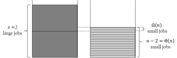
Figure 1: The 4/3 approximation local optimum of $P^{*}_{\epsilon}$ [22]

3 Generalised Worst-Case Instance

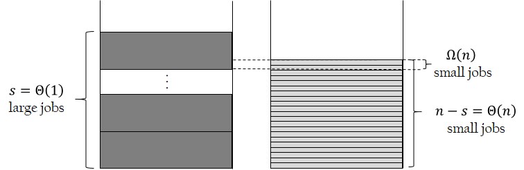
Figure 2: A local optimum of $G^{*}_{\epsilon}$

The instance from the literature $P^{*}_{\epsilon}$ leading to a 4/3 worst-case expected approximation ratio for RLS and the $(1+1)~{}\text{EA}$ consists of two large jobs with long processing times $p_{1}:=p_{2}:=1/3-\epsilon/4$ and the remaining $n-2$ jobs with short processing times $p_{i}:=(1/3+\epsilon/2)/(n-2)$ for $3\leq i\leq n$ (the sum of the processing times are normalised to 1 for cosmetic reasons) [22]. Any partition where one large job and half of the small jobs are placed on each machine is naturally a global optimum of the instance (i.e., the makespan is 1/2). Note that the sum of all the processing times of the small jobs is slightly larger than the processing time of a large job. The local optimum leading to the 4/3 expected approximation consists of the two large jobs on one machine and all the small jobs on the other. It is depicted in Figure 1. The makespan of the local optimum is $p_{1}+p_{2}=2/3-\epsilon/2$ and, in order to decrease it, a large job has to be moved to the fuller machine and at the same time at least $\Omega(n)$ small jobs have to be moved to the emptier machine. Since this requires to flip $\Omega(n)$ bits, which cannot happen with RLS and only happens with exponentially small probability $n^{-\Omega(n)}$ with the SBM of EAs, their expected runtime to escape from such a configuration is at least exponential.

In this section, to highlight the power of the AIS to overcome hard local optima for EAs, we generalise the instance $P^{*}_{\epsilon}$ to contain an arbitrary number $s=\Theta(1)$ of large jobs and show how the considered AISs efficiently solve the instance class to optimality by escaping from local optima efficiently while RLS and the $(1+1)~{}\text{EA}$ cannot. Hence, hypermutations and ageing are efficient at locating the optimal solution on a vast number of instances where SBM and local mutations alone fail. The generalised instance class $G^{*}_{\epsilon}$ is defined as follows.

Definition 2.

The class of Partition instances $G^{*}_{\epsilon}$ are characterised by an even number of jobs $n$, an even number of large jobs $s=\Theta(1)$ and the following processing times:

$$p_{i}=\begin{cases}\frac{1}{2s-1}-\frac{\epsilon}{2s}&\text{if }i\leq s,\\ \frac{s-1}{n-s}\cdot(\frac{1}{2s-1}+\frac{\epsilon}{2(s-1)})&\text{otherwise,}\end{cases}$$

where $0<\epsilon<1/(2s-1)$ is an arbitrarily small constant.

The instance class has the same property as the instance $P^{*}_{\epsilon}$. If all the large jobs are placed on one machine and all the small jobs on the other, then at least $\Omega(n)$ small jobs need to be moved in exchange for a large job to decrease the discrepancy (the difference between the loads of the machines). Such a local optimum allows to derive a lower bound on the worst-case expected approximation ratio of algorithms that get stuck there. Obviously the greater the number of large jobs, the smaller the bound on the approximation ratio will be. Next, we will point out some important characteristics of the instance class. In particular, we will provide upper bounds on the number of distinct makespan values that can be observed; first for all possible solutions and then only among local optima. Finally, we will provide restrictions on the distribution of the small jobs among the machines which hold for all suboptimal solutions.

Property 1.

Let $x\in\{0,1\}^{n}$ be a solution to the instance $I\in$ $G^{*}_{\epsilon}$, $h$ and $k$ be the numbers of large and small jobs respectively on the fuller machine of $x$ and $\mathcal{L}\subseteq\{0,1\}^{n}$ be the set of local optima of $I$. Then,

1. $|\{y\in\mathbb{R}:\exists x\in\{0,1\}^{n}\;\text{s.t.}\;f(x)=y\}|=O(n)$

2. $|\{y\in\mathbb{R}:\exists x\in\mathcal{L}\;\text{s.t.}\;f(x)=y\}|=O(1)$

3. $\forall x\in\{0,1\}^{n}$ s.t. $f(x)>1/2$, either $k=\Omega(n)$ and $x\notin\mathcal{L}$, or $\max(k,n-s-k)\geq\left(\frac{1}{2}+a\right)(n-s)$ for some $a=\Omega(1)$.

Proof.

Since $p_{i}=p_{j}=p_{1}$ for all $(i,j)\in[s]^{2}$ and $p_{i}=p_{j}=p_{s+1}$ for all $(i,j)\in([n]\setminus[s])^{2}$, $f(x)=h\cdot p_{1}+k\cdot p_{s+1}.$ The first property follows from $(h,k)\in[s]\times[n-s]$ and $s=O(1)$.

For the second property which considers only the local optima $\mathcal{L}$, note that if a local optimum $\ell$ with $h$ large jobs and $k$ small jobs exists, then a solution which has $h$ large jobs and $k^{\prime}<k$ small jobs on its fuller machine cannot exist since, otherwise, moving a small job to the emptier machine would improve $\ell$. Moreover, any solution with $h$ large jobs and $k^{\prime}>k$ small jobs on its fuller machine cannot be a local optima since it can be improved by moving a small job from its fuller machine to its emptier machine. Thus, there exists a unique locally optimal makespan value for each $h\in[s]$. The property follows from $s=O(1)$.

In order to show the third property, we will partition the set of suboptimal solutions $\mathcal{X}\subset\{0,1\}^{n}$ into three disjoint sets:

• $\mathcal{X}_{1}:=\{x\in{\mathcal{X}}:f(x)\geq\sum_{i=1}^{s}p_{i}+\left(\frac{1}{s+1}\sum_{i=s+1}^{n}p_{i}\right)\}$,

• $\mathcal{X}_{2}:=\{x\in{\mathcal{X}}\setminus\mathcal{X}_{1}:h<s\wedge x\notin\mathcal{L}\}$ ,

• $\mathcal{X}_{3}:={\mathcal{X}}\setminus(\mathcal{X}_{1}\cup\mathcal{X}_{2})$,

for all $x\in\mathcal{X}_{1}$, since $f(x)\geq\sum_{i=1}^{s}p_{i}+\left(\frac{1}{s+1}\sum_{i=s+1}^{n}p_{i}\right)>\frac{1}{2}+\frac{1}{s+1}\sum_{i=s+1}^{n}p_{i}$, moving a single small job from the fuller machine to the emptier machine always improves the makespan, thus $x\notin\mathcal{L}$. Moreover, since the sum of the processing times of the large jobs on the fuller machine can be at most $\sum_{i=1}^{s}p_{i}$, we get $k\geq(n-s)/(s+1)=\Omega(n)$.

For any $x\in\mathcal{X}_{2}$, $x\notin\mathcal{L}$ by definition. We will prove by contradiction that $k=\Omega(n)$. Let us assume $k=o(n)$. Since the condition $h<s$ implies that there is at least one large job in the emptier machine, the load of the emptier machine is at least

$$f(x) \geq\left(\frac{1}{2s-1}-\frac{\epsilon}{2s}\right)+(n-s-o(n))\cdot\frac{s-1}{n-s}\left(\frac{1}{2s-1}+\frac{\epsilon}{2\left(s-1\right)}\right)(1-o(1))$$

$$\geq\frac{1}{2}\left(1+\frac{1}{2s-1}+\frac{(s-1)\epsilon}{s}\right)(1-o(1))>\frac{1}{2}\;\ \text{(for large enough $n$)},$$

and contradicts that it is the emptier machine. Thus, $k=\Omega(n)$.

Finally, we will show that for all $x\in\mathcal{X}_{3}$, $\max(k,n-s-k)\geq\left(\frac{1}{2}+a\right)n$ for some $a=\Omega(1)$. When $x\in\mathcal{X}_{3}$ and $h=s$, then $k<\frac{n-s}{s+1}$ since $f(x)<\sum_{i=1}^{s}p_{i}+\left(\frac{1}{s+1}\sum_{i=s+1}^{n}p_{i}\right)$. The inequality $k<\frac{n-s}{s+1}$ in turn implies that $n-s-k>(n-s)-\frac{n-s}{s+1}=(n-s)(1-(1/(s+1)))\geq(1/2+a)n$ for some $a$. If $x\in\mathcal{X}_{3}$ and $x\in\mathcal{L}$, then either there are no small jobs on the fuller machine ($k=0$), or the difference between the loads is so small that moving a small job to the emptier machine does not improve the makespan. For the latter case, since $f(x)>\frac{1}{2}$, the machines cannot have the same number of small and large jobs. Moreover, since $s$ and $n$ are even intergers and $x\in\mathcal{L}$, if one of the machines has more than half of the large (small) jobs assigned to it, then more than half of the small (large) jobs has to be assigned to the other machine, because otherwise moving a single small job from the fuller machine to the emptier one would improve the makespan. Without loss of generality (w.l.o.g.), let $M_{1}$ be the machine with more small jobs and fewer large jobs. Since $\sum_{i=1}^{n}p_{i}=1$, the load of $M_{1}$ is at least $1/2-p_{s+1}/2$. By definition, the number of large jobs in $M_{1}$, is bounded above by $s/2-1$. Then, the contribution of small jobs to the load of $M_{1}$ is at least

$$\frac{1}{2}\left(s\cdot p_{1}+(n-s)p_{s+1}-p_{s+1}\right)-\left(\frac{s}{2}-1\right)p_{1}=\frac{n-s-1}{2}p_{s+1}+p_{1},$$

where the first expression makes use of $s\cdot p_{1}+(n-s)p_{s+1}=1$. We can divide by $p_{s+1}$ and establish that the number of small jobs is at least:

$$\frac{n-s-1}{2}+\frac{p_{1}}{p_{s+1}}>\frac{n-s-1}{2}+\frac{n-s}{s}=(n-s)\left(\frac{1}{2}+\frac{1}{s}\right)\left(1-O\left(\frac{1}{n}\right)\right).$$

Thus, for all $x\in\mathcal{X}_{3}$, $\min{(k,n-s-k)}\geq(n-s)(\frac{1}{2}+a)$ where $a:=\min{(\frac{1}{s}-O(\frac{1}{n}),\frac{1}{2}-\frac{1}{s+1})}=\Omega(1)$. ∎

We now prove that the $(1+1)~{}\text{EA}$ has exponential expected runtime on $G^{*}_{\epsilon}$. The proof is similar to that of the 4/3 approximation [22]. It essentially shows that with constant probability the algorithm gets trapped in a state where it is exponentially unlikely to move the extra large jobs out of its fuller machine. That RLS also fails is essentially a corollary.

Theorem 2.

The $(1+1)~{}\text{EA}$ needs at least $n^{\Omega(n)}$ fitness function evaluations in expectation to optimise any instance of $G^{*}_{\epsilon}$.

Proof.

The proof is similar to that of the 4/3 approximation [22]. We will first prove that with constant probability the $(1+1)~{}\text{EA}$ initialises with all large jobs in $M_{1}$ and then fills $M_{2}$ with a $(1-\frac{\epsilon}{2(s-1)})$ fraction of the small jobs before moving any large jobs to $M_{2}$ (Event $\mathcal{E}_{1}$). From then on, we will show that the algorithm requires exponential expected time to move a large job. Since the sum of the processing times of large jobs is larger than $1/2$ (the makespan of the optimum), the expected optimisation time will be exponential as well.

With probability $(1/2)^{s}=\Theta(1)$, all large jobs are assigned to the same machine ($M_{1}$ w.l.o.g.) in the initial solution. The expected number of small jobs initially assigned to $M_{1}$ is $(n-s)/2$ and since they are assigned independently, the probability that more than $(n/2)+n^{3/5}$ of them are assigned is exponentially small due to Chernoff bounds.

Let $k_{t}$ be the number of small jobs on the fuller machine $M_{1}$ at time $t$. As long as the large jobs are not moved, new solutions are only accepted if the number of small jobs in $M_{2}$ increases or stays the same. A single small job is moved to $M_{2}$ with probability $(k_{t}/n)(1-1/n)^{n-s-1}\geq k_{t}/(en)$.

The expected time conditional on large jobs never having been moved until a $(1-\frac{\epsilon}{2(s-1)})$ fraction of the small jobs are moved to $M_{2}$ is:

$$\sum_{k=\epsilon(n-s)/(2(s-1))}^{n/2+n^{3/5}}\frac{en}{k} \leq en\sum_{k=\epsilon(n-s)/(2(s-1))}^{n/2+n^{3/5}}\frac{2(s-1)}{\epsilon\left(n-s\right)}$$

$$\leq 2(s-1)\left(\frac{e}{\epsilon}\right)\left(\frac{n}{n-s}\right)\left(\frac{n}{2}+n^{3/5}\right)$$

$$\leq 2(s-1)\frac{e}{\epsilon}\frac{n}{2}\left(1+o(1)\right)\leq O(n)$$

Let $c$ be a constant such that $cn-1$ is at least twice as large as the above expectation. Due to Markov’s inequality at least a $(1-\frac{\epsilon}{2(s-1)})$ fraction of the small jobs are moved to $M_{2}$ in $cn-1$ iterations with probability at least $1/2$. Now, we calculate the probability that no large jobs have been moved in $cn-1$ iterations. The probability that SBM does not move any large jobs to the emptier machine ($M_{2}$) is $1-s/n$ in each iteration. The probability that the large jobs are not moved during the first $cn-1$ iterations is at least $(1-s/n)^{cn-1}\geq e^{-cs}=\Omega(1)$. Hence, Pr$\{\mathcal{E}_{1}\}=\Omega(1)$.

Now that we found the probability of event $\mathcal{E}_{1}$, we can find the expected runtime conditional on $\mathcal{E}_{1}$.

Let at least a $(1-\frac{\epsilon}{2(s-1)})$ fraction of small jobs and all the large jobs be on $M_{2}$. The sum of the processing times of small jobs on $M_{2}$ is greater than the processing time of ($s-1$) large jobs (i.e., $\frac{s-1}{2s-1}-\frac{\epsilon}{2}\frac{s-1}{s}$) and greater than

$$(s-1)\left(\frac{1}{2s-1}+\frac{\epsilon}{2(s-1)}\right)-\frac{\epsilon}{2}\left(\frac{1}{2s-1}+\frac{\epsilon}{2(s-1)}\right)$$

$$=\frac{s-1}{2s-1}+\frac{\epsilon}{2}\bigg{(}1-\frac{1}{2s-1}-\frac{\epsilon}{2(s-1)}\bigg{)}{\color[rgb]{0,0,0}>\frac{s-1}{2s-1}+\frac{\epsilon}{3}-\frac{\epsilon^{2}}{4}>\frac{s-1}{2s-1}+\frac{\epsilon}{4}.}$$

Then the makespan can be at most $S<1-\big{(}\frac{s-1}{2s-1}+\frac{\epsilon}{4}\big{)}=\frac{s}{2s-1}-\frac{\epsilon}{4}$. If a large job was to be transferred to $M_{2}$, then its total time would become $S^{\prime}>\frac{s}{2s-1}+\frac{\epsilon}{4}-\frac{\epsilon}{2s}>\frac{s}{2s-1}$. Hence, in order for a large job to be transferred to $M_{2}$, a processing time of at least $\epsilon/4$ has to be transferred to $M_{1}$ in the same iteration. Then the conditional expected time to transfer a large job would be exponential since at least a linear number of small jobs need to be moved from $M_{2}$ to $M_{1}$ such that their processing times of order $O(1/n)$ sum up to a constant $\epsilon/4$. Such a mutation requires at least a linear number of bits to be flipped which happens with probability at most $n^{-\Omega(n)}$. The probability that such a mutation happens in $n^{\delta n}$ steps is still in the same asymptotic order for a sufficiently small constant $\delta$. Since any mutation that increases the load of $M_{2}$ will not be accepted and the large jobs must be equally distributed among the machines in the optimal solution, with $\text{Pr}\left\{\mathcal{E}_{1}\right\}\cdot(1-n^{-\Omega(n)})=\Omega(1)$ the runtime will be in the order of $n^{\Omega(n)}$. The theorem statement follows since $E(T)\geq E(T\mid\mathcal{E}_{1})\cdot\text{Pr}\{\mathcal{E}_{1}\}=n^{\Omega(n)}$ by the definition of expectation of a random variable. ∎

In the following subsection, we will show that hypermutations are efficient. Afterwards we will do the same for ageing.

3.1 Hypermutations

We will start this subsection by proving some general statements about hypermutations. The hypermutation operator flips all the bits in a bitstring successively and evaluates the fitness after each step. Unless an improvement is found first, each hypermutation operation results in a sequence of $n$ solutions sampled in the search space. This sequence of solutions contains exactly one bitstring for each Hamming distance $d\in[n]$ to the initial bitstring. Moreover, the string which will be sampled at distance $d$ is uniformly distributed among all the bitstrings of distance $d$ to the input solution.

The number of possible outcomes grows exponentially in the number of flipped bits until the ($n/2$)th bit is flipped and afterwards reduces at the same rate. Thus, the first and the last constant number of sampled strings are picked among a polynomially large subset of the search space. We will now provide a lemma regarding the probability of particular outcomes in the first and the last $m$ bitstrings of the sequence.

Lemma 3.

Let $x^{i}\in\{0,1\}^{n}$ be the $i_{th}$ bitstring sampled by the hypermutation and for any arbitrary subset of indices $S\subset[n]$, let $x^{i}_{S}$ be the subsequence of $x^{i}$ which consists of bit positions in $S$. For any given target string $s^{*}\in\{0,1\}^{|S|}$ and integer $m>|S|$, the probability that $\forall i\in\{m,\ldots,n-m\}$, $x^{i}_{S}=s^{*}$ is at least $\left(\frac{m-|S|+1}{n-|S|+1}\right)^{|S|}$.

Proof.

Let $S_{A}$ and $S_{D}$ denote the set of positions where the initial subsequence $x^{0}_{S}$ and $s^{*}$ agree and disagree respectively and $ord(j)\in[n]$ denote the mutation step when the bit position $j\in S$ is flipped. Then, $\forall i\in\{m,\ldots,n-m\},\enskip x^{i}_{S}=s^{*}$ holds if and only if $\forall j\in S_{D},\enskip ord(j)\leq m$ and $\forall j\in S_{A},\enskip ord(j)\geq n-m$. Given that there are at least $k$ different $j\in S_{D}$ such that $\enskip ord(j)\leq m$, the probability that there are at least $k+1$ different $j\in S_{D}$ such that $\enskip ord(j)\leq m$ is $(m-k)/(n-k)$. Thus, the probability that $\enskip ord(j)\leq m$ holds for all $j\in S_{D}$ is at least $\prod_{k=0}^{|S_{D}|-1}\frac{m-k}{n-k}$. Similarly, if $\enskip ord(j)\leq m$ holds for all $j\in S_{D}$ and there are at least $k$ different $j\in S_{A}$ such that $\enskip ord(j)\geq n-m$, the probability that there are at least $k+1$ different $j\in S_{A}$ such that $\enskip ord(j)\geq n-m$ is at least $(m-k)/(n-k-|S_{D}|)$. Thus, the probability that, $\forall j\in S_{D},\enskip ord(j)\leq m$ and $\forall j\in S_{A},\enskip ord(j)\geq n-m$ is at least $\left(\prod_{k=0}^{|S_{D}|-1}\frac{m-k}{n-k}\right)\left(\prod_{k=0}^{|S_{A}|-1}\frac{m-k}{n-k-|S_{D}|}\right)\geq\left(\frac{m-|S|+1}{n-|S|+1}\right)^{|S|}$. ∎

We can observe that the probability bounds we get from this lemma are polynomial if $|S|$ is a constant. Moreover, if both $|S|=\Theta(1)$ and $m=\Omega(n)$ we obtain probabilities in the order of $\Omega(1)$.

For $G^{*}_{\epsilon}$, we would like to distribute two kinds of jobs evenly among the machines. While one type of job is constant in number, the other is in the order of $\Theta(n)$. So the previous lemma would provide reasonable probability bounds only for the large jobs. For the small jobs we will make use of the fact that the configuration we want is not any configuration, but an exact half and half split. Intuitively, it is obvious that if all the jobs start on one machine, at exactly the $\frac{n}{2}$th bit flip the split will be half and half. However, as the starting distribution gets further away from the extremes, it becomes less clear when the split will exactly happen. Fortunately, the fact that the number of small jobs is large will work in our favor to predict the time of the split more precisely.

Theorem 3.

If the input bitstring of hypermutation has $\left(\frac{1}{2}+a\right)n$ 1-bits for some constant $a>0$, then with probability $1-e^{-\Omega(nc^{2})}$, for any $c=\omega(\sqrt{\log{n}/n})$ such that $c\in(0,a)$, there exists a $k\in\{n\frac{a-c}{2a-c},\ldots,n\frac{a}{2a-c}\}$, such that the number of 1-bits in the $k_{th}$ solution sampled by hypermutation has exactly $n/2$ 1-bits.

Proof.

Let $Y_{k}$ be the total number of 1-bits flipped by the hypermutation operator up to and including the $k$th mutation step. Given any parent string $x\in\{0,1\}^{n}$ with $\left(\left(1/2\right)+a\right)n$ $1$-bits, $Y_{k}$ is a hypergeometrically distributed random variable with parameters $n$, $\left(\left(1/2\right)+a\right)n$, $k$ and expectation $E[Y_{k}]=\left(\left(1/2\right)+a\right)\cdot k$.

Let $X_{k}$ be the bit-string sampled after the $k$th mutation step. It has $\left(\left(1/2\right)+a\right)n-Y_{k}$ of $x$’s $1$-bits which have never been flipped and $k-Y_{k}$ of its $0$-bits which are flipped to $1$-bits. Thus, the number of 1-bits in $X_{k}$, $|X_{k}|_{1}=\left(\left(1/2\right)+a\right)n+k-2Y_{k}$. Now, we can bound the probability that $|X_{k}|_{1}\geq n/2$ after a particular mutation step $k\geq\frac{n\cdot a}{2a-c}$ by using Theorem 1.

$$\text{Pr}\left\{|X_{k}|_{1}>n/2\right\} =\text{Pr}\left\{Y_{k}<\frac{k+a\cdot n}{2}\right\}=\text{Pr}\left\{Y_{k}<\frac{k+a\cdot n}{k+2a\cdot k}\cdot E[Y_{k}]\right\}$$

$$\leq\text{Pr}\left\{Y_{k}<\left(1-\frac{c}{2a+1}\right)\cdot E[Y_{k}]\right\}\leq\exp{\left(-\left(\frac{c}{1+2a}\right)^{2}\frac{E[Y_{k}]}{2}\right)}$$

$$\leq\exp{\left(-\left(\frac{c}{1+2a}\right)^{2}\frac{\left(\frac{1}{2}+a\right)\frac{n\cdot a}{2a-c}}{2}\right)}=e^{-\Omega(nc^{2})},$$

where we used $k\geq\frac{n\cdot a}{2a-c}$ to obtain the first and the last inequality and Theorem 1 to obtain the second. Then, using the same line of arguments, we bound $\text{Pr}\left\{|X_{k}|_{1}<n/2\right\}$ at any given mutation step $k\leq n\frac{n\cdot(a-c)}{2a-c}$ by $e^{-\Omega(nc^{2})}$:

$$\text{Pr}\left\{|X_{k}|_{1}<n/2\right\} =\text{Pr}\left\{Y_{k}>\left(1+\frac{a\cdot c}{(2a+1)(a-c)}\right)\cdot E[Y_{k}]\right\}$$

$$\leq\exp{\left(-\left(\frac{a\cdot c}{(2a+1)(a-c)}\right)^{2}\frac{E[Y_{k}]}{3}\right)}\leq e^{-\Omega(nc^{2})},$$

where in the last inequality we used that $a/(2a+1)=\Omega(1)$ and that $(a-c)=o(1)$ only when $c=\Omega(1)$. Finally, we will use the union bound and the $c=\omega\left(\sqrt{\frac{\log{n}}{n}}\right)$ assumption to prove our claim.

$$\text{Pr}\left\{\forall k\in\left[\frac{n\cdot(a-c)}{2a-c},\frac{n\cdot a}{2a-c}\right]:|X_{k}|_{1}\neq n/2\right\}$$

$$\leq\sum\limits^{n}_{j=\frac{n\cdot a}{2a-c}}\text{Pr}\left\{|X_{j}|_{1}>n/2\right\}+\sum\limits^{\frac{n\cdot(a-c)}{2a-c}}_{j=1}\text{Pr}\left\{|X_{j}|_{1}<n/2\right\}\leq n\cdot e^{-\Omega(nc^{2})}=e^{-\Omega(nc^{2})}.$$

∎

Now we have all the necessary tools to prove that the $(1+1)~{}\text{IA}^{hyp}$ can solve $G^{*}_{\epsilon}$ efficiently. To prove our result, we will use the combination of Property 1.3, Lemma 3, and Theorem 3 to show that the probability of improvement is at least $\Omega(1)$ for any suboptimal solution and then obtain our bound on the expected runtime by Property 1.1, which indicates that there can be at most $O(n)$ improvements before the optimum is found. The heart of the proof of the following theorem is to show that from any local optimum, hypermutations identify the global optimum with constant probability unless an improvement is found first.

Theorem 4.

The $(1+1)~{}\text{IA}^{hyp}$ optimises the $G^{*}_{\epsilon}$ class of instances in $O(n^{2})$ expected fitness function evaluations.

Proof.

According to Property 1.3, for any suboptimal solution $x$, either there are at least a linear number of small jobs that can be moved from the fuller machine to the emptier machine to improve the makespan or the number of small jobs in each machine differs from $\frac{n-s}{2}$ by a linear factor.

For the former case, in the first mutation step the probability that hypermutation flips one of the bits which correspond to the small jobs in the fuller machine is at least $\Omega(n)/n=\Omega(1)$. Since such a mutation creates an improved solution, the hypermutation operator stops and the overall improvement probability is at least $\Omega(1)$.

For the latter case, the number of small jobs in one of the machines is at least $\left(\frac{1}{2}+a\right)(n-s)$ for some positive constant $a$. Using the notation of Theorem 3 with $a$ and $c=1/(a\log{n})$, with overwhelming probability the number of small jobs assigned to each machine will be exactly $(n-s)/2$ at some bit-flip between $(n-s)\frac{(a)-1/(a\log{n})}{(2/a)-1/(a\log{n})}=(n-s)\frac{1-(1/\log{n})}{2-1/\log{n}}$ and $(n-s)\frac{a}{(2a)-1/(a\log{n})}=(n-s)\frac{1}{2-1/(\log{n})}$. According to Lemma 3, the probability that the large jobs are distributed evenly throughout this interval is at least:

$$\left(\frac{(n-s)\frac{1-(1/\log{n})}{2-(1/\log{n})}-s+1}{n-s+1}\right)^{s}=2^{-s}(1-o(1))=\Omega(1).$$

Therefore, with probability $\Omega(1)$ either the optimal solution will be found or the hypermutation will stop due to an improvement. Since according to Property 1.1 there are at most $O(n)$ different makespan values and the probability of improvement is at least $\Omega(1)$ for all sub-optimal solutions, the optimum is found in expected $O(n)$ iterations. Given that the hypermutation operator evaluates at most $n$ solutions in each iteration, our claim follows. ∎

Since the worst case instance for the $(1+1)~{}\text{EA}$ presented in [22] is an instance of $G^{*}_{\epsilon}$ with $s=2$, the following corollary holds.

Corollary 1.

The $(1+1)~{}\text{IA}^{hyp}$ optimises $P_{\epsilon}^{*}$ in $O(n^{2})$ expected fitness function evaluations.

3.2 Ageing

In this section we will show that the $(\mu+1)~{}\text{EA}^{ageing}$ can optimise the $G^{*}_{\epsilon}$ instances efficiently. Our approach to prove the following theorem is to first show that if a solution where the large jobs are equally distributed is sampled in the initialisation, then it takes over the population and the $(\mu+1)~{}\text{EA}^{ageing}$ quickly finds the optimum. The contribution of ageing is considered afterwards to handle the case when no such initial solution is sampled. Then we will show that whenever the algorithm gets stuck at a local optima, it will reinitialise the whole population after $\tau$ iterations and sample a new population. Before we move to the main results, we will prove two helper lemmata. In the first lemma, we will closely follow the arguments of Lemma 5 in [26] to get a similar but more precise bound.

Lemma 4.

Consider a population of the $(\mu+1)~{}\text{EA}^{ageing}$ which consists of solutions of equal fitness. Given that no improvement is found and no solutions reach age $\tau$ before, the expected time until the population consists of solutions with the same age is at most $144\mu^{3}$.

Proof.

Let $X_{t}$ denote the largest number of individuals in the population having the same age. While $X_{t}<\mu$, the number of individuals increases if one of the $X_{t}$ individuals is selected as parent, the SBM does not flip any bits and a solution from another age group is removed from the population.

$$\text{Pr}\left\{X_{t+1}=X_{t}+1\mid X_{t}\right\}\geq\frac{X_{t}(\mu-X_{t})}{\mu(\mu+1)}\cdot\left(1-\frac{1}{n}\right)^{n}$$

Similarly, $X_{t}$ decreases only if a solution from another age group is cloned and one of the $X_{t}$ solutions are removed from the population.

$$\text{Pr}\left\{X_{t+1}=X_{t}-1\mid X_{t}\right\}\leq\frac{(\mu-X_{t})X_{t}}{\mu(\mu+1)}\cdot\left(1-\frac{1}{n}\right)^{n}\leq\text{Pr}\left\{X_{t+1}=X_{t}+1|X_{t}\right\}$$

Let a relevant step be any iteration where $X_{t}\neq X_{t+1}$. Then, the number of generations where $X_{t+1}\geq X_{t}$ in $2\mu^{2}$ relevant steps has a distribution that stochastically dominates the binomial distribution with parameters $2\mu^{2}$ and $1/2$. Since for any random variable $X\sim Bin(2\mu^{2},1/2)$, $\text{Pr}\left\{X\geq\mu^{2}+\frac{1}{2}\sqrt{\mu^{2}}\right\}\geq\frac{1}{8}$ (Lemma 1), the probability that $X_{t}$ increases at least $\mu^{2}+\mu/2$ times in a phase of $2\mu^{2}$ relevant steps is at least $1/8$. Since $X_{t}\geq 1$, the expected number of relevant steps until $X_{t}=\mu$ is at most $(1/8)^{-1}2\mu^{2}=16\mu^{2}$. The probability of a relevant step is at least

$$\frac{(\mu-X_{t})X_{t}}{\mu(\mu+1)}\cdot\left(1-\frac{1}{n}\right)^{n}\geq\frac{(\mu-1)}{\mu(\mu+1)}\cdot\left(1-\frac{1}{n}\right)^{n}\geq\frac{1}{3\mu}\cdot\frac{1}{3}=\frac{1}{9\mu},$$

for any $\mu\geq 2$ and $n\geq 3$. Thus, the expected waiting time for a relevant step is at most $9\mu$ and the total expected time until the population reaches the same age is at most $144\mu^{3}$. ∎

Lemma 5.

For any partition instance with $L$ local optima with different makespans, the expected time until the $(\mu+1)~{}\text{EA}^{ageing}$ with $\mu=O(\log{n})$ and $\tau=O(n^{1+c})$ for any constant $c$ either reinitialises the population or finds the optimum is at most $L(2en^{2}+\tau)(1+o(1))$.

Proof.

Let $X_{t}$ denote the solution with the smallest makespan in the population at time $t$. Starting from any current population, consider a phase of length $c^{\prime}L(n^{2}+\tau)$ for some constant $c^{\prime}>3e$. We will make a case distinction with respect to whether the following statement holds during the entirety of the phase.

$$\forall t\enskip X_{t}\in\mathcal{L}:\exists t^{\prime}\leq t+\tau+145\mu^{4}\text{ s.t. }f(X_{t^{\prime}})<f(X_{t})$$

The statement indicates that whenever a local optimum becomes the best solution in the population, a solution with a better makespan is found in at most $\tau+145\mu^{4}$ iterations.

Case 1: If the statement holds throughout the phase then, at most $L(\tau+144\mu^{4})=O(L\cdot\tau)$ iterations satisfy $X_{t}=\ell_{i}$ for some $i$. Since the $(\mu+1)~{}\text{EA}^{ageing}$ with $f(\ell_{i})>f(X_{t})\geq f(\ell_{i+1})$ samples a solution $x$ with $f(x)\leq f(\ell_{i+1})$ in $2en^{2}(1+o(1))$ iterations with probability at least $1-n^{-\Omega(n^{c})}$ according to Lemma 2, by the union bound the total number of iterations during the phase where the current best solution is not a local optimum is at most $L\cdot 2en^{2}\cdot(1+o(1))$ with probability at least $1-n^{-\Omega(n^{c})}\cdot 2^{n}=1-o(1)$. Therefore, in $L\cdot 3en^{2}$ iterations the optimal solution is found with at least constant probability.

Case 2: If the statement does not hold for some $t$, then there exists a time interval of length $\tau+145\mu^{4}$ during the phase where no improvements will occur and the current best individual is a local optimum. Given that there are $k$ individuals which share the best fitness value, with probability $(k/\mu)(1-1/n)^{n}\geq(k/\mu)(1-1/n)e^{-1}$, SBM creates a copy of one of these solutions. Since the fitness cannot be improved by our assumption, in at most $\sum_{k=1}^{\mu}(\mu/k)(1-1/n)^{-1}e=(1+o(1))e\mu\ln{\mu}$ expected time the population only consists of individuals with the best fitness. This occurs in less than $2e\mu\ln{\mu}$ iterations with probability at least $1/3$ due to Markov’s inequality. According to Lemma 4, unless the best fitness is improved, in at most $144\mu^{3}$ steps the population reaches the same age. Using Markov’s inequality, we can bound the probability that this event happens in at most $145\mu^{3}$ iterations by $\Omega(1)$ from below. Thus, given that the best fitness does not improve in $\tau+145\mu^{4}$ iterations, in $2e\mu\ln{\mu}+145\mu^{3}$ iterations, the population consists of solutions with the same fitness and the same age with constant probability, which leads to a reinitialisation before the phase ends.

If neither the optimal solution is found nor the population is reinitialised, we repeat the same argument starting from an arbitrary population. Since, the probability of at least one of the events happenning is constant, in a constant expected number of phases of length $L(\tau+145\mu^{4})=L\cdot\tau(1+o(1))$, one of the events occurs. ∎

We will now show that with probability at least $p_{success}=\Omega(1)$, the optimal solution will be found in $O(n^{3/5})$ iterations starting from a randomly initialised population. Since Lemma 5 and Property 1.2 imply that the expected time until either the optimum is found or the population is reinitialised is in the order of $O(n^{2}+\tau)$, in $O(n^{3/5})+O(n^{2}+\tau)/p_{success}=O(n^{2}+\tau)$ expected iterations the optimum is found.

Theorem 5.

The $(\mu+1)~{}\text{EA}^{ageing}$ optimises the $G^{*}_{\epsilon}$ class of instances in $O(n^{2}+\tau)$ steps in expectation for $\tau=\Omega(n^{1+c})$ for any arbitrarily small constant $c$ and $\mu=O(\log{n})$.

Proof.

With probability $\binom{s}{s/2}2^{-s}{\color[rgb]{0,0,0}=\Omega(1)}$, a randomly initialised solution assigns an equal number of large jobs to each machine. We will refer to such solutions as good solutions. For any initialised individual, the expected number of small jobs assigned to each machine is $(n-s)/2$. By Chernoff bounds (Theorem 1), the probability that less or more than $(n/2)\pm n^{3/5}$ small jobs are assigned to one machine is $e^{-\Omega(n^{1/5})}$. We will now show that if there is at least one good individual at initialisation, then in $O(\mu\log{\mu})$ generations, the whole population will consist of good solutions with at least constant probability.

For a bad (not good) initial solution, the difference between the number of large jobs in $M_{1}$ and $M_{2}$ is at least $2$ by definition. With $1-e^{-\Omega(n^{1/5})}$ probability, the initial number of small jobs assigned to each machine will not differ by more than $O(n^{3/5})$ (event $\mathcal{E}_{2}$) . Thus, the difference between the loads of the machines is at least $\Omega(1)$ for a bad solution, while less than $O(n^{-2/5})$ for a good one, both with overwhelmingly high probabilities. In order for a bad solution to have a better fitness than a good one, it is necessary that at least $\Omega(n)$ small jobs are moved from the fuller machine to the emptier machine which takes at least $\Omega(n/\log{n})$ time with overwhelmingly high probability since the probability of SBM flipping more than $\log{n}$ bits is exponentially small.

If there are $k$ good solutions in the population, the probability that one of them is selected as parent is $k/\mu$ and the probability that SBM does not flip any bits and yields a copy is $(1-(1/n))^{n}>1/3$. Thus, the expected time until the good solutions take over the population is at most $3\mu\sum_{k=1}^{\mu}(1/k)\leq 3\mu\ln{\mu}$. The probability that the good solutions take over the population in at most $O(n^{3/5})$ iterations (before any bad solution is improved to a fitness value higher than the initial fitness of a good solution) is by Markov’s inequality in the order of ${\color[rgb]{0,0,0}1-}O((\log{n})(\log{\log{n}})/n^{3/5})$. Thus, if the initial population contains at least one good solution, it takes over the population with probability $1-o(1)$. Moreover, since the discrepancy (the difference between the loads of the machines) of the accepted good solutions will not increase above $\Omega(n^{-2/5})$, SBM needs to move a linear number of small jobs in a single iteration to create a bad solution from a good one, which does not happen with probability at least $1-n^{-\Omega(n)}$.

Starting from a suboptimal good solution, the fitness improves by moving any small job from the fuller machine to the emptier machine without moving any of the large jobs. The probability of such an event is at least $(n-s)/2n\cdot(1-1/n)^{n-1}=\Omega(1)$ considering that there are at least $(n-s)/2n$ small jobs on the fuller machine. Since the difference between the number of small jobs is in the order $O(n^{3/5})$, the small jobs will be distributed exactly evenly and the global optimum will be reached in expected $O(n^{3/5})$ iterations. Using Markov’s inequality, we can bound the probability that global optimum will be reached in $O(n^{3/5})$ iterations by $\Omega(1)$.

Since all necessary events described for finding the optimum have at least probability $\Omega(1)$, the probability that they occur in the same run is at least in the order of $\Omega(1)$ as well. Thus, all that remains is to find the expected time until the population consists of $\mu$ randomly initialised individuals given that one of the necessary events fails to occur and the global optimum is not found. This expectation is at most $L\cdot(2en^{2}+\tau)(1+o(1))$ due to Lemma 5 with $L=\Omega(1)$ which is in turn due to Property 1.2. Thus, our expectation is $(1/p_{success})\cdot O(n^{2}+\tau)+O(n^{3/5})=O(n^{2}+\tau)$. ∎

Clearly the following corollary holds as $P_{\epsilon}^{*}$ is an instance of $G^{*}_{\epsilon}$.

Corollary 2.

The $(\mu+1)~{}\text{EA}^{ageing}$ optimises $P_{\epsilon}^{*}$ in $O(\mu n^{2}+\tau)$ steps in expectation for $\tau=\Omega(n^{{\color[rgb]{0,0,0}1+c}})$ and $\mu=O(\log n)$.

4 $(1+\epsilon)$ Approximation Ratios

In this section we will show that both the $(1+1)~{}\text{IA}^{hyp}$ and the $(\mu+1)~{}\text{EA}^{ageing}$ are polynomial time approximation schemes, i.e., they guarantee solutions with makespan at most a $(1+\epsilon)$ factor worse than the optimal solution in expected time polynomial in the number of jobs $n$ and exponential only in $1/\epsilon$. Throughout this section we will refer to the largest $s:=\lceil 2/\epsilon\rceil-1\leq n/2$ jobs of the instance as large jobs and the rest as small jobs. Before we give the main results of the section, we present the properties of the Partition problem which will be used in the proofs.

Property 2.

Let $I$ be any instance of the Partition problem with optimal makespan value $y^{*}$ and the set of local optima $\mathcal{L}$. Then,

1. For all $j\in\{s+1,\ldots,n\}$, $p_{j}\leq\frac{\epsilon}{2}\sum_{i=1}^{n}p_{i}$.

2. If there is at least one small job assigned to the fuller machine of a solution $x\in\mathcal{L}$, then $x$ is a $(1+\epsilon)$ approximation.

3. If $\sum_{i=s+1}^{n}p_{i}\geq\frac{1}{2}\sum_{i=1}^{n}p_{i}$, then all $x\in\mathcal{L}$ are $(1+\epsilon)$ approximations.

4. $|\{y\in((1+\epsilon)\cdot y^{*},\infty):\exists x\in\mathcal{L}\;\;\text{s.t.}\;\;f(x)=y\}|\leq 2^{2/\epsilon}$.

Proof.

Let $W:=\sum_{i=1}^{n}p_{i}$ denote the sum of the processing times of all jobs. We will prove the first statement by contradiction. Let us assume that $p_{s+1}>\frac{\epsilon}{2}W$. Thus, all $p_{i}$ for $i\in\{1,\ldots,s+1\}$ would satisfy $p_{i}>\frac{\epsilon}{2}W$, which implies $\sum_{i=1}^{s+1}p_{i}>\lceil\frac{2}{\epsilon}\rceil\frac{\epsilon}{2}W>W$, a contradiction.

The second statement follows from the first one, since if moving a small job from the fuller machine to the emptier one does not improve the makespan, then the makespan is at most $W/2+(1/2)(\epsilon/2)W$. A trivial lower bound on $y^{*}$ is $W/2$, therefore the approximation ratio is at most $\left(\frac{W}{2}+\frac{1}{2}\frac{\epsilon}{2}W\right)/(W/2)\leq(1+\epsilon)$.

For the third statement, if $\sum_{i=s+1}^{n}p_{i}\geq\frac{1}{2}\sum_{i=1}^{n}p_{i}$, then any local optimum must have some small jobs on the fuller machine since the sum of the processing times of large jobs is smaller than the sum of the processing times of the small jobs. Thus, the claim follows from the second statement.

The last statement indicates that there are at most $2^{\epsilon/2}$ distinct makespan values among local optima which are not $(1+\epsilon)$ approximations. The second statement implies that if a local optimum is not a $(1+\epsilon)$ approximation, then it cannot have a small job on its fuller machine. Thus, in such a solution the makespan is exclusively determined by the configuration of the large jobs on the fuller machine. Since there are at most $\frac{\epsilon}{2}+1$ large jobs, the number of different configurations is $2^{\frac{\epsilon}{2}+1}$. Since the complement of each configuration has the same makespan, the statement follows. ∎

4.1 Hypermutations

Theorem 6 shows that the $(1+1)~{}\text{IA}^{hyp}$ can efficiently find arbitrarily good constant approximations to any Partition instance. Before we state our main result, we will introduce the following helper lemma.

Lemma 6.

Let $x^{i}\in\{0,1\}^{n}$ be the $i_{th}$ bitstring sampled by the hypermutation operator with the input bitstring $0^{n}$. For any arbitrary subset of indices $S\subset[n]$ and a function $f(x):=\sum_{j\in S}x_{j}w_{j}$ with a set of non-negative weights $w_{j}$, $E[f(x^{i})]=\frac{i}{n}\sum_{j\in S}w_{j}$.

Proof.

By linearity of expectation, $E[f(x^{i})]=\sum_{j\in S}E[x_{j}^{i}]w_{j}$, where $x_{j}^{i}$ is the $j$th bit position of the $i$th bitstring sampled by the hypermutation operator. Considering that the initial bit value is zero, $x_{j}^{i}=1$ only if its flip position is before $i$ (with probability $i/n$). Thus the expectation $E[x_{j}^{i}]$ is $i/n$ for all $j$ and the claim follows from moving the multiplicative factor of $i/n$ out of the sum in the expected function value $\sum_{j\in S}(i/n)w_{j}$. ∎

We now state the main result of this section.

Theorem 6.

The $(1+1)~{}\text{IA}^{hyp}$ finds a $(1+\epsilon)$ approximation to any instance of Partition in at most $n(\epsilon^{-(2/\epsilon)-1})(1-\epsilon)^{-2}e^{3}2^{2/\epsilon}+2n^{3}2^{2/\epsilon}+2n^{3}$ fitness function evaluations in expectation for any $\epsilon=\omega(n^{-1/2})$.

Proof.

Let $X_{t}$ denote the current solution of the $(1+1)$ IA^hyp. We will assume that the algorithm stops as soon as it finds a $(1+\epsilon)$ approximation. The expected number of iterations where $X_{t}\notin\mathcal{L}$ is at most $2n^{2}(2^{2/\epsilon}+1)$ due to Property 2.4 and Lemma 2.1. Moreover, due to Property 2.3 and Lemma 2, an approximation is found in expected $2n^{2}$ iterations if $\sum_{i=s+1}^{n}p_{i}\geq\frac{1}{2}\sum_{i=1}^{n}p_{i}$. Therefore, for the rest of the proof we will assume that $\sum_{i=s+1}^{n}p_{i}<\frac{1}{2}\sum_{i=1}^{n}p_{i}$.

Now, we will bound the expected number of iterations where $X_{t}\in\mathcal{L}$. Let $h$ denote the configuration of only the large jobs with the minimum makespan $H$. Note that this configuration might be different than the configuration of the large jobs in the optimal solution since it does not take the contribution of the small jobs to the makespan into account. However, $H\leq y^{*}$ since introducing the small jobs cannot improve the optimal makespan. Since both $h$ and its complementary bitstring have the same makespan, w.l.o.g., we will assume that the fuller machines of $X_{t}$ and $h$ are both $M_{1}$.

According to Lemma 3, the $s\leq 2/\epsilon$ large jobs are assigned in the same way as in $h$ between the $n(\epsilon-\epsilon^{2})$th and $n-n(\epsilon-\epsilon^{2})$th bit-flips with probability at least $\left(\epsilon-\epsilon^{2}\right)^{2/\epsilon}e^{-1}$. Due to Property 2.2, $X_{t}$ does not assign any small jobs to $M_{1}$. Since $\sum_{i=s+1}^{n}p_{i}\leq W/2$, by the $n(\epsilon-\epsilon^{2})$th bit-flip the expected total processing time of small jobs moved from $M_{2}$ to $M_{1}$ is at most $(\epsilon-\epsilon^{2})W/2$ according to Lemma 6. Due to Markov’s inequality, with probability at least $1-((\epsilon-\epsilon^{2})W/(\epsilon)W)=\epsilon$, the sum of the processing times of the moved jobs is at most $\epsilon W/2$ and the makespan of the solution is at most $H+\epsilon W/2$. Since $y^{*}\geq H$ and $y^{*}\geq W/2$, $(H+\epsilon W/2)/y^{*}\leq(1+\epsilon)$. This implies that with probability

$$p_{\approx} \geq\frac{(\epsilon-\epsilon^{2})^{2/\epsilon}}{e}\epsilon=\frac{\epsilon^{(2/\epsilon)+1}}{e(1-\epsilon)^{-2/\epsilon}}=\frac{\epsilon^{(2/\epsilon)+1}(1-\epsilon)^{2}}{e(1-\epsilon)^{-((1/\epsilon)-1)2}}\geq\frac{\epsilon^{(2/\epsilon)+1}(1-\epsilon)^{2}}{e^{3}},$$

a $(1+\epsilon)$ approximation is found unless an improvement is obtained before. Therefore, due to Property 2.4, the expected number of iterations such that $X_{t}\in\mathcal{L}$ is at most $(1/\epsilon^{(2/\epsilon)+1})(1-\epsilon)^{-2}e^{3}2^{2/\epsilon}$. Considering that hypermutation evaluates at most $n$ solutions per iteration, the expected number of fitness evaluations before a $(1+\epsilon)$ approximation is found is at most $n(\epsilon^{-(2/\epsilon)-1})(1-\epsilon)^{-2}e^{3}2^{2/\epsilon}+2n^{3}2^{2/\epsilon}+2n^{3}.$ ∎

In [22] it is shown that the $(1+1)~{}\text{EA}$ achieves the same approximation ratio as the $(1+1)~{}\text{IA}^{hyp}$ while the leading term in the upper bound on its expected runtime is $n\log{(1/\epsilon)}2^{2/\epsilon}$. Although this result shows the power of EAs in general, for the $(1+1)~{}\text{EA}$ to achieve this, a problem-specific restart schedule (where each run takes $O(n\log{(1/\epsilon)})$ expected iterations) has to be decided in advance where either the length of each run or the number of parallel runs depends on the desired approximation ratio. Consequently, such an algorithm loses application generality (e.g., if the ideal restart schedule for any constant $\epsilon$ is used, it would fail to optimise efficiently even OneMax or LeadingOnes since optimising these functions require $\Omega(n\log{n})$ and $\Omega(n^{2})$ expected time respectively). In any case, if knowledge that the tackled problem is Partition was available, then using the $(1+1)~{}\text{EA}$ would not be ideal in the first place. On the other hand, the AIS does not require knowledge that the tackled problem is Partition, neither that a decision on the desired approximation ratio is made in advance for it to be reached efficiently.

4.2 Ageing

The following theorem shows that the $(1+1)~{}\text{EA}^{ageing}$ can find $(1+\epsilon)$ approximations. The proof follows the same ideas used to prove that RLS and the $(1+1)~{}\text{EA}$ achieve a $(1+\epsilon)$ approximation if an appropriate restart strategy is put in place [22, 39]. The correct restart strategy which allows RLS and the $(1+1)~{}\text{EA}$ to approximate Partition requires a fair understanding of the problem. For instance, as discussed at the end of the previous section, for Partition, restarts have to happen roughly every $n\ln{(1/\epsilon)}$ iterations to achieve the smallest upper bound. However, the same restart strategy can cause exponential runtimes for easy problems if the expected runtime is in the order of $\Omega(n^{c})$. Our parameter choices for the ageing operator are easier in the sense that no (or very limited) problem knowledge is required to decide upon its appropriate value and the choice mostly depends on the variation operator of the algorithm rather than on the problem at hand. For example, if the ageing operator is applied with RLS, a value of $\tau=n^{1+c}$ guarantees that with overwhelming probability no restart will ever happen unless the algorithm is trapped on a local optimum independent of the optimisation problem. If RLS_1,2,…,k was applied, then a value of $\tau=n^{k+c}$ allows to draw the same conclusions. Concerning the $(1+1)~{}\text{EA}$, once the user has decided on their definition of local optimum (i.e., the maximum neighbourhood size for which the algorithm is expected to find a better solution before giving up), then the appropriate values for $\tau$ become obvious. In this sense, the algorithm using ageing works out “by itself” when it is stuck on a local optimum. We will show our result for the more restricted case of $\mu=1$ which suffices for the purpose of showing that ageing is efficient for the problem. In particular, the proof is considerably simplified with $\mu=1$ since we can use the success probability proven in [22] without any modification. Furthermore, without proof, the upper bound on the runtime for arbitrary $\mu$ increases exponentially with respect to $\mu/\epsilon$. Our proof idea is to use the success probability of the simple $(1+1)~{}\text{EA}$ without ageing and show that ageing automatically causes restarts whenever the $(\mu+1)~{}\text{EA}^{ageing}$ fails to find the approximation by using only 1-bit flips. Hence, a problem specific restart strategy is not necessary to achieve the desired approximation.

Theorem 7.

The $(1+1)~{}\text{EA}^{ageing}$ with $\tau=\Omega(n^{1+c})$ for any arbitrarily small constant $c>0$ finds a $(1+\epsilon)$ approximation to any instance of Partition in at most
$(2en^{2}+\tau)2^{(e\log{e}+e)\lceil 2/\epsilon\rceil\ln(4/\epsilon)+\lceil 4/\epsilon\rceil-1}(1+o(1))$ fitness function evaluations in expectation for any $\epsilon\geq 4/n$.

Proof.

We will start our proof by referring to Theorem 3 in [22] which lower bounds the probability that the $(1+1)~{}\text{EA}^{ageing}$ finds the $(1+\epsilon)$ approximation in $\lceil en\log{4/\epsilon}\rceil$ iterations by $p_{success}:=2^{-(e\log{e}+e)\lceil 2/\epsilon\rceil\ln(4/\epsilon)-\lceil 2/\epsilon\rceil}$ for any $\epsilon\geq 4/n$. We note here that since $\tau>\lceil en\log{4/\epsilon}\rceil$, the ageing operator does not affect this probability.

Since we do not distinguish between an optimal solution and a $(1+\epsilon)$ approximation, Lemma 5 and Property 2.4 imply that in at most $2^{s}(2en^{2}+\tau)(1+o(1))$ expected time either an approximation is found or a reinitialisation occurs. Multiplying with $p_{success}^{-1}$ we obtain $(2en^{2}+\tau)2^{(e\log{e}+e)\lceil 2/\epsilon\rceil\ln(4/\epsilon)+\lceil 4/\epsilon\rceil-1}(1+o(1))$. ∎

5 Conclusion

To the best of our knowledge this is the first time that polynomial expected runtime guarantees of solution quality have been provided concerning AISs for a classical combinatorial optimisation problem. We presented a class of instances of Partition to illustrate how hypermutations and ageing can efficiently escape from local optima and provide optimal solutions where the standard bit mutations used by EAs get stuck for exponential time. Then we showed how this capability allows the AIS to achieve arbitrarily good $(1+\epsilon)$ approximations for any instance of Partition in expected time polynomial in the number of jobs $n$ and exponential only in $1/\epsilon$, i.e., in expected polynomial time for any constant $\epsilon$. In contrast to standard EAs and RLS that require problem specific number of parallel runs or restart schemes to achieve such approximations, the AISs find them in a single run. The result is achieved in different ways. The ageing operator locates more promising basins of attraction by restarting the optimisation process after implicitly detecting that it has found a local optimum. Hypermutations find improved approximate solutions efficiently by performing large jumps in the search space. Naturally, the proof strategy would also apply to the complete standard Opt-IA AIS [8, 11] if the ageing parameter is set large enough, i.e., $\tau=\Omega(n^{1+c})$ for any arbitrarily small constant $c$.

References

References

- [1] D. Corus, P. S. Oliveto, D. Yazdani, Artificial immune systems can find arbitrarily good approximations for the NP-hard partition problem, in: Proc. of PPSN 2018, 2018, pp. 16–28.
- [2] S. Forrest, A. S. Perelson, L. Allen, R. Cherukuri, Self-nonself discrimination in a computer, in: Proc. of 1994 IEEE Symp. on Security and Privacy, 1994, pp. 202–212.
- [3] S. Hedberg, Combating computer viruses: IBM’s new computer immune system, IEEE Parallel & Distributed Technology: Systems & Applications 4 (2) (1996) 9–11.
- [4] D. Dasgupta, N. S. Majumdar, Anomaly detection in multidimensional data using negative selection algorithm, in: Proc. of CEC 2002, 2002, pp. 1039–1044.
- [5] F. M. Burnet, The clonal selection theory of acquired immunity, Cambridge University Press, 1959.
- [6] L. N. de Castro, F. J. V. Zuben, Learning and optimization using the clonal selection principle, IEEE Transactions on Evolutionary Computation 6 (3) (2002) 239–251.
- [7] J. Kelsey, J. Timmis, Immune inspired somatic contiguous hypermutation for function optimisation, in: Proc. of GECCO 2003, 2003, pp. 207–218.
- [8] V. Cutello, G. Nicosia, M. Pavone, J. Timmis, An immune algorithm for protein structure prediction on lattice models, IEEE Transactions on Evolutionary Computation 11 (1) (2007) 101–117.
- [9] T. Jansen, C. Zarges, Computing longest common subsequences with the B-Cell Algorithm, in: Proc. of ICARIS 2012, 2012, pp. 111–124.
- [10] T. Jansen, P. S. Oliveto, C. Zarges, On the analysis of the immune-inspired B-Cell algorithm for the vertex cover problem, in: Proc. of ICARIS 2011, 2011, pp. 117–131.
- [11] D. Corus, P. S. Oliveto, D. Yazdani, On the runtime analysis of the Opt-IA artificial immune system, in: Proc. of GECCO 2017, 2017, pp. 83–90.
- [12] B. Doerr, H. P. Le, R. Makhmara, T. D. Nguyen, Fast genetic algorithms, in: Proc. of GECCO 2017, 2017, pp. 777–784.
- [13] P. S. Oliveto, P. K. Lehre, F. Neumann, Theoretical analysis of rank-based mutation-combining exploration and exploitation, in: Proc. of CEC 2009, 2009, pp. 1455–1462.
- [14] D. Corus, P. S. Oliveto, Standard steady state genetic algorithms can hillclimb faster than mutation-only evolutionary algorithms, IEEE Transactions on Evolutionary Computation 22 (5) (2017) 720–732.
- [15] D.-C. Dang, T. Friedrich, T. Kötzing, M. S. Krejca, P. K. Lehre, P. S. Oliveto, D. Sudholt, A. M. Sutton, Escaping local optima using crossover with emergent diversity, IEEE Transactions on Evolutionary Computation 22 (3) (2018) 484–497.
- [16] B. Doerr, C. Doerr, F. Ebel, From black-box complexity to designing new genetic algorithms, Theoretical Computer Science 567 (2015) 87–104.
- [17] P. K. Lehre, C. Witt, Black-box search by unbiased variation, Algorithmica 64 (2012) 623–642.
- [18] D. Corus, J. He, T. Jansen, P. S. Oliveto, D. Sudholt, C. Zarges, On easiest functions for mutation operators in bio-inspired optimisation, Algorithmica. 78 (2016) 714–740.
- [19] M. R. Garey, D. S. Johnson, Computers and Intractability: A Guide to the Theory of NP-Completeness, W. H. Freeman, 1979.
- [20] M. Pinedo, Scheduling: theory, algorithms, and systems, 5th Edition, Prentice-Hall, 2016.
- [21] B. Hayes, The easiest hard problem, American Scientist 90 (2002) 113–117.
- [22] C. Witt, Worst-case and average-case approximations by simple randomized search heuristics, in: Proc. of STACS 2005, Springer-Verlag, 2005, pp. 44–56.
- [23] F. Neumann, C. Witt, On the runtime of randomized local search and simple evolutionary algorithms for dynamic makespan scheduling, in: Proc. of IJCAI’15, AAAI Press, 2015, pp. 3742–3748.
- [24] C. Janeway, Janeway’s immunobiology, 8th Edition, Garland Science, 2011.
- [25] S. Droste, T. Jansen, I. Wegener, On the analysis of the (1+1) evolutionary algorithm, Theoretical Computer Science 276 (1-2) (2002) 51–81.
- [26] P. S. Oliveto, D. Sudholt, On the runtime analysis of stochastic ageing mechanisms, in: Proc. of GECCO 2014, 2014, pp. 113–120.
- [27] T. Jansen, C. Zarges, On the role of age diversity for effective aging operators, Evolutionary Intelligence 4 (2) (2011) 99–125.
- [28] C. Witt, Runtime analysis of the EA on simple pseudo-boolean functions, Evolutionary Computation 14 (1) (2006) 65–86.
- [29] D. Corus, P. K. Lehre, F. Neumann, M. Pourhassan, A parameterised complexity analysis of bi-level optimisation with evolutionary algorithms, Evolutionary Computation 24 (1) (2016) 183–203.
- [30] A. M. Sutton, F. Neumann, S. Nallaperuma, Parameterized runtime analyses of evolutionary algorithms for the planar euclidean traveling salesperson problem, Evolutionary Computation 22 (4) (2014) 595–628.
- [31] A. Chauhan, T. Friedrich, F. Quinzan, Approximating optimization problems using EAs on scale-free networks, in: Proc. of GECCO 2017, ACM, 2017, pp. 235–242.
- [32] B. Doerr, D. Johannsen, T. Kötzing, F. Neumann, M. Theile, More effective crossover operators for the all-pairs shortest path problem, Theoretical Computer Science 471 (2013) 12–26.
- [33] B. Doerr, F. Neumann, A. M. Sutton, Time complexity analysis of evolutionary algorithms on random satisfiable k-CNF formulas, Algorithmica 78 (2) (2017) 561–586.
- [34] F. Neumann, A. M. Sutton, Runtime analysis of evolutionary algorithms for the knapsack problem with favorably correlated weights, in: Proc. of PPSN XV, Springer, 2018, pp. 141–152.
- [35] A. M. Sutton, Superpolynomial lower bounds for the (1+1) EA on some easy combinatorial problems, Algorithmica 75 (3) (2016) 507–528.
- [36] J. Lengler, A general dichotomy of evolutionary algorithms on monotone functions, in: Proc. of PPSN 2018, 2018, pp. 3–15.
- [37] D. Corus, D.-C. Dang, A. V. Eremeev, P. K. Lehre, Level-based analysis of genetic algorithms and other search processes, IEEE Transactions on Evolutionary Computation 22 (5) (2018) 707–719.
- [38] A. M. Sutton, Crossover can simulate bounded tree search on a fixed-parameter tractable optimization problem, in: Proc. of GECCO 2018, 2018, pp. 1531–1538.
- [39] F. Neumann, C. Witt, Bioinspired computation in combinatorial optimization, Springer-Verlag, 2010.
- [40] T. Cormen, C. E. Leiserson, R. L. Rivest, C. Stein, Introduction to Algorithms, MIT Press, 2009.
- [41] R. Karp, Reducibility among combinatorial problems, Complexity of Computer Computations (1972) 85–103.
- [42] J. Bruno, E. G. Coffman, R. Sethi, Scheduling independent tasks to reduce mean finishing-time, Communications of the ACM 17 (1974) 382–387.
- [43] R. L. Graham, Bounds on multiprocessing timing anamolies, SIAM Journal on Applied Mathematics 17 (1969) 416–429.
- [44] D. S. Hochbaum, D. B. Shmoys, Using dual approximation algorithms for scheduling problems: theoretical and practical results, Journal of the ACM 34 (1987) 144–162.
- [45] L. Ghalami, D. Grosu, Scheduling parallel identical machines to minimize makespan:a parallel approximation algorithm, To appear in Journal of Parallel and Distributed Computing.
- [46] S. K. Sahni, Algorithms for scheduling independent tasks, Journal of the ACM 23 (1976) 116–127.
- [47] W. Feller, An Introduction to Probability Theory and Its Applications, John Wiley & Sons, 1968.
- [48] M. Mitzenmacher, E. Upfal, Probability and computing: Randomized algorithms and probabilistic analysis, Cambridge university press, 2005.
- [49] B. Doerr, Probabilistic tools for the analysis of randomized optimization heuristics, ArXiv e-prints.To appear in Theory of Randomised Serach Heuristics in dicrete Serach Spaces, Springer, 2018. arXiv:1801.06733.
- [50] P. S. Oliveto, X. Yao, Runtime analysis of evolutionary algorithms for discrete optimisation, in: A. Auger, B. Doerr (Eds.), Theory of Randomized Search Heuristics: Foundations and Recent Developments, World Scientific, 2011, Ch. 2, pp. 21–52.
- [51] T. Jansen, Analyzing Evolutionary Algorithms: The Computer Science Perspective, Springer, 2013.
- [52] P. K. Lehre, P. S. Oliveto, Theoretical analysis of stochastic search algorithms, in: Handbook of Heuristics, Springer International Publishing, 2018. doi:10.1007/978-3-319-07153-4_35-1.
- [53] J. Lengler, Drift analysis, ArXiv e-prints.To appear in Theory of Randomised Serach Heuristics in dicrete Serach Spaces, Springer, 2018. arXiv:1712.00964.