Extreme values of CUE characteristic polynomials: a numerical study

Abstract

We present the results of systematic numerical computations relating to the extreme value statistics of the characteristic polynomials of random unitary matrices drawn from the Circular Unitary Ensemble (CUE) of Random Matrix Theory. In particular, we investigate a range of recent conjectures and theoretical results inspired by analogies with the theory of logarithmically-correlated Gaussian random fields. These include phenomena related to the conjectured freezing transition. Our numerical results are consistent with, and therefore support, the previous conjectures and theory. We also go beyond previous investigations in several directions: we provide the first quantitative evidence in support of a correlation between extreme values of the characteristic polynomials and large gaps in the spectrum, we investigate the rate of convergence to the limiting formulae previously considered, and we extend the previous analysis of the CUE to the C$\beta$E which corresponds to allowing the degree of the eigenvalue repulsion to become a parameter.

1 Introduction and Background

Questions related to quantifying statistical properties of high and extreme values taken by the characteristic polynomials of random matrices have recently attracted considerable attention [2, 11, 22, 23, 25, 28, 31, 36]. The main motivation was the suggestion of a close analogy [22, 23] between the statistics of the (logarithm of) the modulus of characteristic polynomials of large random matrices [26] (originally, from the Circular Unitary Ensemble, or CUE, of Random Matrix Theory) and an important class of log-correlated random processes and fields, namely those characterised by having a logarithmic singularity on the diagonal of the covariance kernel, which have been the focus of considerable attention in the past few years. Such processes and fields appear with surprising regularity in many different contexts, ranging from the statistical mechanics of branching random walks and polymers on trees [13, 9] and disordered systems with multifractal structure [10, 17] to models of random surfaces underlying the probabilistic description of two-dimensional gravity [39, 32]. In particular, the extremal values of log-correlated Gaussian processes have been the subject of intensive study, leading to considerable progress ranging from non-rigorous [18, 19, 21], through tending-to-rigorous [34, 35], to fully rigorous [14, 38, 40, 41] analysis.

The characteristic polynomials of random matrices are of considerable interest in their own right, but in addition they underpin an influential model [29] for the statistical properties of the Riemann zeta function on the critical line [28]. One of the main points of the articles [22, 23] is that on the global and mesoscopic scales, one should think of the logarithm of the zeta function on the critical line as behaving statistically like a log-correlated field. Large values of the Riemann zeta on the critical line are of considerable and long-standing interest [28], and this new perspective has attracted a good deal of attention  [1, 3, 31, 37].

It is of course important to make clear that every step of the translation should be taken with appropriate adjustment and caution. Log-correlated fields are necessarily random generalised functions (distributions), and establishing in which way the logarithm of the modulus of a characteristic polynomial tends to such a highly singular object is a non-trivial task (see, for example, [26]). Such studies necessarily involve regularisations, and one of the most natural rigorous frameworks seems to be provided by the theory of multiplicative chaos, which has its origins in informal ideas of Mandelbrot [33] which were developed into a comprehensive, mathematically rigorous theory in works by Kahane [27], and have been further extended in recent years [6, 39]. The convergence of characteristic polynomials and the Riemann zeta-function on the critical line, at the appropriate scale, to the Multiplicative Chaos measures was established in several recent papers [7, 42]. Together with other related results, e.g. [24, 36] this provides strong support for the correspondence in question.

Despite these developments, up to now only a few preliminary attempts have been made to investigate the predictions of the theory by direct numerical simulations of large random matrices [22, 23, 25, 28]. In this paper we present the results of an extensive numerical investigation of large CUE matrices when the matrix dimension $N=2^{M}$ is large. In our experiments we diagonalised numerically more than $10^{7}$ matrices for $M=2,3,4,5,6,7,8,9$ and somewhat fewer matrices for $M=10,11$ and $M=12$ (more than $10^{6}$ for $M=10$, more than $10^{5}$ for $M=11$, and $50000$ for $M=12$), and extracted the relevant information from their spectra.

Our first goal is to check manifestations of the main mechanism underlying the extreme value statistics of log-correlated processes, the so-called ’freezing transition’ [9, 18, 38]. In fact, some features of this phenomenon are seen already at the level of sequences of independent (rather-than log-correlated) random sequences. Indeed, it was first discovered at the level of the so-called uncorrelated Random Energy Model (REM) introduced originally by Derrida [12], which is a toy model for such a freezing transition. In REM the energy values $\{E_{n}\}_{n=1}^{N}$, are taken to be i.i.d. random variables with a Gaussian distribution

$$P(E)=\frac{1}{\sqrt{M\pi J^{2}}}e^{-\frac{E^{2}}{MJ^{2}}},\quad M=\log{N}/\log{2}$$ (1)

where $J>0$ is a global energy scale. Defining for a temperature $T>0$ the REM partition function as ${\cal Z}_{N}=\sum_{n=1}^{N}e^{-E_{n}/T}$ one then can study the associated free energy ${\cal F}=-M^{-1}T\log{{\cal Z}_{N}}$, and show that its mean value becomes independent of $T$ below some finite critical temperature $T=T_{c}$.

Although the log-correlated models share the existence of a freezing transition with the simple REM, finer features implied by freezing are quite different, and the two models actually belong to different universality classes. The difference is reflected, in particular, in much broader fluctuations in the number of points in the process exceeding a high threshold in the log-correlated case [20], and eventually in the statistics of extreme values. From that angle, we always compare the results for CUE simulations with the corresponding numerical simulation of the simple REM at comparable ensemble sizes (and beyond). Our investigations shed some light on the convergence properties of the extremal value distribution, the distribution of partition function moments, and the associated mean free energy.

Arguably, the most well studied, and, in a sense, paradigmatic example of a $1D$ processes with logarithmic correlations is the so-called Gaussian circular-logarithmic model suggested originally in [18]. The process has a simple representation as a (formal) Fourier series given by the real part of $\sum_{n=1}^{\infty}v_{n}\frac{e^{-int}}{\sqrt{n}}$, with i.i.d. complex random Gaussian coefficients $v_{n}$ with zero mean and unit variance. The same object can be, with due interpretation, viewed as a 2D Gaussian free field defined on a disc with Neumann boundary conditions and sampled along a circle of unit radius, see [4, 40]. As such, it has intimate connections with conformal field theory, and appears in that context very naturally [4]. This line of research very recently provided the first rigorous proof [40] of the conjectured explicit distribution of its extreme values, see Eq. (13) below. Fortunately, it is precisely the model which is expected to represent the limiting statistics of the log-mod of CUE characteristic polynomial, so will serve as a benchmark for our numerics.

Let us finally mention that, given the widespread interest in the family of $\beta-$ensembles of symmetric three-diagonal random matrices introduced by Dumitriu and Edelman [15] and their circular analogues (C$\beta$E) [30], it seems natural to ask if the large-$N$ statistics of the extreme values for characteristic polynomials in this family will have similar properties to the $\beta=2$ case for any fixed $\beta>0$. The first steps in this direction were taken by Chhaibi et al. [11] who proved that, up to a simple rescaling of parameters, the first two (non-random) terms in the asymptotics of the maximum value, see Eq.(15), are indeed common to all members of the family. In Appendix B we extend to arbitrary $\beta>0$ heuristic computations given in [23] for the CUE. On this basis we conjecture that the distribution Eq.(13) of the first nontrivial random term should be also universal with respect to changes of the parameter $\beta$.

The structure of the paper is as follows. We introduce some notation and definitions in subsection 1.1. We present our numerical results for the extreme value statistics in section 2. In section 3 we present data supporting the conjectured freezing transition for the free energy. We summarise our conclusions and outlook in section 4. The paper has two appendices. In the first appendix we compare our numerical data with some recent exact formulae for the moments of the partition function. In the second appendix we present a heuristic calculation for the C$\beta$E which generalises that given in [23] for the CUE.

Acknowledgements. The research at King’s College (YF) was supported by EPSRC grant EP/N009436/1 ”The many faces of random characteristic polynomials”. JPK is grateful for support from a Royal Society Wolfson Research Merit Award and ERC Advanced Grant 740900 (LogCorRM).

1.1 Setting: extreme values of the characteristic polynomial, moments and free energy for CUE and REM

Let $U_{N}\in U(N)$ be a unitary $N\times N$ matrix taken at random from the CUE, i.e. uniformly with respect to the Haar measure on $U(N)$. Denoting its eigenvalues by $\{e^{i\phi_{n}}\}_{n=1}^{N}$, its characteristic polynomial is given by

$$p_{N}(\theta)=\det(1-U_{N}e^{-i\theta})=\prod_{n=1}^{N}(1-e^{i(\phi_{n}-\theta)}).$$ (2)

We will be interested in the statistical distribution of $|p_{N}(\theta)|$ with a focus on its extremal (maximal) value

$$|p_{N}|_{\mathrm{max}}\equiv\mathrm{max}_{\theta\in[0,2\pi)}\ |p_{N}(\theta)|\ .$$ (3)

Let us express the square of the maximum as $|p_{N}|^{2}_{\mathrm{max}}=e^{-a_{N}+b_{N}y}$ where $a_{N}$ and $b_{N}$ are coefficients that depend only on the matrix size $N$ which will be discussed later in detail. The limiting distribution, as $N\to\infty$ of the variable $y$ has been in the centre of recent conjectures [22, 23] that will be described more fully in Sect. 2. For a detailed description of the technical background we refer the reader to [23]. In the present paper we will just describe the setting, the main definitions and the main conjectural predictions without much detail how these were obtained. We then focus on the detailed description of the comparison of numerical data with these predictions.

The distribution of absolute values $|p_{N}(\theta)|$ of the characteristic polynomial and its extremal values may be characterised in terms of the moments

$$\mathcal{Z}_{N}(\beta)=\frac{N}{2\pi}\int_{0}^{2\pi}\left|p_{N}(\theta)\right|^{2\beta}\equiv\frac{N}{2\pi}\int_{0}^{2\pi}e^{-\beta V_{N}(\theta)}$$ (4)

where $V_{N}(\theta)=-2\log|p_{N}(\theta)|$. In analogy to the partition function in statistical physics we refer to $\beta$ as the inverse temperature and introduce the normalised free energy

$$\mathcal{F}_{N}(\beta)=-\frac{1}{\beta\log N}\log\mathcal{Z}_{N}(\beta)\ .$$ (5)

The additional normalisation with $\log N$ is to ensure the existence of a finite limiting value as $N\to\infty$. The extreme values are obtained in the low temperature limit $\beta\to\infty$ of the free energy via

$$\lim_{\beta\to\infty}\mathcal{F}_{N}(\beta)=\frac{1}{\log N}\mathrm{min}_{\theta\in[0,2\pi)}V_{N}(\theta)=-\frac{1}{\log N}\log|p_{N}|^{2}_{\mathrm{max}}.$$ (6)

Our numerical investigation focuses on the statistical properties of $\log|p_{N}|_{\mathrm{max}}$ and the moments $\mathcal{Z}_{N}(\beta)$. Both properties only depend on the spectrum of CUE matrices. Numerically we used the fact that the eigenvalues of CUE matrices have the same joint probability distribution as explicitly known ensembles of banded (5-diagonal) unitary matrices [30] which are much easier to construct than full CUE matrices. We used standard octave/matlab routines for random number generators and numerical diagonalisation.

As mentioned above we compare our results to REM in order to show the characteristic differences between the two universality classes (and for benchmarking). In REM we set the energy scale to

$$J=2\sqrt{\log 2}$$ (7)

throughout this manuscript. This choice ensures that the critical inverse temperature for the freezing transition in REM is $\beta_{\mathrm{crit}}=1$ in coincidence with the critical inverse temperature in CUE.
We will compare the statistics of extreme values of the characteristic polynomial of random unitary matrices in the form $-2\log|p_{N}|_{\mathrm{max}}$ to the statistics of ground state energies $E_{\mathrm{min}}=\mathrm{min}_{n=1}^{N}E_{n}$ for realisations of the REM (due to the symmetry of the model this is equivalent to comparing the maximal energy with $2\log|p_{N}|_{\mathrm{max}}$ ). For convenience (in order to have the same notation for CUE and REM) we set $\log|p_{N}|_{\mathrm{max}}=-E_{\mathrm{min}}/2$ when considering REM.
Analogously we compare moments $\mathcal{Z}_{N}(\beta)$ for CUE with partition sums

$$\mathcal{Z}^{\mathrm{REM}}_{N}(\beta)=\sum_{n=1}^{N=2^{M}}e^{-\beta E_{n}}$$ (8)

with the normalised free energy

$$\mathcal{F}^{\mathrm{REM}}_{N}(\beta)=-\frac{1}{\beta\log N}\log\mathcal{Z}^{\mathrm{REM}}_{N}(\beta)\ .$$ (9)

Our choice of parameters and normalisation implies that the theoretical prediction for the expected free energy in CUE and REM follow the same curve

$$-\lim_{N\to\infty}\mathcal{F}^{\mathrm{CUE/REM}}_{N}(\beta)=\begin{cases}\beta+\frac{1}{\beta}&\text{for $\beta\leq 1$,}\\ 2&\text{for $\beta\geq 1$.}\end{cases}$$ (10)

2 The distribution of extreme values

The logarithm of the maximal values $|p_{N}|^{2}_{\mathrm{max}}$ for REM is known to be distributed according to a Gumbel distribution, see e.g. [8]. To be more specific, after an appropriate rescaling

$$2\log|p_{N}|_{\mathrm{max}}=-a_{N}+b_{N}y$$ (11)

the integrated probability distribution for the random variable $y$ converges to

$$I_{\mathrm{REM}}(y)\equiv I_{\mathrm{Gumbel}}(y)=\int_{0}^{y}P_{\mathrm{Gumbel}}(y^{\prime})\ dy^{\prime}=e^{-e^{-y}}\ .$$ (12)

Figure 1: (Color online.) Scaling behaviour of the fitting parameters $c_{\mathrm{fit}}$ (upper panel) and $d_{\mathrm{fit}}$ (lower panel) with $N=2^{M}$ for CUE (large red dots) and REM (small blue dots) data of $|p_{N}|_{\mathrm{max}}$.
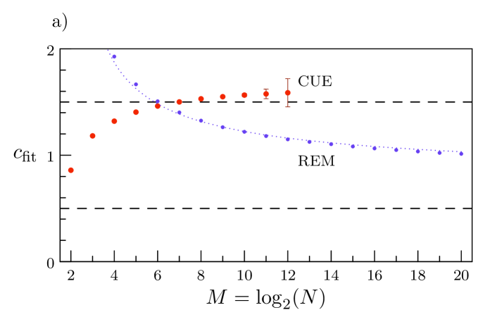
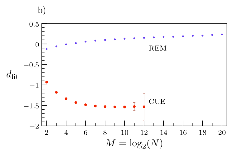
Note that $\log_{2}N=\log N/\log 2=M$ denotes the logarithm with base 2.
The error bars describe one standard deviation of the data (where no error bars are visible they are smaller than the dot size). The (blue) dotted curve in the upper panel is $0.5+1.4/\log\log N$ and shows that the REM data is consistent with $c_{\mathrm{fit}}=1/2+O\left(1/\log\log N\right)$. For the CUE data the deviations of $c_{\mathrm{fit}}$ from $c=3/2$ are consistent with a much faster decay (at least for the given range of matrix sizes $N$).

Figure 2: (Color online.) Integrated distribution function of $\log|p_{N}|_{\mathrm{max}}$ using the rescaled variable $x$ (see Eq. (18)) for REM (blue dashed curve for $N=1048576=2^{20}$) and CUE (red curve for $N=4096=2^{12}$) against the predicted curves.
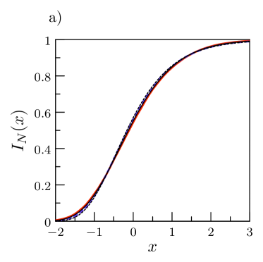
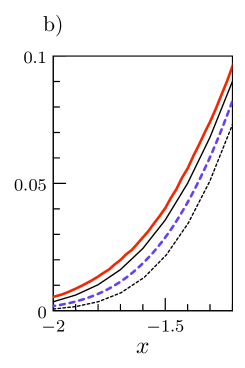
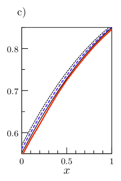
The full black line gives the CUE prediction. The dashed black line gives the Gumbel distribution (REM prediction). The left panel gives the whole distribution, the right two panels zoom into the distributions.

Figure 3: (Color online.) Difference between predicted integrated density distributions for $\log|p_{N}|_{\mathrm{max}}$ and numerically obtained distributions for various values of the size $N$ of the eigenvalue spectrum. The data is rescaled to vanishing mean and unit variance using the variable $x$ (see Eq. (18)).
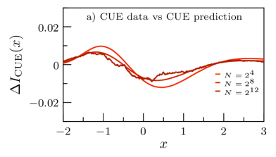
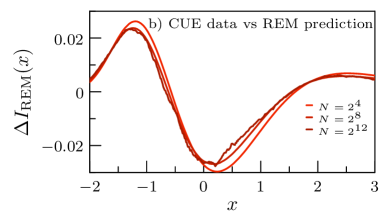
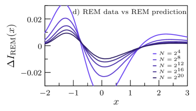
The left panels (a and b) show the difference between the two predictions and CUE data (for $N=2^{4}$, $2^{8}$, and $2^{12}$).
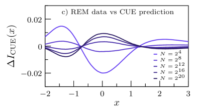
The right panels (c and d) show the difference between the two predictions and REM data (for $N=2^{4}$, $2^{8}$, $2^{12}$, $2^{16}$, and $2^{20}$).

In the case of the CUE, appropriate rescaling leads to an integrated distribution [18, 22, 23]

$$I_{\mathrm{CUE}}(y)=\int_{0}^{y}P_{\mathrm{CUE}}(y^{\prime})\ dy^{\prime}=2e^{-y/2}K_{1}(2e^{-y/2})$$ (13)

where $K_{1}(x)$ is the modified Bessel function of second kind and order one. The Gumbel and the CUE distributions are related by a simple convolution

$$P_{\mathrm{CUE}}(y)=\int_{-\infty}^{\infty}P_{\mathrm{Gumbel}}(y_{1})P_{\mathrm{Gumbel}}(y-y_{1})\ dy_{1}.$$ (14)

In other words if $y_{1}$ and $y_{2}$ are two independent Gumbel-distributed random numbers then their sum $y=y_{1}+y_{2}$ follows the CUE distribution. The scaling parameters obey

$$\begin{split}a_{N}=&-2\log N+c\log\log N+o(1)\\ b_{N}=&1+O(1/\log N)\end{split}$$ (15)

in both cases. The constant $c$ however takes different values

$$c=\begin{cases}\frac{1}{2}&\text{for $\mathrm{REM}$;}\\ \frac{3}{2}&\text{for $\mathrm{CUE}$.}\end{cases}$$ (16)

The different value of this constant is a key signature of the long range correlations in the CUE model. We tested this numerically by rescaling the data according to (11) using $a_{N}\equiv a_{\mathrm{fit}}$ and $b_{N}\equiv b_{\mathrm{fit}}$ as fitting parameters such that the rescaled data has the same mean and variance as the Gumbel distribution (for REM) or the CUE distribution (for CUE). From the fitted parameters we evaluated the quantities

$$\begin{split}c_{\mathrm{fit}}=&\frac{a_{\mathrm{fit}}+2\log{N}}{\log\log N}\ ,\\ d_{\mathrm{fit}}=&(b_{\mathrm{fit}}-1)\log N\ .\end{split}$$ (17)

From (15) we see that $c_{\mathrm{fit}}$ should converge to $c$ with corrections of order $o(1/\log\log N)$ while $d_{\mathrm{fit}}$ should be of order $O(1)$. In Fig. 1 we plot $c_{\mathrm{fit}}$ and $d_{\mathrm{fit}}$. The plots are consistent with the expected behaviour. Indeed, allowing deviations of order $O(1/\log\log N)$ the data is consistent with $c_{\mathrm{fit}}\to 3/2$ for CUE and $c_{\mathrm{fit}}\to 1/2$ for REM (the difference between $O(1/\log\log N)$ and $o(1/\log\log N)$ is too delicate to be resolved numerically).

Figure 4: (Color online.) Maximal difference of the three predicted integrated density distributions against the data for CUE and REM as a function of size $N$ of the eigenvalue spectrum. The one-sided error bars reflect the noise level – the upper dot is pure data without any smoothing the lower bar gives the difference for smoothed data (local average over an interval of size $0.5$).
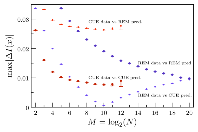
The thick (red) dots for $M=2$ to $M=12$ compare CUE data to the CUE prediction. The thin (red) dots for $M=2$ to $M=12$ compare the CUE data to the REM prediction. The thick (blue) dots for $M=2$ to $M=20$ compare REM data to the REM prediction. The thin (blue) dots for $M=2$ to $M=20$ compare REM data to the CUE prediction

A more detailed analysis of the distribution may be obtained by comparing the integrated distribution functions directly. For this we use the rescaled variable

$$x=\frac{\log|p_{N}|^{2}_{\mathrm{max}}-\mathbb{E}[\log|p_{N}|^{2}_{\mathrm{max}}]}{\sqrt{\mathrm{Var}[\log|p_{N}|^{2}_{\mathrm{max}}]}}$$ (18)

which has vanishing mean and unit variance. In Fig. 2 we plot the integrated distribution from the REM and CUE data against the predicted REM (Gumbel) and CUE distributions. The latter have been rescaled accordingly to have vanishing mean and unit variance and, with minor abuse of notation, we will write

$$I_{\mathrm{REM/CUE}}(x)\equiv I_{\mathrm{REM/CUE}}(y=\sqrt{\mathrm{Var}[y]}\ x+\mathbb{E}[y])\ .$$ (19)

One can see in Fig. 2 that the predicted curves and the curves obtained from numerical data are all very close to each other. Zooming into the details of the curves reveals that neither the REM curve has fully converged to the REM prediction (at $N=2^{20}$) nor has the CUE curve converged to the CUE prediction (at $N=2^{12}$).

We have analysed the convergence of the integrated distributions by considering the differences

$$\Delta I_{\mathrm{CUE/REM}}(x)=I_{N}(x)-I_{\mathrm{CUE/REM}}(x)$$ (20)

of the data ($I_{N}(x)$) for REM and CUE and the three predicted curves. In Fig. 3 we plot these differences for increasing values of the size $N$ of the eigenvalue spectrum. For REM the trend in these differences is clearly consistent only with the REM prediction. For CUE the picture is less clear because it was not feasible to diagonalise matrices larger than $N=2^{12}$. We ‘only’ diagonalised 50000 matrices of that size $N=2^{12}$ which gives much larger noise levels compared to smaller values of $N$ (at $N=2^{8}$ we diagonalised $10^{7}$ matrices). Nonetheless the numerics remains consistent with the CUE prediction.

A more detailed analysis of the convergence may be obtained by plotting the maximal difference $\mathrm{max}_{x\in\mathbb{R}}|\Delta I_{\mathrm{CUE/REM}}(x)|$ (i.e. the $L^{\infty}$-norm of the difference) against $N$, see Fig. 4. This confirms again that the REM data is consistent only with the REM prediction. For CUE the available data indicates that the difference to the REM prediction saturates at a finite value. The CUE data shows very slow convergence and the limited data at $N=2048$ and $N=4096$ results in a large error term – nonetheless the data is consistent with convergence of the CUE data to the conjectured prediction for CUE. Based on the data plotted in Fig. 4 one may estimate that one may require $N\times N$ matrices with $N=2^{20}$ or even larger in order to get a clearer support for the conjectured convergence. In order to get a sufficiently smooth integrated distribution function one has to fully diagonalise about $10^{6}$ to $10^{7}$ matrices. While there are specialised algorithms for sparse or banded matrices that obtain a fraction of the spectrum quite quickly we here need the full spectrum and computing the required amount of data is well beyond our limits.

We would like to mention that the extreme value distribution for characteristic polynomials of the Gaussian Unitary Ensemble GUE ensemble has also been discussed recently [25]. GUE spectra have the same logarithmic correlations as CUE spectra and the corresponding distribution of extreme values of characteristic polynomials shows similar deviations from the non-correlated REM spectra as CUE. The predicted curve $I_{\mathrm{GUE}}(x)$ is different but very close to the predicted curve $I_{\mathrm{CUE}}(x)$ (closer than to the REM curve $I_{\mathrm{REM}}(x)$). The origin of the difference is well understood – finite GUE spectra have Gaussian tails not present in CUE (see for [25] for further details). We have checked whether our CUE data is able to distinguish between the GUE and CUE predictions – however the two are too close to be resolved.

2.1 Correlations of the position of the maximal modulus of the characteristic polynomial and the spectrum

Figure 5: (Color online.) Integrated level spacing distributions $I_{\mathrm{ls}}(s;\theta_{\mathrm{max}})$ at $\theta_{\mathrm{max}}$ for CUE at $N=2^{8}=256$, $N=2^{10}=1024$ and $N=2^{12}=4096$.
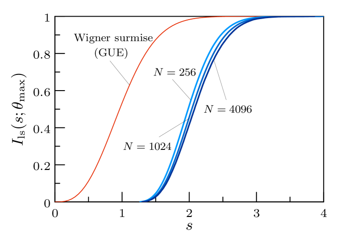
The thin (red) curve on the left is the integrated Wigner surmise for unitary ensembles. The three thick (blue) curves give the CUE data.

Figure 6: (Color online.) Integrated distribution $I_{\mathrm{fl}}(\tilde{\theta}_{\mathrm{max}})$ ($I_{\mathrm{fl}}(\tilde{\theta}_{\mathrm{min}})$) of the position $\tilde{\theta}_{\mathrm{max}}$ ($\tilde{\theta}_{\mathrm{min}}$) where the fluctuations of the spectral counting function are maximal (minimal) measured from the position of the maximum of the modulus of the characteristic polynomial (at $\tilde{\theta}=0$).

The spectrum $\{e^{i\phi_{n}}\}_{n=1}^{N}$ of the unitary matrix $U$ gives the zeros of the characteristic polynomial $|p_{N}(\theta)|$. One may expect that the position $\theta_{\mathrm{max}}$ where $|p_{N}(\theta_{\mathrm{max}})|=|p_{N}|_{\mathrm{max}}$ statistically occurs preferably in large intervals that are free of zeros. This kind of correlation may be measured in various ways. Most directly one may consider the level spacing distribution at $\theta=\theta_{\mathrm{max}}$. For any unitary matrix of dimension $N$ the mean level spacing over its complete spectrum is (trivially) $2\pi/N$. Numerically we find that typical values of level spacings at $\theta_{\mathrm{max}}$ for CUE matrices are about twice as large for the matrix sizes we used. This is a clear indication for correlation between the position $\theta_{\mathrm{max}}$ and large spacings for which we will give a more precise description in the following. Indeed our numerical analysis allows for a more detailed analysis of this deviation by considering the full statistical distribution of level spacings at $\theta_{\mathrm{max}}$ for CUE matrices. While it is very hard to make strong analytical predictions about the properties of this distribution (and we are not aware of any relevant results) it is numerically straightforward from the large amount of CUE spectra that we have computed. For each spectrum we have obtained the scaled levels spacing $s=N\left(\phi_{n+1}-\phi_{n}\right)/(2\pi)$ where $\phi_{n+1}>\theta_{\mathrm{max}}>\phi_{n}$. The integrated level spacing distribution $I_{\mathrm{ls}}(s;\theta_{\mathrm{max}})$ is then the ratio of the number of spectra where the rescaled level spacing is smaller than $s$ over the total number of spectra. In Fig. 5 we plot this quantity for $N=2^{8}$, $2^{10}$ and $2^{12}$ and compare it to the Wigner surmise. If $\theta_{\mathrm{max}}$ was a typical point in the spectrum one would expect to see a distribution close to the Wigner surmise and the expectation value of the level spacing would be close to unity. The plots in Fig. 5 show however strong deviations from the Wigner surmise and the expected level spacings are much larger than unity (and growing slowly with $N$). This is evidence for strong correlations between the position $\theta_{\mathrm{max}}$ of the maximum of the modulus of the characteristic polynomial and the spectrum close to this value.

From the correlations between the position $\theta_{\mathrm{max}}$ and the increased level spacings at this point one may expect further correlations between the maximal values of the characteristic polynomial and the spectrum. Let $\tilde{\theta}=\theta-\theta_{\mathrm{max}}\in[0,2\pi)$. The spectral counting function may be written as

$$N(\tilde{\theta})=\frac{N\tilde{\theta}}{2\pi}-\frac{1}{\pi}\mathrm{Im}\,\log\det(1-e^{i\theta_{\mathrm{max}}}U)+\frac{1}{\pi}\mathrm{Im}\,\log\det(1-e^{-i(\tilde{\theta}+\theta_{\mathrm{max}})}U)\ .$$ (21)

In this form it counts the number of states above $\theta_{\mathrm{max}}$ and it directly relates the spectrum of $U$ to the characteristic polynomial. The fluctuations in the spectral counting function

$$N_{\mathrm{fluct}}(\tilde{\theta})=\frac{1}{\pi}\mathrm{Im}\,\log\det(1-e^{-i(\tilde{\theta}+\theta_{\mathrm{max}})}U)$$ (22)

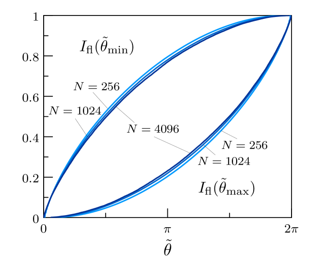
are expressed in terms of the argument of the characteristic polynomial $p_{N}(\theta)$. One may expect that the position of the maximum is correlated with large fluctuations. Numerically we obtain the values $\tilde{\theta}_{\mathrm{max}}$ and $\tilde{\theta}_{\mathrm{min}}$ where $N_{\mathrm{fluct}}(\tilde{\theta})$ takes its maximal and minimal values. In Fig. 6 we plot the integrated density $I_{\mathrm{fl}}(\tilde{\theta})$ of these values as a function of $\tilde{\theta}$. In absence of correlations one expects a straight line $\tilde{\theta}/(2\pi)$. However, the plots show deviations from a straight line that imply strong correlations between the position of the maximum of the modulus of the characteristic polynomial and the positions of the extrema in the fluctuations of the spectral counting function. The plots are consistent with the previous observation of large level spacings at $\tilde{\theta}=0$. At the beginning (end) of a large level spacings one may expect that $N_{\mathrm{fluct}}(\tilde{\theta})$ has a statistical tendency to be positive (negative). At $\tilde{\theta}=0$ we have found exceptionally large spacings and thus may expect a statistical correlation that a maximal positive fluctuation occurs before and that a maximal negative fluctuation (i.e. its minimum) occurs just above $\tilde{\theta}=0$. This is clearly shown in the plotted integrated densities. In addition these plots show that these correlations are long ranged and certainly do not decay on the scale of the mean level spacing $2\pi/N$ (the scale for spectral $n$-point correlation functions in CUE).

The correlations we have found numerically point to interesting effects that are currently not understood on a theoretical level. Analytical approaches to these kinds of correlations would be highly desirable.

3 The free energy and its distribution

Figure 7: (Color online.) Expectation value of the free energy as function of the inverse temperature $\beta$. Upper panel: the thick (red) lines give CUE data for $N=2^{6}$ and $N=2^{12}$ the thin (black) line is the theoretical predicition for $N\to\infty$. Lower panel: the thick (blue) lines give REM data for $N=2^{6}$, $N=2^{12}$ and $N=2^{18}$ and the thin (black) line is the theoretical predicition for $N\to\infty$.
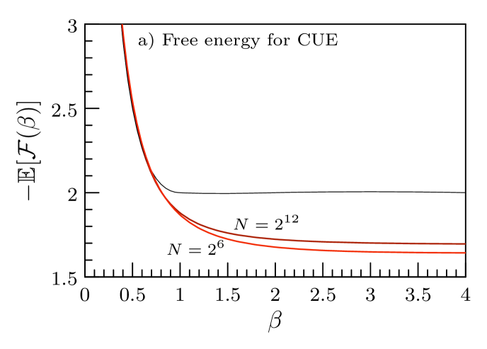
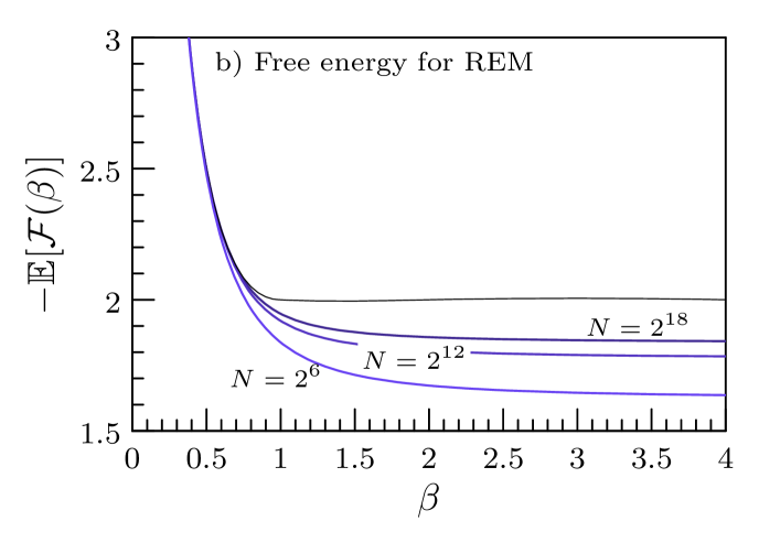
Note that the scale for the ordinate starts at the value $1.5$.

Figure 8: (Color online.) Convergence of the expected free energy at $\beta=3$. The plot shows the difference of the expected value $-\mathbb{E}[\mathcal{F}(3)]=2$ and the data for CUE (thick red dots) and REM (thin blue dots), rescaled by a factor $\log N/\log(\log N)$. The two thin dotted lines correspond to fitted curves of the form (23) (see main text for explanation).

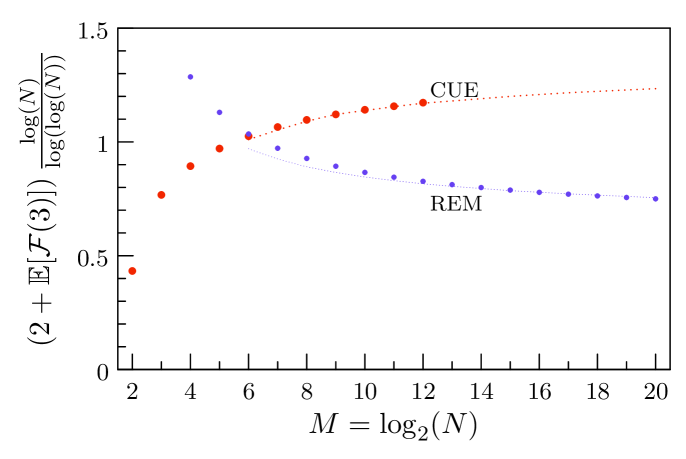
In Sec. 1.1 we introduced the partition sum $\mathcal{Z}_{N}(\beta)$ and the free energy $\mathcal{F}_{N}(\beta)$ for CUE and REM. Numerically they are straightforwardly obtained from the eigenvalue spectra that we have obtained for both models (by numerical integration over the spectral angle $\theta$).

In Fig. 7 we plot the expected free energy $\mathbb{E}[\mathcal{F}_{N}(\beta)]$ as a function of the inverse temperature $\beta$ for CUE and REM and some values of $N$. In both cases we see freezing but the convergence to the predicted curve for $N\to\infty$ above the freezing transition $\beta\geq 1$ is quite slow. In the freezing regime the free energy is dominated by the maximal value of the modulus of the characteristic polynomial. In the previous section we have confirmed the prediction that the latter obey $2\log|p_{N}|_{\mathrm{max}}^{2}\sim 2\log N-c\log\log N+o(1)$ where $c=3/2$ for CUE and $c=1/2$ for REM (see (16)). For the free energy this implies convergence at a slow rate $\log\log N/\log N$ in the freezing regime. We test this estimate numerically by considering the difference of the numerically obtained free energy at $\beta=3$ to the theoretical value $\mathbb{E}[\mathcal{F}(3)]=-2$. We compare this to a fitted curve of the form

$$-\mathcal{F}_{\mathrm{fit}}=2-c\frac{\log\log N}{\log N}+\frac{g_{\mathrm{fit}}}{\log N}$$ (23)

where the additional parameter $g_{\mathrm{fit}}$ is fitted to the data at $N=2^{12}$ for CUE where $g_{\mathrm{fit}}\approx 0.69$ and at $N=2^{20}$ for REM where $g_{\mathrm{fit}}\approx-0.67$. In Fig. 8 we plot the difference of the conjectured expectation value $-\mathbb{E}[\mathcal{F}(3)]\to 2$ for $N\to\infty$ and the numerical expectation value at finite values of $N$. In the plots we have rescaled the difference by a factor $\log N/\log(\log N)$). For both models the plots are consistent with a saturation at the value $c=3/2$ or $c=1/2$ for CUE and REM with higher order deviations $\approx\frac{g_{\mathrm{fit}}}{\log\log N}$.

Figure 9: (Color online.) Integrated distribution of the rescaled partition function for inverse temperatures below the freezing transition at $\beta=0.5$ (red curves) and $\beta=0.8$ (orange curves). We plot the curves as a function of $z^{1/\beta^{2}}$ where $z$ is the appropriately rescaled partition function (see Eq. (24)). This makes the predicted limiting distribution independent of $\beta$. The different plots are for $N=16$, $64$, $256$, $1024$, and $4096$ (with increasing strength of color). The dashed black curve is the predicted curve for $N\to\infty$.

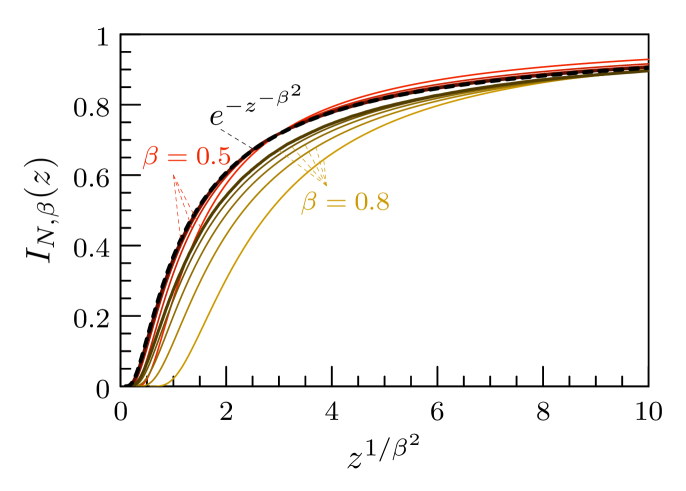
Next we consider the distribution of the partition function $\mathcal{Z}_{N}(\beta)$ for the CUE model (we do not show that data for the well-understood REM model, because it does not give additional insight to what we have learned from the comparison so far). For inverse temperatures below the freezing transition $\beta<1$ an analytical prediction is available for the complete distribution. For this purpose one rescales the partition function

$$z=\mathcal{Z}_{N}(\beta)/\mathcal{Z}_{e}(\beta)$$ (24)

where $\mathcal{Z}_{e}(\beta)=N^{1+\beta^{2}}\frac{G^{2}(1+\beta)}{G(1+2\beta)G(1-\beta^{2})}$ and $G(x)$ is the Barnes $G$-function. In the limit $N\to\infty$ the prediction for the integrated probability distribution of the rescaled partition function is

$$I_{\beta}(z)=e^{-z^{-1/\beta^{2}}}\ .$$ (25)

In Fig. 9 we plot the numerically obtained integrated distribution function $I_{N,\beta}(z)$ for CUE for $\beta=0.5$ and $\beta=0.8$. For $\beta=0.5$ one sees clear and quick convergence to the predicted curve. For $\beta=0.8$, somewhat closer to the freezing transition, convergence is slower but consistent with the prediction.

In the freezing regime $\beta>1$ a theoretical prediction for the distribution as $N\to\infty$ of the partition function is known only in the form of a Laplace transform (see eq (33) in [18]) to the leading order

$$\int_{0}^{\infty}I_{N,\beta}(Z)e^{-sZ}dZ=2\nu s^{\frac{1}{2\beta}-1}K_{1}(2\nu s^{\frac{1}{2\beta}})\ .$$ (26)

Here the parameter

$$\nu=\frac{N^{2}}{\log^{3/2}N}\nu_{\mathrm{red}}$$ (27)

sets the overall scale and $\nu_{\mathrm{red}}$ (the reduced parameter) is of order $O(1)$. This implies that the appropriately rescaled partition function

$$\tilde{z}=\mathcal{Z}_{N}(\beta)\frac{\log^{3\beta/2}N}{N^{2\beta}}$$ (28)

has a finite limiting distribution $I_{\beta}(\tilde{z})$. The Laplace transform of the latter is obtained from (26) by replacing $\nu\mapsto\nu_{\mathrm{red}}$, i.e. $\int_{0}^{\infty}I_{\beta}(\tilde{z})e^{-s\tilde{z}}d\tilde{z}=2\nu_{\mathrm{red}}s^{\frac{1}{2\beta}-1}K_{1}(2\nu_{\mathrm{red}}s^{\frac{1}{2\beta}})$. The value of the scale $\nu_{\mathrm{red}}$ is not known theoretically and it is not straightforward to extract numerically from data at finite $N$ because of the generally slow convergence of the model and the fact that the distribution at finite $N$ depends not only on the scale factor $\nu$ but also on the shape, which is currently not known theoretically. As a practical way to obtain a value for $\nu_{\mathrm{red}}$ we consider the theoretical expectation value of $\log\tilde{z}$ as a function of $\beta$ and $\nu_{\mathrm{red}}$. Numerically the simple scaling implies that one can extract the full dependence of $\mathbb{E}[\log\tilde{z}]$ on the parameter $\nu_{\mathrm{red}}$ for any given value of $\beta$ by obtaining the inverse Laplace transform at $\nu_{\mathrm{red}}=1$. At $\beta=3$ the scaling just gives

$$\mathbb{E}[\log\tilde{z}]\approx 6\log(\nu_{\mathrm{red}})+0.87.$$ (29)

We compare this to the numerical fit (23) to the data for the free energy shown in Fig. 8 at the same value $\beta=3$

$$\mathbb{E}[\log\tilde{z}]=3g_{\mathrm{fit}}\approx 2.07$$ (30)

where the factor $3$ on the right hand side is $\beta$. This results in an approximate value $\nu_{\mathrm{red}}\approx e^{0.2}\approx 1.22$. We do not claim that our practical approach gives the correct value as $N\to\infty$. We will use this scale for comparing the integrated distributions of $\tilde{z}$.

In Fig. 10 we plot the numerically obtained integrated distributions $I_{N,\beta}(\tilde{z})$ of $\tilde{z}$ at the critical point ($\beta=1$) and in the freezing regime ($\beta=2$ and $\beta=3$). The curves in the freezing regime are consistent with the existence of a limiting distribution on this scale though the convergence to the predicted limiting distribution may be very slow. Note that the predicted curves contain one fitting parameter $\nu_{\mathrm{red}}$. In Fig. 10 we have used the value $\nu_{\mathrm{red}}=1.22$ obtained from the procedure outlined above. Setting $\nu_{\mathrm{red}}=1$ leads to a limiting curve where the ordinate is stretched by a factor $\nu_{\mathrm{red}}^{2}\approx 1.5$. While this looks much closer to the data at the finite values of $N$ we should reiterate that no theoretical predictions about the leading corrections of the shape of this curve are available and one should expect these deviations to decay slowly (e.g. as $1/\log N$ or even slower). Furthermore note that our numerics indicates that at the critical temperature $\beta=1$ the scaling (28) is no longer valid. This is consistent with the prediction that a different power of $\log N$ is expected at the transition point (see eq.(45b) of [9]).

Figure 10: (Color online.) Integrated distribution of the rescaled partition function for inverse temperatures at the critical value $\beta=1$ (green curves) of the freezing transition and in the freezing regime at $\beta=2$ (orange curves) and $\beta=3$ (red curves). We plot the curves as a function of $\tilde{z}^{1/\beta}$ where $\tilde{z}$ is the appropriately rescaled partition function (see Eq. (28)). The different plots are for $N=256$, $1024$, and $4096$ (with increasing strength of color). The dashed lines give the theoretical prediction given by (26) where the overall scale parameter $\nu_{\mathrm{red}}$ has been fitted by the procedure outlined in the main text.

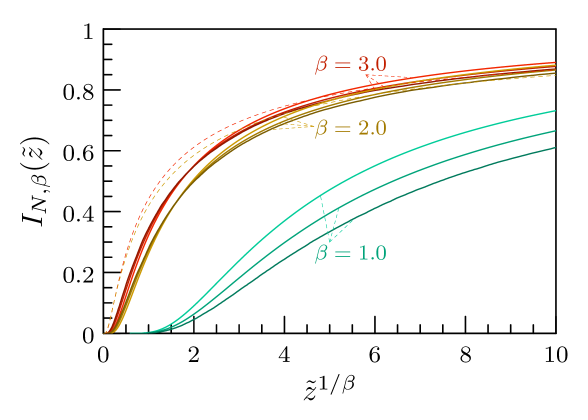
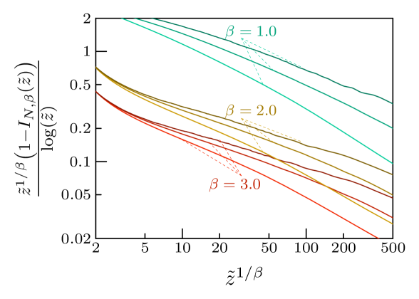
From (26) one may deduce that the tails (at large values of the partition function) behave like

$$1-I_{\beta}(\tilde{z})\propto\tilde{z}^{-1/\beta}\log\tilde{z}$$ (31)

where the logarithm is related to the strong correlation in CUE. In Fig. 11 we plot the ratio of the numerically obtained tails $1-I_{N,\beta}(\tilde{z})$ and the predicted behaviour for $\beta>1$. In order to confirm the prediction one should see the appearance of a saturation at a finite value as $\tilde{z}$ increases. While the available numerical data at finite $N$ cannot confirm this prediction the numerics is consistent with the appearance of such a saturation as $N\to\infty$. Indeed the curves for $\beta=2$ and $\beta=3$ indicate that the behaviour in the tails for finite $N$ may be of the form $1-I_{\beta}(\tilde{z})\propto\tilde{z}^{-1/\beta-\nu_{\beta}(N)}\log\tilde{z}$ where the additional exponent $\nu_{\beta}(N)>0$ decays to zero as $N\to\infty$.

Figure 11: (Color online.) Tail of the integrated distribution of the rescaled partition function at the critical inverse temperature $\beta=1$ (green curves) and in the freezing regime at $\beta=2$ (orange curves) and $\beta=3$ (red curves). The tail $1-I_{N,\beta}(\tilde{z})$ is divided by $\tilde{z}^{-1/\beta}\log\tilde{z}$ according to the predicted behaviour in the freezing regime. The different plots are for $N=256$, $1024$, and $4096$ (with increasing strength of colour).

4 Conclusions and Outlook

The numerical results we have presented here are consistent with the conjectures put forward in [22, 23]. Taken together with recent proofs of some of these conjectures, there is growing evidence supporting the underlying philosophy that the characteristic polynomials of random matrices behave statistically like logarithmically-correlated Gaussian fields. However, the convergence to the limiting formulae predicted is clearly very slow, and much more extensive numerical experiments will be required in order to examine the details of the various conjectures. The rates of convergence we have found in our computations are suggestive. It would be extremely interesting if they could be verified by a more refined asymptotic analysis than that carried out in [22, 23].

We believe the correlations we have found between the extreme values of characteristic polynomials and eigenvalue spacings to be interesting and worthy of theoretical study. There has for some time been a folklore belief that these correlations should exist, but as far as we understand ours is the first quantitative study of them. It may be possible to analyse these by extending the heuristic asymptotic analysis of [22, 23] to mixed moments involving both the modulus and the argument of the characteristic polynomial (as in the moment calculations of [29]). It should also be possible to do a similar quantitative analysis for the Riemann zeta-function, where extensive data exist.

It should be clear that the computations we have described here are first steps in what we believe may be a worthwhile new line of research. We hope that that they will inspire further numerical studies as well as new theory.

5 Appendix A: Moments of the partition function

Let

$$M_{N,\beta,k}=\mathbb{E}\left[\mathcal{Z}_{N}(\beta)^{k}\right]\$$ (32)

be the $k$-th moment of the partition function. A conjecture in [22, 23] states $M_{N,\beta,k}\sim N^{1+\beta^{2}k^{2}}$. If $\beta$ and $k$ are positive integers one may calculate these moments directly for arbitrary matrix dimension from the autocorrelation function of order $k$ for the characteristic polynomials [5]. It is striking that exact formulae can be written down for this quantity, especially at the point of the freezing transition. As a benchmark for our numerics we compare some low moments with the analytically known values. Analytically one finds [5]

$$M_{N,1,1}= (N+1)N = N^{2}M_{N,1,1}^{\mathrm{red}}$$

$$M_{N,1,2}= N^{2}\binom{N+3}{3} = \frac{N^{5}}{6}M_{N,1,2}^{\mathrm{red}}$$

$$M_{N,1,3}= \frac{N^{3}(N+5)!}{2520N!}(N^{2}+6N+21) = \frac{N^{10}}{2520}M_{N,1,3}^{\mathrm{red}}$$

$$M_{N,1,4}= \frac{8N^{4}(N+7)!}{13!N!}\left(7N^{6}+168N^{5}+1804N^{4}\right.$$

$$\left.\qquad+10944N^{3}+41893N^{2}+99624N+154440\right) = \frac{56N^{17}}{13!}M_{N,1,4}^{\mathrm{red}}$$

$$M_{N,2,1}= \frac{(N+2)(N+3)!}{12(N-1)!} = \frac{N^{5}}{12}M_{N,2,1}^{\mathrm{red}}$$

$$M_{N,2,2}= \frac{8N^{2}(N+7)!}{15!N!}\left(298N^{8}+9536N^{7}+134071N^{6}\right.$$

$$\qquad+1081640N^{5}+549437N^{4}+18102224N^{3}$$

$$\left.\qquad+38466354N^{2}+50225040N+32432400\right) = \frac{2384N^{17}}{15!}M_{N,2,2}^{\mathrm{red}}.$$

We have here introduced as well the reduced moments $M^{\mathrm{red}}_{N,\beta,k}$. The reduced moments obey $M^{\mathrm{red}}_{N,\beta,k}\to 1$ as $N\to\infty$ and are of order unity for finite values of $N$. The following tables compare the known exact values of the reduced moments $M^{\mathrm{red}}_{N,\beta,k}$ with the corresponding reduced moments $\overline{\mathcal{Z}_{N}(\beta)^{k}}^{\mathrm{\ red}}$ obtained from the numerical data. In each case the given errors are one statistical standard deviation. We only present data that has sufficiently converged (i.e the standard deviation is sufficiently small). The statistical errors are consistent with the scaling with $N$ of the prediction for higher moments (which determine standard deviations) $\propto N^{\beta^{2}k^{2}-1/2}$.

$N$	$M^{\mathrm{red}}_{N,1,1}$	$\overline{\mathcal{Z}_{N}(1)}^{\mathrm{\ red}}$
$4$	$1.25$	$1.25031\pm 0.00013$
$8$	$1.125$	$1.12505\pm 0.00018$
$16$	$1.0625$	$1.06230\pm 0.00026$
$32$	$1.03125$	$1.03145\pm 0.00036$
$64$	$1.01562\dots$	$1.01682\pm 0.00078$
$128$	$1.0078\dots$	$1.0076\pm 0.0013$
$256$	$1.0039\dots$	$1.0056\pm 0.0023$
$512$	$1.0019\dots$	$1.0014\pm 0.0019$
$1024$	$1.0009\dots$	$0.9959\pm 0.0046$
$2048$	$1.0004\dots$	$1.011\pm 0.014$
$4096$	$1.0002\dots$	$0.998\pm 0.055$

$N$	$M^{\mathrm{red}}_{N,1,2}$	$\overline{\mathcal{Z}_{N}(1)^{2}}^{\mathrm{\ red}}$
$4$	$3.2812\dots$	$3.2835\pm 0.0010$
$8$	$1.9335\dots$	$1.9352\pm 0.0018$
$16$	$1.4194\dots$	$1.4158\pm 0.0054$
$32$	$1.198\dots$	$1.170\pm 0.012$
$64$	$1.096\dots$	$1.241\pm 0.135$
$128$	$1.047\dots$	$0.856\pm 0.050$
$256$	$1.023\dots$	$1.238\pm 0.352$
$512$	$1.011\dots$	$0.456\pm 0.029$
$1024$	$1.005\dots$	$0.49\pm 0.17$

$N$	$M^{\mathrm{red}}_{N,1,3}$	$\overline{\mathcal{Z}_{N}(1)^{3}}^{\mathrm{\ red}}$
$4$	$56.293\dots$	$56.362\pm 0.039$
$8$	$9.794\dots$	$9.850\pm 0.058$
$16$	$3.39\dots$	$3.28\pm 0.14$
$32$	$1.88\dots$	$1.19\pm 0.10$
$64$	$1.38\dots$	$1.74\pm 0.98$

$N$	$M^{\mathrm{red}}_{N,1,4}$	$\overline{\mathcal{Z}_{N}(1)^{4}}^{\mathrm{\ red}}$
$4$	$9156.3\dots$	$9171.0\pm 12.4$
$8$	$201.9\dots$	$206.1\pm 5.2$
$16$	$18.38\dots$	$1.36\pm 0.21$

$N$	$M^{\mathrm{red}}_{N,2,1}$	$\overline{\mathcal{Z}_{N}(2)}^{\mathrm{\ red}}$
$4$	$4.9218\dots$	$4.9255\pm 0.0015$
$8$	$2.4169\dots$	$2.4190\pm 0.0023$
$16$	$1.5968\dots$	$1.5926\pm 0.0061$
$32$	$1.273\dots$	$1.243\pm 0.013$
$64$	$1.130\dots$	$1.289\pm 0.147$
$128$	$1.063\dots$	$0.869\pm 0.056$
$256$	$1.03\dots$	$1.21\pm 0.36$

$N$	$M^{\mathrm{red}}_{N,2,2}$	$\overline{\mathcal{Z}_{N}(2)^{2}}^{\mathrm{\ red}}$
$4$	$27270.2\dots$	$27313.8\pm 32.9$
$8$	$402.9\dots$	$409.7\pm 8.4$
$16$	$27.57\dots$	$21.4\pm 2.9$
$32$	$5.79\dots$	$0.78\pm 0.18$

6 Appendix B: On the maximum of characteristic polynomial for $\beta-$circular ensemble.

Consider the circular $\beta-$ ensemble with j.p.d. of real variables $\theta_{i}\in[0,2\pi),\,i=1,\ldots,N$ given by [30]

$${\cal P}_{\beta}(\theta_{1},\ldots,\theta_{N})=\frac{1}{(2\pi)^{N}C_{N,\beta}}\prod_{i<j}^{N}|e^{i\theta_{i}}-e^{i\theta_{j}}|^{\beta},\quad C_{N,\beta}=\frac{\Gamma\left(1+N\beta/2\right)}{\Gamma^{n}(1+\beta/2)},\quad\beta>0$$ (33)

and denote $\left\langle\ldots\right\rangle_{C\beta E_{N}}$ the corresponding averages. Further introduce the characteristic polynomial $p_{N}(\theta)=\prod_{i}^{N}\left(1-e^{i(\theta_{i}-\theta)}\right)$ by Eq.(2) in terms of which we define the partition function

$$\mathcal{Z}_{q}=\frac{N}{2\pi}\int_{0}^{2\pi}|p_{N}(\theta)|^{2q}\,d\theta,\quad q>0$$ (34)

where $q$ is the inverse temperature (we can not use $\beta$ here for the inverse temperature as that is reserved for the Dyson index). Integer moments of the partition function are then given by

$$\mathbb{E}\left\{\mathcal{Z}_{q}^{n}\right\}=\frac{N^{n}}{(2\pi)^{n}}\int_{0}^{2\pi}\ldots\int_{0}^{2\pi}\mathbb{E}\left\{\prod_{l=1}^{n}|p_{N}(\theta_{l})|^{2q}\right\}\,d\theta_{1}\ldots d\theta_{n}$$ (35)

where

$$\mathbb{E}\left\{\prod_{l=1}^{n}|p_{N}(\theta_{l})|^{2q}\right\}=\frac{1}{(2\pi)^{N}C_{N,\beta}}\int\prod_{i<j}^{N}\,|e^{i\theta_{i}}-e^{i\theta_{j}}|^{\beta}\prod_{i=1}^{N}g(\theta_{i})\,d\theta_{i}\equiv\left\langle\prod_{i=1}^{N}g(\theta_{i})\right\rangle_{C\beta E_{N}}$$ (36)

and we defined the “symbol” function

$$g(\theta)=\prod_{l=1}^{n}\left(2-2\cos{\left(\theta_{l}-\theta\right)}\right)^{q}$$ (37)

which can be rewritten as

$$\log{g(\theta)}=\sum_{l=1}^{n}\,q\log\left(2-2\cos{\left(\theta_{l}-\theta\right)}\right).$$ (38)

The last equation when compared to Eq.(1.6) from [16] implies

$$a(\theta)=1,\quad a_{l}=q,\,b_{l}=0\quad\forall l=1,\ldots,n,$$ (39)

If the parameter $\beta$ is rational ( that is: $\beta=2s/r$ where $s$ and $r$ are relatively prime) the paper [16] conjectured the generalisation of Fisher-Hartwig formula for $N\to\infty$, which in the case of (39) reads (see (3.13)-(3.14) in [16] with identification $R=n$ and $q_{j}=2q/\beta,\,\forall j)$ as well as $c_{n}=0,\,\forall n$):

$$\left\langle\prod_{i=1}^{N}g(\theta_{i})\right\rangle_{C\beta E_{N},\,N\to\infty}\sim N^{\frac{2nq^{2}}{\beta}}A^{n}|_{\left(q_{j}=2q/\beta\right)}\prod_{l<m}^{n}\left|e^{i\theta_{l}}-e^{i\theta_{m}}\right|^{-\frac{4q^{2}}{\beta}}$$ (40)

and the function $A|_{q_{j}}$ is given by a complicated product of Barnes functions in eq.(3.11) of [16]. Substituting the above to (35) and defining $\tilde{q}=q\sqrt{\frac{2}{\beta}}$ we get:

$$\mathbb{E}\left\{\mathcal{Z}_{q}^{n}\right\}=N^{\frac{2nq^{2}}{\beta}}A^{n}|_{\left(q_{j}=2q/\beta\right)}\frac{N^{n}}{(2\pi)^{n}}\int_{0}^{2\pi}\ldots\int_{0}^{2\pi}\,\prod_{l<m}^{n}\left|e^{i\theta_{l}}-e^{i\theta_{m}}\right|^{-2\tilde{q}^{2}}\,d\theta_{1}\ldots d\theta_{n}$$ (41)

$$=\mathcal{Z}^{n}_{e}(\tilde{q})\Gamma(1-n\tilde{q}^{2})$$ (42)

where we introduced the “typical value” for the partition function

$$\mathcal{Z}_{e}(\tilde{q})=N^{1+\tilde{q}^{2}}A|_{\left(q_{j}=2q/\beta\right)}\frac{1}{\Gamma(1-\tilde{q}^{2})}$$ (43)

We see that the “freezing temperature” is now given by the condition $\tilde{q}=1$ so that $q=\sqrt{\frac{\beta}{2}}$. The “free energy” is given by, to the leading order for $N\to\infty$:

$$-{\cal F}=\frac{1}{q\log{N}}\log{\mathcal{Z}_{q}}\to\left\{\begin{array}[]{cc}\frac{1}{q}+\frac{2}{\beta}q,&q<\sqrt{\frac{\beta}{2}}\\ 2\sqrt{\frac{2}{\beta}},&q>\sqrt{\frac{\beta}{2}}\end{array}\right.$$ (44)

Correspondingly, the leading order of the maximum of the characteristic polynomial is given by $\sqrt{\frac{2}{\beta}}\log{N}$. To find the subleading order one can follow the same procedure as for $\beta=2$ and find that the typical measure of “high points” , that is those points where $2\log{|p_{n}(\theta)|}>2x\log{N}$ is given by

$$\mu_{e}(x)\sim\frac{N^{-\beta x^{2}/2}}{\log N}\frac{1}{\Gamma\left(1-\beta x^{2}/2\right)}$$ (45)

and equating this to $N^{-1}$ we find the ”threshold of high values” to be

$$x=\sqrt{\frac{2}{\beta}}\left(1-\frac{3}{4}\frac{\log{\log{N}}}{\log{N}}\right)$$ (46)

which implies two first terms of the maximum to be $\sqrt{\frac{2}{\beta}}\left(\log{N}-\frac{3}{4}\log{\log{N}}\right)$, in full agreement with [11]. Finally, the correction term of the order of unity will be obviously given by the same distribution as for $\beta=2$, as moments of the partition function are the same, up to a trivial rescaling by $\sqrt{\frac{2}{\beta}}$ whenever necessary.

We therefore come to the conclusion that as $N\to\infty$ the characteristic polynomials of circular ensemble for any $\beta>0$ is essentially described by the same random Gaussian logarithmically correlated process rescaled by the parameter $\sqrt{\frac{2}{\beta}}$.

References

- [1] L.-P. Arguin, D. Belius, and A. J. Harper. Maxima of a randomised Riemann zeta function, and branching random walks. Ann. Appl. Probab. 27, 178-215 (2017)
- [2] L.-P. Arguin, D. Belius, and P. Bourgade. Maximum of the characteristic polynomial of random unitary matrices. Comm. Math. Phys. 349, 703-751 (2017)
- [3] L.-P. Arguin, D. Belius, P. Bourgade, M.Radziwiłł and K. Soundararajan. Maximum of the Riemann zeta function on a short interval. Commun. Pure & Appl. Math. in print (2018) ( arXiv:1612.08575[math.PR])
- [4] K. Astala, P. Jones, A. Kupiainen, and E. Saksman: Random conformal weldings. Acta Math. 207, 203–254 (2011)
- [5] E. Bailey and J.P. Keating. On the moments of the moments of the characteristic polynomials of random unitary matrices. arXiv:1807.06605[math-ph] (2018)
- [6] N. Berestycki.An elementary approach to Gaussian multiplicative chaos. Electron. Commun. Probab. 22, 1-12 (2017)
- [7] N. Berestycki, C. Webb, and M. D. Wong. Random Hermitian matrices and Gaussian multiplicative chaos. Probab. Theory and Rel. Fields 172, 103-189 (2018)
- [8] J-P Bouchaud and M. Mezard. Universality Classes for Extreme Value Statistics. J. Phys. A: Math. Gen. 30, 7997-8015 (1997)
- [9] D. Carpentier and P. Le Doussal. Glass transition of a particle in a random potential, front selection in nonlinear renormalization group, and entropic phenomena in Liouville and sinh-Gordon models.Phys. Rev. E 63, 026110 (2001)
- [10] C. Chamon, C. Mudry, X-G. Wen. Localization in two dimensions, gaussian field theories, and multifractality. Phys. Rev. Lett. 77, 4194-4198 (1996)
- [11] R Chhaibi, T Madaule, J Najnudel. On the maximum of the CE field. Duke Math. J. 167, 2243-2345 (2018)
- [12] B. Derrida. Random energy model: an exactly solvable model of disordered systems. Phys. Rev. B 24, 2613-2626 (1981).
- [13] B. Derrida, H. Spohn. Polymers on disordered trees, spin glasses, and travelling waves. J Stat Phys 51, 817-840 (1988)
- [14] J. Ding, R. Roy, and O. Zeitouni. Convergence of the centered maximum of log-correlated Gaussian fields. Ann. Probab. 45, 3886-3928 (2017)
- [15] I. Dumitriu, A. Edelman. Matrix models for beta ensembles. J. Math. Phys. 43, 5830-5847 (2002)
- [16] P.J. Forrester and N.E. Frankel. Applications and generalizations of fisher-Hartwig asymptotics. J. Math. Phys. 45, 2003-2028 (1994)
- [17] Y.V. Fyodorov. Multifractality and freezing phenomena in random energy landscapes: An introduction. Physica A 389 4229-4254 (2010)
- [18] Y.V. Fyodorov and J.-P. Bouchaud. Freezing and extreme-value statistics in a random energy model with logarithmically correlated potential. J. Phys. A: Math. Theor. 41 372001 (2008)
- [19] Y.V. Fyodorov, P. Le Doussal, and A. Rosso. Statistical mechanics of logarithmic REM: duality, freezing and extreme value statistics of noises generated by Gaussian free fields. J. Stat. Mech. 2009, P10005 (2009)
- [20] YV Fyodorov, P Le Doussal, A Rosso. Counting function fluctuations and extreme value threshold in multifractal patterns: the case study of an ideal 1/f noise. J. Stat. Phys. 149, 898-920 (2012)
- [21] Y.V. Fyodorov and P. Le Doussal. Moments of the position of the maximum for GUE characteristic polynomials and for log-correlated Gaussian processes J. Stat. Phys. 164, 190-240 (2016)
- [22] Y.V. Fyodorov, G.A. Hiary, and J.P. Keating. Freezing transitions, characteristic polynomials of random matrices, and the Riemann zeta-function. Phys. Rev. Lett. 108, 170601 (2012).
- [23] Y.V. Fyodorov and J.P. Keating. Freezing transitions and extreme values: random-matrix theory, and disordered landscapes. Phil. Trans. Roy. Soc. A 372, 20120503 (2014)
- [24] Y. V. Fyodorov, B. A. Khoruzhenko, and N. J. Simm. Fractional Brownian motion with Hurst index and the Gaussian Unitary Ensemble. Ann. Probab. 44, 2980-3031 (2016)
- [25] Y V Fyodorov and N J Simm. On the distribution of the maximum value of the characteristic polynomial of GUE random matrices. Nonlinearity 29, 2837-2855 (2016)
- [26] C.P. Hughes, J.P. Keating and N O’Connell. On the characteristic polynomial of a random unitary matrix. Commun. Math. Phys. 220, 429-451 (2001)
- [27] J.-P. Kahane. Sur le chaos multiplicatif. Ann. Sci. Math. Québec. 9, 105-150 (1985)
- [28] J.P. Keating. Random matrices and number theory: some recent themes. in: Stochastic Processes and Random Matrices: Lecture Notes of Les Houches Summer School: July 2015. Session CIV. Ed. by G. Schehr et al. (Oxford University Press, 2017)
- [29] J.P. Keating and N.C. Snaith. Random matrix theory and , Commun. Math. Phys. 214, 57-89 (2000)
- [30] R. Killip and I. Nenciu. Matrix Models for Circular Ensembles Int. Mathematical Research Notices 2004, 2665-2701 (2004)
- [31] J. Najnudel. On the extreme values of the Riemann zeta function on random intervals of the critical line. Probab. Theory Relat. Fields 172 387-452 (2018)
- [32] A. Kupiainen, R. Rhodes, V. Vargas. The DOZZ formula from the path integral] JHEP May 2018:94 (2018)
- [33] B. B. Mandelbrot, Possible refinement of the log-normal hypothesis concerning the distribution of energy dissipation in intermittent turbulence, in Statistical Models and Turbulence. M. Rosenblatt and C. Van Atta, eds., Lecture Notes in Physics 12, (Springer, New York, 1972), p. 333.
- [34] D. Ostrovsky. On Barnes beta distributions and applications to the maximum distribution of the 2D Gaussian Free Field. J. Stat. Phys. 164, 1292-1317 (2016)
- [35] D. Ostrovsky. A review of conjectured laws of total mass of Bacry–Muzy GMC measures on the interval and circle and their applications. Rev. Math. Phys. 30, 1830003 (2018)
- [36] E. Paquette O. Zeitouni. The Maximum of the CUE Field. Int. Math. Res. Notices 2018, 5028-5119 (2018)
- [37] E.Saksman, C. Webb. The Riemann zeta function and Gaussian Multiplicative Chaos: statistics on the critical line. arXiv:1609.00027[math.PR] (2016)
- [38] E. Subag, O. Zeitouni. Freezing and decorated Poisson point processes. Commun. Math. Phys. 337, 55-92 (2015)
- [39] R. Rhodes, V. Vincent. Lecture notes on Gaussian multiplicative chaos and Liouville Quantum Gravity. in: Stochastic Processes and Random Matrices: Lecture Notes of Les Houches Summer School: July 2015. Session CIV. Ed. by G. Schehr et al. (Oxford University Press, 2017)
- [40] G. Remy. The Fyodorov-Bouchaud formula and Liouville conformal field theory. arXiv:1710.06897[math.PR] (2017).
- [41] G. Remy, T. Zhu. The distribution of Gaussian multiplicative chaos on the unit interval arXiv:1804.02942[math.PR] (2018)
- [42] C. Webb. The characteristic polynomial of a random unitary matrix and Gaussian multiplicative chaos – the -phase Electron. J. Probab. 20, 104 (2015)