The conjugate locus on convex surfaces

Abstract

The conjugate locus of a point on a surface is the envelope of geodesics emanating radially from that point. In this paper we show that the conjugate locus of generic points on convex surfaces satisfy a simple relationship between the rotation index and the number of cusps. As a consequence we prove the ‘vierspitzensatz’: the conjugate locus of a generic point on a convex surface must have at least four cusps. Along the way we prove certain results about evolutes in the plane and we extend the discussion to the existence of ‘smooth loops’ and geodesic curvature.

1 Introduction

The conjugate locus is a classical topic in Differential Geometry (see Jacobi [16], Poincaré [22], Blaschke [3] and Myers [21]) which is undergoing renewed interest due to the recent proof of the famous Last Geometric Statement of Jacobi by Itoh and Kiyohara [13] (Figure 5, see also [14],[15], [24]) and the recent development of interesting applications (for example [27], [28], [4], [5]). Recent work by the author [30] showed how, as the base point is moved in the surface, the conjugate locus may spontaneously create or annihilate pairs of cusps; in particular when two new cusps are created there is also a new “loop” of a particular type, and this suggests a relationship between the number of cusps and the number of loops. The current work will develop this theme, the main result being:

Theorem 4.

Let $\mathcal{S}$ be a smooth strictly convex surface and let $p$ be a generic point in $\mathcal{S}$. Then the conjugate locus of $p$ satisfies

$$i=(n-2)/2,$$ (1)

where $i$ is the rotation index of the conjugate locus in $\mathcal{S}/p$ and $n$ is the number of cusps.

We will say more precisely what we mean by ‘generic’ and ‘rotation index’ in the next sections. It’s worth pointing out that the main interest in the rotation index is that, for regular curves, $i$ is invariant under regular homotopy [31]; however envolopes in general are not regular curves. Nonetheless the rotation index gives us a sense of the ‘topology’ of the envelope, see for example Arnol’d [1] (if the reader wishes we could perform a ‘smoothing’ in the neighbourhood of the cusps to make the envelope regular, see [19]). This formula puts restrictions on the conjugate locus, and in particular we use it to then prove the so-called ‘vierspitzensatz’:

Theorem 5.

Let $\mathcal{S}$ be a smooth strictly convex surface and let $p$ be a generic point in $\mathcal{S}$. The conjugate locus of $p$ must have at least 4 cusps.

A central theme of this paper is the analogy between the conjugate locus on convex surfaces and the evolutes of simple convex plane curves; in Section 2 we focus on the latter and prove some results relating to rotation index, the distribution of vertices, and smooth loops. In Section 3 we focus on the conjugate locus and after some definitions we prove Theorems 4 and 5 and derive a formula for the geodesic curvature of the conjugate locus. Theorems 1-4 are new to the best of our knowledge, as is the expression for the geodesic curvature in Section 3. The proof of Theorem 5 is new and makes no reference to the cut locus, and the ‘count’ defined in Section 3 is a development of some ideas in [11]. Throughout a ^′ will mean derivative w.r.t. argument.

2 Evolutes of plane convex curves

Let $\gamma$ be a ‘plane oval’, by which we mean a simple smooth strictly convex plane curve (we take the signed curvature $k_{\gamma}$ of $\gamma$ to be negative for the sake of orientations, see below and Figure 1), and let $\beta$ be the evolute to $\gamma$ (the envelope of lines normal to $\gamma$, also known as the caustic). The evolute has the following well known properties (see Bruce and Giblin [6] or Tabachnikov [11]): $\beta$ will be a closed bounded curve (since $k_{\gamma}\neq 0$); $\beta$ consists of an even number of smooth ‘arcs’ separated by cusps which correspond to the vertices of $\gamma$ (ordinary cusps if the vertices of $\gamma$ are simple); and $\beta$ is locally convex, by which we mean for every regular $q\in\mbox{\boldmath$\beta$}$ there is a neighbourhood of $\beta$ which lies entirely to one side of the tangent line to $\beta$ at $q$.

2.1 Rotation index

We use the local convexity to define a ‘standard’ orientation on $\beta$ as follows: at any regular point we move along $\beta$ such that the tangent line is to the left of $\beta$ (changing the definition but keeping the sense of Whitney [31], see the black arrows in Figure 1). Note this implies $\gamma$ is oriented in the opposite sense to $\beta$. After performing one circuit of $\beta$ the tangent vector will have turned anticlockwise through an integer multiple of $2\pi$; we call this the rotation index $i$ of $\beta$ (at cusps the tangent vector rotates by $+\pi$, see DoCarmo [9]). Note: we use the term ‘rotation index’ in keeping with [9], [18], [19], however some authors use ‘index’ [1], ‘rotation number’ [31], [11], ‘winding number’ [20], [26] or ‘turning number’ [2].

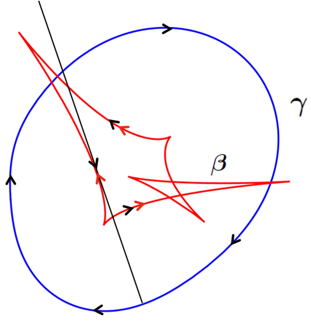
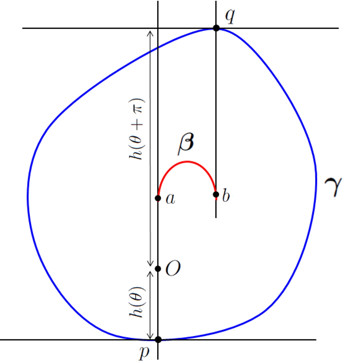
Figure 1: On the left the orientations of $\gamma$ (blue) and $\beta$ (red) as defined in the text, and on the right the figure for Proposition 3.

Lemma 1.

A segment of $\gamma$ between two vertices and the corresponding arc of $\beta$ have total curvatures equal in magnitude but opposite in sign.

Proof.

By ‘total curvature’ we mean the arc-length integral of the signed curvature. Let $s$ and $\sigma$ be the arc-length parameters of $\gamma$ and $\beta$ respectively. It is well known [26] that if $R=R(s)$ is the radius of curvature of $\gamma$ then the curvature of $\beta$ is $k_{\beta}=-1/(RR^{\prime})$ and $d\mbox{\boldmath$\beta$}/ds=R^{\prime}\mbox{\boldmath$N$}$ where $N$ is the unit normal to $\gamma$. Therefore

$$\int_{\sigma_{1}}^{\sigma_{2}}k_{\beta}d\sigma=\int_{s_{1}}^{s_{2}}\left(\frac{-1}{RR^{\prime}}\right)R^{\prime}ds=-\int_{s_{1}}^{s_{2}}\frac{1}{R}ds=-\int_{s_{1}}^{s_{2}}k_{\gamma}ds.$$

∎

Theorem 1.

Let $\gamma$ be a plane oval and $\beta$ its evolute. The rotation index of $\beta$, denoted $i$, is given by

$$i=(n-2)/2$$

where $n$ if the number of cusps of $\beta$ (or vertices of $\gamma$).

Proof.

The rotation index of $\beta$ is defined by $2\pi i=\int d\phi$ where $\phi$ is the angle the unit tangent vector to $\beta$ makes w.r.t. some fixed direction, thus

$$2\pi i=\sum_{j=1}^{n}\int_{\sigma_{j}}^{\sigma_{j+1}}k_{\beta}d\sigma+n\pi$$

where $j$ sums over the $n$ smooth arcs of $\beta$ and the $n$ cusps of $\beta$ are at $\sigma_{j}$. From Lemma 1 the first term on the right is just the total curvature of $\gamma$ which is $-2\pi$ because $\gamma$ is simple, smooth and oriented oppositely to $\beta$. Therefore

$$2\pi i=-2\pi+n\pi\qquad\implies\qquad i=(n-2)/2.$$ (2)

∎

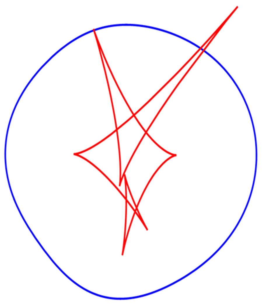
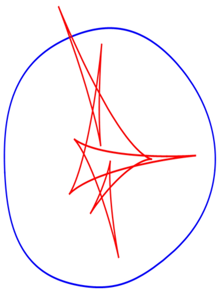
Figure 6: Examples of evolutes of plane curves. The left of Figure 1, together with the left and middle above, have $(i,n)=(2,6),(3,8),(4,10)$ in accordance with (2); the right is in accordance with (3).

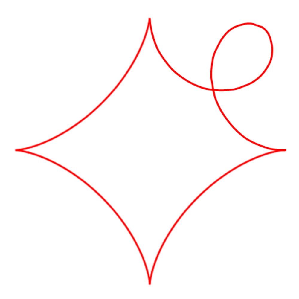
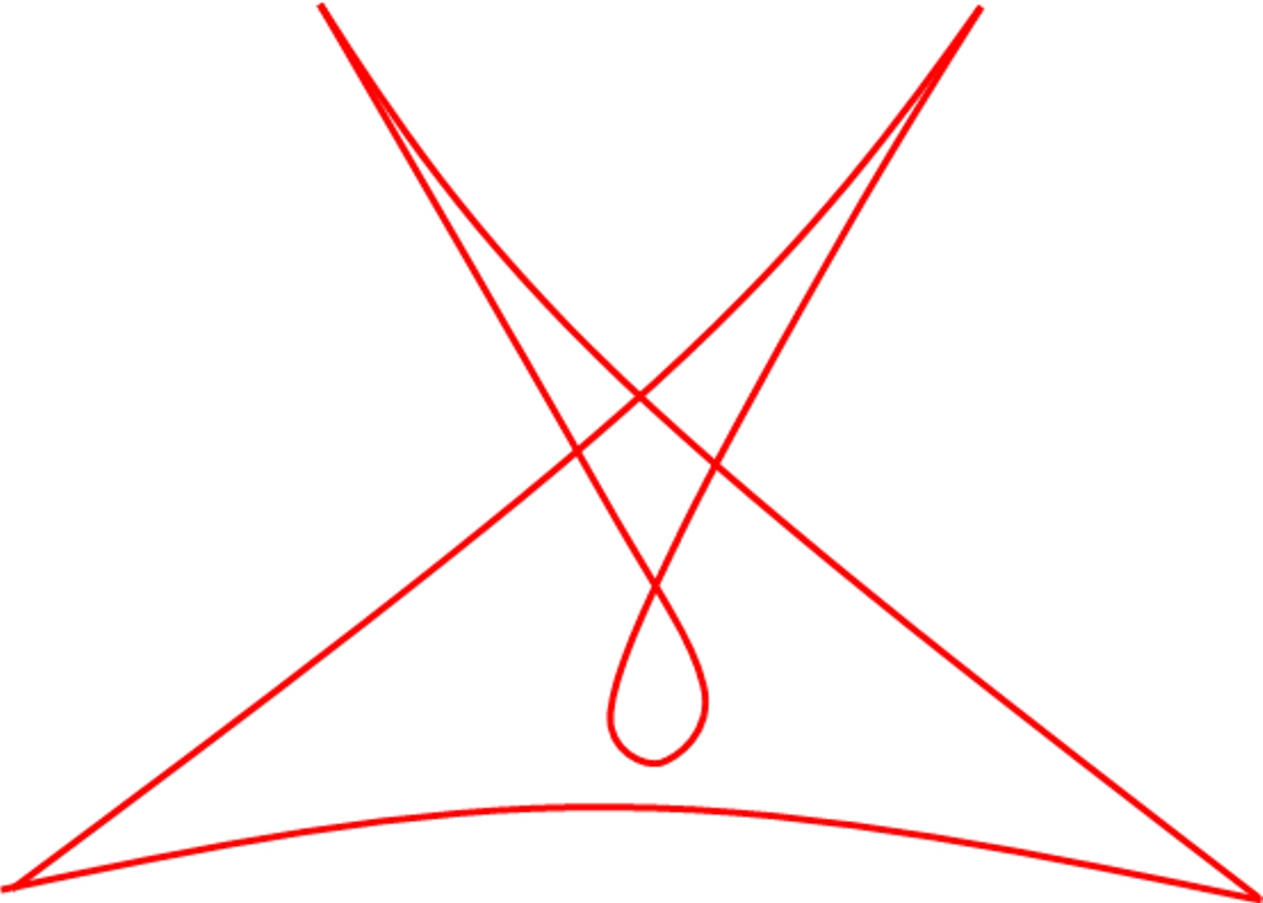
Figure 7: The left and middle cannot be the conjugate locus of a generic point on a convex surface; none can be the evolute of a plane oval.

This simple formula puts restrictions on the form the evolute of a plane oval can take, for example if the evolute is simple it can only have 4 cusps (see Figures 6 and 7 for examples). For the benefit of the next Section we will rephrase this result in more general terms:

It is useful to imagine the tangent line to $\beta$ rolling along the evolute in a smooth monotone way; this is due to the combination of local convexity of the smooth arcs and the ordinariness of the cusps. To make this more precise, let us define an ‘alternating’ orientation on $\beta$ by transporting the inward pointing normal to $\gamma$ along the normal line to where it is tangent to $\beta$ (red arrows in Figure 1), and let $t$ be the (unit) tangent vector to $\beta$ w.r.t. this orientation. The oriented tangent line defined by $t$ makes an angle $\Phi$ w.r.t. some fixed direction, but importantly this angle varies in a smooth and monotone way as we move along $\beta$ w.r.t. the standard orientation; in fact it changes by $-2\pi$ after one circuit of $\beta$ (this is because $\Phi$ is simply the angle made by the normal to $\gamma$, see Figure 1; this slightly overwrought description is necessary for later sections).

The rotation index of $\beta$ on the other hand is defined by the tangent vector w.r.t. the standard orientation. Let $T$ be this (unit) tangent vector and $\phi$ the angle it makes w.r.t. the same fixed direction. Since $\delta\phi=\pi$ at cusps then

$$2\pi i=\sum_{j=1}^{n}(\delta\phi)_{j}+n\pi$$

where $(\delta\phi)_{j}$ is the variation over the $j$th smooth arc. On the arcs where $\mbox{\boldmath$T$}=\mbox{\boldmath$t$}$ then $\delta\phi=\delta\Phi$, and on the arcs where $\mbox{\boldmath$T$}=-\mbox{\boldmath$t$}$ then $\phi=\Phi+\pi$ so again $\delta\phi=\delta\Phi$. Thus

$$2\pi i=\sum_{j=1}^{n}(\delta\Phi)_{j}+n\pi=-2\pi+n\pi\quad\implies\quad i=(n-2)/2.$$

In fact this is the case more generally, in the absence of any generating curve $\gamma$ or local convexity (without $\gamma$ some care is needed for point 2):

Theorem 2.

Let $\beta$ be a closed bounded piecewise-smooth planar curve with the following properties:

1. $\beta$ has an even number of smooth arcs separated by $n$ ordinary cusps,

2. the alternating oriented tangent line completes a single clockwise rotation in traversing $\beta$ w.r.t the standard orientation.

Then the rotation index of $\beta$ satisfies $i=(n-2)/2$.

It just happens that the evolute of a plane oval satisfies these conditions. Actually we can generalize to evolutes of plane curves with $k_{\gamma}\neq 0$ that are not simple: the term $\sum(\delta\phi)_{j}$ is just the rotation of the normal line to $\gamma$, so if $I$ is the rotation index of $\gamma$ then

$$i=(n+2I)/2.$$ (3)

As an example consider the well known evolute of a non-simple limaçon, where $i=-1,I=-2,n=2$ (see Figure 6 in the Appendix).

2.2 No smooth loops

While the evolute of a plane oval can have rotation index as high as we like and can be quite convoluted, we will show that any loops must have cusps on them; there can be no smooth loops. For this we use the support function [11], a useful notion surprisingly absent from many texts on Differential Geometry. Let $O$ be a point inside $\gamma$ and fix a direction. The line tangent to $\gamma$ at any point has an orthogonal segment to $O$ of length $h$ making an angle $\theta$ with the fixed direction. The $2\pi$-periodic function $h(\theta)$ is called the support function (well-defined since $\gamma$ is convex), and $\gamma$ is recovered from $h$ as follows: for each ray from $O$ making an angle $\theta$ w.r.t. some direction draw the line orthogonal to the ray a distance $h(\theta)$ from $O$; $\gamma$ is the envelope of these lines. The radius of curvature of $\gamma$ is simply $h^{\prime\prime}+h$, and hence a vertex of $\gamma$ occurs at a point $\theta$ where $h^{\prime\prime\prime}+h^{\prime}=0$. Since $h$ is a $2\pi$-periodic function we can represent it by a Fourier series, and the function $h^{\prime\prime\prime}+h^{\prime}$ has a Fourier series beginning at the second harmonic. The following is sometimes used in the proof of the 4-vertex theorem [26], we adapt it slightly.

Lemma 2.

Suppose $g$ is a $2\pi$-periodic function whose Fourier series begins at the second harmonic. Then any interval of length $\pi$ must contain a zero of $g$.

Proof.

Consider the functions $f$ and $g$ defined by the following differential equations:

$$f^{\prime\prime}=-4f,\qquad g^{\prime\prime}=-n^{2}g\quad n\geq 2.$$

By the Sturm comparison theorem [7] any interval between successive zeroes of $f$ must contain a zero of $g$. As the zeroes of $f$ are a distance $\pi/2$ apart, the zeroes of $g$ are at most a distance $\pi$ apart. Requiring $g$ to be $2\pi$-periodic gives a Fourier series beginning at the second harmonic. ∎

Theorem 3.

Let $\gamma$ be a plane oval, and $p$ a point on $\gamma$. There is a unique point $q$ on $\gamma$ such that the tangent lines at $p$ and $q$ are parallel. The points $p$ and $q$ divide $\gamma$ into two segments; there must be a vertex in each segment. In particular, if $\beta$ is the evolute of $\gamma$ then a smooth arc of $\beta$ cannot contain two parallel tangents.

Proof.

Let $O$ be on the normal to $\gamma$ at $p$ (see Figure 1). The angle made by the orthogonal ray from $O$ to the tangent lines at $p$ and $q$ differs by $\pi$. If there is no vertex between $p$ and $q$ then the derivative of the radius of curvature of $\gamma$ would have no zero in this interval, but since $h^{\prime\prime\prime}+h^{\prime}$ is a $2\pi$-periodic function whose Fourier series begins at the second harmonic then by Lemma 2 it must have a zero in any interval of length $\pi$, and the first statement follows. Now suppose $a$ and $b$ are two points on $\beta$ with parallel tangents (see Figure 1). If there are no cusps on the arc of $\beta$ between $a$ and $b$ then there is no vertex on the arc of $\gamma$ between $p$ and $q$, but since the tangents at $a$ and $b$ are parallel then the tangents at $p$ and $q$ are parallel and this contradicts the first statement. ∎

This ‘distribution’ of vertices/cusps can be formulated in a number of different ways:

Corollary 1.

Let $\gamma$ be a plane oval and $\beta$ its evolute.

1. If $a$ and $b$ are two points on a smooth arc of $\beta$ then $\int_{a}^{b}k_{\beta}d\sigma<\pi$.

2. Let $p$ be a point on $\gamma$ and $N$ the line normal to $\gamma$ at $p$. It is not possible for all the vertices of $\gamma$ to lie on one side of $N$.

3. It is not possible for $\beta$ to have a smooth loop, that is to say if $\mbox{\boldmath$\beta$}(\sigma_{1})=\mbox{\boldmath$\beta$}(\sigma_{2})$ and $\sigma_{1}\neq\sigma_{2}$, then $\beta$ has a cusp in $(\sigma_{1},\sigma_{2})$.

This is not to say we cannot construct a curve whose evolute has a smooth loop, or indeed a smooth ‘semicircle’ as point 1 above suggests, it is just that if we try to construct and close such a curve it will not be simple and convex (see Figure 6). In the next Section we will show how many, but not all, of these results carry over to the conjugate locus on convex surfaces.

3 Conjugate locus

Let $\mathcal{S}$ be a smooth strictly convex surface, and let $p$ be a point in $\mathcal{S}$. The conjugate locus of $p$ in $\mathcal{S}$, denoted $C_{p}$, is the envelope of geodesics emanating from $p$; put another way, $C_{p}$ is the set of all points conjugate to $p$ along geodesics emanating radially from $p$. We choose $\mathcal{S}$ to be strictly convex so every geodesic emanating from $p$ reaches a point conjugate to $p$ in finite distance; indeed if $K$ is the Gauss curvature of $\mathcal{S}$ then (again using Sturm’s comparison theorem, see [3],[17]) a conjugate point must be reached no sooner than $\pi/\sqrt{K_{max}}$ and no later than $\pi/\sqrt{K_{min}}$ (max/min w.r.t. $\mathcal{S}$ as a whole). Following Myers [21], we make the following definitions: fixing a direction in $T_{p}\mathcal{S}$, the (unit) tangent vector of a radial geodesic at $p$ makes an angle $\psi$ w.r.t. this direction and this radial geodesic reaches a conjugate point after a distance $R$. We call $R=R(\psi)$ the ‘distance function’ (another term being the ‘focal radius’, see [27]), and the polar curve it defines in $T_{p}\mathcal{S}$ the ‘distance curve’ (see Figure 2). The distance curve lies in the annulus of radii $(\pi/\sqrt{K_{max}},\pi/\sqrt{K_{min}})$ and is a smooth closed curve (star-shaped w.r.t. $p$); it is the exponential map of this curve (i.e. the conjugate locus) that is cusped (see Figure 2).

The following facts about the conjugate locus of a point $p$ are well known (see [10] or [30] for example): letting $\mbox{\boldmath$\Gamma$}_{\psi}(s)$ be the unit speed geodesic with $\mbox{\boldmath$\Gamma$}_{\psi}(0)=p$ and $\mbox{\boldmath$\Gamma$}_{\psi}^{\prime}(0)$ making an angle $\psi$ w.r.t. some fixed direction in $T_{p}\mathcal{S}$, we define the exponential map as $X:T_{p}\mathcal{S}\to\mathcal{S}:X(s,\psi)=\mbox{\boldmath$\Gamma$}_{\psi}(s)$. The Jacobi field $\mbox{\boldmath$J$}=\partial X/\partial\psi$ satisfies the Jacobi equation, which we can write in scalar form as follows (in general everything depends on $s,\psi$ but for brevity we only denote the functional dependence where necessary): letting $(\mbox{\boldmath$T$},\mbox{\boldmath$N$})$ be the unit tangent and normal to $\mbox{\boldmath$\Gamma$}_{\psi}(s)$ we write $\mbox{\boldmath$J$}=\xi\mbox{\boldmath$N$}+\eta\mbox{\boldmath$T$}$ and we can take $\eta=0$ w.l.o.g. (see [30]); then $\xi$ satisfies the scalar Jacobi equation

$$\frac{\partial^{2}\xi}{\partial s^{2}}+K\xi=0$$ (4)

where $K$ is evaluated along the radial geodesic and the partial derivatives are to emphasise that Jacobi fields vary along radial geodesics but also from one radial geodesic to another. With initial conditions $\xi(0,\psi)=0,\xi_{,s}(0,\psi)=1$ the first non-trivial zero of $\xi$ is a point conjugate to $p$. The distance curve is therefore defined implicilty by $\xi(R(\psi),\psi)=0$, and the conjugate locus in $\mathcal{S}$ is $X(R(\psi),\psi)$. Letting $\mbox{\boldmath$\beta$}(\psi):\mathbb{S}^{1}\to\mathcal{S}$ denote this parameterisation of $C_{p}$, then

$$\mbox{\boldmath$\beta$}^{\prime}=R^{\prime}(\psi)\mbox{\boldmath$T$}(R(\psi),\psi).$$ (5)

When $R$ is stationary then $\beta$ is not regular, it has a cusp (see Figure 2).

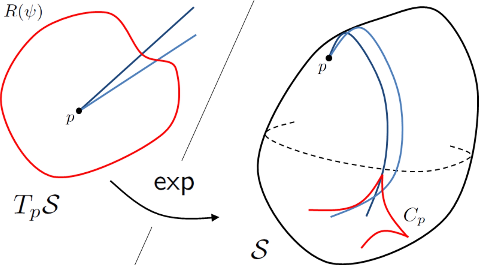
Figure 2: The distance curve in $T_{p}\mathcal{S}$ and its image in $\mathcal{S}$ under the exponential map: the conjugate locus of $p$, $C_{p}$.

It is worth noting that the last expression tells us the following: $R$ is the arc-length parameter of $C_{p}$; the length of an arc of $C_{p}$ is simply the difference between consecutive stationary values of $R$ and since $R$ lives in an annulus this can bound the total length of $C_{p}$; if we give an alternating signed length to $C_{p}$ then its total length is zero; and finally the ‘string’ construction of involutes carries over to conjugate loci (at $\psi_{1}$ move along a tangential geodesic a certain distance $\rho$, at $\psi_{2}$ move along a tangential geodesic a distance $\rho+R(\psi_{2})-R(\psi_{1})$; for some $\rho$ the involute will be a point, $p$).

3.1 Rotation index

In [30], the author derived an expression for the local structure of the conjugate locus by considering the higher derivatives of the exponential map, and we reproduce the formula here: let $q$ be a point on the conjugate locus corresponding to $\psi=\psi_{0}$ and suppose $R$ has an $A_{l}$ singularity at $\psi_{0}$, by which we mean the first $l$ derivatives of $R$ vanish but not the $(l+1)$th. Then the leading behaviour in the parameterization of the conjugate locus at $\psi=\psi_{0}+\delta\psi$ is

$$\mbox{\boldmath$T$}\left[R^{(l+1)}\frac{\delta\psi^{l+1}}{(l+1)!}+\ldots\right]+\mbox{\boldmath$N$}\left[(l+1)R^{(l+1)}\xi_{,s}\frac{\delta\psi^{l+2}}{(l+2)!}+\ldots\right].$$ (6)

We will return to the $\xi_{,s}$ term when we look at the geodesic curvature of $C_{p}$ (see (7)), for now we just need that $\xi_{,s}<0$. From this expression we see that if $R^{\prime}\neq 0$ (i.e. an $A_{0}$ singularity of $R$) then locally $C_{p}$ is a parabola opening in the direction of $N$ if $R^{\prime}<0$ and $-\mbox{\boldmath$N$}$ if $R^{\prime}>0$ (i.e. at regular points $C_{p}$ is locally convex), and if $R^{\prime}=0$ (but $R^{\prime\prime}\neq 0$, an $A_{1}$ singularity) then $C_{p}$ has an ordinary (semicubical parabola) cusp. We will describe a point $p$ in $\mathcal{S}$ as ‘generic’ if the distance function $R$ has at most $A_{1}$ singularities.

It is well known that the rotation index of a curve on a surface can be defined by that of its preimage w.r.t. the coordinate patch of the surface which contains the curve, indeed Hopf’s umlaufsatz does precisely that (see [9] or [19]). It is also well known that, with regards regular homotopy, every closed curve on a sphere has rotation index 0 or 1 [20]. For our purposes this is losing too much information about the curve, so (following Arnol’d [1]) we define the rotation index of the conjugate locus $C_{p}$ as that on the surface $\mathcal{S}$ with the point $p$ removed, which is equivalent to projecting the curve into a plane and finding the rotation index of that curve; we will essentially show this projected curve satisfies Theorem 2.

At the risk of confusing the reader we orient $\beta$ in the following way: at $q\in\mbox{\boldmath$\beta$}$ we move in such a way that the radial geodesic from $p$ which has conjugate point at $q$ lies to the right of $\beta$ w.r.t. the outward pointing normal of $\mathcal{S}$ (this uses the local convexity of $\beta$; alternatively $\psi$ increases in a clockwise sense when looking down on $p$, see Figure 5); this is so the orientation of the projected curve agrees with the previous Section, and so $C_{p}$ on the ellipsoid has $i=1$. Also, if a radial geodesic from $p$ has conjugate point at $q$, we will refer to the portion $[p,q]$ as a ‘geodesic segment’.

Theorem 4.

Let $\mathcal{S}$ be a smooth strictly convex surface and let $p$ be a generic point in $\mathcal{S}$. Then the conjugate locus of $p$ satisfies $i=(n-2)/2$, where $i$ is the rotation index of the conjugate locus in $\mathcal{S}/p$ and $n$ is the number of cusps.

Proof.

We already know the local structure of the conjugate locus of a generic point $p$ in $\mathcal{S}$: smooth arcs separated by ordinary cusps. Let $\Pi$ be the projection defined as follows: radially project from $p$ to the unique supporting plane of $\mathcal{S}$ parallel to the one at $p$. Since $\mathcal{S}$ is smooth and convex this projection $\Pi:\mathcal{S}/p\to\mathbb{R}^{2}$ is a homeomorphism. Letting $\mbox{\boldmath$\alpha$}=\Pi(\mbox{\boldmath$\beta$})$, then $\alpha$ is a piecewise-smooth curve with an even number of smooth arcs separated by ordinary cusps. If, on completing one circuit of $\alpha$, the tangent line turns through $2\pi I$, then from Section 2 we have $i=(n+2I)/2$ where $i$ is the rotation index of $\alpha$ in $\mathbb{R}^{2}$ (and hence the rotation index of $\beta$ in $\mathcal{S}/p$) and $n$ is the number of cusps to $\alpha$ (and also $\beta$). The only thing left to show is that $I=-1$.

Let $C_{\epsilon}$ be a small geodesic circle in $\mathcal{S}$ centred on $p$ with radius $\epsilon$. $\Pi(C_{\epsilon})$ will be a simple curve in $\mathbb{R}^{2}$ which approaches a (large) circle as $\epsilon\to 0$. The projection under $\Pi$ of a geodesic segment gives a semi-infinite curve in $\mathbb{R}^{2}$ which meets $\Pi(C_{\epsilon})$ at a unique point. For each $q\in\mbox{\boldmath$\beta$}$, we identify the tangent line to $\mbox{\boldmath$\alpha$}\in\mathbb{R}^{2}$ at $q^{\prime}=\Pi(q)$ with this point of intersection of $\Pi(C_{\epsilon})$ and the projected geodesic segment $[p,q]$. This identification is one-to-one and continuous, and since we traverse $\Pi(C_{\epsilon})$ once in rotating about $p$ then the tangent line to $\alpha$ makes one rotation and hence $I=\pm 1$. A simple diagram will show $I=-1$ with the orientations defined previously.

∎

An immediate corollary to this theorem would be an alternative route to proving the Last Geometric Statement of Jacobi: if we could show the conjugate locus of a generic point on the ellipsoid has rotation index 1 then there must be precisely 4 cusps.

3.2 Counting segments

In this section we will describe a way of assigning a positive intger to the regions of $\mathcal{S}$ (developing ideas in [26]) in order to give a convenient method of calculating the rotation index of $C_{p}$. We will use this, and the results of the previous section, to prove the ‘vierspitzensatz’: that the conjugate locus of a point on a convex surface must have at least 4 cusps. In a footnote, Myers [21] refers to Blaschke [3] (in German) who in turn credits Carathéodory with a proof of this statement (see also p.206 of [12]).

We define on the complement of $\beta$ in $\mathcal{S}$ the following (which we shall refer to as the ‘count’):

$$m(o):\mathcal{S}/\{\mbox{\boldmath$\beta$}\cup p\}\to\mathbb{N}/0$$

as the number of geodesic segments through the point $o\in\mathcal{S}/\mbox{\boldmath$\beta$}$ (we also exclude $p$ as the count is infinte there). The count is constant on each component of $\mathcal{S}/\mbox{\boldmath$\beta$}$, it is never equal to zero (see [21]), it is equal to 1 in the component of $\mathcal{S}/\mbox{\boldmath$\beta$}$ containing $p$ (see Figures 4 and 5 for examples) and it is preserved under the projection of the previous Subsection. As $o$ passes from one region of $\mathcal{S}/\mbox{\boldmath$\beta$}$ (or $\mathbb{R}^{2}/\mbox{\boldmath$\alpha$}$) to another the count changes according to the rules shown in Figure 3; we know this from the locally convex structure of $\beta$ described in (6).

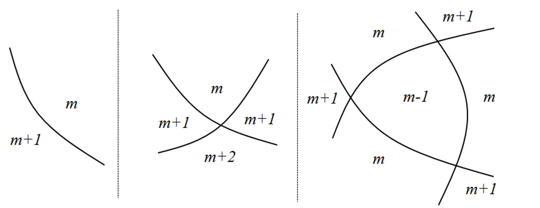
Figure 3: How the ‘count’ changes as we pass from one component of $\mathcal{S}/\mbox{\boldmath$\beta$}$ to another.

We note another way of defining the count: the exponential map of the interior of the distance curve will cover $\mathcal{S}$ and some points will be covered more than once; the number of times a point $o\in\mathcal{S}/\mbox{\boldmath$\beta$}$ is covered by this map is $m(o)$. This alternative formulation may be useful in Gauss-Bonnet type constructions [23].

We can use the count to describe a method of calculating the rotation index of $\beta$ due to McIntyre and Cairns [20]. In their paper they prove the following (we have adapted their statement to fit the current situation):

Theorem (McIntyre and Cairns).

Assigning a number to each region of $\mathcal{S}/\mbox{\boldmath$\beta$}$ according to the count, let $S_{m}$ be the union of the closure of the regions numbered $\geq m$, and $\chi_{m}$ the Euler characteristic of $S_{m}$. Then the rotation index of $\beta$ in $\mathcal{S}/p$ is

$$i=\sum_{m\geq 2}\chi_{m}.$$

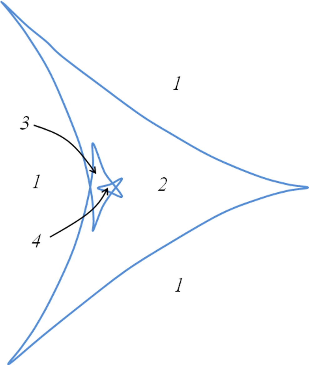
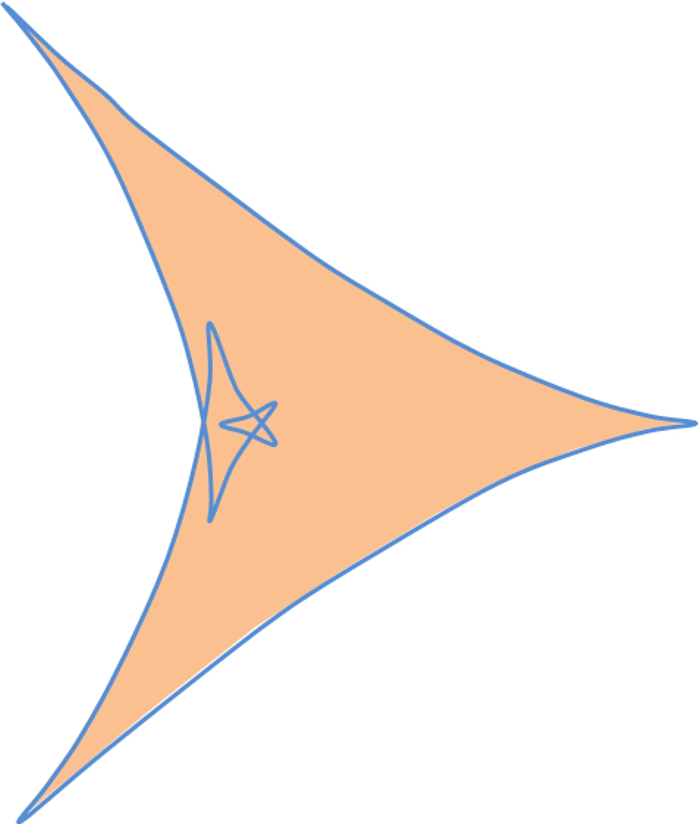
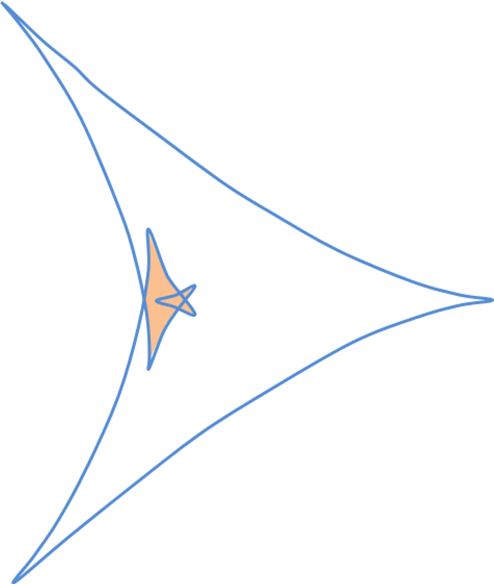
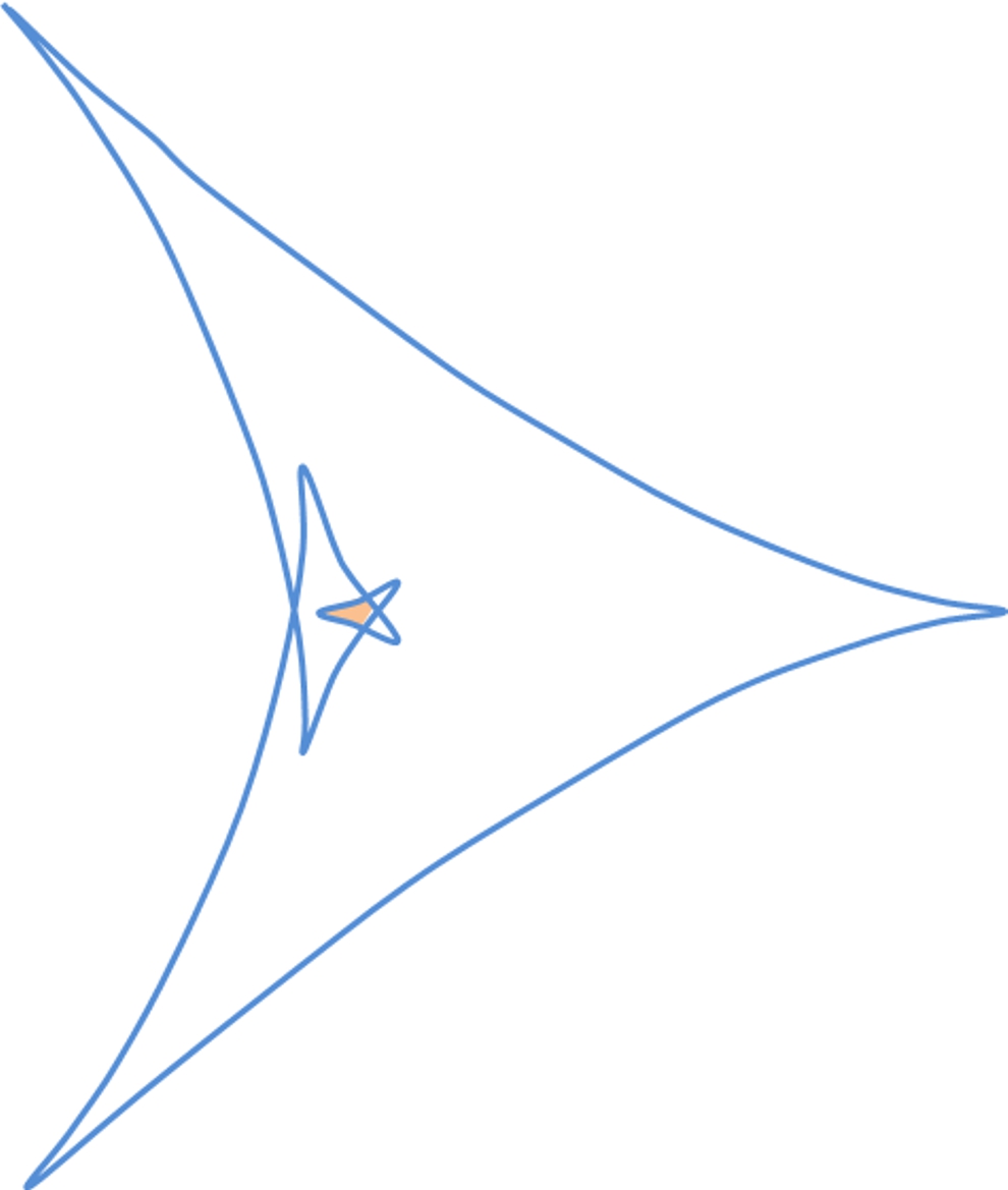
Figure 4: On the far left a typical conjugate locus (taken from [30]) with the count marked in some regions; then shaded are $S_{2},S_{3}$ and $S_{4}$, each of which are discs and have Euler charateristic 1. Thus the rotation index is 3, and the curve has 8 cusps as expected.

The example in Figure 4 is typical: the regions $S_{m}$ are usually discs or the disjoint union of discs, and hence have Euler characteristic $\geq 1$. If this were the case, the rotation index would be $\geq 1$ and hence $n$ could not be 2 via Theorem 4. Nonetheless, it is also possible that the $S_{m}$ are discs less discs, i.e. they could have ‘holes’:

Lemma 3.

For every hole in a region $S_{m}$, there is a disc.

Proof.

Suppose there is a region $S_{m}$ which has a hole; the count inside the hole must be $m-1$ (see the right of Figure 3 for an example). The boundary of the hole must contain points of self-intersection of $\beta$, as $\beta$ is connected, and the interior is star-shaped with repsect to any point in the interior, due to local convexity of $\beta$. If there is a point of self-intersection then there must be a sub-region of $S_{m}$ with count $m+1$. Either this region is a disc, in which case we are done, or it also has a hole. If it has a hole, then applying the same reasoning there must also be a region with count $m+2$, and so on. Eventually there must be a region without a hole, which is the disc we require. ∎

Theorem 5.

Let $\mathcal{S}$ be a smooth strictly convex surface and let $p$ be a generic point in $\mathcal{S}$. The conjugate locus of $p$ must have at least 4 cusps.

Proof.

According to Theorem 4, we must rule out the case of $\beta$ having rotation index 0 (if $p$ is generic then $R$ must have an even, and non-zero, number of stationary points which rules out $n=0,1,3$). But by Lemma 3 the sum of the Euler characteristics of the regions $S_{m}$ must be $\geq 1$, and hence the rotation index cannot be 0 and the number of cusps cannot be 2. ∎

3.3 No smooth loops

The rules of the count put other restrictions on $C_{p}$, for example: the conjugate locus cannot have any ‘necks’, by which we mean a point of intersection separating the conjugate locus into two non-overlapping components, and for any regular $q\in\mbox{\boldmath$\beta$}$ the locally convex side of $\beta$ (the side containing the geodesic segment $[p,q]$) cannot be the ‘outside’ (the component containing $p$). Continuing in this vein and in analogy with evolutes of plane ovals it might seem reasonable to expect a ‘no smooth loops’ statement to follow; however a counterexample would be the right of Figure 7 which satisfies all the requirements of the count and Theorem 4 and yet has a smooth loop.

Looking more deeply into the problem, suppose we view $R$, the distance curve in $T_{p}\mathcal{S}$, as the radius of curvature function of some plane curve $\tilde{\mbox{\boldmath$\gamma$}}$. From Theorem 5 $R$ has at least 4 stationary points and by the converse of the 4-vertex theorem [8] $\tilde{\mbox{\boldmath$\gamma$}}$ is therefore a simple closed curve; moreover it is strictly convex since $R>0$. The evolute of $\tilde{\mbox{\boldmath$\gamma$}}$, let’s call it $\tilde{\mbox{\boldmath$\beta$}}$, is a sort of dual to the conjugate locus, $\beta$. Both $\beta$ and $\tilde{\mbox{\boldmath$\beta$}}$ have the same number of cusps, and thus the same rotation index (in $\mathcal{S}/p$ and $\mathbb{R}^{2}$ respectively), and $\tilde{\mbox{\boldmath$\beta$}}$ has no smooth loops (by Corollary 1). This however is not enough to ensure $\beta$ cannot have any smooth loops, we give a counter example:

Up to now we have been studying the ‘first’ conjugate locus, where $R$ is the first non-trivial zero of $\xi$. We can extend this to consider the $j$th conjugate locus of a point $p$, denoted $C_{p}^{j}$, by simply letting $R$ be the $j$th non-trivial zero of $\xi$. Now each distance curve $R$ will have the same properties as described in the previous paragraph, however (as suggested in [24] and shown in Figure 5) the $j>1$ conjugate locus can have smooth loops. Indeed the annulus in $T_{p}\mathcal{S}$ that the distance curve lives in gets wider as $j$ increases and thus the lengths of the arcs of $C_{p}^{j}$ can be very long. Nonetheless, it seems likely to us that there can be no smooth loops in the first conjugate locus of a generic point on a smooth strictly convex surface, or to put it another way, an arc of $C_{p}$ cannot intersect itself.

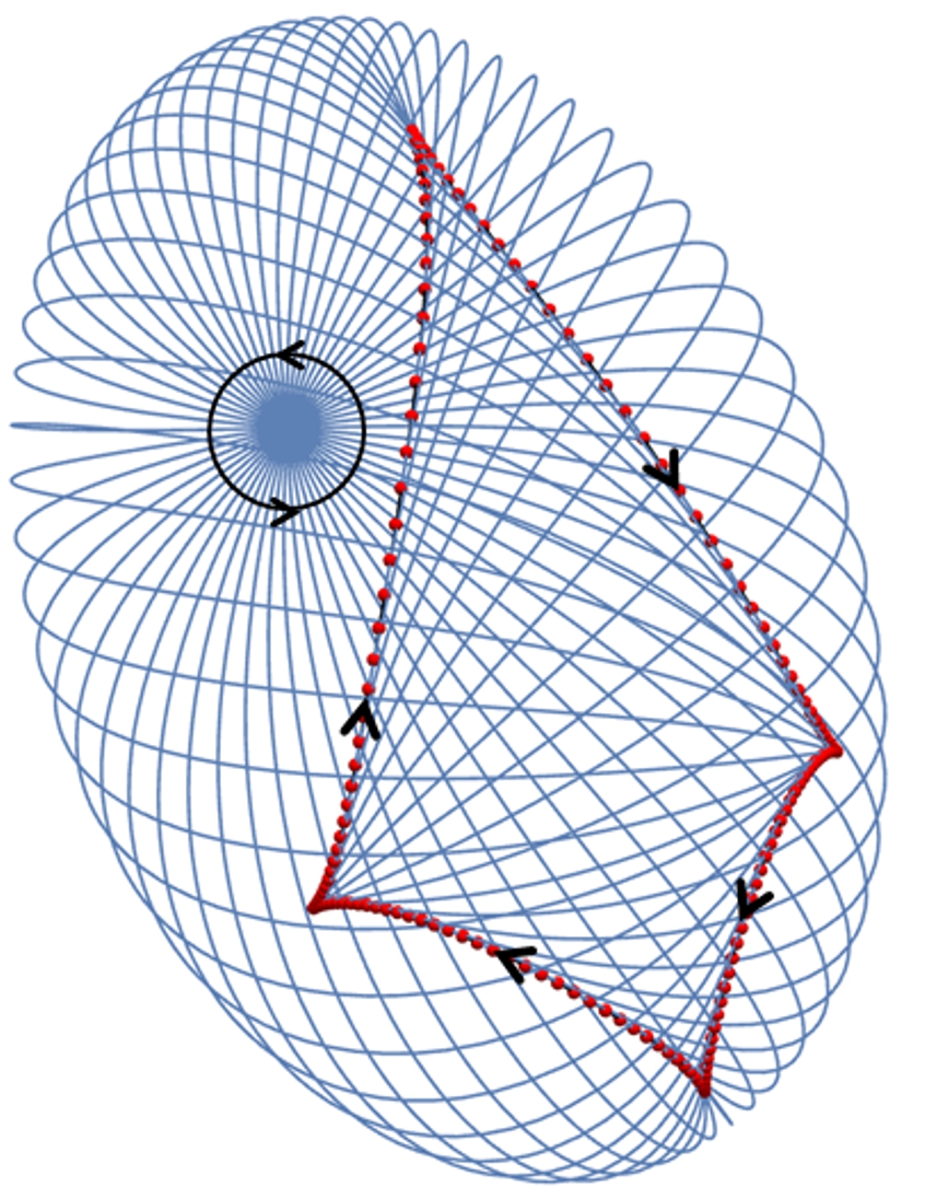
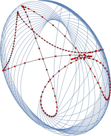
Figure 5: Examples of $C_{p}^{1}$ (left) and $C_{p}^{3}$ (right) on the triaxial ellipsoid. Note the four cusps on the left as predicted by the Itoh Kiyohara theorem, and the smooth loop on the right as described in the text. Blue lines are geodesics, black lines are the conjugate locus and the red dots are conjugate points.

3.4 Geodesic curvature

As it is relevant for this discussion, but seems to be missing from the literature, we derive an expression for the geodesic curvature of the conjugate locus. Recall from (5) that the unit tangent vector to $\mbox{\boldmath$\beta$}(\psi)$ is $\mbox{\boldmath$T$}(R(\psi),\psi)=\tfrac{\partial X}{\partial s}(R(\psi),\psi)$, so the $\psi$ derivative is

$$\frac{D}{d\psi}\mbox{\boldmath$T$}(R(\psi),\psi)=\frac{D\mbox{\boldmath$T$}}{\partial s}R^{\prime}+\frac{D}{\partial\psi}\frac{\partial X}{\partial s}=\frac{D}{\partial s}\frac{\partial X}{\partial\psi}=\frac{D}{\partial s}\mbox{\boldmath$J$}$$

since $D\mbox{\boldmath$T$}/\partial s=0$ by definiton of a geodesic. If $\mbox{\boldmath$J$}=\xi\mbox{\boldmath$N$}$ then $D\mbox{\boldmath$J$}/\partial s=\xi_{,s}\mbox{\boldmath$N$}$. Now letting $\sigma$ be the arc-length of $\beta$ the Frenet equation for geodesic curvature [18] gives

$$\frac{D}{d\sigma}\mbox{\boldmath$T$}=\frac{d\psi}{d\sigma}\frac{D}{d\psi}\mbox{\boldmath$T$}=\frac{1}{R^{\prime}}\xi_{,s}\mbox{\boldmath$N$}=k_{g}\mbox{\boldmath$N$}$$

and thus

$$k_{g}(\psi)=\frac{\xi_{,s}(R(\psi),\psi)}{R^{\prime}(\psi)}.$$ (7)

This explains the appearance of the $\xi_{,s}$ term in (6). We note that $\xi_{,s}(R(\psi),\psi)$ is never zero (and hence $k_{g}$ is never zero): since $R$ is defined by $\xi(R(\psi),\psi)=0$ then $\xi_{,s}(R(\psi),\psi)=0$ and the Jacobi equation (4) would imply $\xi\equiv 0$. Rather since $\xi_{,s}(0,\psi)=1$ and $s=R(\psi)$ is the first non-trivial zero of $\xi$ we have $\xi_{,s}(R(\psi),\psi)<0$. The formula applies equally well to $C_{p}^{j}$, if we simply adapt $R$ to be the $j$th non-trivial zero of $\xi$ (note the sign of $\xi_{,s}$ will alternate from $C_{p}^{j}$ to $C_{p}^{j+1}$). Another expression for the geodesic curvature is found by differentiating $\mbox{\boldmath$J$}(R(\psi),\psi)=0$ w.r.t. $\psi$ (see the ‘focal differential equation’ in [27]) to give $k_{g}=-\xi_{2}(R(\psi),\psi)/(R^{\prime})^{2}$ (see [30] for a definition of $\xi_{2}$).

Note the sign of $k_{g}$ in (7) alternates between positive and negative depending on whether $R$ is decreasing or increasing on an arc of $C_{p}$, whereas using the orientation defined before Theorem 4 in Section 3.1 $k_{g}$ is strictly positive; this is because (7) is derived w.r.t. the tangents to radial geodesics which define an alternating orientation on $C_{p}$, similar to that described in Section 2.1.

While the geodesic curvature in (7) diverges when $R$ is stationary (as we already knew), the total curvature

$$\int k_{g}d\sigma=\int\left(\frac{\xi_{,s}}{R^{\prime}}\right)R^{\prime}d\psi=\int\xi_{,s}(R(\psi),\psi)d\psi$$

does not depend explicitly on $R$. On the sphere $\xi_{,s}(R(\psi),\psi)=-1$, so on a perturbed sphere we might expect the total curvature of an arc of the conjugate locus to be close to the difference in the values of $\psi$ at which $R$ is stationary which suggests an upper bound on $\int k_{g}d\sigma$ (in line with Corrolary 1), however moving away from the sphere it seems the arcs of the conjugate locus can become very curved indeed.

4 Conclusions

We cannot simply draw a plane curve with an even number of arcs and cusps and claim it to be the evolute of a plane oval; there are restrictions both geometrical (local convexity, sum of the alternating lengths vanishing) and topological (rotation index, no smooth loops), as we have shown. In the same way we have shown that there are restrictions on the geometry and topology of the conjugate locus of a generic point on a smooth strictly convex surface, and these restrictions lead to structure which can be exploited.

There are a number of generalizations of the results in this paper which are worth considering. We have already alluded to the ‘higher’ conjugate locus $C_{p}^{j}$, and it is possible there is a formula generalizing (1). Also we remind the reader that the conjugate locus of $p$ is the envelope of geodesics normal to the geodesic circle centred on $p$ (in this context the term ‘caustic’ may be more appropriate). For small radius the geodesic circles are simple, and it is possible the caustics of simple curves on convex surfaces also satisfy (1) whereas nonsimple curves lead to (3) (possibly with the requirement the curves themselves have $k_{g}\neq 0$), however initial experiments suggest this context to be surprisingly complicated. Finally we have only considered convex surfaces however it is likely expressions such as (1) carry over to spheres with $K<0$ as long as the regions of negative Gauss curvature do not contain any closed geodesics (for example the spherical harmonic surfaces of [29], as opposed to the ‘dumbell’ of [25]).

Appendix A Additional diagrams

References

- [1] V. I. Arnol’d. The geometry of spherical curves and the algebra of quaternions. Russian Math. Surveys, 50(1):1–68, 1995.
- [2] M. Berger and B. Gostiaux. Differential Geometry: manifolds, curves, and surfaces. Springer-Verlag, 1988.
- [3] W. Blaschke. Vorlesungen über Differentialgeometrie, I: Elementare Differentialgeometrie. Springer, 1930.
- [4] B. Bonnard and J.-B. Caillau. Geodesic flow of the averaged controlled Kepler equation. Forum Mathematicum, 21(5):797–814, 2009.
- [5] B. Bonnard, J.-B. Caillau, R. Sinclair, and M. Tanaka. Conjugate and cut loci of a two-spere of revolution with application to optimal control. Ann. Inst. Henri Poincaré (C), 26(4):1081–1098, 2009.
- [6] J. W. Bruce and P. J. Giblin. Curves and singularities. Cambridge University Press, 1992.
- [7] E.A. Coddington and N. Levinson. Theory of Ordinary Differential Equations. Tata McGraw Hill, 1955.
- [8] D. DeTruck, H. Gluck, D. Pomerleano, and D. Shea Vick. The four vertex theorem and its converse. Notices of the AMS, 54(2):192–207, 2007.
- [9] M. P. DoCarmo. Differential Geometry of Curves and Surfaces. Prentice Hall, 1976.
- [10] M. P. DoCarmo. Riemannian Geometry. Birkhäuser, 1992.
- [11] D. Fuchs and S. Tabachnikov. Mathematical Omnibus: thirty lectures on classic Mathematics. American Mathematical Society, 2010.
- [12] M. Georgiadou. Constantin Carathéodory; mathematics and politics in turbulent times. Springer, 2004.
- [13] J.-I. Itoh and K. Kiyohara. The cut loci and the conjugate loci on ellipsoids. Manuscripta Mathematica, 114(2):247–264, 2004.
- [14] J.-I. Itoh and K. Kiyohara. The cut loci on ellipsoids and certain Liouville manifolds. Asian J. Math., 14(2):257–290, 2010.
- [15] J.-I. Itoh and K. Kiyohara. Cut loci and conjugate loci on Liouville surfaces. Manuscripta Mathematica, 136(1-2):115–141, 2011.
- [16] C. G. J. Jacobi. Vorlesungen über dynamik. Gehalten an der Universität zu Königsberg im Wintersemester 1842-1843 und nach einem von C. W. Borchart ausgearbeiteten hefte. hrsg. von A. Clebsch.
- [17] W. Klingenberg. Riemannian Geometry. De Gruyter, 1995.
- [18] W. Kühnel. Differential Geometry: curves - surfaces - manifolds. American Mathematical Society, 2006.
- [19] J. M. Lee. Riemannian Manifolds: an introduction to curvature. Springer-Verlag, 1997.
- [20] M. McIntyre and G. Cairns. A new formula for winding number. Geometriae Dedicata, 46:149–160, 1993.
- [21] S. B. Myers. Connections between differential geometry and topology, I: simply connected surfaces. Duke Math. J., 1(3):376–391, 1935.
- [22] H. Poincaré. Sur les lignes geodésiques des surfaces convexes. Trans. Am. Math. Soc., 17:237–274, 1905.
- [23] P. Røgen. Gauss-Bonnet’s theorem and closed Frenet frames. Geometriae Dedicata, 73:295–315, 1998.
- [24] R. Sinclair. On the last geometric statement of Jacobi. Experimental Mathematics, 12(4):477–485, 2003.
- [25] R. Sinclair and M. Tanaka. The cut locus of a two-sphere of revolution and Toponogov’s comparison theorem. Tohoku Math. J., 59:379–399, 2007.
- [26] S. Tabachnikov. Geometry and Billiards. American Mathematical Society, 2005.
- [27] H. Thielhelm, A. Vais, D. Brandes, and F-E. Wolter. Connecting geodesics on smooth surfaces. Vis. Comput., 28(6-8):529–539, 2012.
- [28] H. Thielhelm, A. Vais, and F-E. Wolter. Geodesic bifurcation on smooth surfaces. Vis. Comput., 31(2):187–204, 2015.
- [29] T. J. Waters. Regular and irregular geodesics on spherical harmonic surfaces. Physica D: Nonlinear Phenomena, 241(5):543–552, 2012.
- [30] T. J. Waters. Bifurcations of the conjugate locus. Journal of Geometry and Physics, 119:1–8, 2017.
- [31] H. Whitney. On regular closed curves in the plane. Compositio Mathematica, 4:276–284, 1937.