Accounting for model errors in iterative ensemble smoothers

Geir Evensen
Abstract

In the strong-constraint formulation of the history-matching problem, we assume that all the model errors relate to a selection of uncertain model input parameters. One does not account for additional model errors that could result from, e.g., excluded uncertain parameters, neglected physics in the model formulation, the use of an approximate model forcing, or discretization errors resulting from numerical approximations. If parameters with significant uncertainties are unaccounted for, there is a risk for an unphysical update, of some uncertain parameters, that compensates for errors in the omitted parameters. This paper gives the theoretical foundation for introducing model errors in ensemble methods for history matching. In particular, we explain procedures for practically including model errors in iterative ensemble smoothers like ESMDA and IES, and we demonstrate the impact of adding (or neglecting) model errors in the parameter-estimation problem. Also, we present a new result regarding the consistency of using the sample covariance of the predicted nonlinear measurements in the update schemes.

1 Introduction

It is standard to assume the model to be perfect when we use ensemble smoothers for solving inverse problems. This paper addresses the problem of consistently including the additional effect of stochastic model errors in different ensemble smoothers. In particular, we consider methods such as Ensemble Smoother (ES) (Evensen and van Leeuwen, 1996; Evensen, 2009b), Iterative ES (IES) (Chen and Oliver, 2012, 2013), and Ensemble Smoother with Multiple Data Assimilations (ESMDA) (Emerick and Reynolds, 2013).

There is a vast literature on solving the data-assimilation problem in the presence of model errors (see, e.g., the reviews by Carrassi and Vannitsem, 2016; Harlim, 2017). We traditionally characterize the data-assimilation problem as being either a weak-constraint or a strong-constraint problem, dependent on whether we include the dynamical model as a strong or a weak constraint in the cost function. The classical book by Bennett (1992) is entirely devoted to solving the weak-constraint inverse problem, and it illustrates that in the weak-constraint case we need to invert simultaneously for the state vector as a function of both space and time.

In Eknes and Evensen (1997) the variational formulation was solved for a weak-constraint parameter and state estimation problem using the representer method by Bennett (1992), and in Evensen (2003) different methods including ensemble methods were used to solve a weak-constraint state- and parameter-estimation problem. A conclusion from these works is that, if model errors are present, we need to increase the dimension of the problem by either updating the model solution as a function of space and time or by estimating the actual model errors and after that solve for the model solution. It is also interesting to realize that the simultaneous state-parameter estimation problem becomes nonlinear even if the model itself is linear (except for in a very trivial case), see for instance Evensen (2003). Also, when using Ensemble Kalman Filter (EnKF) by Evensen (1994) or ES, it is relatively easy to include stochastic model errors as long as we update both the parameters and the state variables simultaneously (Evensen, 2003, 2009a).

At this point, we should mention that we do not distinguish between model errors and model bias. In fact, with time-correlated stochastic model errors, and if the correlation becomes perfect (equal to one), then the model errors become equivalent to a constant bias. Fortunately, the procedure outlined in this paper can be used to estimate both model errors and model bias.

In a recent paper by Sakov etΒ al. (2018), the Iterative EnKF was reformulated to allow for additive model errors. However, for the history-matching problem, we need to account for more general representations of the error term since the solution of the reservoir simulator depends nonlinearly on the errors in the rate data used to force the model.

We will start by defining the standard strong-constraint history-matching problem, and after that, we move on to the general weak-constraint formulation. We then formally derive the ES, ESMDA, and IES, in the presence of model errors. The different smoother methods are used in a simple example to demonstrate the consistency of the formulation used and to illustrate the impact of model errors on the parameter-estimation problem.

2 Standard history-matching problem

The strong-constraint formulation given by Evensen (2018) is attractive because it simplifies the inverse problem and efficient ensemble smoothers can be defined. A first fundamental assumption is that we have a perfect deterministic forward model where the prediction 𝐲𝐲{\mathbf{y}} only depends on the input model parametrization 𝐱𝐱{\mathbf{x}},

𝐲=𝐠​(𝐱).𝐲𝐠𝐱{\mathbf{y}}={\mathbf{g}}({\mathbf{x}}). (1)

In a reservoir history-matching problem, the model operator is the reservoir simulation model, which predicts the observed production of oil, water, and gas, from the reservoir. Thus, given the true parametrization of 𝐱𝐱{\mathbf{x}}, the true prediction of 𝐲𝐲{\mathbf{y}} is precisely determined by the model in Eq. (1). Also, we have measurements 𝐝𝐝{\mathbf{d}} of the true 𝐲𝐲{\mathbf{y}} given as

𝐝=𝐲+𝐞.𝐝𝐲𝐞{\mathbf{d}}={\mathbf{y}}+{\mathbf{e}}. (2)

From evaluating the model operator 𝐠​(𝐱)𝐠𝐱{\mathbf{g}}({\mathbf{x}}), given a realization of the uncertain model parameters π±βˆˆβ„œn𝐱superscript𝑛{\mathbf{x}}\in\Re^{n}, we uniquely determine a realization of predicted measurements π²βˆˆβ„œm𝐲superscriptπ‘š{\mathbf{y}}\in\Re^{m} (corresponding to the real measurements πβˆˆβ„œm𝐝superscriptπ‘š{\mathbf{d}}\in\Re^{m}). Here n𝑛n is the number of parameters and mπ‘šm the number of measurements. We want to use the measurements to estimate the parameters 𝐱𝐱{\mathbf{x}}, and the measurements are assumed to contain random errors πžβˆˆβ„œm𝐞superscriptπ‘š{\mathbf{e}}\in\Re^{m}.

In history matching, it is common to define a prior distribution for the uncertain parameters since we usually will have more degrees of freedom in the parameters, than we have independent information in the measurements. Bayes’ theorem gives the joint posterior pdf for 𝐱𝐱{\mathbf{x}} and 𝐲𝐲{\mathbf{y}} as

f​(𝐱,𝐲|𝐝)∝f​(𝐱,𝐲)​f​(𝐝|𝐲)=f​(𝐱)​f​(𝐲|𝐱)​f​(𝐝|𝐲).proportional-to𝑓𝐱conditional𝐲𝐝𝑓𝐱𝐲𝑓conditional𝐝𝐲𝑓𝐱𝑓conditional𝐲𝐱𝑓conditional𝐝𝐲\begin{split}f({\mathbf{x}},{\mathbf{y}}\,|\,{\mathbf{d}})&\propto f({\mathbf{x}},{\mathbf{y}})f({\mathbf{d}}\,|\,{\mathbf{y}})\\ &=f({\mathbf{x}})f({\mathbf{y}}\,|\,{\mathbf{x}})f({\mathbf{d}}\,|\,{\mathbf{y}}).\end{split} (3)

In the case of no model errors, the transition density f​(𝐲|𝐱)𝑓conditional𝐲𝐱f({\mathbf{y}}\,|\,{\mathbf{x}}) becomes the Dirac delta function, and we can write

f​(𝐱,𝐲|𝐝)∝f​(𝐱)​δ​(π²βˆ’π β€‹(𝐱))​f​(𝐝|𝐲).proportional-to𝑓𝐱conditional𝐲𝐝𝑓𝐱𝛿𝐲𝐠𝐱𝑓conditional𝐝𝐲f({\mathbf{x}},{\mathbf{y}}\,|\,{\mathbf{d}})\propto f({\mathbf{x}})\delta({\mathbf{y}}-{\mathbf{g}}({\mathbf{x}}))f({\mathbf{d}}\,|\,{\mathbf{y}}). (4)

We are interested in the marginal pdf for 𝐱𝐱{\mathbf{x}}, which we obtain by integrating Eq. (4) over 𝐲𝐲{\mathbf{y}}, giving

f​(𝐱|𝐝)∝∫f​(𝐱)β€‹πœΉβ€‹(π²βˆ’π β€‹(𝐱))​f​(𝐝|𝐲)​d𝐲=f​(𝐱)​f​(𝐝|𝐠​(𝐱)).proportional-to𝑓conditionalπ±ππ‘“π±πœΉπ²π π±π‘“conditional𝐝𝐲differential-d𝐲𝑓𝐱𝑓conditional𝐝𝐠𝐱\begin{split}f({\mathbf{x}}\,|\,{\mathbf{d}})&\propto\int f({\mathbf{x}})\boldsymbol{\delta}({\mathbf{y}}-{\mathbf{g}}({\mathbf{x}}))f({\mathbf{d}}\,|\,{\mathbf{y}})\mathrm{d}{\mathbf{y}}\\ &=f({\mathbf{x}})f({\mathbf{d}}\,|\,{\mathbf{g}}({\mathbf{x}})).\end{split} (5)

When introducing the normal priors

f​(𝐱)𝑓𝐱\displaystyle f({\mathbf{x}}) =𝒩​(𝐱f,𝐂x​x),absent𝒩superscript𝐱fsubscript𝐂π‘₯π‘₯\displaystyle=\mathcal{N}({\mathbf{x}}^{\mathrm{f}},{\mathbf{C}}_{xx}), (6)
f​(𝐝|𝐠​(𝐱))=f​(𝐞)𝑓conditionalππ π±π‘“πž\displaystyle f({\mathbf{d}}\,|\,{\mathbf{g}}({\mathbf{x}}))=f({\mathbf{e}}) =𝒩​(𝟎,𝐂d​d),absent𝒩0subscript𝐂𝑑𝑑\displaystyle=\mathcal{N}({\mathbf{0}},{\mathbf{C}}_{dd}), (7)

we can write Eq.Β (5) as

f​(𝐱|𝐝)∝exp⁑{βˆ’12​(π±βˆ’π±f)T​𝐂x​xβˆ’1​(π±βˆ’π±f)}Γ—exp⁑{βˆ’12​(𝐠​(𝐱)βˆ’π)T​𝐂d​dβˆ’1​(𝐠​(𝐱)βˆ’π)}.proportional-to𝑓conditional𝐱𝐝12superscript𝐱superscript𝐱fTsubscriptsuperscript𝐂1π‘₯π‘₯𝐱superscript𝐱f12superscript𝐠𝐱𝐝Tsubscriptsuperscript𝐂1𝑑𝑑𝐠𝐱𝐝\begin{split}f({\mathbf{x}}\,|\,{\mathbf{d}})&\propto\exp\bigg{\{}-\frac{1}{2}\Big{(}{\mathbf{x}}-{\mathbf{x}}^{\mathrm{f}}\Big{)}^{\mathrm{T}}{\mathbf{C}}^{-1}_{xx}\Big{(}{\mathbf{x}}-{\mathbf{x}}^{\mathrm{f}}\Big{)}\bigg{\}}\\ &\times\exp\bigg{\{}-\frac{1}{2}\Big{(}{\mathbf{g}}({\mathbf{x}})-{\mathbf{d}}\Big{)}^{\mathrm{T}}{\mathbf{C}}^{-1}_{dd}\Big{(}{\mathbf{g}}({\mathbf{x}})-{\mathbf{d}}\Big{)}\bigg{\}}.\end{split} (8)

Note that the posterior pdf in Eq.Β (8) is non-Gaussian due to the nonlinear model 𝐠​(𝐱)𝐠𝐱{\mathbf{g}}({\mathbf{x}}). Maximizing f​(𝐱|𝐝)𝑓conditional𝐱𝐝f({\mathbf{x}}\,|\,{\mathbf{d}}) is equivalent to minimizing the cost function

π’₯​(𝐱)=(π±βˆ’π±f)T​𝐂x​xβˆ’1​(π±βˆ’π±f)+(𝐠​(𝐱)βˆ’π)T​𝐂d​dβˆ’1​(𝐠​(𝐱)βˆ’π).π’₯𝐱superscript𝐱superscript𝐱fTsuperscriptsubscript𝐂π‘₯π‘₯1𝐱superscript𝐱fsuperscript𝐠𝐱𝐝Tsuperscriptsubscript𝐂𝑑𝑑1𝐠𝐱𝐝\begin{split}\mathcal{J}({\mathbf{x}})&=\big{(}{\mathbf{x}}-{\mathbf{x}}^{\mathrm{f}}\big{)}^{\mathrm{T}}{\mathbf{C}}_{xx}^{-1}\big{(}{\mathbf{x}}-{\mathbf{x}}^{\mathrm{f}}\big{)}\\ &+\big{(}{\mathbf{g}}({\mathbf{x}})-{\mathbf{d}}\big{)}^{\mathrm{T}}{\mathbf{C}}_{dd}^{-1}\big{(}{\mathbf{g}}({\mathbf{x}})-{\mathbf{d}}\big{)}.\end{split} (9)

Most methods for history matching apply the assumptions of a perfect model and Gaussian priors, and they attempt to solve either one of Eqs.Β (8) or (9).

For this strong-constraint problem, Evensen (2018) explained how Eqs.Β (8) or (9) can be approximately solved using the ES, ESMDA, and IES. We can interpret these methods to approximately sample the posterior pdf in Eq.Β (8), and we can easily derive them as an ensemble of minimizing solutions of the cost function in Eq.Β (9) written for each realization as

π’₯​(𝐱j)=(𝐱jβˆ’π±jf)T​𝐂x​xβˆ’1​(𝐱jβˆ’π±jf)+(𝐠​(𝐱j)βˆ’πj)T​𝐂d​dβˆ’1​(𝐠​(𝐱j)βˆ’πj).π’₯subscript𝐱𝑗superscriptsubscript𝐱𝑗superscriptsubscript𝐱𝑗fTsuperscriptsubscript𝐂π‘₯π‘₯1subscript𝐱𝑗superscriptsubscript𝐱𝑗fsuperscript𝐠subscript𝐱𝑗subscript𝐝𝑗Tsuperscriptsubscript𝐂𝑑𝑑1𝐠subscript𝐱𝑗subscript𝐝𝑗\begin{split}\mathcal{J}({\mathbf{x}}_{j})&=\big{(}{\mathbf{x}}_{j}-{\mathbf{x}}_{j}^{\mathrm{f}}\big{)}^{\mathrm{T}}{\mathbf{C}}_{xx}^{-1}\big{(}{\mathbf{x}}_{j}-{\mathbf{x}}_{j}^{\mathrm{f}}\big{)}\\ &+\big{(}{\mathbf{g}}({\mathbf{x}}_{j})-{\mathbf{d}}_{j}\big{)}^{\mathrm{T}}{\mathbf{C}}_{dd}^{-1}\big{(}{\mathbf{g}}({\mathbf{x}}_{j})-{\mathbf{d}}_{j}\big{)}.\end{split} (10)

This approach relates to the papers on Ensemble Randomized Likelihood (EnRML) (Kitanidis, 1995; Oliver etΒ al., 1996). Note that the minimizing solutions will not precisely sample the posterior non-Gaussian distribution.

3 ES solution

We obtain the ES solution by first sampling the prior parameters 𝐱jfsuperscriptsubscript𝐱𝑗f{\mathbf{x}}_{j}^{\mathrm{f}} and the perturbed measurements 𝐝jsubscript𝐝𝑗{\mathbf{d}}_{j} from

𝐱jfsuperscriptsubscript𝐱𝑗f\displaystyle{\mathbf{x}}_{j}^{\mathrm{f}} βˆΌπ’©β€‹(𝐱f,𝐂x​x),similar-toabsent𝒩superscript𝐱fsubscript𝐂π‘₯π‘₯\displaystyle\sim\mathcal{N}({\mathbf{x}}^{\mathrm{f}},{\mathbf{C}}_{xx}), (11)
𝐝jsubscript𝐝𝑗\displaystyle{\mathbf{d}}_{j} βˆΌπ’©β€‹(𝐝,𝐂d​d).similar-toabsent𝒩𝐝subscript𝐂𝑑𝑑\displaystyle\sim\mathcal{N}({\mathbf{d}},{\mathbf{C}}_{dd}). (12)

We then compute the model predictions 𝐲jfsuperscriptsubscript𝐲𝑗f{\mathbf{y}}_{j}^{\mathrm{f}} from

𝐲jf=𝐠​(𝐱jf).superscriptsubscript𝐲𝑗f𝐠superscriptsubscript𝐱𝑗f{\mathbf{y}}_{j}^{\mathrm{f}}={\mathbf{g}}({\mathbf{x}}_{j}^{\mathrm{f}}). (13)

We define the covariance matrix between two vectors 𝐱𝐱{\mathbf{x}} and 𝐲𝐲{\mathbf{y}} as the expectation

𝐂x​y=𝔼​[(π±βˆ’π”Όβ€‹[𝐱])​(π²βˆ’π”Όβ€‹[𝐲])T],subscript𝐂π‘₯𝑦𝔼delimited-[]𝐱𝔼delimited-[]𝐱superscript𝐲𝔼delimited-[]𝐲T{\mathbf{C}}_{xy}=\mathbb{E}\left[\,\big{(}{\mathbf{x}}-\mathbb{E}\left[\,{\mathbf{x}}\,\right]\big{)}\big{(}{\mathbf{y}}-\mathbb{E}\left[\,{\mathbf{y}}\,\right]\big{)}^{\mathrm{T}}\,\right], (14)

while in the ensemble methods we introduce the sample mean

𝐱¯=1Nβ€‹βˆ‘j=1N𝐱j,¯𝐱1𝑁superscriptsubscript𝑗1𝑁subscript𝐱𝑗\overline{{\mathbf{x}}}=\frac{1}{N}\sum_{j=1}^{N}{\mathbf{x}}_{j}, (15)

and the sample covariance between two arbitrary vectors 𝐱𝐱{\mathbf{x}} and 𝐲𝐲{\mathbf{y}} as

𝐂¯x​y=1Nβˆ’1β€‹βˆ‘j=1N(𝐱jβˆ’π±Β―)​(𝐲jβˆ’π²Β―)T.subscript¯𝐂π‘₯𝑦1𝑁1superscriptsubscript𝑗1𝑁subscript𝐱𝑗¯𝐱superscriptsubscript𝐲𝑗¯𝐲T\overline{{\mathbf{C}}}_{xy}=\frac{1}{N-1}\sum_{j=1}^{N}\big{(}{\mathbf{x}}_{j}-\overline{{\mathbf{x}}}\big{)}\big{(}{\mathbf{y}}_{j}-\overline{{\mathbf{y}}}\big{)}^{\mathrm{T}}. (16)

Evensen (2018) derived the ES update equations for the parameters 𝐱jasuperscriptsubscript𝐱𝑗a{\mathbf{x}}_{j}^{\mathrm{a}} and the predictions 𝐲jasuperscriptsubscript𝐲𝑗a{\mathbf{y}}_{j}^{\mathrm{a}} as

𝐱jasuperscriptsubscript𝐱𝑗a\displaystyle{\mathbf{x}}_{j}^{\mathrm{a}} =𝐱jf+𝐂¯x​y​(𝐂¯y​y+𝐂d​d)βˆ’1​(𝐝jβˆ’π²jf),absentsuperscriptsubscript𝐱𝑗fsubscript¯𝐂π‘₯𝑦superscriptsubscript¯𝐂𝑦𝑦subscript𝐂𝑑𝑑1subscript𝐝𝑗superscriptsubscript𝐲𝑗f\displaystyle={\mathbf{x}}_{j}^{\mathrm{f}}+\overline{{\mathbf{C}}}_{xy}\left(\overline{{\mathbf{C}}}_{yy}+{\mathbf{C}}_{dd}\right)^{-1}\Big{(}{\mathbf{d}}_{j}-{\mathbf{y}}_{j}^{\mathrm{f}}\Big{)}, (17)
𝐲jasuperscriptsubscript𝐲𝑗a\displaystyle{\mathbf{y}}_{j}^{\mathrm{a}} =𝐠​(𝐱ja),absent𝐠superscriptsubscript𝐱𝑗a\displaystyle={\mathbf{g}}({\mathbf{x}}_{j}^{\mathrm{a}}), (18)

but see also the alternative derivation in Secs.Β 4.3–4.5 below regarding the consistency of using the sample covariance 𝐂¯y​ysubscript¯𝐂𝑦𝑦\overline{{\mathbf{C}}}_{yy} in Eq.Β (17). To compute the ES solution, we start from an initial ensemble of parameters 𝐱jfsuperscriptsubscript𝐱𝑗f{\mathbf{x}}_{j}^{\mathrm{f}} and perturbed measurements 𝐝jsubscript𝐝𝑗{\mathbf{d}}_{j}. First, we generate a prior ensemble prediction 𝐲jfsuperscriptsubscript𝐲𝑗f{\mathbf{y}}_{j}^{\mathrm{f}} by evaluating the model in Eq.Β (13) for each realization 𝐱jfsuperscriptsubscript𝐱𝑗f{\mathbf{x}}_{j}^{\mathrm{f}}. Then we compute the prior ensemble covariance between the parameters and the predicted measurements 𝐂¯x​yβˆˆβ„œnΓ—msubscript¯𝐂π‘₯𝑦superscriptπ‘›π‘š\overline{{\mathbf{C}}}_{xy}\in\Re^{n\times m} and the ensemble covariance of the predicted measurements 𝐂¯y​yβˆˆβ„œmΓ—msubscript¯𝐂𝑦𝑦superscriptπ‘šπ‘š\overline{{\mathbf{C}}}_{yy}\in\Re^{m\times m} and use them in the ES update in Eq.Β (17). Finally, we can recompute the model prediction using the updated parameters 𝐱jasuperscriptsubscript𝐱𝑗a{\mathbf{x}}_{j}^{\mathrm{a}} in Eq.Β (18).

As an alternative to solving the model in Eq.Β (18) for 𝐲jasuperscriptsubscript𝐲𝑗a{\mathbf{y}}_{j}^{\mathrm{a}}, it is possible to compute the updated prediction directly from an update equation

𝐲ja=𝐲jf+𝐂¯y​y​(𝐂¯y​y+𝐂d​d)βˆ’1​(𝐝jβˆ’π²jf),superscriptsubscript𝐲𝑗asuperscriptsubscript𝐲𝑗fsubscript¯𝐂𝑦𝑦superscriptsubscript¯𝐂𝑦𝑦subscript𝐂𝑑𝑑1subscript𝐝𝑗superscriptsubscript𝐲𝑗f{\mathbf{y}}_{j}^{\mathrm{a}}={\mathbf{y}}_{j}^{\mathrm{f}}+\overline{{\mathbf{C}}}_{yy}\left(\overline{{\mathbf{C}}}_{yy}+{\mathbf{C}}_{dd}\right)^{-1}\Big{(}{\mathbf{d}}_{j}-{\mathbf{y}}_{j}^{\mathrm{f}}\Big{)}, (19)

and in the case with a linear model, the result would be identical to solving Eq.Β (18). However, due to the nonlinearity of the deterministic model, the Eqs.Β (18) and (19) will give different results for 𝐲jasuperscriptsubscript𝐲𝑗a{\mathbf{y}}_{j}^{\mathrm{a}}. The Eq.Β (19) is just the standard ES update 𝐲jasuperscriptsubscript𝐲𝑗a{\mathbf{y}}_{j}^{\mathrm{a}} given the prior forecast ensemble for 𝐲jfsubscriptsuperscript𝐲f𝑗{\mathbf{y}}^{\mathrm{f}}_{j} and the perturbed measurements 𝐝jsubscript𝐝𝑗{\mathbf{d}}_{j} of 𝐲𝐲{\mathbf{y}}. We will later show that, for nonlinear models, there may be a benefit of computing 𝐲jasuperscriptsubscript𝐲𝑗a{\mathbf{y}}_{j}^{\mathrm{a}} indirectly through integration of the model in Eq.Β (18), initialized with 𝐱jasuperscriptsubscript𝐱𝑗a{\mathbf{x}}_{j}^{\mathrm{a}}, rather than using the direct update in Eq.Β (19). Also, the indirect update in Eq.Β (18) allows for the use of iterations.

4 General weak constraint problem

Lets now look at a formulation where we assume that the model depends nonlinearly on the model errors πͺπͺ{\mathbf{q}} as well as the parameters 𝐱𝐱{\mathbf{x}}, i.e.,

𝐲=𝐠​(𝐱,πͺ).𝐲𝐠𝐱πͺ{\mathbf{y}}={\mathbf{g}}({\mathbf{x}},{\mathbf{q}}). (20)

The model operator can be somewhat general, including a recursion or time steps, and the model error is a vector of noise components that could represent, e.g., the time-correlated noise in rate data used to force a reservoir simulation model over a specific period. Thus, there is a significant difference between 𝐱𝐱{\mathbf{x}} and πͺπͺ{\mathbf{q}}. Firstly, 𝐱𝐱{\mathbf{x}} is a static parameter that does not change with time. Thus, once the parameters 𝐱𝐱{\mathbf{x}} are estimated, we can use them in a future prediction simulation. The model errors πͺπͺ{\mathbf{q}}, on the other hand, will vary in time and are only estimated for the period of the inverse calculation. Only in the case of time-correlated errors can the estimated πͺπͺ{\mathbf{q}} be used to some extent as a forcing in the future prediction.

We assume that we have prior pdfs for the model errors and the parameters f​(𝐱)𝑓𝐱f({\mathbf{x}}) and f​(πͺ)𝑓πͺf({\mathbf{q}}). It is common, but not necessary, to assume that the model errors and parameters are independent so we can write the joint prior pdf as f​(𝐱,πͺ)=f​(𝐱)​f​(πͺ)𝑓𝐱πͺ𝑓𝐱𝑓πͺf({\mathbf{x}},{\mathbf{q}})=f({\mathbf{x}})f({\mathbf{q}}). The transition density for the model evolution is

f​(𝐲|𝐱,πͺ)=δ​(π²βˆ’π β€‹(𝐱,πͺ)),𝑓conditional𝐲𝐱πͺ𝛿𝐲𝐠𝐱πͺf({\mathbf{y}}|{\mathbf{x}},{\mathbf{q}})=\delta\big{(}{\mathbf{y}}-{\mathbf{g}}({\mathbf{x}},{\mathbf{q}})\big{)}, (21)

and we obtain the joint pdf by multiplying the prior with the transition density,

f​(𝐲,𝐱,πͺ)=δ​(π²βˆ’π β€‹(𝐱,πͺ))​f​(𝐱)​f​(πͺ).𝑓𝐲𝐱πͺ𝛿𝐲𝐠𝐱πͺ𝑓𝐱𝑓πͺf({\mathbf{y}},{\mathbf{x}},{\mathbf{q}})=\delta\big{(}{\mathbf{y}}-{\mathbf{g}}({\mathbf{x}},{\mathbf{q}})\big{)}f({\mathbf{x}})f({\mathbf{q}}). (22)

The likelihood function for the measurements given the prediction 𝐲𝐲{\mathbf{y}} is f​(𝐝|𝐲)𝑓conditional𝐝𝐲f({\mathbf{d}}|{\mathbf{y}}), thus, the posterior conditional pdf becomes

f​(𝐲,𝐱,πͺ|𝐝)∝f​(𝐝|𝐲)​δ​(π²βˆ’π β€‹(𝐱,πͺ))​f​(𝐱)​f​(πͺ).proportional-to𝑓𝐲𝐱conditionalπͺ𝐝𝑓conditional𝐝𝐲𝛿𝐲𝐠𝐱πͺ𝑓𝐱𝑓πͺf({\mathbf{y}},{\mathbf{x}},{\mathbf{q}}|{\mathbf{d}})\propto f({\mathbf{d}}|{\mathbf{y}})\delta\big{(}{\mathbf{y}}-{\mathbf{g}}({\mathbf{x}},{\mathbf{q}})\big{)}f({\mathbf{x}})f({\mathbf{q}}). (23)

Since 𝐲𝐲{\mathbf{y}} is given by the model in Eq.Β (20) as soon as we know 𝐱𝐱{\mathbf{x}} and πͺπͺ{\mathbf{q}}, we can compute the marginal density

f​(𝐱,πͺ|𝐝)∝∫f​(𝐝|𝐲)​δ​(π²βˆ’π β€‹(𝐱,πͺ))​f​(𝐱)​f​(πͺ)​d𝐲=f​(𝐝|𝐠​(𝐱,πͺ))​f​(𝐱)​f​(πͺ).proportional-to𝑓𝐱conditionalπͺ𝐝𝑓conditional𝐝𝐲𝛿𝐲𝐠𝐱πͺ𝑓𝐱𝑓πͺdifferential-d𝐲𝑓conditional𝐝𝐠𝐱πͺ𝑓𝐱𝑓πͺ\begin{split}f({\mathbf{x}},{\mathbf{q}}|{\mathbf{d}})&\propto\int f({\mathbf{d}}|{\mathbf{y}})\delta\big{(}{\mathbf{y}}-{\mathbf{g}}({\mathbf{x}},{\mathbf{q}})\big{)}f({\mathbf{x}})f({\mathbf{q}})\mathrm{d}{\mathbf{y}}\\ &=f\big{(}{\mathbf{d}}|{\mathbf{g}}({\mathbf{x}},{\mathbf{q}})\big{)}f({\mathbf{x}})f({\mathbf{q}}).\end{split} (24)

4.1 Gaussian priors

We now assume Gaussian priors

f​(𝐱)∝exp⁑{βˆ’12​(π±βˆ’π±f)T​𝐂x​xβˆ’1​(π±βˆ’π±f)},proportional-to𝑓𝐱12superscript𝐱superscript𝐱fTsuperscriptsubscript𝐂π‘₯π‘₯1𝐱superscript𝐱ff({\mathbf{x}})\propto\exp\bigg{\{}-\frac{1}{2}\big{(}{\mathbf{x}}-{\mathbf{x}}^{\mathrm{f}}\big{)}^{\mathrm{T}}{\mathbf{C}}_{xx}^{-1}\big{(}{\mathbf{x}}-{\mathbf{x}}^{\mathrm{f}}\big{)}\bigg{\}}, (25)

and

f​(πͺ)∝exp⁑{βˆ’12​(πͺβˆ’πͺf)T​𝐂q​qβˆ’1​(πͺβˆ’πͺf)},proportional-to𝑓πͺ12superscriptπͺsuperscriptπͺfTsuperscriptsubscriptπ‚π‘žπ‘ž1πͺsuperscriptπͺff({\mathbf{q}})\propto\exp\bigg{\{}-\frac{1}{2}\big{(}{\mathbf{q}}-{\mathbf{q}}^{\mathrm{f}}\big{)}^{\mathrm{T}}{\mathbf{C}}_{qq}^{-1}\big{(}{\mathbf{q}}-{\mathbf{q}}^{\mathrm{f}}\big{)}\bigg{\}}, (26)

where πͺfsuperscriptπͺf{\mathbf{q}}^{\mathrm{f}} would normally be zero. The likelihood for the measurements becomes

f(𝐝|𝐠(𝐱,πͺ))=exp⁑{βˆ’12​(𝐠​(𝐱,πͺ)βˆ’π)T​𝐂d​dβˆ’1​(𝐠​(𝐱,πͺ)βˆ’π)},𝑓|𝐝𝐠𝐱πͺ12superscript𝐠𝐱πͺ𝐝Tsuperscriptsubscript𝐂𝑑𝑑1𝐠𝐱πͺ𝐝\begin{split}f\big{(}{\mathbf{d}}&|{\mathbf{g}}({\mathbf{x}},{\mathbf{q}})\big{)}=\\ &\exp\bigg{\{}-\frac{1}{2}\big{(}{\mathbf{g}}({\mathbf{x}},{\mathbf{q}})-{\mathbf{d}}\big{)}^{\mathrm{T}}{\mathbf{C}}_{dd}^{-1}\big{(}{\mathbf{g}}({\mathbf{x}},{\mathbf{q}})-{\mathbf{d}}\big{)}\bigg{\}},\end{split} (27)

and we write the marginal posterior as

f​(𝐱,πͺ|𝐝)∝exp{βˆ’12​(π±βˆ’π±f)T​𝐂x​xβˆ’1​(π±βˆ’π±f)βˆ’12​(πͺβˆ’πͺf)T​𝐂q​qβˆ’1​(πͺβˆ’πͺf)βˆ’12(𝐠(𝐱,πͺ)βˆ’π)T𝐂d​dβˆ’1(𝐠(𝐱,πͺ)βˆ’π)}.proportional-to𝑓𝐱conditionalπͺ𝐝12superscript𝐱superscript𝐱fTsuperscriptsubscript𝐂π‘₯π‘₯1𝐱superscript𝐱f12superscriptπͺsuperscriptπͺfTsuperscriptsubscriptπ‚π‘žπ‘ž1πͺsuperscriptπͺf12superscript𝐠𝐱πͺ𝐝Tsuperscriptsubscript𝐂𝑑𝑑1𝐠𝐱πͺ𝐝\begin{split}f({\mathbf{x}},{\mathbf{q}}|{\mathbf{d}})\propto&\\ \exp\bigg{\{}&-\frac{1}{2}\big{(}{\mathbf{x}}-{\mathbf{x}}^{\mathrm{f}}\big{)}^{\mathrm{T}}{\mathbf{C}}_{xx}^{-1}\big{(}{\mathbf{x}}-{\mathbf{x}}^{\mathrm{f}}\big{)}\\ &-\frac{1}{2}\big{(}{\mathbf{q}}-{\mathbf{q}}^{\mathrm{f}}\big{)}^{\mathrm{T}}{\mathbf{C}}_{qq}^{-1}\big{(}{\mathbf{q}}-{\mathbf{q}}^{\mathrm{f}}\big{)}\\ &-\frac{1}{2}\big{(}{\mathbf{g}}({\mathbf{x}},{\mathbf{q}})-{\mathbf{d}}\big{)}^{\mathrm{T}}{\mathbf{C}}_{dd}^{-1}\big{(}{\mathbf{g}}({\mathbf{x}},{\mathbf{q}})-{\mathbf{d}}\big{)}\bigg{\}}.\end{split} (28)

Maximizing the posterior pdf in Eq.Β (28) is equivalent to minimizing the cost function

π’₯​(𝐱,πͺ)=(π±βˆ’π±f)T​𝐂x​xβˆ’1​(π±βˆ’π±f)+(πͺβˆ’πͺf)T​𝐂q​qβˆ’1​(πͺβˆ’πͺf)+(𝐠​(𝐱,πͺ)βˆ’π)T​𝐂d​dβˆ’1​(𝐠​(𝐱,πͺ)βˆ’π).π’₯𝐱πͺsuperscript𝐱superscript𝐱fTsuperscriptsubscript𝐂π‘₯π‘₯1𝐱superscript𝐱fsuperscriptπͺsuperscriptπͺfTsuperscriptsubscriptπ‚π‘žπ‘ž1πͺsuperscriptπͺfsuperscript𝐠𝐱πͺ𝐝Tsuperscriptsubscript𝐂𝑑𝑑1𝐠𝐱πͺ𝐝\begin{split}\mathcal{J}({\mathbf{x}},{\mathbf{q}})&=\big{(}{\mathbf{x}}-{\mathbf{x}}^{\mathrm{f}}\big{)}^{\mathrm{T}}{\mathbf{C}}_{xx}^{-1}\big{(}{\mathbf{x}}-{\mathbf{x}}^{\mathrm{f}}\big{)}\\ &+\big{(}{\mathbf{q}}-{\mathbf{q}}^{\mathrm{f}}\big{)}^{\mathrm{T}}{\mathbf{C}}_{qq}^{-1}\big{(}{\mathbf{q}}-{\mathbf{q}}^{\mathrm{f}}\big{)}\\ &+\big{(}{\mathbf{g}}({\mathbf{x}},{\mathbf{q}})-{\mathbf{d}}\big{)}^{\mathrm{T}}{\mathbf{C}}_{dd}^{-1}\big{(}{\mathbf{g}}({\mathbf{x}},{\mathbf{q}})-{\mathbf{d}}\big{)}.\end{split} (29)

As in the strong constraint case we sample the priors and define a cost function for each sample realization, and we obtain the weak constraint analog to the strong-constraint cost function in Eq.Β (10), i.e.,

π’₯​(𝐱j,πͺj)=(𝐱jβˆ’π±jf)T​𝐂x​xβˆ’1​(𝐱jβˆ’π±jf)+(πͺjβˆ’πͺjf)T​𝐂q​qβˆ’1​(πͺjβˆ’πͺjf)+(𝐠​(𝐱j,πͺj)βˆ’πj)T​𝐂d​dβˆ’1​(𝐠​(𝐱j,πͺj)βˆ’πj).π’₯subscript𝐱𝑗subscriptπͺ𝑗superscriptsubscript𝐱𝑗superscriptsubscript𝐱𝑗fTsuperscriptsubscript𝐂π‘₯π‘₯1subscript𝐱𝑗superscriptsubscript𝐱𝑗fsuperscriptsubscriptπͺ𝑗superscriptsubscriptπͺ𝑗fTsuperscriptsubscriptπ‚π‘žπ‘ž1subscriptπͺ𝑗superscriptsubscriptπͺ𝑗fsuperscript𝐠subscript𝐱𝑗subscriptπͺ𝑗subscript𝐝𝑗Tsuperscriptsubscript𝐂𝑑𝑑1𝐠subscript𝐱𝑗subscriptπͺ𝑗subscript𝐝𝑗\begin{split}\mathcal{J}({\mathbf{x}}_{j},{\mathbf{q}}_{j})&=\big{(}{\mathbf{x}}_{j}-{\mathbf{x}}_{j}^{\mathrm{f}}\big{)}^{\mathrm{T}}{\mathbf{C}}_{xx}^{-1}\big{(}{\mathbf{x}}_{j}-{\mathbf{x}}_{j}^{\mathrm{f}}\big{)}\\ &+\big{(}{\mathbf{q}}_{j}-{\mathbf{q}}_{j}^{\mathrm{f}}\big{)}^{\mathrm{T}}{\mathbf{C}}_{qq}^{-1}\big{(}{\mathbf{q}}_{j}-{\mathbf{q}}_{j}^{\mathrm{f}}\big{)}\\ &+\big{(}{\mathbf{g}}({\mathbf{x}}_{j},{\mathbf{q}}_{j})-{\mathbf{d}}_{j}\big{)}^{\mathrm{T}}{\mathbf{C}}_{dd}^{-1}\big{(}{\mathbf{g}}({\mathbf{x}}_{j},{\mathbf{q}}_{j})-{\mathbf{d}}_{j}\big{)}.\end{split} (30)

4.2 Stationarity condition

To develop a consistent set of equations for the different methods, it is simpler to rewrite the cost function for an augmented variable 𝐳T=(𝐱T,πͺT)superscript𝐳Tsuperscript𝐱TsuperscriptπͺT{\mathbf{z}}^{\mathrm{T}}=({\mathbf{x}}^{\mathrm{T}},{\mathbf{q}}^{\mathrm{T}}). We can then define the covariance

𝐂z​z=(𝐂x​x𝐂x​q𝐂q​x𝐂q​q),subscript𝐂𝑧𝑧matrixsubscript𝐂π‘₯π‘₯subscript𝐂π‘₯π‘žsubscriptπ‚π‘žπ‘₯subscriptπ‚π‘žπ‘ž{\mathbf{C}}_{zz}=\begin{pmatrix}{\mathbf{C}}_{xx}&{\mathbf{C}}_{xq}\\ {\mathbf{C}}_{qx}&{\mathbf{C}}_{qq}\end{pmatrix}, (31)

where we allow for correlations between 𝐱𝐱{\mathbf{x}} and πͺπͺ{\mathbf{q}} since this correlation becomes important in the iterative methods, and we can rewrite the cost function in Eq.Β (30) as

π’₯​(𝐳j)=(𝐳jβˆ’π³jf)T​𝐂z​zβˆ’1​(𝐳jβˆ’π³jf)+(𝐠​(𝐳j)βˆ’πj)T​𝐂d​dβˆ’1​(𝐠​(𝐳j)βˆ’πj).π’₯subscript𝐳𝑗superscriptsubscript𝐳𝑗superscriptsubscript𝐳𝑗fTsuperscriptsubscript𝐂𝑧𝑧1subscript𝐳𝑗superscriptsubscript𝐳𝑗fsuperscript𝐠subscript𝐳𝑗subscript𝐝𝑗Tsuperscriptsubscript𝐂𝑑𝑑1𝐠subscript𝐳𝑗subscript𝐝𝑗\begin{split}\mathcal{J}({\mathbf{z}}_{j})&=\big{(}{\mathbf{z}}_{j}-{\mathbf{z}}_{j}^{\mathrm{f}}\big{)}^{\mathrm{T}}{\mathbf{C}}_{zz}^{-1}\big{(}{\mathbf{z}}_{j}-{\mathbf{z}}_{j}^{\mathrm{f}}\big{)}\\ &+\big{(}{\mathbf{g}}({\mathbf{z}}_{j})-{\mathbf{d}}_{j}\big{)}^{\mathrm{T}}{\mathbf{C}}_{dd}^{-1}\big{(}{\mathbf{g}}({\mathbf{z}}_{j})-{\mathbf{d}}_{j}\big{)}.\end{split} (32)

This cost function is slightly more general than the one in Eq.Β (30) since we do not require independence betweeen πͺπͺ{\mathbf{q}} and 𝐱𝐱{\mathbf{x}}. By taking the gradient with respect to 𝐳jsubscript𝐳𝑗{\mathbf{z}}_{j} we obtain the following closed system of nonlinear equations for 𝐳jsubscript𝐳𝑗{\mathbf{z}}_{j}

𝐂z​zβˆ’1​(𝐳jβˆ’π³jf)superscriptsubscript𝐂𝑧𝑧1subscript𝐳𝑗superscriptsubscript𝐳𝑗f\displaystyle{\mathbf{C}}_{zz}^{-1}({\mathbf{z}}_{j}-{\mathbf{z}}_{j}^{\mathrm{f}}) +βˆ‡π³π β€‹(𝐳j)​𝐂d​dβˆ’1​(𝐠​(𝐳j)βˆ’πj)=0.subscriptβˆ‡π³π subscript𝐳𝑗superscriptsubscript𝐂𝑑𝑑1𝐠subscript𝐳𝑗subscript𝐝𝑗0\displaystyle+\nabla_{{\mathbf{z}}}{\mathbf{g}}({\mathbf{z}}_{j}){\mathbf{C}}_{dd}^{-1}\big{(}{\mathbf{g}}({\mathbf{z}}_{j})-{\mathbf{d}}_{j}\big{)}=0. (33)

In the case of a linear model, the solution is the standard Kalman filter update equation for the mean. However, the presence of the nonlinear function 𝐠​(𝐳j)𝐠subscript𝐳𝑗{\mathbf{g}}({\mathbf{z}}_{j}) makes the solution more elaborate. All of ES, ESMDA and IES are developed to solve this system of equations.

4.3 Derivation of ES update equations

To derive the ES solution, we will use a Taylor expansion and approximation that allows us to obtain a closed form solution for each realization of 𝐳jsubscript𝐳𝑗{\mathbf{z}}_{j}, i.e.,

𝐠​(𝐳j)𝐠subscript𝐳𝑗\displaystyle{\mathbf{g}}({\mathbf{z}}_{j}) =𝐠​(𝐳jf)+𝐆j​(𝐳jβˆ’π³jf),absent𝐠superscriptsubscript𝐳𝑗fsubscript𝐆𝑗subscript𝐳𝑗superscriptsubscript𝐳𝑗f\displaystyle={\mathbf{g}}({\mathbf{z}}_{j}^{\mathrm{f}})+{\mathbf{G}}_{j}({\mathbf{z}}_{j}-{\mathbf{z}}_{j}^{\mathrm{f}}), (34)

where we have defined

𝐆jTsuperscriptsubscript𝐆𝑗T\displaystyle{\mathbf{G}}_{j}^{\mathrm{T}} =βˆ‡π³π β€‹(𝐳)|𝐳=𝐳jf.absentevaluated-atsubscriptβˆ‡π³π π³π³superscriptsubscript𝐳𝑗f\displaystyle=\nabla_{\mathbf{z}}{\mathbf{g}}({\mathbf{z}})\big{|}_{{\mathbf{z}}={\mathbf{z}}_{j}^{\mathrm{f}}}. (35)

Thus, we approximate the nonlinear function 𝐠​(𝐳j)𝐠subscript𝐳𝑗{\mathbf{g}}({\mathbf{z}}_{j}) with its linearization in Eq.Β (34) around 𝐳=𝐳jf𝐳superscriptsubscript𝐳𝑗f{\mathbf{z}}={\mathbf{z}}_{j}^{\mathrm{f}} and in addition evaluate the gradient in Eq.Β (33) at 𝐳jfsuperscriptsubscript𝐳𝑗f{\mathbf{z}}_{j}^{\mathrm{f}}. We now have the gradient of the model, 𝐆jsubscript𝐆𝑗{\mathbf{G}}_{j} defined in Eq.Β (35), which differ for each realization. We wish to replace the individual model gradients with an β€œaveraged” gradient that is common for all realizations, and for now, we denote it 𝐆𝐆{\mathbf{G}}, which allows us to write Eq.Β (33) as

(𝐂z​zβˆ’1+𝐆T​𝐂d​dβˆ’1​𝐆)​(𝐳jβˆ’π³jf)superscriptsubscript𝐂𝑧𝑧1superscript𝐆Tsuperscriptsubscript𝐂𝑑𝑑1𝐆subscript𝐳𝑗superscriptsubscript𝐳𝑗f\displaystyle\big{(}{\mathbf{C}}_{zz}^{-1}+{\mathbf{G}}^{\mathrm{T}}{\mathbf{C}}_{dd}^{-1}{\mathbf{G}}\big{)}\big{(}{\mathbf{z}}_{j}-{\mathbf{z}}_{j}^{\mathrm{f}}\big{)} =𝐆T​𝐂d​dβˆ’1​(𝐝jβˆ’π β€‹(𝐳jf)).absentsuperscript𝐆Tsuperscriptsubscript𝐂𝑑𝑑1subscript𝐝𝑗𝐠superscriptsubscript𝐳𝑗f\displaystyle={\mathbf{G}}^{\mathrm{T}}{\mathbf{C}}_{dd}^{-1}\big{(}{\mathbf{d}}_{j}-{\mathbf{g}}({\mathbf{z}}_{j}^{\mathrm{f}})\big{)}. (36)

By solving for 𝐳jsubscript𝐳𝑗{\mathbf{z}}_{j} and using the matrix identity

(𝐆Tβ€‹πƒβˆ’1​𝐆+π‚βˆ’1)βˆ’1​𝐆Tβ€‹πƒβˆ’1=𝐂𝐆T​(𝐆𝐂𝐆T+𝐃)βˆ’1,superscriptsuperscript𝐆Tsuperscript𝐃1𝐆superscript𝐂11superscript𝐆Tsuperscript𝐃1superscript𝐂𝐆Tsuperscriptsuperscript𝐆𝐂𝐆T𝐃1\big{(}{\mathbf{G}}^{\mathrm{T}}{\mathbf{D}}^{-1}{\mathbf{G}}+{\mathbf{C}}^{-1}\big{)}^{-1}{\mathbf{G}}^{\mathrm{T}}{\mathbf{D}}^{-1}={\mathbf{C}}{\mathbf{G}}^{\mathrm{T}}\big{(}{\mathbf{G}}{\mathbf{C}}{\mathbf{G}}^{\mathrm{T}}+{\mathbf{D}}\big{)}^{-1}, (37)

(which can be derived from the Woodbury identity), where we substitute 𝐂z​zsubscript𝐂𝑧𝑧{\mathbf{C}}_{zz} for 𝐂𝐂{\mathbf{C}}, and 𝐂d​dsubscript𝐂𝑑𝑑{\mathbf{C}}_{dd} for 𝐃𝐃{\mathbf{D}}, we obtain the solution for 𝐳jsubscript𝐳𝑗{\mathbf{z}}_{j} as

𝐳jsubscript𝐳𝑗\displaystyle{\mathbf{z}}_{j} =𝐳jf+𝐂z​z​𝐆T​(𝐆𝐂z​z​𝐆T+𝐂d​d)βˆ’1​(𝐝jβˆ’π β€‹(𝐳jf)).absentsuperscriptsubscript𝐳𝑗fsubscript𝐂𝑧𝑧superscript𝐆Tsuperscriptsubscript𝐆𝐂𝑧𝑧superscript𝐆Tsubscript𝐂𝑑𝑑1subscript𝐝𝑗𝐠superscriptsubscript𝐳𝑗f\displaystyle={\mathbf{z}}_{j}^{\mathrm{f}}+{\mathbf{C}}_{zz}{\mathbf{G}}^{\mathrm{T}}\Big{(}{\mathbf{G}}{\mathbf{C}}_{zz}{\mathbf{G}}^{\mathrm{T}}+{\mathbf{C}}_{dd}\Big{)}^{-1}\Big{(}{\mathbf{d}}_{j}-{\mathbf{g}}({\mathbf{z}}_{j}^{\mathrm{f}})\Big{)}. (38)

4.4 Linear regression for 𝐆𝐆{\mathbf{G}}

Evensen (2018) used a Taylor expansion of 𝐠​(𝐳j)𝐠subscript𝐳𝑗{\mathbf{g}}({\mathbf{z}}_{j}) around the ensemble mean 𝐳¯=𝐳f¯𝐳superscript𝐳f\overline{{\mathbf{z}}}={\mathbf{z}}^{\mathrm{f}} and could then replace the individual gradients in Eq.Β (35) evaluated at 𝐳jsubscript𝐳𝑗{\mathbf{z}}_{j} with the gradient 𝐆𝐳¯subscript𝐆¯𝐳{\mathbf{G}}_{\overline{{\mathbf{z}}}} evaluated at the ensemble mean 𝐳¯¯𝐳\overline{{\mathbf{z}}}. He then showed that 𝐂¯z​yβ‰ˆπ†π³Β―β€‹π‚Β―z​zsubscript¯𝐂𝑧𝑦subscript𝐆¯𝐳subscript¯𝐂𝑧𝑧\overline{{\mathbf{C}}}_{zy}\approx{\mathbf{G}}_{\overline{{\mathbf{z}}}}\overline{{\mathbf{C}}}_{zz} and 𝐂¯y​yβ‰ˆπ†π³Β―β€‹π‚Β―z​z​𝐆𝐳¯Tsubscript¯𝐂𝑦𝑦subscript𝐆¯𝐳subscript¯𝐂𝑧𝑧superscriptsubscript𝐆¯𝐳T\overline{{\mathbf{C}}}_{yy}\approx{\mathbf{G}}_{\overline{{\mathbf{z}}}}\overline{{\mathbf{C}}}_{zz}{\mathbf{G}}_{\overline{{\mathbf{z}}}}^{\mathrm{T}} (Evensen, 2018, Eqs.Β 29 and Β 30), and he replaced the analytical gradients with ensemble covariances.

We will here use an interpretation based on linear regression (see also Reynolds etΒ al., 2006; Chen and Oliver, 2013) where we start by defining

π†β‰œπ‚y​z​𝐂z​zβˆ’1.β‰œπ†subscript𝐂𝑦𝑧superscriptsubscript𝐂𝑧𝑧1{\mathbf{G}}\triangleq{\mathbf{C}}_{yz}{\mathbf{C}}_{zz}^{-1}. (39)

Thus, we view 𝐆𝐆{\mathbf{G}} as the sensitivity matrix in a linear regression between 𝐲𝐲{\mathbf{y}} and 𝐳𝐳{\mathbf{z}} as

𝐂y​z=𝐆𝐂z​z.subscript𝐂𝑦𝑧subscript𝐆𝐂𝑧𝑧{\mathbf{C}}_{yz}={\mathbf{G}}{\mathbf{C}}_{zz}. (40)

When we introduce the ensemble-anomaly matrices

𝐘𝐘\displaystyle{\mathbf{Y}} =1Nβˆ’1​(𝐲1βˆ’π²Β―,…,𝐲Nβˆ’π²Β―)βˆˆβ„œmΓ—N,absent1𝑁1subscript𝐲1¯𝐲…subscript𝐲𝑁¯𝐲superscriptπ‘šπ‘\displaystyle=\frac{1}{\sqrt{N-1}}\big{(}{\mathbf{y}}_{1}-\overline{{\mathbf{y}}},\ldots,{\mathbf{y}}_{N}-\overline{{\mathbf{y}}}\big{)}\in\Re^{m\times N}, (41)
𝐙𝐙\displaystyle{\mathbf{Z}} =1Nβˆ’1​(𝐳1βˆ’π³Β―,…,𝐳Nβˆ’π³Β―)βˆˆβ„œnΓ—N,absent1𝑁1subscript𝐳1¯𝐳…subscript𝐳𝑁¯𝐳superscript𝑛𝑁\displaystyle=\frac{1}{\sqrt{N-1}}\big{(}{\mathbf{z}}_{1}-\overline{{\mathbf{z}}},\ldots,{\mathbf{z}}_{N}-\overline{{\mathbf{z}}}\big{)}\in\Re^{n\times N}, (42)

we can write Eq.Β (40) as

π˜π™Tβ‰ˆπ†π™π™T,superscriptπ˜π™Tsuperscript𝐆𝐙𝐙T{\mathbf{Y}}{\mathbf{Z}}^{\mathrm{T}}\approx{\mathbf{G}}{\mathbf{Z}}{\mathbf{Z}}^{\mathrm{T}}, (43)

or equivalently

π˜β‰ˆπ†π™,π˜π†π™{\mathbf{Y}}\approx{\mathbf{G}}{\mathbf{Z}}, (44)

where the approximation is the use of a finite ensemble size. From Eq.Β (39) we have

π†β‰ˆπ†Β―=𝐂¯y​z​(𝐂¯z​z)+=π˜π™T​(𝐙𝐙T)+=π˜π™+,𝐆¯𝐆subscript¯𝐂𝑦𝑧superscriptsubscript¯𝐂𝑧𝑧superscriptπ˜π™Tsuperscriptsuperscript𝐙𝐙Tsuperscriptπ˜π™\begin{split}{\mathbf{G}}&\approx\overline{{\mathbf{G}}}=\overline{{\mathbf{C}}}_{yz}(\overline{{\mathbf{C}}}_{zz})^{+}={\mathbf{Y}}{\mathbf{Z}}^{\mathrm{T}}\big{(}{\mathbf{Z}}{\mathbf{Z}}^{\mathrm{T}}\big{)}^{+}={\mathbf{Y}}{\mathbf{Z}}^{+},\end{split} (45)

where the superscript + denotes pseudo inverse. The unbiasedness of 𝐆¯¯𝐆\overline{{\mathbf{G}}} can be shown, i.e.,

𝔼​[𝐆¯]=𝐆.𝔼delimited-[]¯𝐆𝐆\mathbb{E}\left[\,\overline{{\mathbf{G}}}\,\right]={\mathbf{G}}. (46)

Also, using Eq.Β (39), we can write

𝐆𝐂z​z​𝐆T=𝐂y​z​𝐂z​zβˆ’1​𝐂z​y,subscript𝐆𝐂𝑧𝑧superscript𝐆Tsubscript𝐂𝑦𝑧superscriptsubscript𝐂𝑧𝑧1subscript𝐂𝑧𝑦{\mathbf{G}}{\mathbf{C}}_{zz}{\mathbf{G}}^{\mathrm{T}}={\mathbf{C}}_{yz}{\mathbf{C}}_{zz}^{-1}{\mathbf{C}}_{zy}, (47)

and when we introduce the ensemble representation from Eq.Β (45), we obtain

𝐆¯​𝐂¯z​z​𝐆¯T=π˜β€‹(𝐙+​𝐙)​(𝐙+​𝐙)β€‹π˜T.¯𝐆subscript¯𝐂𝑧𝑧superscript¯𝐆T𝐘superscript𝐙𝐙superscript𝐙𝐙superscript𝐘T\begin{split}\overline{{\mathbf{G}}}\;\overline{{\mathbf{C}}}_{zz}\overline{{\mathbf{G}}}^{\mathrm{T}}&={\mathbf{Y}}({\mathbf{Z}}^{+}{\mathbf{Z}})({\mathbf{Z}}^{+}{\mathbf{Z}}){\mathbf{Y}}^{\mathrm{T}}.\end{split} (48)

The projection 𝐙+​𝐙superscript𝐙𝐙{\mathbf{Z}}^{+}{\mathbf{Z}} is just the orthogonal projection onto the range of 𝐙Tsuperscript𝐙T{\mathbf{Z}}^{\mathrm{T}}. We will now consider three cases:

4.4.1 Linear model and measurement operator

For a linear model and measurement operator we can write, e.g., 𝐘=π‡π™π˜π‡π™{\mathbf{Y}}={\mathbf{H}}{\mathbf{Z}}, and Eq.Β (48) becomes

𝐆¯​𝐂¯z​z​𝐆¯T=𝐇𝐙​(𝐙+​𝐙)​(𝐙+​𝐙)​𝐙T​𝐇T=𝐇𝐙​(𝐇𝐙)T=𝐘𝐘T=𝐂¯y​y.¯𝐆subscript¯𝐂𝑧𝑧superscript¯𝐆T𝐇𝐙superscript𝐙𝐙superscript𝐙𝐙superscript𝐙Tsuperscript𝐇T𝐇𝐙superscript𝐇𝐙Tsuperscript𝐘𝐘Tsubscript¯𝐂𝑦𝑦\begin{split}\overline{{\mathbf{G}}}\;\overline{{\mathbf{C}}}_{zz}\overline{{\mathbf{G}}}^{\mathrm{T}}&={\mathbf{H}}{\mathbf{Z}}({\mathbf{Z}}^{+}{\mathbf{Z}})({\mathbf{Z}}^{+}{\mathbf{Z}}){\mathbf{Z}}^{\mathrm{T}}{\mathbf{H}}^{\mathrm{T}}\\ &={\mathbf{H}}{\mathbf{Z}}({\mathbf{H}}{\mathbf{Z}})^{\mathrm{T}}={\mathbf{Y}}{\mathbf{Y}}^{\mathrm{T}}=\overline{{\mathbf{C}}}_{yy}.\end{split} (49)

Hence, Eq.Β (49) is consistent with the definition of the covariance matrix 𝐂¯y​y=𝐘𝐘Tsubscript¯𝐂𝑦𝑦superscript𝐘𝐘T\overline{{\mathbf{C}}}_{yy}={\mathbf{Y}}{\mathbf{Y}}^{\mathrm{T}} for linear models and all combinations of n𝑛n and N𝑁N.

4.4.2 Nonlinear model and nβ‰₯Nβˆ’1𝑛𝑁1n\geq N-1

In the case with a nonlinear model and nβ‰₯Nβˆ’1𝑛𝑁1n\geq N-1 the rank of 𝐙𝐙{\mathbf{Z}} is Nβˆ’1𝑁1N-1, and the projection 𝐙+​𝐙=(πˆβˆ’1Nβ€‹πŸπŸT)superscriptπ™π™πˆ1𝑁superscript11T{\mathbf{Z}}^{+}{\mathbf{Z}}=\Big{(}{\mathbf{I}}-\frac{1}{N}\mathbf{1}\mathbf{1}^{\mathrm{T}}\Big{)} with πŸβˆˆβ„œN1superscript𝑁\mathbf{1}\in\Re^{N} being a vector with all elements equal to one (see the Appendix in Sakov etΒ al., 2012). This result is seen from the fact that 𝐙𝐙{\mathbf{Z}} has only one singular value equal to zero corresponding to the right singular vector 𝟏/N1𝑁\mathbf{1}/\sqrt{N}. The projection 𝐙+​𝐙superscript𝐙𝐙{\mathbf{Z}}^{+}{\mathbf{Z}} is then just the subtraction of the ensemble mean. Since we have already removed the ensemble mean from 𝐘𝐘{\mathbf{Y}}, we can write Eq.Β (48) as

𝐆¯​𝐂¯z​z​𝐆¯T=π˜β€‹(πˆβˆ’1Nβ€‹πŸπŸT)​(πˆβˆ’1Nβ€‹πŸπŸT)β€‹π˜T=𝐘𝐘T=𝐂¯y​y,¯𝐆subscript¯𝐂𝑧𝑧superscript¯𝐆T𝐘𝐈1𝑁superscript11T𝐈1𝑁superscript11Tsuperscript𝐘Tsuperscript𝐘𝐘Tsubscript¯𝐂𝑦𝑦\begin{split}\overline{{\mathbf{G}}}\;\overline{{\mathbf{C}}}_{zz}\overline{{\mathbf{G}}}^{\mathrm{T}}&={\mathbf{Y}}\Big{(}{\mathbf{I}}-\frac{1}{N}\mathbf{1}\mathbf{1}^{\mathrm{T}}\Big{)}\Big{(}{\mathbf{I}}-\frac{1}{N}\mathbf{1}\mathbf{1}^{\mathrm{T}}\Big{)}{\mathbf{Y}}^{\mathrm{T}}\\ &={\mathbf{Y}}{\mathbf{Y}}^{\mathrm{T}}=\overline{{\mathbf{C}}}_{yy},\end{split} (50)

and as in the linear case, Eq.Β (48) exactly corresponds to the definition of the ensemble covariance 𝐂¯y​ysubscript¯𝐂𝑦𝑦\overline{{\mathbf{C}}}_{yy}. This nonlinear case with nβ‰₯Nβˆ’1𝑛𝑁1n\geq N-1 is the most considered case for history matching, data assimilation with nonlinear measurement operators, and iterative smoothers used for sequential data assimilation in nonlinear models. Thus, for most applications of ensemble methods, we can replace the product 𝐆¯​𝐂¯z​z​𝐆¯T¯𝐆subscript¯𝐂𝑧𝑧superscript¯𝐆T\overline{{\mathbf{G}}}\;\overline{{\mathbf{C}}}_{zz}\overline{{\mathbf{G}}}^{\mathrm{T}} with the sample covariance 𝐂¯y​ysubscript¯𝐂𝑦𝑦\overline{{\mathbf{C}}}_{yy}.

4.4.3 Nonlinear model and n<Nβˆ’1𝑛𝑁1n<N-1

In the case of a nonlinear model and n<Nβˆ’1𝑛𝑁1n<N-1, which applies for the example considered in SectionΒ 6, the expression in Eq.Β (48) is not equal to 𝐘𝐘Tsuperscript𝐘𝐘T{\mathbf{Y}}{\mathbf{Y}}^{\mathrm{T}} and we must include the projection and redefine the sample covariance as

𝐂~y​yβ‰œπ˜β€‹(𝐙+​𝐙)​(π˜β€‹(𝐙+​𝐙))T,β‰œsubscript~π‚π‘¦π‘¦π˜superscript𝐙𝐙superscript𝐘superscript𝐙𝐙T\begin{split}\widetilde{{\mathbf{C}}}_{yy}&\triangleq{\mathbf{Y}}({\mathbf{Z}}^{+}{\mathbf{Z}})\big{(}{\mathbf{Y}}({\mathbf{Z}}^{+}{\mathbf{Z}})\big{)}^{\mathrm{T}},\end{split} (51)

i.e., we compute the covariance of the predicted measurement anomalies projected onto the range of 𝐙Tsuperscript𝐙T{\mathbf{Z}}^{\mathrm{T}}. This case also applies for nonlinear models in the limit of infinite ensemble size. Thus, we must use the definition Eq.Β (51) to evaluate 𝐂~y​ysubscript~𝐂𝑦𝑦\widetilde{{\mathbf{C}}}_{yy} to ensure consistency in the derivation of the update equation.

4.5 ES algorithm

We can replace the gradient 𝐆𝐆{\mathbf{G}} in the update Eq.Β (38), using Eqs.Β (40) and (47) to obtain

𝐳jasuperscriptsubscript𝐳𝑗a\displaystyle{\mathbf{z}}_{j}^{\mathrm{a}} =𝐳jf+𝐂z​y​(𝐂y​z​𝐂z​zβˆ’1​𝐂z​y+𝐂d​d)βˆ’1​(𝐝jβˆ’π β€‹(𝐳jf)).absentsuperscriptsubscript𝐳𝑗fsubscript𝐂𝑧𝑦superscriptsubscript𝐂𝑦𝑧superscriptsubscript𝐂𝑧𝑧1subscript𝐂𝑧𝑦subscript𝐂𝑑𝑑1subscript𝐝𝑗𝐠superscriptsubscript𝐳𝑗f\displaystyle={\mathbf{z}}_{j}^{\mathrm{f}}+{\mathbf{C}}_{zy}\Big{(}{\mathbf{C}}_{yz}{\mathbf{C}}_{zz}^{-1}{\mathbf{C}}_{zy}+{\mathbf{C}}_{dd}\Big{)}^{-1}\Big{(}{\mathbf{d}}_{j}-{\mathbf{g}}({\mathbf{z}}_{j}^{\mathrm{f}})\Big{)}. (52)

The solution of this equation is identical to the solution of Eq.Β (36) with 𝐆𝐆{\mathbf{G}} defined by Eq.Β (39). However, if we replace 𝐂y​z​𝐂z​zβˆ’1​𝐂z​ysubscript𝐂𝑦𝑧superscriptsubscript𝐂𝑧𝑧1subscript𝐂𝑧𝑦{\mathbf{C}}_{yz}{\mathbf{C}}_{zz}^{-1}{\mathbf{C}}_{zy} with 𝐂y​ysubscript𝐂𝑦𝑦{\mathbf{C}}_{yy} in Eq.Β (52), the solutions of Eqs.Β (36) and (52) will differ in the nonlinear case.

By representing the covariances using a finite sample size and sample covariance matrices, we get the update equation for the finite ensemble of N𝑁N realizations as

𝐳jasuperscriptsubscript𝐳𝑗a\displaystyle{\mathbf{z}}_{j}^{\mathrm{a}} =𝐳jf+𝐂¯z​y​(𝐂~y​y+𝐂d​d)βˆ’1​(𝐝jβˆ’π β€‹(𝐳jf)),absentsuperscriptsubscript𝐳𝑗fsubscript¯𝐂𝑧𝑦superscriptsubscript~𝐂𝑦𝑦subscript𝐂𝑑𝑑1subscript𝐝𝑗𝐠superscriptsubscript𝐳𝑗f\displaystyle={\mathbf{z}}_{j}^{\mathrm{f}}+\overline{{\mathbf{C}}}_{zy}\Big{(}\widetilde{{\mathbf{C}}}_{yy}+{\mathbf{C}}_{dd}\Big{)}^{-1}\Big{(}{\mathbf{d}}_{j}-{\mathbf{g}}({\mathbf{z}}_{j}^{\mathrm{f}})\Big{)}, (53)

where 𝐂~y​ysubscript~𝐂𝑦𝑦\widetilde{{\mathbf{C}}}_{yy} is defined in (51). If we omit the projection in Eq.Β (51), then the solution computed by Eqs.Β (52) (using sample covariances) and (53) will differ in the case of a nonlinear model and n<Nβˆ’1𝑛𝑁1n<N-1, also when N𝑁N becomes infinitely large. Thus, our update will be biased.

To compute the ES update, we start by sampling the Gaussian prior variables for the parameters 𝐱jfsubscriptsuperscript𝐱f𝑗{\mathbf{x}}^{\mathrm{f}}_{j}, the model errors πͺjfsuperscriptsubscriptπͺ𝑗f{\mathbf{q}}_{j}^{\mathrm{f}}, and the measurement perturbations 𝐞jsubscriptπžπ‘—{\mathbf{e}}_{j},

𝐱jfsuperscriptsubscript𝐱𝑗f\displaystyle{\mathbf{x}}_{j}^{\mathrm{f}} βˆΌπ’©β€‹(𝐱f,𝐂x​xf),similar-toabsent𝒩superscript𝐱fsuperscriptsubscript𝐂π‘₯π‘₯f\displaystyle\sim\mathcal{N}({\mathbf{x}}^{\mathrm{f}},{\mathbf{C}}_{xx}^{\mathrm{f}}), (54)
πͺjfsuperscriptsubscriptπͺ𝑗f\displaystyle{\mathbf{q}}_{j}^{\mathrm{f}} βˆΌπ’©β€‹(𝟎,𝐂q​qf),similar-toabsent𝒩0superscriptsubscriptπ‚π‘žπ‘žf\displaystyle\sim\mathcal{N}({\mathbf{0}},{\mathbf{C}}_{qq}^{\mathrm{f}}), (55)
𝐞jsubscriptπžπ‘—\displaystyle{\mathbf{e}}_{j} βˆΌπ’©β€‹(𝟎,𝐂d​d).similar-toabsent𝒩0subscript𝐂𝑑𝑑\displaystyle\sim\mathcal{N}({\mathbf{0}},{\mathbf{C}}_{dd}). (56)

The vector πͺπͺ{\mathbf{q}} contains all stochastic model errors over the time interval of the model integration, and the errors can also have correlations in time. We obtain the model prediction from the model written on the form

𝐲jf=𝐠​(𝐱jf,πͺjf),superscriptsubscript𝐲𝑗f𝐠superscriptsubscript𝐱𝑗fsuperscriptsubscriptπͺ𝑗f{\mathbf{y}}_{j}^{\mathrm{f}}={\mathbf{g}}({\mathbf{x}}_{j}^{\mathrm{f}},{\mathbf{q}}_{j}^{\mathrm{f}}), (57)

where the model operator depends nonlinearly on the model-error term. Next, we can compute the sample covariances 𝐂¯x​yfsuperscriptsubscript¯𝐂π‘₯𝑦f\overline{{\mathbf{C}}}_{xy}^{\mathrm{f}}, and 𝐂¯q​yfsuperscriptsubscriptΒ―π‚π‘žπ‘¦f\overline{{\mathbf{C}}}_{qy}^{\mathrm{f}}, from the ensembles of 𝐲jfsuperscriptsubscript𝐲𝑗f{\mathbf{y}}_{j}^{\mathrm{f}}, 𝐱jfsuperscriptsubscript𝐱𝑗f{\mathbf{x}}_{j}^{\mathrm{f}}, and πͺjfsuperscriptsubscriptπͺ𝑗f{\mathbf{q}}_{j}^{\mathrm{f}}, and 𝐂~y​yfsuperscriptsubscript~𝐂𝑦𝑦f\widetilde{{\mathbf{C}}}_{yy}^{\mathrm{f}} from the definition in Eq.Β (51).

Eq.Β (53) defines the final update equations for 𝐱jasuperscriptsubscript𝐱𝑗a{\mathbf{x}}_{j}^{\mathrm{a}} and πͺjasuperscriptsubscriptπͺ𝑗a{\mathbf{q}}_{j}^{\mathrm{a}} which becomes

𝐱jasuperscriptsubscript𝐱𝑗a\displaystyle{\mathbf{x}}_{j}^{\mathrm{a}} =𝐱jf+𝐂¯x​yf​(𝐂~y​yf+𝐂d​d)βˆ’1​(𝐝jβˆ’π²jf),absentsuperscriptsubscript𝐱𝑗fsuperscriptsubscript¯𝐂π‘₯𝑦fsuperscriptsuperscriptsubscript~𝐂𝑦𝑦fsubscript𝐂𝑑𝑑1subscript𝐝𝑗superscriptsubscript𝐲𝑗f\displaystyle={\mathbf{x}}_{j}^{\mathrm{f}}+\overline{{\mathbf{C}}}_{xy}^{\mathrm{f}}\big{(}\widetilde{{\mathbf{C}}}_{yy}^{\mathrm{f}}+{\mathbf{C}}_{dd}\big{)}^{-1}\Big{(}{\mathbf{d}}_{j}-{\mathbf{y}}_{j}^{\mathrm{f}}\Big{)}, (58)
πͺjasuperscriptsubscriptπͺ𝑗a\displaystyle{\mathbf{q}}_{j}^{\mathrm{a}} =πͺjf+𝐂¯q​yf​(𝐂~y​yf+𝐂d​d)βˆ’1​(𝐝jβˆ’π²jf).absentsuperscriptsubscriptπͺ𝑗fsuperscriptsubscriptΒ―π‚π‘žπ‘¦fsuperscriptsuperscriptsubscript~𝐂𝑦𝑦fsubscript𝐂𝑑𝑑1subscript𝐝𝑗superscriptsubscript𝐲𝑗f\displaystyle={\mathbf{q}}_{j}^{\mathrm{f}}+\overline{{\mathbf{C}}}_{qy}^{\mathrm{f}}\big{(}\widetilde{{\mathbf{C}}}_{yy}^{\mathrm{f}}+{\mathbf{C}}_{dd}\big{)}^{-1}\Big{(}{\mathbf{d}}_{j}-{\mathbf{y}}_{j}^{\mathrm{f}}\Big{)}. (59)

We then rerun the model using the updates 𝐱jasuperscriptsubscript𝐱𝑗a{\mathbf{x}}_{j}^{\mathrm{a}} and πͺjasuperscriptsubscriptπͺ𝑗a{\mathbf{q}}_{j}^{\mathrm{a}} to get

𝐲jasubscriptsuperscript𝐲a𝑗\displaystyle{\mathbf{y}}^{\mathrm{a}}_{j} =𝐠​(𝐱ja,πͺja).absent𝐠subscriptsuperscript𝐱a𝑗subscriptsuperscriptπͺa𝑗\displaystyle={\mathbf{g}}({\mathbf{x}}^{\mathrm{a}}_{j},{\mathbf{q}}^{\mathrm{a}}_{j}). (60)

Alternatively, we can also compute the update of the predicted measurements from

𝐲ja=𝐲jf+𝐂¯y​yf​(𝐂¯y​yf+𝐂d​d)βˆ’1​(𝐝jβˆ’π²jf),superscriptsubscript𝐲𝑗asuperscriptsubscript𝐲𝑗fsuperscriptsubscript¯𝐂𝑦𝑦fsuperscriptsuperscriptsubscript¯𝐂𝑦𝑦fsubscript𝐂𝑑𝑑1subscript𝐝𝑗superscriptsubscript𝐲𝑗f{\mathbf{y}}_{j}^{\mathrm{a}}={\mathbf{y}}_{j}^{\mathrm{f}}+\overline{{\mathbf{C}}}_{yy}^{\mathrm{f}}\big{(}\overline{{\mathbf{C}}}_{yy}^{\mathrm{f}}+{\mathbf{C}}_{dd}\big{)}^{-1}\Big{(}{\mathbf{d}}_{j}-{\mathbf{y}}_{j}^{\mathrm{f}}\Big{)}, (61)

and in the case of a linear model the result would be identical to that obtained by integrating the model in Eq.Β (60).

5 Iterative smoothers in the presence of model errors

The critical approximations used in the derivation of ES are, firstly, the linearization in Eq.Β (34) of the model about 𝐱jfsuperscriptsubscript𝐱𝑗f{\mathbf{x}}_{j}^{\mathrm{f}} meaning that large updates will have large errors, and secondly, that an averaged statistical ensemble gradient replaces the exact analytic gradients. Only a single linear update step is computed, and with strong nonlinearities, these approximations may lead to poor results as was discussed in Evensen (2018).

The minimization problem in Eq.Β (10) can be solved using iterative methods like IES, ESMDA, and IEnKF. The iterative ensemble smoother (IES) by Chen and Oliver (2012, 2013) minimizes the ensemble of cost functions by direct minimization using an approximate ensemble gradient. Alternatively, the Ensemble Smoother with Multiple Data Assimilations (ESMDA) by Emerick and Reynolds (2012) rewrites the ES update equation as a sequence of recursive updates by inflating the measurement errors, and thereby reduces the approximation introduced by the linearization in the ES update.

Sakov etΒ al. (2012); Bocquet and Sakov (2014) derived the iterative EnKF (IEnKF) and iterative Ensemble Kalman Smoother (IEnKS) to better handle nonlinearities in the dynamical model and the observation operator. The focus was on state estimation where the model state at the time tisubscript𝑑𝑖t_{i} is updated using measurements of the state at time ti+1subscript𝑑𝑖1t_{i+1}. IEnKF solves the same kind of problem as given by the marginal conditional pdf in Eq.Β (5) or the cost function in Eq.Β (9). In a recent paper by Sakov etΒ al. (2018) the IEnKF was extended to account for additive model errors, and the method should also be applicable for the history matching problem in the presence of additive model errors.

In the following, we will present variants of ESMDA and IES that take more general model errors into account as is required when solving the weak constraint history-matching problem.

5.1 ESMDA

As explained in Evensen (2018), ESMDA solves the standard ES update equations using a predefined number of recursive steps. In each step, the measurement error covariance and associated measurement perturbations are inflated to reduce the impact of the measurements. With correctly chosen inflation factors and a linear model and observation operators, the ESMDA update precisely replicates the ES update. When the model or observation operators are nonlinear, it turns out that the use of multiple short update steps reduces the errors and improves the solution as compared to using one long update step in ES.

From the previous discussion, it is clear that, in the presence of model errors, we need to recursively update both the parameters and the model errors. It is easiest to derive ESMDA by using a tempering of the likelihood function (Neal, 1996) which leads to a recursive minimization of a sequence of Nmdasubscript𝑁mdaN_{\textrm{mda}} cost functions, (Stordal and Elsheikh, 2015; Evensen, 2018),

π’₯​(𝐳j,i+1)=(𝐳j,i+1βˆ’π³j,i)T​(𝐂z​zi)βˆ’1​(𝐳j,i+1βˆ’π³j,i)+(𝐠​(𝐳j,i+1)βˆ’πβˆ’Ξ±i+1β€‹πžj,i)T​(Ξ±i+1​𝐂d​d)βˆ’1​(𝐠​(𝐳j,i+1)βˆ’πβˆ’Ξ±i+1β€‹πžj,i),π’₯subscript𝐳𝑗𝑖1superscriptsubscript𝐳𝑗𝑖1subscript𝐳𝑗𝑖Tsuperscriptsuperscriptsubscript𝐂𝑧𝑧𝑖1subscript𝐳𝑗𝑖1subscript𝐳𝑗𝑖superscript𝐠subscript𝐳𝑗𝑖1𝐝subscript𝛼𝑖1subscriptπžπ‘—π‘–Tsuperscriptsubscript𝛼𝑖1subscript𝐂𝑑𝑑1𝐠subscript𝐳𝑗𝑖1𝐝subscript𝛼𝑖1subscriptπžπ‘—π‘–\begin{split}\mathcal{J}({\mathbf{z}}_{j,i+1})&=\big{(}{\mathbf{z}}_{j,i+1}-{\mathbf{z}}_{j,i}\big{)}^{\mathrm{T}}\big{(}{\mathbf{C}}_{zz}^{i}\big{)}^{-1}\big{(}{\mathbf{z}}_{j,i+1}-{\mathbf{z}}_{j,i}\big{)}\\ &+\big{(}{\mathbf{g}}({\mathbf{z}}_{j,i+1})-{\mathbf{d}}-\sqrt{\alpha_{i+1}}{\mathbf{e}}_{j,i}\big{)}^{\mathrm{T}}\big{(}\alpha_{i+1}{\mathbf{C}}_{dd}\big{)}^{-1}\big{(}{\mathbf{g}}({\mathbf{z}}_{j,i+1})-{\mathbf{d}}-\sqrt{\alpha_{i+1}}{\mathbf{e}}_{j,i}\big{)},\end{split} (62)

where we evaluate 𝐂z​zisubscriptsuperscript𝐂𝑖𝑧𝑧{\mathbf{C}}^{i}_{zz} at the i𝑖ith iterate 𝐳isubscript𝐳𝑖{\mathbf{z}}_{i}, and we must have

βˆ‘i=1Nmda1Ξ±i=1.superscriptsubscript𝑖1subscript𝑁mda1subscript𝛼𝑖1\sum_{i=1}^{{N_{\text{mda}}}}\frac{1}{\alpha_{i}}=1. (63)

Similarly to the derivation of the ES in the previous section, we obtain the recursive update equations for ESMDA given by Eqs.Β (69) and (70) in the algorithm below. As in ES, the update direction is computed based on a linearization around the prior realizations of each update step. Thus, we can interpret the ES update as taking one long Euler step of length Δ​τ=1Ξ”πœ1\Delta\tau=1 in pseudo time Ο„πœ\tau, while in ESMDA we take a predefined number of shorter Euler steps of step length Δ​τi=1/Ξ±iΞ”subscriptπœπ‘–1subscript𝛼𝑖\Delta\tau_{i}=1/\alpha_{i} that satisfy Eq.Β (63) (see e.g. the discussion in Evensen, 2018).

To compute the ESMDA solution, we start by sampling the initial ensembles from Eqs.Β (54) and (55) to initialize the recursion in ESMDA

𝐱j,0subscript𝐱𝑗0\displaystyle{\mathbf{x}}_{j,0} βˆΌπ’©β€‹(𝐱f,𝐂x​x),similar-toabsent𝒩superscript𝐱fsubscript𝐂π‘₯π‘₯\displaystyle\sim\mathcal{N}({\mathbf{x}}^{\mathrm{f}},{\mathbf{C}}_{xx}), (64)
πͺj,0subscriptπͺ𝑗0\displaystyle{\mathbf{q}}_{j,0} βˆΌπ’©β€‹(𝟎,𝐂q​q).similar-toabsent𝒩0subscriptπ‚π‘žπ‘ž\displaystyle\sim\mathcal{N}({\mathbf{0}},{\mathbf{C}}_{qq}). (65)

Then the model is integrated according to Eq.Β (57) to obtain the prior ensemble prediction for the first ESMDA step,

𝐲j,0subscript𝐲𝑗0\displaystyle{\mathbf{y}}_{j,0} =𝐠​(𝐱j,0,πͺj,0),absent𝐠subscript𝐱𝑗0subscriptπͺ𝑗0\displaystyle={\mathbf{g}}({\mathbf{x}}_{j,0},{\mathbf{q}}_{j,0}), (66)

and we compute recursively the following for each iteration i=0,…,Nmdaβˆ’1𝑖0…subscript𝑁mda1i=0,\ldots,N_{\textrm{mda}}-1:

We construct the sample covariances 𝐂¯x​yisuperscriptsubscript¯𝐂π‘₯𝑦𝑖\overline{{\mathbf{C}}}_{xy}^{\,i}, and 𝐂¯q​yisuperscriptsubscriptΒ―π‚π‘žπ‘¦π‘–\overline{{\mathbf{C}}}_{qy}^{\,i}, from the ensembles of 𝐲j,isubscript𝐲𝑗𝑖{\mathbf{y}}_{j,i}, 𝐱j,isubscript𝐱𝑗𝑖{\mathbf{x}}_{j,i}, and πͺj,isubscriptπͺ𝑗𝑖{\mathbf{q}}_{j,i}, and 𝐂~y​yisuperscriptsubscript~𝐂𝑦𝑦𝑖\widetilde{{\mathbf{C}}}_{yy}^{i} from the definition in Eq.Β (51), and we sample the measurement perturbations

𝐞j,iβˆΌπ’©β€‹(𝟎,Ξ±i+1​𝐂d​d),similar-tosubscriptπžπ‘—π‘–π’©0subscript𝛼𝑖1subscript𝐂𝑑𝑑{\mathbf{e}}_{j,i}\sim\mathcal{N}({\mathbf{0}},\alpha_{i+1}{\mathbf{C}}_{dd}), (67)

used to generate the perturbed measurements

𝐝j,i=𝐝+𝐞j,isubscript𝐝𝑗𝑖𝐝subscriptπžπ‘—π‘–{\mathbf{d}}_{j,i}={\mathbf{d}}+{\mathbf{e}}_{j,i} (68)

We then compute the updates

𝐱j,i+1subscript𝐱𝑗𝑖1\displaystyle{\mathbf{x}}_{j,i+1} =𝐱j,i+𝐂¯x​yi​(𝐂~y​yi+Ξ±i+1​𝐂d​d)βˆ’1​(𝐝j,iβˆ’π²j,i),absentsubscript𝐱𝑗𝑖subscriptsuperscript¯𝐂𝑖π‘₯𝑦superscriptsubscriptsuperscript~𝐂𝑖𝑦𝑦subscript𝛼𝑖1subscript𝐂𝑑𝑑1subscript𝐝𝑗𝑖subscript𝐲𝑗𝑖\displaystyle={\mathbf{x}}_{j,i}+\overline{{\mathbf{C}}}^{\,i}_{xy}\Big{(}\widetilde{{\mathbf{C}}}^{\,i}_{yy}+\alpha_{i+1}{\mathbf{C}}_{dd}\Big{)}^{-1}\Big{(}{\mathbf{d}}_{j,i}-{\mathbf{y}}_{j,i}\Big{)}, (69)
πͺj,i+1subscriptπͺ𝑗𝑖1\displaystyle{\mathbf{q}}_{j,i+1} =πͺj,i+𝐂¯q​yi​(𝐂~y​yi+Ξ±i+1​𝐂d​d)βˆ’1​(𝐝j,iβˆ’π²j,i),absentsubscriptπͺ𝑗𝑖subscriptsuperscriptΒ―π‚π‘–π‘žπ‘¦superscriptsubscriptsuperscript~𝐂𝑖𝑦𝑦subscript𝛼𝑖1subscript𝐂𝑑𝑑1subscript𝐝𝑗𝑖subscript𝐲𝑗𝑖\displaystyle={\mathbf{q}}_{j,i}+\overline{{\mathbf{C}}}^{\,i}_{qy}\Big{(}\widetilde{{\mathbf{C}}}^{\,i}_{yy}+\alpha_{i+1}{\mathbf{C}}_{dd}\Big{)}^{-1}\Big{(}{\mathbf{d}}_{j,i}-{\mathbf{y}}_{j,i}\Big{)}, (70)

and rerun the model to obtain the updated prediction

𝐲j,i+1subscript𝐲𝑗𝑖1\displaystyle{\mathbf{y}}_{j,i+1} =𝐠​(𝐱j,i+1,πͺj,i+1),absent𝐠subscript𝐱𝑗𝑖1subscriptπͺ𝑗𝑖1\displaystyle={\mathbf{g}}({\mathbf{x}}_{j,i+1},{\mathbf{q}}_{j,i+1}), (71)

for step i+1𝑖1i+1. We repeat this procedure until i=Nmdaβˆ’1𝑖subscript𝑁mda1i=N_{\textrm{mda}}-1, which results in the ESMDA solution for 𝐱jsubscript𝐱𝑗{\mathbf{x}}_{j}, πͺjsubscriptπͺ𝑗{\mathbf{q}}_{j} and 𝐲jsubscript𝐲𝑗{\mathbf{y}}_{j}.

5.2 IES

In IES we use a gradient based minimization method, and we need to evaluate the first and second order derivatives of the cost function in Eq. (32) with respect to 𝐳𝐳{\mathbf{z}}. The gradient of the cost function in Eq. (32) is already derived above as Eq. (33)

βˆ‡π³π’₯​(𝐳j)=𝐂z​zβˆ’1​(𝐳jβˆ’π³jf)+βˆ‡π³π β€‹(𝐳j)​𝐂d​dβˆ’1​(𝐠​(𝐳j)βˆ’πj).subscriptβˆ‡π³π’₯subscript𝐳𝑗superscriptsubscript𝐂𝑧𝑧1subscript𝐳𝑗superscriptsubscript𝐳𝑗fsubscriptβˆ‡π³π subscript𝐳𝑗superscriptsubscript𝐂𝑑𝑑1𝐠subscript𝐳𝑗subscript𝐝𝑗\nabla_{\mathbf{z}}\mathcal{J}({\mathbf{z}}_{j})={\mathbf{C}}_{zz}^{-1}({\mathbf{z}}_{j}-{\mathbf{z}}_{j}^{\mathrm{f}})+\nabla_{\mathbf{z}}{\mathbf{g}}({\mathbf{z}}_{j}){\mathbf{C}}_{dd}^{-1}\big{(}{\mathbf{g}}({\mathbf{z}}_{j})-{\mathbf{d}}_{j}\big{)}. (72)

An approximation to the Hessian of the cost function is obtained by operating again by βˆ‡π³subscriptβˆ‡π³\nabla_{\mathbf{z}} on the gradient in Eq.Β (72) to obtain

βˆ‡π³βˆ‡π³β‘π’₯​(𝐳j)β‰ˆπ‚z​zβˆ’1+βˆ‡π³π β€‹(𝐳j)​𝐂d​dβˆ’1​(βˆ‡π³π β€‹(𝐳j))T,subscriptβˆ‡π³subscriptβˆ‡π³π’₯subscript𝐳𝑗superscriptsubscript𝐂𝑧𝑧1subscriptβˆ‡π³π subscript𝐳𝑗superscriptsubscript𝐂𝑑𝑑1superscriptsubscriptβˆ‡π³π subscript𝐳𝑗T\nabla_{\mathbf{z}}\nabla_{\mathbf{z}}\mathcal{J}({\mathbf{z}}_{j})\approx{\mathbf{C}}_{zz}^{-1}+\nabla_{\mathbf{z}}{\mathbf{g}}({\mathbf{z}}_{j}){\mathbf{C}}_{dd}^{-1}\big{(}\nabla_{\mathbf{z}}{\mathbf{g}}({\mathbf{z}}_{j})\big{)}^{\mathrm{T}}, (73)

where we have neglected the second derivatives or Hessian of the vector function 𝐠​(𝐳)𝐠𝐳{\mathbf{g}}({\mathbf{z}}), i.e., βˆ‡π³βˆ‡π³β‘π β€‹(𝐳)subscriptβˆ‡π³subscriptβˆ‡π³π π³\nabla_{\mathbf{z}}\nabla_{\mathbf{z}}{\mathbf{g}}({\mathbf{z}}). We can then write a Gauss-Newton iteration

𝐳j,i+1=𝐳j,iβˆ’Ξ³β€‹Ξ”β€‹π³j,i,subscript𝐳𝑗𝑖1subscript𝐳𝑗𝑖𝛾Δsubscript𝐳𝑗𝑖{\mathbf{z}}_{j,i+1}={\mathbf{z}}_{j,i}-\gamma\Delta{\mathbf{z}}_{j,i}, (74)

where we define Δ​𝐳Δ𝐳\Delta{\mathbf{z}} as the gradient normalized by the approximate Hessian as follows

Δ​𝐳j,iΞ”subscript𝐳𝑗𝑖\displaystyle\Delta{\mathbf{z}}_{j,i} =(βˆ‡π³βˆ‡π³β‘π’₯​(𝐳j,i))βˆ’1β€‹βˆ‡π³π’₯​(𝐳j,i)absentsuperscriptsubscriptβˆ‡π³subscriptβˆ‡π³π’₯subscript𝐳𝑗𝑖1subscriptβˆ‡π³π’₯subscript𝐳𝑗𝑖\displaystyle=\Big{(}\nabla_{\mathbf{z}}\nabla_{\mathbf{z}}\mathcal{J}({\mathbf{z}}_{j,i})\Big{)}^{-1}\nabla_{\mathbf{z}}\mathcal{J}({\mathbf{z}}_{j,i})
=(𝐂z​zβˆ’1+𝐆j,iT​𝐂d​dβˆ’1​𝐆j,i)βˆ’1​𝐂z​zβˆ’1​(𝐳j,iβˆ’π³jf)absentsuperscriptsuperscriptsubscript𝐂𝑧𝑧1superscriptsubscript𝐆𝑗𝑖Tsuperscriptsubscript𝐂𝑑𝑑1subscript𝐆𝑗𝑖1superscriptsubscript𝐂𝑧𝑧1subscript𝐳𝑗𝑖superscriptsubscript𝐳𝑗f\displaystyle=\Big{(}{\mathbf{C}}_{zz}^{-1}+{\mathbf{G}}_{j,i}^{\mathrm{T}}{\mathbf{C}}_{dd}^{-1}{\mathbf{G}}_{j,i}\Big{)}^{-1}{\mathbf{C}}_{zz}^{-1}({\mathbf{z}}_{j,i}-{\mathbf{z}}_{j}^{\mathrm{f}}) (75)
+(𝐂z​zβˆ’1+𝐆j,iT​𝐂d​dβˆ’1​𝐆j,i)βˆ’1​𝐆j,iT​𝐂d​dβˆ’1​(𝐠​(𝐳j,i)βˆ’πj),superscriptsuperscriptsubscript𝐂𝑧𝑧1superscriptsubscript𝐆𝑗𝑖Tsuperscriptsubscript𝐂𝑑𝑑1subscript𝐆𝑗𝑖1superscriptsubscript𝐆𝑗𝑖Tsuperscriptsubscript𝐂𝑑𝑑1𝐠subscript𝐳𝑗𝑖subscript𝐝𝑗\displaystyle+\Big{(}{\mathbf{C}}_{zz}^{-1}+{\mathbf{G}}_{j,i}^{\mathrm{T}}{\mathbf{C}}_{dd}^{-1}{\mathbf{G}}_{j,i}\Big{)}^{-1}{\mathbf{G}}_{j,i}^{\mathrm{T}}{\mathbf{C}}_{dd}^{-1}\big{(}{\mathbf{g}}({\mathbf{z}}_{j,i})-{\mathbf{d}}_{j}\big{)},

and we define

𝐆i,jT=βˆ‡π³π β€‹(𝐳i,j)subscriptsuperscript𝐆T𝑖𝑗subscriptβˆ‡π³π subscript𝐳𝑖𝑗{\mathbf{G}}^{\mathrm{T}}_{i,j}=\nabla_{\mathbf{z}}{\mathbf{g}}({\mathbf{z}}_{i,j}) (76)

as the gradient of the model, evaluated at iteration i𝑖i and for ensemble member j𝑗j. The Eqs.Β (74) and (75) defines the Ensemble Randomized Likelihood method (Kitanidis, 1995; Oliver etΒ al., 1996).

Since we are not computing the analytical gradient of the model we will need to aproximate the ensemble of gradients with an averaged gradient like 𝐆𝐆{\mathbf{G}} from Eq.Β (45), or we can evaluate the gradient at the ensemble average for the local iterate 𝐆𝐳¯subscript𝐆¯𝐳{\mathbf{G}}_{\overline{{\mathbf{z}}}} as was explained by Evensen (2018). The same model gradient is now used for all realizations, and this leads to a different solution than the solution of the originally posed problem.

Eq.Β (75) is exactly Eq.Β (2) in Chen and Oliver (2013). Also, Chen and Oliver (2013) suggested using the state covariance in the Hessian evaluated at the local iterate to simplify further computations, since changing the Hessian does not change the gradient and thus the final converged solution (although it changes the step lengths in each iteration).

Thus, we can rewrite Eq.Β (75) with the averaged model gradient and introduce the state covariance for the local iterate in the Hessian, to obtain

Δ​𝐳j,i=((𝐂z​zi)βˆ’1+𝐆iT​𝐂d​dβˆ’1​𝐆i)βˆ’1​𝐂z​zβˆ’1​(𝐳j,iβˆ’π³jf)+((𝐂z​zi)βˆ’1+𝐆iT​𝐂d​dβˆ’1​𝐆i)βˆ’1​𝐆iT​𝐂d​dβˆ’1​(𝐠​(𝐳j,i)βˆ’πj).Ξ”subscript𝐳𝑗𝑖superscriptsuperscriptsubscriptsuperscript𝐂𝑖𝑧𝑧1superscriptsubscript𝐆𝑖Tsuperscriptsubscript𝐂𝑑𝑑1subscript𝐆𝑖1superscriptsubscript𝐂𝑧𝑧1subscript𝐳𝑗𝑖superscriptsubscript𝐳𝑗fsuperscriptsuperscriptsubscriptsuperscript𝐂𝑖𝑧𝑧1superscriptsubscript𝐆𝑖Tsuperscriptsubscript𝐂𝑑𝑑1subscript𝐆𝑖1superscriptsubscript𝐆𝑖Tsuperscriptsubscript𝐂𝑑𝑑1𝐠subscript𝐳𝑗𝑖subscript𝐝𝑗\begin{split}\Delta{\mathbf{z}}_{j,i}&=\Big{(}\big{(}{\mathbf{C}}^{i}_{zz}\big{)}^{-1}+{\mathbf{G}}_{i}^{\mathrm{T}}{\mathbf{C}}_{dd}^{-1}{\mathbf{G}}_{i}\Big{)}^{-1}{\mathbf{C}}_{zz}^{-1}({\mathbf{z}}_{j,i}-{\mathbf{z}}_{j}^{\mathrm{f}})\\ &+\Big{(}\big{(}{\mathbf{C}}^{i}_{zz}\big{)}^{-1}+{\mathbf{G}}_{i}^{\mathrm{T}}{\mathbf{C}}_{dd}^{-1}{\mathbf{G}}_{i}\Big{)}^{-1}{\mathbf{G}}_{i}^{\mathrm{T}}{\mathbf{C}}_{dd}^{-1}\big{(}{\mathbf{g}}({\mathbf{z}}_{j,i})-{\mathbf{d}}_{j}\big{)}.\end{split} (77)

Then using the corollaries

(π‚βˆ’1+𝐆Tβ€‹πƒβˆ’1​𝐆)βˆ’1=π‚βˆ’π‚π†T​(𝐆𝐂𝐆T+𝐃)βˆ’1​𝐆𝐂,superscriptsuperscript𝐂1superscript𝐆Tsuperscript𝐃1𝐆1𝐂superscript𝐂𝐆Tsuperscriptsuperscript𝐆𝐂𝐆T𝐃1𝐆𝐂\displaystyle\left({\mathbf{C}}^{-1}+{\mathbf{G}}^{\mathrm{T}}{\mathbf{D}}^{-1}{\mathbf{G}}\right)^{-1}={\mathbf{C}}-{\mathbf{C}}{\mathbf{G}}^{\mathrm{T}}({\mathbf{G}}{\mathbf{C}}{\mathbf{G}}^{\mathrm{T}}+{\mathbf{D}})^{-1}{\mathbf{G}}{\mathbf{C}}, (78)
(𝐆Tβ€‹πƒβˆ’1​𝐆+π‚βˆ’1)βˆ’1​𝐆Tβ€‹πƒβˆ’1=𝐂𝐆T​(𝐆𝐂𝐆T+𝐃)βˆ’1,superscriptsuperscript𝐆Tsuperscript𝐃1𝐆superscript𝐂11superscript𝐆Tsuperscript𝐃1superscript𝐂𝐆Tsuperscriptsuperscript𝐆𝐂𝐆T𝐃1\displaystyle\big{(}{\mathbf{G}}^{\mathrm{T}}{\mathbf{D}}^{-1}{\mathbf{G}}+{\mathbf{C}}^{-1}\big{)}^{-1}{\mathbf{G}}^{\mathrm{T}}{\mathbf{D}}^{-1}={\mathbf{C}}{\mathbf{G}}^{\mathrm{T}}\big{(}{\mathbf{G}}{\mathbf{C}}{\mathbf{G}}^{\mathrm{T}}+{\mathbf{D}}\big{)}^{-1}, (79)

which are derived from the Woodbury identity, we can write Eq.Β (77) as

Δ​𝐳j,i=𝐂z​zi​𝐂z​zβˆ’1​(𝐳j,iβˆ’π³jf)βˆ’π‚z​zi​𝐆iT​(𝐆i​𝐂z​zi​𝐆iT+𝐂d​d)βˆ’1​(𝐆i​𝐂z​zi​𝐂z​zβˆ’1​(𝐳j,iβˆ’π³jf)βˆ’(𝐠​(𝐳j,i)βˆ’πj)).Ξ”subscript𝐳𝑗𝑖subscriptsuperscript𝐂𝑖𝑧𝑧superscriptsubscript𝐂𝑧𝑧1subscript𝐳𝑗𝑖subscriptsuperscript𝐳f𝑗subscriptsuperscript𝐂𝑖𝑧𝑧superscriptsubscript𝐆𝑖Tsuperscriptsubscript𝐆𝑖subscriptsuperscript𝐂𝑖𝑧𝑧superscriptsubscript𝐆𝑖Tsubscript𝐂𝑑𝑑1subscript𝐆𝑖subscriptsuperscript𝐂𝑖𝑧𝑧superscriptsubscript𝐂𝑧𝑧1subscript𝐳𝑗𝑖superscriptsubscript𝐳𝑗f𝐠subscript𝐳𝑗𝑖subscript𝐝𝑗\begin{split}\Delta{\mathbf{z}}_{j,i}&={\mathbf{C}}^{i}_{zz}{\mathbf{C}}_{zz}^{-1}({\mathbf{z}}_{j,i}-{\mathbf{z}}^{\mathrm{f}}_{j})\\ &-{\mathbf{C}}^{i}_{zz}{\mathbf{G}}_{i}^{\mathrm{T}}\Big{(}{\mathbf{G}}_{i}{\mathbf{C}}^{i}_{zz}{\mathbf{G}}_{i}^{\mathrm{T}}+{\mathbf{C}}_{dd}\Big{)}^{-1}\Big{(}{\mathbf{G}}_{i}{\mathbf{C}}^{i}_{zz}{\mathbf{C}}_{zz}^{-1}({\mathbf{z}}_{j,i}-{\mathbf{z}}_{j}^{\mathrm{f}})-\big{(}{\mathbf{g}}({\mathbf{z}}_{j,i})-{\mathbf{d}}_{j}\big{)}\Big{)}.\end{split} (80)

Now, from Eqs.Β (40) and (47) we can write Eq.Β (80) as

Δ​𝐳j,i=𝐂z​zi​𝐂z​zβˆ’1​(𝐳j,iβˆ’π³jf)βˆ’π‚z​yi​(𝐂y​zi​(𝐂z​zi)βˆ’1​𝐂z​yi+𝐂d​d)βˆ’1​(𝐂y​zi​𝐂z​zβˆ’1​(𝐳j,iβˆ’π³jf)βˆ’(𝐠​(𝐳j,i)βˆ’πj)).Ξ”subscript𝐳𝑗𝑖subscriptsuperscript𝐂𝑖𝑧𝑧superscriptsubscript𝐂𝑧𝑧1subscript𝐳𝑗𝑖subscriptsuperscript𝐳f𝑗subscriptsuperscript𝐂𝑖𝑧𝑦superscriptsubscriptsuperscript𝐂𝑖𝑦𝑧superscriptsuperscriptsubscript𝐂𝑧𝑧𝑖1subscriptsuperscript𝐂𝑖𝑧𝑦subscript𝐂𝑑𝑑1subscriptsuperscript𝐂𝑖𝑦𝑧superscriptsubscript𝐂𝑧𝑧1subscript𝐳𝑗𝑖superscriptsubscript𝐳𝑗f𝐠subscript𝐳𝑗𝑖subscript𝐝𝑗\begin{split}\Delta{\mathbf{z}}_{j,i}&={\mathbf{C}}^{i}_{zz}{\mathbf{C}}_{zz}^{-1}({\mathbf{z}}_{j,i}-{\mathbf{z}}^{\mathrm{f}}_{j})\\ &-{\mathbf{C}}^{i}_{zy}\Big{(}{\mathbf{C}}^{i}_{yz}({\mathbf{C}}_{zz}^{i})^{-1}{\mathbf{C}}^{i}_{zy}+{\mathbf{C}}_{dd}\Big{)}^{-1}\Big{(}{\mathbf{C}}^{i}_{yz}{\mathbf{C}}_{zz}^{-1}({\mathbf{z}}_{j,i}-{\mathbf{z}}_{j}^{\mathrm{f}})-\big{(}{\mathbf{g}}({\mathbf{z}}_{j,i})-{\mathbf{d}}_{j}\big{)}\Big{)}.\end{split} (81)

In the original algorithm the expression 𝐂y​zi​(𝐂z​zi)βˆ’1​𝐂z​yisubscriptsuperscript𝐂𝑖𝑦𝑧superscriptsuperscriptsubscript𝐂𝑧𝑧𝑖1subscriptsuperscript𝐂𝑖𝑧𝑦{\mathbf{C}}^{i}_{yz}({\mathbf{C}}_{zz}^{i})^{-1}{\mathbf{C}}^{i}_{zy} was replaced with the covariance 𝐂y​yisubscriptsuperscript𝐂𝑖𝑦𝑦{\mathbf{C}}^{i}_{yy}. But, as we have seen, this will break the consistency between Eqs.Β (77) and (81) in the nonlinear case with n<Nβˆ’1𝑛𝑁1n<N-1, and we need to use the definition in Eq.Β (51) to replace this expression.

The numerical solution method for this equation is discussed in more detail by Chen and Oliver (2013). It is clear that it is the introduction of low-rank ensemble representations of the covariances that makes it possible to compute the update steps Δ​𝐳j,iΞ”subscript𝐳𝑗𝑖\Delta{\mathbf{z}}_{j,i}, and the computation requires the use of singular-value decompositions and pseudo inversions.
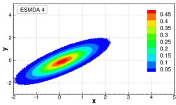
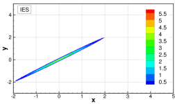
Refer to caption Refer to caption
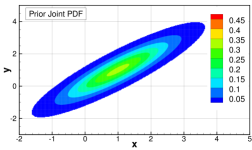
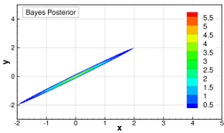
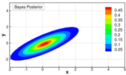
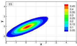
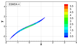
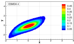
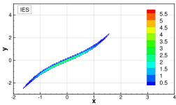
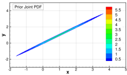
Figure 1: The plots show joint pdfs for the linear case. In the left column, the model error is set to zero (a small model error is retained in the final prediction for plotting purposes), while in the right column, we include a model error with standard deviation equal to 0.5. The two upper rows are the analytical prior and posterior, while the three lower rows show the results from ES, ESMDA with four steps, and IES.
Refer to caption Refer to caption
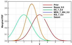
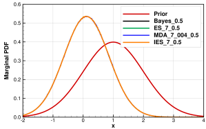
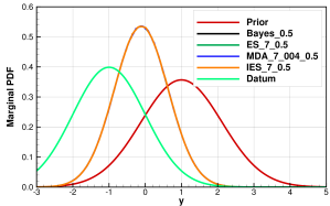
Figure 2: The plots show the marginal pdfs for x in the left column and the marginal pdfs for y in the right column for the linear case corresponding to FigureΒ 1. The upper row is the case with zero model error, while the lower row shows the result when we include a model error with standard deviation equal to 0.5. In all the plots, the legends, e.g., MDA_​7​_​004​_​0.5_7_004_0.5\_7\_004\_0.5 denote ESMDA with 107superscript10710^{7} ensemble members, 4 MDA steps, and a model error with variance equal to 0.5. Note that, in the linear case, all the methods give results that are identical to the Bayesian posterior, and the posterior pdfs are indistinguishable.
Refer to caption
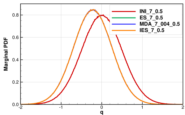
Figure 3: Model error distributions for the linear case. It is not possible to distinguish between the pdfs for the estimated model errors from the different methods.
Refer to caption Refer to caption
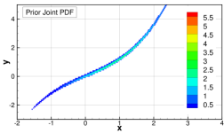
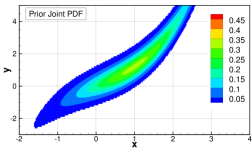
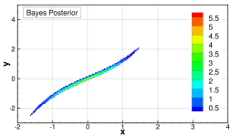
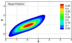
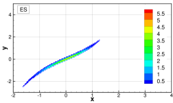
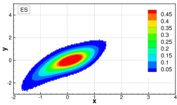
Figure 4: The plots show joint pdfs for the nonlinear case. In the left column, the model error is set to zero, while in the right column, we include a model error with standard deviation equal to 0.5. The two upper rows are the analytical prior and posterior, while the three lower rows show results from ES, ESMDA with four steps, and IES.
Refer to caption Refer to caption
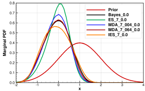
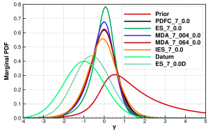
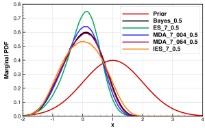
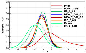
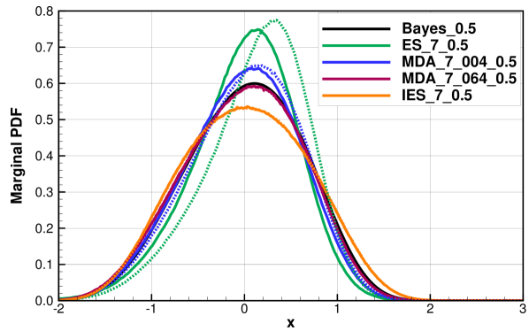
Figure 5: The plots show the marginal pdfs for xπ‘₯x in the left column and the marginal pdfs for y𝑦y in the right column for the nonlinear case corresponding to FigureΒ 4. The upper row is the case with zero model error, while the lower row shows the result when we include a model error with standard deviation equal to 0.5. In all the plots, the legends, e.g., MDA_​7​_​004​_​0.5_7_004_0.5\_7\_004\_0.5 denote ESMDA with 107superscript10710^{7} ensemble members, 4 MDA steps, and a model error with variance equal to 0.5. The legends ES_7_0.0D and ES_7_0.5D refers to an ES case where the prediction yjasuperscriptsubscript𝑦𝑗ay_{j}^{\mathrm{a}} is updated directly by Eq.Β (61).
Refer to caption
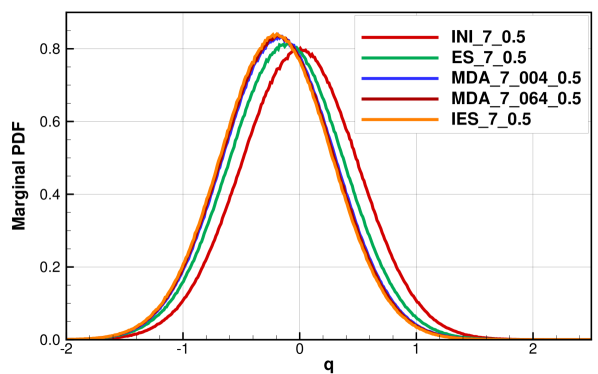
Figure 6: Model error distributions for the nonlinear case.
Refer to caption
Figure 7: The plot compares solutions including (solid lines) and excluding (dashed lines) the projection in Eq.Β (51).

6 Examples

To verify the new algorithms, we will use the scalar example from Evensen (2018). The example resembles the use of conditioning methods in history matching, i.e., there is a parameter xπ‘₯x that serves as an input to a forward model to predict y=g​(x,q)𝑦𝑔π‘₯π‘žy=g(x,q). We assume an initial state xπ‘₯x and a prediction y𝑦y, given by the model

y=g​(x,q)=x​(1+β​x2)+q.𝑦𝑔π‘₯π‘žπ‘₯1𝛽superscriptπ‘₯2π‘ž\begin{split}y&=g(x,q)\\ &=x(1+\beta x^{2})+q.\end{split} (82)

Here β𝛽\beta is a parameter that determines the nonlinearity of the model. In the current example, we have used Ξ²=0.0𝛽0.0\beta=0.0 for the linear cases and Ξ²=0.2𝛽0.2\beta=0.2 for the nonlinear cases. Clearly, in this case the model error is additive to make the linear case completely linear. If we have a product of xπ‘₯x and qπ‘žq, the problem becomes nonlinear, and we can not test if the different methods converge to the same solution in the entirely linear case where the convergence partly constitutes our proof of consistency.

The model error qπ‘žq is a random variable sampled from 𝒩​(0,Cq​q)𝒩0subscriptπΆπ‘žπ‘ž\mathcal{N}(0,C_{qq}) with Cq​q=0.0subscriptπΆπ‘žπ‘ž0.0C_{qq}=0.0 in the case with no model errors and Cq​q=0.25subscriptπΆπ‘žπ‘ž0.25C_{qq}=0.25 in the case including model errors.

In all the four cases we sample the prior ensemble for xπ‘₯x from a Gaussian distribution with mean xf=1superscriptπ‘₯f1x^{\mathrm{f}}=1 and variance Cx​x=1subscript𝐢π‘₯π‘₯1C_{xx}=1 and we sample the perturbed observations of y𝑦y from a Gaussian error distribution with mean d=βˆ’1𝑑1d=-1 and variance Cd​d=1subscript𝐢𝑑𝑑1C_{dd}=1. Thus, in the current example, xπ‘₯x represents the initial state or the model parameter, while y𝑦y is the predicted observation. The goal is to estimate xπ‘₯x given a measurement of y𝑦y and then to recompute the correct prediction of y𝑦y subject to model errors consistently with Bayes theorem.

In this example, we use a sufficiently large number of samples, i.e., 107superscript10710^{7}, to generate accurate estimates of the probability density functions and this allows us to work directly with the pdfs and to examine the converged solutions of the methods.

6.1 Results from the linear case

In Figs.Β 1 and 2 we show the results from the linear cases without and with model errors. In Fig.Β 1 we plot the joint pdfs for the prior and the updated solutions, and in Fig.Β 2 we plot the corresponding marginal pdfs.

The joint pdfs illustrate the effect of including stochastic model errors. Without model errors, there is a unique mapping from xπ‘₯x to y𝑦y, and the pdf is zero except along the curve (or line in the linear case) defined by the model function y=g​(x)𝑦𝑔π‘₯y=g(x). The prior joint pdf has a maximum value located at (x,y)=(1,1)π‘₯𝑦11(x,y)=(1,1) while the posterior joint pdf has shifted the maximum value to (x,y)=(0,0)π‘₯𝑦00(x,y)=(0,0) for all the methods. When we introduce the model errors, we notice that we obtain a stronger update in y𝑦y and weaker update in xπ‘₯x, than in the case without model errors. Still, we observe that all the smoother methods give a result that is identical to the Bayesian update. We can better visualize these results when we examine the marginal pdfs plotted in Fig.Β 2.

In the case without model errors, we see that the prediction pdf for y𝑦y and the measurement pdf have the same variance and only differ in the value of the means. The measurement is at y=βˆ’1𝑦1y=-1 while the mean prediction is located at y=1𝑦1y=1. The update from ES, ESMDA, and IES, exactly matches the Bayesian update in this case and is centered between the measurement and prediction pdf as we would expect.

When we include model errors, the effect is that the prediction gets a higher variance, although the mean is the same (in this particular case). Due to the higher variance, we give more weight to the measurement in the update and the update for y𝑦y is stronger than in the case without model errors. On the other hand, the update for xπ‘₯x is weaker in this case, since the addition of model errors reduces the correlation between the predicted measurement y𝑦y and the prior xπ‘₯x.

So, how can the update for y𝑦y be shifted towards the observation in this case? Afterall, we compute y𝑦y as a prediction from xπ‘₯x. Here the inclusion of the model errors in the inversion plays a vital role. We simultaneously update the ensemble for xπ‘₯x and the estimate of the model errors qπ‘žq. In Fig.Β 3 we see how we shift the model errors towards negative values. Thus, when we integrate the model forward from the updated xπ‘₯x, the forcing from qπ‘žq compensates for the weaker update of xπ‘₯x and also the additional shift of y𝑦y towards the measured value.

This example illustrates how model errors impact the updates of xπ‘₯x and y𝑦y as well as how we also need to include the model errors as a parameter in the estimation and then use it in the prediction to obtain the correct estimate of y𝑦y. Finally, we also demonstrate that in the linear case with and without model errors, ES, IES, and ESMDA, all converge to the correct Bayesian solution.

6.2 Results from the nonlinear case

In Figs.Β 4 and 5 we show the results from the nonlinear cases with and without model errors, where Fig.Β 4 plots the joint pdfs for the prior and the updated solutions, and in Fig.Β 5 we plot the corresponding marginal pdfs.

From the joint pdfs, we notice that the various smoother methods give different results both with and without the inclusion of model errors, although the general shape and locations of the pdfs are reasonably consistent with the theoretical solution as given by Bayes theorem.

We get a clearer picture from the marginal pdfs in Fig.Β 5. As for the linear case, we get a weaker update of xπ‘₯x and a stronger update of y𝑦y. We also notice that the introduction of model errors is handled well by the iterative methods, and the results are somewhat better and more consistent with the theoretical solution than in the case without model errors. ES is still the poorest estimator, and the iterative smoothers provide a significant improvement in the estimate, also in the case including model errors. We show the corresponding updates of the model error qπ‘žq in Fig.Β 6 and the different smoother methods all give slightly different results.

The dashed green line in the plots for y𝑦y in Fig.Β 5 is the direct ES update of y𝑦y using the predicted ensemble for y𝑦y and the measurement. It is clear that the update of xπ‘₯x followed by an integration of the model to obtain y𝑦y gives a better result than a direct update of y𝑦y. Furthermore, the additional use of iterations improves the estimate of y𝑦y even further. This result is the motivation for introducing IEnKF in sequential data assimilation (Sakov etΒ al., 2012, 2018) and also the iterative smoother by Bocquet and Sakov (2013, 2014). In history matching, we are primarely interested in estimating 𝐱𝐱{\mathbf{x}}, and the prediction 𝐲𝐲{\mathbf{y}} is just the result given the model parameters in 𝐱𝐱{\mathbf{x}}. But also in history matching, the ultimate value comes from accurate predictions of 𝐲𝐲{\mathbf{y}}.

The impact of using Eq.Β (51) for evaluating 𝐂~y​ysubscript~𝐂𝑦𝑦\widetilde{{\mathbf{C}}}_{yy} in the update schemes is illustrated in Fig.Β 7 where we show results including and excluding the projection. The impact is most pronounced when using ES and ESMDA with few update steps where the use of 𝐂¯y​ysubscript¯𝐂𝑦𝑦\overline{{\mathbf{C}}}_{yy} instead of 𝐂~y​ysubscript~𝐂𝑦𝑦\widetilde{{\mathbf{C}}}_{yy} severely impacts the computation of the long linear update steps. In IES we must include the projection to ensure that the gradients defined in Eqs.Β (77) and (81) are identical but in the current case the relative difference in the estimated mean when including or excluding the projection is only around one percent.

7 Including model errors in history matching

The need for including model errors in iterative ensemble smoothers became apparent while working with the paper (Evensen and Eikrem, 2018), which considered the conditioning of reservoir models on production-rate data. Typically, in history matching, we assign errors to the rate data used in the conditioning step, while we neglect these errors when the same data are used to force the reservoir simulation model during the historical simulation.

The errors in rate data are considered as the dominant model errors in a reservoir simulation model when we exclude errors in the model parameters that we estimate during the history matching. Also, Evensen and Eikrem (2018) pointed out that there are strong time correlations in the errors in rate data due to the rate allocation procedure used. When we include a stochastic model forcing using time-correlated errors, we will experience a significantly stronger impact than when the errors are white in time (see Chap.Β 12 in Evensen, 2009b).

The functional form 𝐲=𝐠​(𝐱,πͺ)𝐲𝐠𝐱πͺ{\mathbf{y}}={\mathbf{g}}({\mathbf{x}},{\mathbf{q}}) can represent the prediction of the produced rates (that we observe) from a reservoir simulation model. Note that using ensemble methods, we do not need to explicitly construct the functional form 𝐲=𝐠​(𝐱,πͺ)𝐲𝐠𝐱πͺ{\mathbf{y}}={\mathbf{g}}({\mathbf{x}},{\mathbf{q}}) since we represent the gradients using ensemble covariances. We only need access to a numerical reservoir simulation model. The inputs 𝐱𝐱{\mathbf{x}} then contain all the uncertain parameters of the model, such as, e.g., porosity and permeability fields, various transmissibilities, and even parameters defining the reservoir structure. The model errors can be the errors in the rates used to force the model in the historical period. These errors are not additive since the model prediction depends nonlinearly on the specified rates.

If we associate the dominant model errors with the rates used to force the simulation model, then the size of the vector of model errors πͺπͺ{\mathbf{q}} is equal to the number of rate data used to force the model. A typical number of data for a well can be 12 data points per year, i.e., if we force the model using monthly reservoir-volume rates.

The prior error statistics for the rate data used to force the model should be the same as is used for the rate data in the update step. Thus, we can simulate a prior ensemble of time series with mean zero, a specified variogram in time, and a specified variance, to represent the model errors. These time series are then defining the vectors πͺjsubscriptπͺ𝑗{\mathbf{q}}_{j} of model errors for each realization. An ensemble model-error covariance 𝐂¯q​qsubscriptΒ―π‚π‘žπ‘ž\overline{{\mathbf{C}}}_{qq} is then defined by the ensemble πͺjsubscriptπͺ𝑗{\mathbf{q}}_{j}.

The conventional procedure of deriving the production rates from rate-allocation tables, which we only update in connection with separator tests, often several years apart, means that the errors in the rate data will be nearly perfectly correlated in between each separator test. Note also that the inclusion of time correlations significantly reduces the degrees of freedom in the model errors and simplifies the estimation of the model errors in the conditioning step.

The expected impact of including model errors is first a larger and more realistic spread of the prior ensemble. Second, we will obtain a weaker and more correct update of the reservoir parameters in conditioning step. Furthermore, the posterior ensemble will give a more accurate and consistent prediction at the end of the history matching period since the posterior realizations are forced by updated and improved estimated rates. Thus, we have an improved basis for making future predictions. We also expect that the information contained in the improved estimates of rates, in some cases may be used to correct for biases in the rates used in future predictions.

8 Summary

In this paper, we have given consistent formulations of iterative ensemble smoothers when we include model errors. We demonstrate the consistency by showing that the ensemble smoothers all converge to the Bayesian posterior in the linear case. The main result is that the model errors need to be treated as another set of unknown parameters and estimated in the same way as the input parameters to the model. The proposed approach allows for the inclusion of general nonlinear errors that can be both red and white in time. Thus, we can apply the methods for history matching of reservoir models forced with uncertain rate data having time-correlated errors, as well as an iterative EnKF in sequential data assimilation with general model-error terms.

We demonstrate that the inclusion of model errors leads to a weaker update of the input parameters to the model, but a stronger update of the measured model prediction. Vice verse, the negligence of model errors that should be present, will lead to a too substantial update of the model input parameters with an associated underestimated uncertainty and also a too weak update of the prediction.

Thus, the results open for a more consistent solution of the history-matching problem, given that significant model errors are neglected in all previous history-matching applications with iterative ensemble smoothers.

We also briefly discuss an inconsistency of the linearizations in the analysis scheme that appear for nonlinear operators and when the state dimension is less than the ensemble size minus one, and we show that we must include an additional projection of the predicted measurements for consistency in the derivation of the final update equations.

Acknowledgement

This work was supported by the Research Council of Norway and the companies Aker–BP, DEA, ENI, Shell, Petrobras, Equinor, and VNG, through the Petromaks–2 project DIGIRES. Also, the work has benefited from the interaction and collaborations with the Nordforsk Nordic center of excellence in data assimilation, EMBLA. In-depth discussions with Patrick Raanes regarding the linear-regression derivation have helped to improve the manuscript, and the author is also grateful for comments by Geir NΓ¦vdal and Alberto Carrassi on early versions of the manuscript. Constructive comments by three anonymous reviewers lead to the inclusion of a section on how to practically account for model errors in reservoir history matching.

References

  • Bennett (1992) Bennett, A.Β F., Inverse Methods in Physical Oceanography, 346 pp., Cambridge University Press, 1992.
  • Bocquet and Sakov (2013) Bocquet, M., and P.Β Sakov, Joint state and parameter estimation with an iterative ensemble Kalman smoother, Nonlinear Processes in Geophysics, European Geosciences Union (EGU), 20(5), 803–818, 2013.
  • Bocquet and Sakov (2014) Bocquet, M., and P.Β Sakov, An iterative ensemble Kalman smoother, Q. J. R. Meteorol. Soc., 140, 1521–1535, 2014.
  • Carrassi and Vannitsem (2016) Carrassi, A., and S.Β Vannitsem, Deterministic treatment of model error in geophysical data assimilation, in Mathematical Paradigms of Climate Science, Springer INdAM Series, vol.Β 15, edited by F.Β Ancona, P.Β Cannarsa, C.Β Jones, and A.Β Portaluri, pp. 175–213, Springer, Cham, 2016.
  • Chen and Oliver (2012) Chen, Y., and D.Β S. Oliver, Ensemble randomized maximum likelihood method as an iterative ensemble smoother, Math. Geosci., 44, 1–26, 2012.
  • Chen and Oliver (2013) Chen, Y., and D.Β S. Oliver, Levenberg-Marquardt forms of the iterative ensemble smoother for efficient history matching and uncertainty quantification, Computat Geosci, 17, 689–703, 2013.
  • Eknes and Evensen (1997) Eknes, M., and G.Β Evensen, Parameter estimation solving a weak constraint variational formulation for an Ekman model, J.Β Geophys.Β Res., 102(C6), 12,479–12,491, 1997.
  • Emerick and Reynolds (2012) Emerick, A.Β A., and A.Β C. Reynolds, History matching time-lapse seismic data using the ensemble Kalman filter with multiple data assimilations, Computat Geosci, 16(3), 639–659, 2012.
  • Emerick and Reynolds (2013) Emerick, A.Β A., and A.Β C. Reynolds, Ensemble smoother with multiple data assimilation, Computers and Geosciences, 55, 3–15, 2013.
  • Evensen (1994) Evensen, G., Sequential data assimilation with a nonlinear quasi-geostrophic model using Monte Carlo methods to forecast error statistics, J.Β Geophys.Β Res., 99(C5), 10,143–10,162, 1994.
  • Evensen (2003) Evensen, G., The ensemble Kalman filter: Theoretical formulation and practical implementation, Ocean Dynamics, 53, 343–367, 2003.
  • Evensen (2009a) Evensen, G., The ensemble Kalman filter for combined state and parameter estimation, IEEE Control Systems Magazine, 29(3), 83–104, 2009a.
  • Evensen (2009b) Evensen, G., Data Assimilation: The Ensemble Kalman Filter, 2nd ed., 320 pp., Springer, 2009b.
  • Evensen (2018) Evensen, G., Analysis of iterative ensemble smoothers for solving inverse problems, Computat Geosci, 22(3), 885–908, doi:10.1007/s10596-018-9731-y, 2018.
  • Evensen and Eikrem (2018) Evensen, G., and K.Β S. Eikrem, Strategies for conditioning reservoir models on rate data using ensemble smoothers, Computat Geosci, 22(5), 1251–1270, doi:10.1007/s10596-018-9750-8, 2018.
  • Evensen and van Leeuwen (1996) Evensen, G., and P.Β J. van Leeuwen, Assimilation of Geosat altimeter data for the Agulhas current using the ensemble Kalman filter with a quasi-geostrophic model, Mon.Β Weather Rev., 124, 85–96, 1996.
  • Harlim (2017) Harlim, J., Model error in data assimilation, in Nonlinear and Stochastic Climate Dynamics, edited by C.Β Franzke and T.Β OΒΏKane, Cambridge University Press: Cambridge, UK, also available as arXiv:1311.3579, 2017.
  • Kitanidis (1995) Kitanidis, P.Β K., Quasi-linear geostatistical therory for inversing, Water Resources Research, 31(10), 2411–2419, 1995.
  • Neal (1996) Neal, R.Β M., Sampling from multimodal distributions using tempered transitions, Statistics and Computing, 6(4), 353–366, 1996.
  • Oliver etΒ al. (1996) Oliver, D.Β S., N.Β He, and A.Β C. Reynolds, Conditioning permeability fields to pressure data, ECMOR – 5th European Conference on the Mathematics of Oil Recovery, 1996.
  • Reynolds etΒ al. (2006) Reynolds, A.Β C., M.Β Zafari, and G.Β Li, Iterative forms of the Ensemble Klman Filter, ECMOR – 10th European Conference on the Mathematics of Oil Recovery, 2006.
  • Sakov etΒ al. (2012) Sakov, P., D.Β S. Oliver, and L.Β Bertino, An iterative EnKF for strongly nonlinear systems, Mon.Β Weather Rev., 140, 1988–2004, 2012.
  • Sakov etΒ al. (2018) Sakov, P., J.-M. Haussaire, and M.Β Bocquet, An iterative ensemble Kalman filter in the presence of additive model error, Q. J. R. Meteorol. Soc., doi: 10.1002/qj.3213, 2018.
  • Stordal and Elsheikh (2015) Stordal, A., and A.Β H. Elsheikh, Iterative ensemble smoothers in the annealed importance sampling framework, Advances in Water Resources, 86, 231–239, 2015.