Bottleneck Stability for Generalized Persistence Diagrams

Abstract

In this paper, we extend bottleneck stability to the setting of one dimensional constructible persistences module valued in any skeletally small abelian category.

1 Introduction

Persistent homology is a way of quantifying the topology of a function. Given a function $f:X\to{\mathbb{R}}$, persistence scans the homology of the sublevel sets $f^{-1}(-\infty,r]$ as $r$ varies from $-\infty$ to $\infty$. As it scans, homology appears and homology disappears. This history of births and deaths is recorded as a persistence diagram [CSEH07] or a barcode [ZC05]. What makes persistence special is that the persistence diagram of $f$ is stable to arbitrary perturbations to $f$. This is the celebrated bottleneck stability of Cohen-Steiner, Edelsbrunner, and Harer [CSEH07]. Bottleneck stability makes persistent homology a useful tool in data analysis and in pure mathematics. All of this is in the setting of vector spaces where each homology group is computed using coefficients in a field.

Fix a field $\mathsf{k}$ and let ${\mathsf{Vec}}$ be the category of $\mathsf{k}$-vector spaces. As persistence scans the sublevel sets of $f$, it records its homology as a functor ${\mathsf{F}}:({\mathbb{R}},\leq)\to{\mathsf{Vec}}$ where ${\mathsf{F}}(r):={\mathsf{H}}_{\ast}\big{(}f^{-1}(-\infty,r];\mathsf{k}\big{)}$ and ${\mathsf{F}}(r\leq s):{\mathsf{F}}(r)\to{\mathsf{F}}(s)$ is the map induced by the inclusion of the sublevel set at $r$ into the sublevel set at $s$. The functor ${\mathsf{F}}$ is called the persistence module of $f$. Assuming some tameness conditions on $f$, the persistence diagram of ${\mathsf{F}}$ is equivalent to its barcode, but the two definitions are very different. The barcode of ${\mathsf{F}}$ is its list of indecomposables. This list is unique up to a permutation and furthermore, each indecomposable is an interval persistence module [ZC05, CdS10, CB15]. The barcode model is how most people now think about persistence. However in [CSEH07] where bottleneck stability was first proved, the persistence diagram is defined as a purely combinatorial object. The rank function of ${\mathsf{F}}$ assigns to each pair of values $r\leq s$ the rank of the map ${\mathsf{F}}(r\leq s)$. The Möbius inversion of the rank function is the persistence diagram of ${\mathsf{F}}$. Remarkably, these two very different approaches to persistence give equivalent answers.

The persistence diagram of [CSEH07] easily generalizes [Pat18] to the setting of constructible persistence modules valued in any skeletally small abelian category ${\mathcal{C}}$. The rank function of such a persistence module records the image of each ${\mathsf{F}}(r\leq s)$ as an element of the Grothendieck group of $\mathcal{C}$. Here we are using the Grothendieck group of an abelian category: this is the abelian group with one generator for each isomorphism class of objects and one relation for each short exact sequence. The persistence diagram of ${\mathsf{F}}$ is then the Möbius inversion of this rank function. A weak form of stability was shown in [Pat18]. In this paper, we prove bottleneck stability. Our proof is an adaptation of the proofs of [CSEH07] and [CdSGO16].

We were hoping that the Möbius inversion model for persistence would lead to a good theory of persistence for multiparameter persistence modules ${\mathsf{F}}:({\mathbb{R}}^{k},\leq)\to~{}{\mathcal{C}}$ [CZ09, Les15]. The Möbius inversion applies to arbitrary finite posets. Assuming some finiteness conditions on ${\mathsf{F}}$, we may define its persistence diagram as the Möbius inversion of its rank function. The proof of bottleneck stability presented in this paper requires positivity of the persistence diagram; see Proposition 4.6. Unfortunately, there are simple examples of multiparameter persistence modules whose persistence diagrams are not positive. Therefore the proof presented here does not generalize to the multiparameter setting. It seems that the Möbius inversion model for persistence works well only in the setting of one-parameter constructible persistence modules.

2 Persistence Modules

Fix a skeletally small abelian category $\mathcal{C}$. By skeletally small, we mean that the collection of isomorphism classes of objects in $\mathcal{C}$ is a set. For example, $\mathcal{C}$ may be the category of finite dimensional $\mathsf{k}$-vector spaces, the category of finite abelian groups, or the category of finite length $R$-modules. Let $\bar{{\mathbb{R}}}:={\mathbb{R}}\cup\{\infty\}$ be the totally ordered set of real numbers with the point $\infty$ satisfying $p<\infty$ for all $p\in{\mathbb{R}}$. For any $p\in\bar{\mathbb{R}}$, we let $\infty+p=\infty$.

Definition 2.1:

A persistence module is a functor ${\mathsf{F}}:{\mathbb{R}}\to\mathcal{C}$. Let

$$S=\{s_{1}<s_{2}<\cdots<s_{k}<\infty\}\subseteq\bar{\mathbb{R}}$$

be a finite subset. A persistence module ${\mathsf{F}}$ is $S$-constructible if it satisfies the following two conditions:

• For $p\leq q<s_{1}$, ${\mathsf{F}}(p\leq q):0\to 0$ is the zero map.

• For $s_{i}\leq p\leq q<s_{i+1}$, ${\mathsf{F}}(p\leq q)$ is an isomorphism.

• For $s_{k}\leq p\leq q\leq\infty$, ${\mathsf{F}}(p\leq q)$ is an isomorphism.

For example, let $f:M\to{\mathbb{R}}$ be a Morse function on a compact manifold $M$. The function $f$ filters $M$ by sublevel sets $M_{\leq r}^{f}:=\{p\in M\;|\;f(p)\leq r\}$. For every $r\leq s$, $M_{\leq r}^{f}\subseteq M_{\leq s}^{f}$. Now apply homology with coefficients in a finite abelian group. The result is a persistence module of finite abelian groups that is constructible with respect to the set of critical values of $f$ union $\{\infty\}$. If one applies homology with coefficients in a field $\mathsf{k}$, then the result is a constructible persistence module of finite dimensional $\mathsf{k}$-vector spaces. In topological data analysis, one usually starts with a constructible filtration of a finite simplicial complex.

There is a natural distance between persistence modules called the interleaving distance [CCSG⁺09]. For any $\varepsilon\geq 0$, let ${\mathbb{R}}\times_{\varepsilon}\{0,1\}$ to be the poset $\big{(}{\mathbb{R}}\times\{0\}\big{)}\cup\big{(}{\mathbb{R}}\times\{1\}\big{)}$ where $(p,t)\leq(q,s)$ if

• $t=s$ and $p\leq q$, or

• $t\neq s$ and $p+\varepsilon\leq q$.

Let $\iota_{0},\iota_{1}:{\mathbb{R}}\hookrightarrow{\mathbb{R}}\times_{\varepsilon}\{0,1\}$ be the poset maps $\iota_{0}:p\mapsto(p,0)$ and $\iota_{1}:p\mapsto(p,1)$.

Definition 2.2:

An $\varepsilon$-interleaving between two constructible persistence modules ${\mathsf{F}}$ and ${\mathsf{G}}$ is a functor $\Phi$ that makes the following diagram commute up to a natural isomorphism:

$$\begin{gathered}\lx@xy@svg{\hbox{\raise 0.0pt\hbox{\kern 6.68056pt\hbox{\ignorespaces\ignorespaces\ignorespaces\hbox{\vtop{\kern 0.0pt\offinterlineskip\halign{\entry@#!@&&\entry@@#!@\cr&\\&&\\&&\crcr}}}\ignorespaces{\hbox{\kern-3.0pt\raise 0.0pt\hbox{\hbox{\kern 0.0pt\raise 0.0pt\hbox{\hbox{\kern 3.0pt\raise 0.0pt\hbox{$\textstyle{}$}}}}}}}{\hbox{\kern 30.68056pt\raise 0.0pt\hbox{\hbox{\kern 0.0pt\raise 0.0pt\hbox{\hbox{\kern 3.0pt\raise 0.0pt\hbox{$\textstyle{{\mathbb{R}}\times_{\varepsilon}\{0,1\}\ignorespaces\ignorespaces\ignorespaces\ignorespaces}$}}}}}}}\ignorespaces\ignorespaces\ignorespaces{}\ignorespaces\ignorespaces{\hbox{\lx@xy@drawline@}}\ignorespaces\ignorespaces\ignorespaces{\hbox{\kern 54.77794pt\raise-37.62498pt\hbox{{}\hbox{\kern 0.0pt\raise 0.0pt\hbox{\hbox{\kern 3.0pt\hbox{\hbox{\kern 0.0pt\raise-2.39166pt\hbox{$\scriptstyle{\Phi}$}}}\kern 3.0pt}}}}}}\ignorespaces{\hbox{\kern 54.77794pt\raise-65.41666pt\hbox{\hbox{\kern 0.0pt\raise 0.0pt\hbox{\lx@xy@tip{1}\lx@xy@tip{-1}}}}}}\ignorespaces\ignorespaces{\hbox{\lx@xy@drawline@}}\ignorespaces{\hbox{\lx@xy@drawline@}}{\hbox{\kern-6.68056pt\raise-38.41666pt\hbox{\hbox{\kern 0.0pt\raise 0.0pt\hbox{\hbox{\kern 3.0pt\raise 0.0pt\hbox{$\textstyle{{\mathbb{R}}\ignorespaces\ignorespaces\ignorespaces\ignorespaces\ignorespaces\ignorespaces\ignorespaces\ignorespaces}$}}}}}}}\ignorespaces\ignorespaces\ignorespaces{\hbox{\kern 6.68056pt\raise-33.73245pt\hbox{\hbox{\kern 0.0pt\raise 0.0pt\hbox{\lx@xy@hook{1}}}}}}\ignorespaces\ignorespaces{\hbox{\lx@xy@drawline@}}\ignorespaces\ignorespaces\ignorespaces{\hbox{\kern 18.47691pt\raise-14.05695pt\hbox{{}\hbox{\kern 0.0pt\raise 0.0pt\hbox{\hbox{\kern 3.0pt\hbox{\hbox{\kern 0.0pt\raise-0.8625pt\hbox{$\scriptstyle{\iota_{0}}$}}}\kern 3.0pt}}}}}}\ignorespaces{\hbox{\kern 46.93614pt\raise-5.5pt\hbox{\hbox{\kern 0.0pt\raise 0.0pt\hbox{\lx@xy@tip{1}\lx@xy@tip{-1}}}}}}\ignorespaces\ignorespaces{\hbox{\lx@xy@drawline@}}\ignorespaces{\hbox{\lx@xy@drawline@}}\ignorespaces\ignorespaces\ignorespaces{}\ignorespaces\ignorespaces{\hbox{\lx@xy@drawline@}}\ignorespaces\ignorespaces\ignorespaces{\hbox{\kern 18.54324pt\raise-62.22498pt\hbox{{}\hbox{\kern 0.0pt\raise 0.0pt\hbox{\hbox{\kern 3.0pt\hbox{\hbox{\kern 0.0pt\raise-2.39166pt\hbox{$\scriptstyle{{\mathsf{F}}}$}}}\kern 3.0pt}}}}}}\ignorespaces{\hbox{\kern 46.77794pt\raise-69.87497pt\hbox{\hbox{\kern 0.0pt\raise 0.0pt\hbox{\lx@xy@tip{1}\lx@xy@tip{-1}}}}}}\ignorespaces\ignorespaces{\hbox{\lx@xy@drawline@}}\ignorespaces{\hbox{\lx@xy@drawline@}}{\hbox{\kern 51.77794pt\raise-38.41666pt\hbox{\hbox{\kern 0.0pt\raise 0.0pt\hbox{\hbox{\kern 3.0pt\raise 0.0pt\hbox{$\textstyle{}$}}}}}}}{\hbox{\kern 102.87532pt\raise-38.41666pt\hbox{\hbox{\kern 0.0pt\raise 0.0pt\hbox{\hbox{\kern 3.0pt\raise 0.0pt\hbox{$\textstyle{{\mathbb{R}}\ignorespaces\ignorespaces\ignorespaces\ignorespaces\ignorespaces\ignorespaces\ignorespaces\ignorespaces}$}}}}}}}\ignorespaces\ignorespaces\ignorespaces{\hbox{\kern 102.87532pt\raise-33.73897pt\hbox{\hbox{\kern 0.0pt\raise 0.0pt\hbox{\lx@xy@hook{1}}}}}}\ignorespaces\ignorespaces{\hbox{\lx@xy@drawline@}}\ignorespaces\ignorespaces\ignorespaces{\hbox{\kern 80.60143pt\raise-14.05695pt\hbox{{}\hbox{\kern 0.0pt\raise 0.0pt\hbox{\hbox{\kern 3.0pt\hbox{\hbox{\kern 0.0pt\raise-0.8625pt\hbox{$\scriptstyle{\iota_{1}}$}}}\kern 3.0pt}}}}}}\ignorespaces{\hbox{\kern 62.61436pt\raise-5.5pt\hbox{\hbox{\kern 0.0pt\raise 0.0pt\hbox{\lx@xy@tip{1}\lx@xy@tip{-1}}}}}}\ignorespaces\ignorespaces{\hbox{\lx@xy@drawline@}}\ignorespaces{\hbox{\lx@xy@drawline@}}\ignorespaces\ignorespaces\ignorespaces{}\ignorespaces\ignorespaces{\hbox{\lx@xy@drawline@}}\ignorespaces\ignorespaces\ignorespaces{\hbox{\kern 80.28134pt\raise-62.22498pt\hbox{{}\hbox{\kern 0.0pt\raise 0.0pt\hbox{\hbox{\kern 3.0pt\hbox{\hbox{\kern 0.0pt\raise-2.39166pt\hbox{$\scriptstyle{{\mathsf{G}}}$}}}\kern 3.0pt}}}}}}\ignorespaces{\hbox{\kern 62.77795pt\raise-69.86716pt\hbox{\hbox{\kern 0.0pt\raise 0.0pt\hbox{\lx@xy@tip{1}\lx@xy@tip{-1}}}}}}\ignorespaces\ignorespaces{\hbox{\lx@xy@drawline@}}\ignorespaces{\hbox{\lx@xy@drawline@}}{\hbox{\kern-3.0pt\raise-75.24997pt\hbox{\hbox{\kern 0.0pt\raise 0.0pt\hbox{\hbox{\kern 3.0pt\raise 0.0pt\hbox{$\textstyle{}$}}}}}}}{\hbox{\kern 46.77794pt\raise-75.24997pt\hbox{\hbox{\kern 0.0pt\raise 0.0pt\hbox{\hbox{\kern 3.0pt\raise 0.0pt\hbox{$\textstyle{\mathcal{C}.}$}}}}}}}{\hbox{\kern 106.55588pt\raise-75.24997pt\hbox{\hbox{\kern 0.0pt\raise 0.0pt\hbox{\hbox{\kern 3.0pt\raise 0.0pt\hbox{$\textstyle{}$}}}}}}}\ignorespaces}}}}\ignorespaces\end{gathered} \textstyle{{\mathbb{R}}\times_{\varepsilon}\{0,1\}\ignorespaces\ignorespaces\ignorespaces\ignorespaces} \scriptstyle{\Phi} \textstyle{{\mathbb{R}}\ignorespaces\ignorespaces\ignorespaces\ignorespaces\ignorespaces\ignorespaces\ignorespaces\ignorespaces} \scriptstyle{\iota_{0}} \scriptstyle{{\mathsf{F}}} \textstyle{{\mathbb{R}}\ignorespaces\ignorespaces\ignorespaces\ignorespaces\ignorespaces\ignorespaces\ignorespaces\ignorespaces} \scriptstyle{\iota_{1}} \scriptstyle{{\mathsf{G}}} \textstyle{\mathcal{C}.} \textstyle{{\mathbb{R}}\times_{\varepsilon}\{0,1\}\ignorespaces\ignorespaces\ignorespaces\ignorespaces} \scriptstyle{\Phi} \textstyle{{\mathbb{R}}\ignorespaces\ignorespaces\ignorespaces\ignorespaces\ignorespaces\ignorespaces\ignorespaces\ignorespaces} \scriptstyle{\iota_{0}} \scriptstyle{{\mathsf{F}}} \textstyle{{\mathbb{R}}\ignorespaces\ignorespaces\ignorespaces\ignorespaces\ignorespaces\ignorespaces\ignorespaces\ignorespaces} \scriptstyle{\iota_{1}} \scriptstyle{{\mathsf{G}}} \textstyle{\mathcal{C}.}$$ (1)

Two constructible persistence modules ${\mathsf{F}}$ and ${\mathsf{G}}$ are $\varepsilon$-interleaved if there is an $\varepsilon$-interleaving between them. The interleaving distance $d_{I}({\mathsf{F}},{\mathsf{G}})$ between ${\mathsf{F}}$ and ${\mathsf{G}}$ is the infimum over all $\varepsilon\geq 0$ such that ${\mathsf{F}}$ and ${\mathsf{G}}$ are $\varepsilon$-interleaved. This infimum is attained since both ${\mathsf{F}}$ and ${\mathsf{G}}$ are constructible. If ${\mathsf{F}}$ and ${\mathsf{G}}$ are not interleaved, then we let $d_{I}({\mathsf{F}},{\mathsf{G}})=\infty$.

Proposition 2.3 (Interpolation):

Let ${\mathsf{F}}$ and ${\mathsf{G}}$ be two $\varepsilon$-interleaved constructible persistence modules. Then there exists a one-parameter family of constructible persistence modules $\{{\mathsf{K}}_{t}\}_{t\in[0,1]}$ such that ${\mathsf{K}}_{0}\cong{\mathsf{F}}$, ${\mathsf{K}}_{1}\cong{\mathsf{G}}$, and $d_{I}({\mathsf{K}}_{t},{\mathsf{K}}_{s})\leq\varepsilon|t-s|$.

Proof.

Let ${\mathsf{F}}$ and ${\mathsf{G}}$ be $\varepsilon$-interleaved by $\Phi$ as in Definition 2.2. Define ${\mathbb{R}}\times_{\varepsilon}[0,1]$ as the poset with the underlying set ${\mathbb{R}}\times[0,1]$ and $(p,t)\leq(q,s)$ whenever $p+\varepsilon|t-s|\leq q$. Note that ${\mathbb{R}}\times_{\varepsilon}\{0,1\}$ naturally embeds into ${\mathbb{R}}\times_{\varepsilon}[0,1]$ via $\iota:(p,t)\mapsto(p,t)$. See Figure 1. Finding $\{{\mathsf{K}}_{t}\}_{t\in[0,1]}$ is equivalent to finding a functor $\Psi$ that makes the following diagram commute up to a natural isomorphism:

This functor $\Psi$ is the right Kan extension of $\Phi$ along $\iota$ for which we now give an explicit construction. For convenience, let ${\mathsf{P}}:={\mathbb{R}}\times_{\varepsilon}\{0,1\}$ and ${\mathsf{Q}}:={\mathbb{R}}\times_{\varepsilon}[0,1]$. For $(p,t)\in{\mathsf{Q}}$, let ${\mathsf{P}}\uparrow(p,t)$ be the subposet of ${\mathsf{P}}$ consisting of all elements $(p^{\prime},t^{\prime})\in{\mathsf{P}}$ such that $(p,t)\leq(p^{\prime},t^{\prime})$. The poset ${\mathsf{P}}\uparrow(p,t)$, for any $p\in{\mathbb{R}}$ and $t\notin\{0,1\}$, has two minimal elements: $(p+\varepsilon t,0)$ and $\big{(}p+\varepsilon(1-t),1\big{)}$.

Figure 1: An illustration of the poset relation on ${\mathbb{R}}\times_{\varepsilon}[0,1]$.

For $t\in\{0,1\}$, the poset ${\mathsf{P}}\uparrow(p,t)$ has one minimal element, namely $(p,t)$. Let $\Psi\big{(}(p,t)\big{)}:=\lim\Phi|_{{\mathsf{P}}\uparrow(p,t)}$. For $(p,t)\leq(q,s)$, the poset ${\mathsf{P}}\uparrow(q,s)$ is a subposet of ${\mathsf{P}}\uparrow(p,t)$. This subposet relation allows us to define the morphism $\Psi\big{(}(p,t)\leq(q,s)\big{)}$ as the universal morphism between the two limits. Note that $\Psi\big{(}(p,0)\big{)}$ is isomorphic to ${\mathsf{F}}(p)$ and $\Psi\big{(}(p,1)\big{)}$ is isomorphic to ${\mathsf{G}}(p)$.

We now argue that each persistence module ${\mathsf{K}}_{t}:=\Psi(\cdot,t)$ is constructible. As we increase $p$ while keeping $t$ fixed, the limit ${\mathsf{K}}_{t}(p)$ changes only when one of the two minimal objects of ${\mathsf{P}}\uparrow(p,t)$ changes isomorphism type. Since ${\mathsf{F}}$ and ${\mathsf{G}}$ are constructible, there are only finitely many such changes to the isomorphism type of ${\mathsf{K}}_{t}(p)$. ∎

3 Persistence Diagrams

Fix an abelian group ${\mathcal{G}}$ with a translation invariant partial ordering $\preceq$. That is for all $a,b,c\in{\mathcal{G}}$, if $a\leq b$, then $a+c\leq b+c$. Roughly speaking, a persistence diagram is the assignment to each interval of the real line an element of ${\mathcal{G}}$. In our setting, only finitely many intervals will have a nonzero value.

Definition 3.1:

Let ${\mathsf{Dgm}}$ be the poset of intervals consisting of the following data:

• The objects of ${\mathsf{Dgm}}$ are intervals $[p,q)\subseteq\bar{\mathbb{R}}$ where $p\leq q$.

• The ordering is inclusion $[p_{2},q_{2})\subseteq[p_{1},q_{1})$.

Given a finite set $S=\{s_{1}<s_{2}<\cdots<s_{k}<\infty\}\subseteq\bar{{\mathbb{R}}}$, we use ${\mathsf{Dgm}}(S)$ to denote the subposet of ${\mathsf{Dgm}}$ consisting of all intervals $[p,q)$ with $p,q\in S$. The diagonal $\Delta\subseteq{\mathsf{Dgm}}$ is the subset of intervals of the form $[p,p)$. See Figure 2.

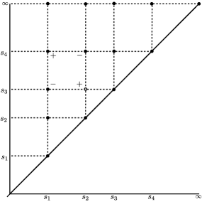
Figure 2: An interval $I=[p,q)$ is visualized as the point $(p,q)$ in the plane. The poset ${\mathsf{Dgm}}$ is therefore the set of points in the plane on and above the diagonal. In this example, $S=\{s_{1}<s_{2}<s_{3}<s_{4}<\infty\}$ and ${\mathsf{Dgm}}(S)$ is its set of grid points. Given an $S$-constructible persistence module ${\mathsf{F}}$ and an interval $[s_{2},s_{3})$, $\tilde{{\mathsf{F}}}\big{(}[s_{2},s_{3})\big{)}=d{\mathsf{F}}\big{(}[s_{2},s_{3})\big{)}-d{\mathsf{F}}\big{(}[s_{2},s_{4})\big{)}+d{\mathsf{F}}\big{(}[s_{1},s_{4})\big{)}-d{\mathsf{F}}\big{(}[s_{1},s_{3})\big{)}$.

Definition 3.2:

A persistence diagram is a map $Y:{\mathsf{Dgm}}\to{\mathcal{G}}$ with finite support. That is, there are only finitely many intervals $I\in{\mathsf{Dgm}}$ such that $Y(I)\neq 0$.

We now introduce the bottleneck distance between persistence diagrams.

Definition 3.3:

A matching between two persistence diagrams $Y_{1},Y_{2}:{\mathsf{Dgm}}\to{\mathcal{G}}$ is a map $\gamma:{\mathsf{Dgm}}\times{\mathsf{Dgm}}\to{\mathcal{G}}$ satisfying

$$Y_{1}(I) =\sum_{J\in{\mathsf{Dgm}}}\gamma(I,J)\textrm{ for all }I\in{\mathsf{Dgm}}\backslash\Delta$$

$$Y_{2}(J) =\sum_{I\in{\mathsf{Dgm}}}\gamma(I,J)\textrm{ for all }J\in{\mathsf{Dgm}}\backslash\Delta.$$

The norm of a matching $\gamma$ is

$$||\gamma||:=\max_{\big{\{}I=[p_{1},q_{1}),J=[p_{2},q_{2})\,\big{|}\,\gamma(I,J)\neq 0\big{\}}}\big{\{}|p_{1}-p_{2}|,|q_{1}-q_{2}|\big{\}}.$$

If either $q_{1}$ or $q_{2}$ is $\infty$, then $|q_{1}-q_{2}|=\infty$. The bottleneck distance between two persistence diagrams $Y_{1},Y_{2}:{\mathsf{Dgm}}\to{\mathcal{G}}$ is

$$d_{B}(Y_{1},Y_{2}):=\inf_{\gamma}||\gamma||$$

over all matchings $\gamma$ between $Y_{1}$ and $Y_{2}$. This infimum is attained since persistence diagrams have finite support.

4 Diagram of a Module

We now describe the construction of a persistence diagram from a constructible persistence module. Fix a skeletally small abelian category ${\mathcal{C}}$.

Definition 4.1:

The Grothendieck group ${\mathcal{G}}(\mathcal{C})$ of $\mathcal{C}$ is the abelian group with one generator for each isomorphism class $[a]$ of objects $a\in\mathsf{ob}\;\mathcal{C}$ and one relation $[b]=[a]+[c]$ for each short exact sequence $0\to a\to b\to c\to 0.$ The Grothendieck group has a natural translation invariant partial ordering where $[a]\preceq[b]$ whenever $a\hookrightarrow b$. For each $a\hookrightarrow b$, we have $a\oplus c\hookrightarrow b\oplus c$ for any object $c$ in $\mathcal{C}$. This makes $\preceq$ a translation invariant partial ordering.

Example 4.2:

Here are three examples of $\mathcal{C}$ with their Grothendieck groups.

• Let ${\mathsf{Vec}}$ be the category of finite dimensional $\mathsf{k}$-vector spaces for some fixed field $\mathsf{k}$. The isomorphism class of a finite dimensional $\mathsf{k}$-vector space is completely determined by its dimension. This means that the free abelian group generated by the set of isomorphism classes in ${\mathsf{Vec}}$ is $\bigoplus_{n}{\mathbb{Z}}$ where $n\geq 0$ is a natural number. Since every short exact sequence in ${\mathsf{Vec}}$ splits, the only relations are of the form $[A]+[B]=[C]$ whenever $A\oplus B\cong C$. Therefore ${\mathcal{G}}({\mathsf{Vec}})\cong{\mathbb{Z}}$ where the translation invariant partial ordering $\preceq$ is the usual total ordering on the integers.

• Let ${\mathsf{FinAb}}$ be the category of finite abelian groups. A finite abelian group is isomorphic to

  $$\dfrac{{\mathbb{Z}}}{p_{1}^{n_{1}}{\mathbb{Z}}}\oplus\cdots\oplus\dfrac{{\mathbb{Z}}}{p_{k}^{n_{k}}{\mathbb{Z}}}$$

  where each $p_{i}$ is prime. The free abelian group generated by the set of isomorphism classes in ${\mathsf{FinAb}}$ is $\bigoplus_{(p,n)}{\mathbb{Z}}$ over all pairs $(p,n)$ where $p$ is prime and $n\geq 0$ a natural number. Every primary cyclic group $\dfrac{{\mathbb{Z}}}{p^{n}{\mathbb{Z}}}$ fits into a short exact sequence

  giving rise to a relation $\left[\dfrac{{\mathbb{Z}}}{p^{n}{\mathbb{Z}}}\right]=\left[\dfrac{{\mathbb{Z}}}{p^{n-1}{\mathbb{Z}}}\right]+\left[\dfrac{{\mathbb{Z}}}{p{\mathbb{Z}}}\right].$ By induction, $\left[\dfrac{{\mathbb{Z}}}{p^{n}{\mathbb{Z}}}\right]=n\left[\dfrac{{\mathbb{Z}}}{p{\mathbb{Z}}}\right]$. Therefore ${\mathcal{G}}({\mathsf{FinAb}})\cong\bigoplus_{p}{\mathbb{Z}}$ where $p$ is prime. For two elements $[a],[b]\in{\mathcal{G}}({\mathsf{FinAb}})$, $[a]\preceq[b]$ if the multiplicity of each prime factor of $[a]$ is at most the multiplicity of each prime factor of $[b]$.

• Let ${\mathsf{Ab}}$ be the category of finitely generated abelian groups. A finitely generated abelian group is isomorphic to

  $${\mathbb{Z}}^{m}\oplus\dfrac{{\mathbb{Z}}}{p_{1}^{n_{1}}{\mathbb{Z}}}\oplus\cdots\oplus\dfrac{{\mathbb{Z}}}{p_{k}^{n_{k}}{\mathbb{Z}}}$$

  where each $p_{i}$ is prime. The free abelian group generated by the set of isomorphism classes in ${\mathsf{Ab}}$ is ${\mathbb{Z}}\oplus\bigoplus_{(p,n)}{\mathbb{Z}}$ over all pairs $(p,n)$ where $p$ is prime and $n\geq 0$ a natural number. In addition to the short exact sequences in ${\mathsf{FinAb}}$, we have

  giving rise to the relation $\left[\dfrac{{\mathbb{Z}}}{p{\mathbb{Z}}}\right]=[0]$. Therefore ${\mathcal{G}}({\mathsf{Ab}})\cong{\mathbb{Z}}$ where $\preceq$ is the usual total ordering on the integers. Unfortunately all torsion is lost.

Given a constructible persistence module, we now record the images of all its maps as elements of the Grothendieck group.

Definition 4.3:

Let $S=\{s_{1}<\cdots<s_{k}<\infty\}$ be a finite set and ${\mathsf{F}}$ an $S$-constructible persistence module valued in $\mathcal{C}$. Choose a $\delta>0$ such that $s_{i-1}<s_{i}-\delta$, for all $1<i\leq k$. The rank function of ${\mathsf{F}}$ is the map $d{\mathsf{F}}:{\mathsf{Dgm}}\to{\mathcal{G}}(\mathcal{C})$ defined as follows:

$$d{\mathsf{F}}(I)=\begin{cases}\big{[}\mathsf{im}\,{\mathsf{F}}(p<s_{i}-\delta)\big{]}&\text{for }I=[p,s_{i})\text{ where }1\leq i\leq k\\ \big{[}\mathsf{im}\,{\mathsf{F}}(p\leq q)\big{]}&\text{for all other }I=[p,q).\end{cases}$$

Note that for any $[p,q)\in{\mathsf{Dgm}}$, $d{\mathsf{F}}\big{(}[p,q)\big{)}$ equals $d{\mathsf{F}}(I)$ where $I$ is the largest interval in ${\mathsf{Dgm}}(S)$ containing $[p,q)$. This means that $d{\mathsf{F}}$ is uniquely determined by its value on ${\mathsf{Dgm}}(S)$.

Proposition 4.4:

Let ${\mathsf{F}}$ be a constructible persistence module valued in a skeletally small abelian category $\mathcal{C}$. Then its rank function $d{\mathsf{F}}:{\mathsf{Dgm}}\to{\mathcal{G}}(\mathcal{C})$ is a poset reversing map. That is for any pair of intervals $[p_{2},q_{2})\subseteq[p_{1},q_{1})$, $d{\mathsf{F}}\big{(}[p_{1},q_{1})\big{)}\preceq d{\mathsf{F}}\big{(}[p_{2},q_{2})\big{)}$.

Proof.

Suppose ${\mathsf{F}}$ is $S=\{s_{1}<\cdots<s_{k}<\infty\}$-constructible. Consider the following commutative diagram:

We may assume $q_{1},q_{2}\notin S$. If this is not the case, replace $q_{1}$ and/or $q_{2}$ in the above diagram with $q_{1}-\delta$ and $q_{2}-\delta$ for some sufficiently small $\delta>0$. We have $d{\mathsf{F}}\big{(}[p_{1},q_{1})\big{)}=[\mathsf{im}\,h]$ and $d{\mathsf{F}}\big{(}[p_{2},q_{2})\big{)}=[\mathsf{im}\,f]$. Let $I:=\mathsf{im}\,(f\circ e)$ and $K:=I\cap\ker g$. Then $K\hookrightarrow I\hookrightarrow\mathsf{im}\,f$ and $\mathsf{im}\,h\cong\nicefrac{{I}}{{K}}$. Therefore $d{\mathsf{F}}\big{(}[p_{1},q_{1})\big{)}\preceq d{\mathsf{F}}\big{(}[p_{2},q_{2})\big{)}$. ∎

Given the rank function $d{\mathsf{F}}:{\mathsf{Dgm}}\to{\mathcal{G}}(\mathcal{C})$ of an $S$-constructible persistence module ${\mathsf{F}}$, there is a unique map $\tilde{\mathsf{F}}:{\mathsf{Dgm}}\to{\mathcal{G}}$ such that

$$d{\mathsf{F}}(I)=\sum_{J\in{\mathsf{Dgm}}:J\supseteq I}\tilde{\mathsf{F}}(J)$$ (2)

for each $I\in{\mathsf{Dgm}}$. This equation is the Möbius inversion formula. For each $I=[s_{i},s_{j})$ in ${\mathsf{Dgm}}(S)$,

$$\tilde{\mathsf{F}}(I)=d{\mathsf{F}}\big{(}[s_{i},s_{j})\big{)}-d{\mathsf{F}}\big{(}[s_{i},s_{j+1})\big{)}+d{\mathsf{F}}\big{(}[s_{i-1},s_{j+1})\big{)}-d{\mathsf{F}}\big{(}[s_{i-1},s_{j})\big{)}.$$ (3)

For each $I=[s_{i},\infty)$ in ${\mathsf{Dgm}}(S)$,

$$\tilde{\mathsf{F}}(I)=d{\mathsf{F}}\big{(}[s_{i},\infty)\big{)}-d{\mathsf{F}}\big{(}[s_{i-1},\infty)\big{)}.$$ (4)

For all other $I\in{\mathsf{Dgm}}$, $\tilde{\mathsf{F}}(I)=0$. Here we have to be careful with our indices. It is possible $s_{j+1}$ or $s_{i-1}$ is not in $S$. If $s_{j+1}$ is not in $S$, let $s_{j+1}=\infty$. If $s_{i-1}$ is not in $S$, let $s_{i-1}$ be any value strictly less than $s_{1}$. We call $\tilde{\mathsf{F}}$ the Möbius inversion of $d{\mathsf{F}}$.

Definition 4.5:

The persistence diagram of a constructible persistence module ${\mathsf{F}}$ is the Möbius inversion $\tilde{\mathsf{F}}$ of its rank function $d{\mathsf{F}}$.

The Grothendieck group of ${\mathcal{C}}$ has one relation for each short exact sequence in ${\mathcal{C}}$. These relations ensure that the persistence diagram of a persistence module is positive which plays a key role in the proof of Lemma 5.3.

Proposition 4.6 (Positivity [Pat18]):

Let ${\mathsf{F}}$ be a constructible persistence module valued in a skeletally small abelian category ${\mathcal{C}}$. Then for any $I\in{\mathsf{Dgm}}$, we have $[0]\preceq\tilde{\mathsf{F}}(I)$.

5 Stability

We now begin the task of proving bottleneck stability. Throughout this section, persistence modules are valued in a fixed skeletally small abelian category ${\mathcal{C}}$.

Definition 5.1:

For an interval $I=[p,q)$ in ${\mathsf{Dgm}}$ and a value $\varepsilon\geq 0$, let

$$\square_{\varepsilon}I:=\big{\{}[r,s)\in{\mathsf{Dgm}}\,\big{|}\,p-\varepsilon<r\leq p+\varepsilon\text{ and }q-\varepsilon\leq s<q+\varepsilon\big{\}}$$

be the subposet of ${\mathsf{Dgm}}$ consisting of intervals $\varepsilon$-close to $I$. If $I$ is too close to the diagonal, that is if $q-\varepsilon\leq p+\varepsilon$, then we let $\square_{\varepsilon}I$ be empty. We call $\square_{\varepsilon}I$ the $\varepsilon$-box around $I$. See Figure 3. Note that if $q=\infty$, then $\square_{\varepsilon}I=\big{\{}[r,\infty)\;\big{|}\;p-\varepsilon<r\leq p+\varepsilon\big{\}}$.

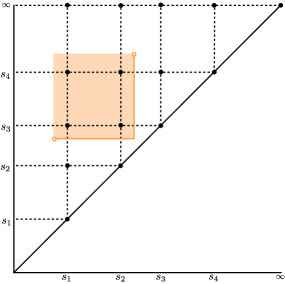
Figure 3: The shaded area is a box $\square_{\varepsilon}I$. Note that $\square_{\varepsilon}I$ is closed on the bottom and right, and it is open on the top and left.

Lemma 5.2:

Let ${\mathsf{F}}$ be an $S$-constructible persistence module, $I=[p,q)$, and $\varepsilon>0$. If $\square_{\varepsilon}I$ is nonempty, then

$$\sum_{J\in\square_{\varepsilon}I}\tilde{F}(J)=d{\mathsf{F}}\big{(}[p+\varepsilon,q-\varepsilon)\big{)}-d{\mathsf{F}}\big{(}[p+\varepsilon,q+\varepsilon)\big{)}+d{\mathsf{F}}\big{(}[p-\varepsilon,q+\varepsilon)\big{)}-d{\mathsf{F}}\big{(}[p-\varepsilon,q-\varepsilon)\big{)}$$

whenever $q\neq\infty$ and

$$\sum_{J\in\square_{\varepsilon}I}\tilde{F}(J)=d{\mathsf{F}}\big{(}[p+\varepsilon,\infty)\big{)}-d{\mathsf{F}}\big{(}[p-\varepsilon,\infty)\big{)}$$

whenever $q=\infty$.

Proof.

Both equalities follow easily from the Möbius inversion formula; see Equation 2. If $q\neq\infty$, then

$$\sum_{J\in\square_{\varepsilon}I}\tilde{\mathsf{F}}(J) =\sum_{\begin{subarray}{c}J\in{\mathsf{Dgm}}:\\ J\supseteq[p+\varepsilon,q-\varepsilon)\end{subarray}}\tilde{\mathsf{F}}(J)-\sum_{\begin{subarray}{c}J\in{\mathsf{Dgm}}:\\ J\supseteq[p+\varepsilon,q+\varepsilon)\end{subarray}}\tilde{\mathsf{F}}(J)+\sum_{\begin{subarray}{c}J\in{\mathsf{Dgm}}:\\ J\supseteq[p-\varepsilon,q+\varepsilon)\end{subarray}}\tilde{\mathsf{F}}(J)-\sum_{\begin{subarray}{c}J\in{\mathsf{Dgm}}:\\ J\supseteq[p-\varepsilon,q-\varepsilon)\end{subarray}}\tilde{\mathsf{F}}(J)$$

$$=d{\mathsf{F}}\big{(}[p+\varepsilon,q-\varepsilon)\big{)}-d{\mathsf{F}}\big{(}[p+\varepsilon,q+\varepsilon)\big{)}-d{\mathsf{F}}\big{(}[p-\varepsilon,q+\varepsilon)\big{)}+d{\mathsf{F}}\big{(}[p-\varepsilon,q-\varepsilon)\big{)}.$$

If $q=\infty$, then

$$\sum_{J\in\square_{\varepsilon}I}\tilde{\mathsf{F}}(J) =\sum_{\begin{subarray}{c}J\in{\mathsf{Dgm}}:\\ J\supseteq[p+\varepsilon,\infty)\end{subarray}}\tilde{\mathsf{F}}(J)-\sum_{\begin{subarray}{c}J\in{\mathsf{Dgm}}:\\ J\supseteq[p-\varepsilon,\infty)\end{subarray}}\tilde{\mathsf{F}}(J)$$

$$=d{\mathsf{F}}\big{(}[p+\varepsilon,\infty)\big{)}-d{\mathsf{F}}\big{(}[p-\varepsilon,\infty)\big{)}.$$

∎

Lemma 5.3 (Box Lemma):

Let ${\mathsf{F}}$ and ${\mathsf{G}}$ be two $\varepsilon$-interleaved constructible persistence modules, $I\in{\mathsf{Dgm}}$, and $\mu>0$. Then

$$\sum_{J\in\square_{\mu}I}\tilde{\mathsf{F}}(J)\preceq\sum_{J\in\square_{\mu+\varepsilon}I}\tilde{\mathsf{G}}(J)$$

whenever $\square_{\mu+\varepsilon}I$ is nonempty.

Proof.

Suppose ${\mathsf{F}}$ and ${\mathsf{G}}$ are $\varepsilon$-interleaved by $\Phi$ in Diagram 1. Define $\varphi_{r}:{\mathsf{F}}(r)\to{\mathsf{G}}(r+\varepsilon)$ as $\Phi\big{(}(r,0)\leq(r+\varepsilon,1)\big{)}$ and define $\psi_{r}:{\mathsf{G}}(r)\to{\mathsf{F}}(r+\varepsilon)$ as $\Phi\big{(}(r,1)\leq(r+\varepsilon,0)\big{)}$.

Suppose $I=[p,q)$ where $q\neq\infty$. By Lemma 5.2,

$$\sum_{J\in\square_{\mu}I}\tilde{F}(J)=\; d{\mathsf{F}}\big{(}[p+\mu,q-\mu)\big{)}-d{\mathsf{F}}\big{(}[p+\mu,q+\mu)\big{)}$$

$$+d{\mathsf{F}}\big{(}[p-\mu,q+\mu)\big{)}-d{\mathsf{F}}\big{(}[p-\mu,q-\mu)\big{)}$$

$$\sum_{J\in\square_{\mu+\varepsilon}I}\tilde{G}(J)=\; d{\mathsf{G}}\big{(}[p+\mu+\varepsilon,q-\mu-\varepsilon)\big{)}-d{\mathsf{G}}\big{(}[p+\mu+\varepsilon,q+\mu+\varepsilon)\big{)}$$

$$+d{\mathsf{G}}\big{(}[p-\mu-\varepsilon,q+\mu+\varepsilon)\big{)}-d{\mathsf{G}}\big{(}[p-\mu-\varepsilon,q-\mu-\varepsilon)\big{)}.$$

Choose a sufficiently small $\delta>0$ so that we have the following equalities:

$$d{\mathsf{F}}\big{(}[p+\mu,q-\mu)\big{)} =\big{[}\mathsf{im}\;{\mathsf{F}}(p+\mu<q-\mu-\delta)\big{]}$$

$$d{\mathsf{F}}\big{(}[p+\mu,q+\mu)\big{)} =\big{[}\mathsf{im}\;{\mathsf{F}}(p+\mu<q+\mu-\delta)\big{]}$$

$$d{\mathsf{F}}\big{(}[p-\mu,q+\mu)\big{)} =\big{[}\mathsf{im}\;{\mathsf{F}}(p-\mu<q+\mu-\delta)\big{]}$$

$$d{\mathsf{F}}\big{(}[p-\mu,q-\mu)\big{)} =\big{[}\mathsf{im}\;{\mathsf{F}}(p-\mu<q-\mu-\delta)\big{]}$$

$$d{\mathsf{G}}\big{(}[p+\mu+\varepsilon,q-\mu-\varepsilon)\big{)} =\big{[}\mathsf{im}\;{\mathsf{G}}(p+\mu+\varepsilon<q-\mu-\varepsilon-\delta)\big{]}$$

$$d{\mathsf{G}}\big{(}[p+\mu+\varepsilon,q+\mu+\varepsilon)\big{)} =\big{[}\mathsf{im}\;{\mathsf{G}}(p+\mu+\varepsilon<q+\mu+\varepsilon-\delta)\big{]}$$

$$d{\mathsf{G}}\big{(}[p-\mu-\varepsilon,q+\mu+\varepsilon)\big{)} =\big{[}\mathsf{im}\;{\mathsf{G}}(p-\mu-\varepsilon<q+\mu+\varepsilon-\delta)\big{]}$$

$$d{\mathsf{G}}\big{(}[p-\mu-\varepsilon,q-\mu-\varepsilon)\big{)} =\big{[}\mathsf{im}\;{\mathsf{F}}(p-\mu-\varepsilon<q-\mu-\varepsilon-\delta)\big{]}.$$

Consider the following commutative diagram where the horizontal and vertical arrows are the appropriate morphisms from ${\mathsf{F}}$ and ${\mathsf{G}}$:

Choose two values $a<b$ such that $a+\mu+\varepsilon<b-\mu-\varepsilon$ and let

$$T:=\{a-\mu-\varepsilon<a-\mu<a+\mu<a+\mu+\varepsilon<c<b-\mu-\varepsilon<b-\mu<b+\mu<\infty\}\subseteq\bar{\mathbb{R}}.$$

Let ${\mathsf{H}}:{\mathbb{R}}\to\mathcal{C}$ be the $T$-constructible persistence module determined by the following diagram:

Here the value of ${\mathsf{H}}$ is given on each value in $T$ and morphisms between adjacent objects are the connecting morphisms in the above commutative diagram. For example, for all $a+\mu+\varepsilon\leq r<c$, ${\mathsf{H}}(r)={\mathsf{G}}(p+\mu+\varepsilon)$ and ${\mathsf{H}}(a+\varepsilon+\mu\leq r)=\mathsf{id}$. The morphism ${\mathsf{H}}(c\leq b-\mu-\varepsilon)$ is $\psi_{q-\mu-\varepsilon-\delta}$. We have the following equalities:

$$\big{[}\mathsf{im}\;{\mathsf{F}}(p+\mu<q-\mu-\delta)\big{]} =d{\mathsf{H}}\big{(}[a+\mu,b-\mu)\big{)}$$

$$\big{[}\mathsf{im}\;{\mathsf{F}}(p+\mu<q+\mu-\delta)\big{]} =d{\mathsf{H}}\big{(}[a+\mu,b+\mu)\big{)}$$

$$\big{[}\mathsf{im}\;{\mathsf{F}}(p-\mu<q+\mu-\delta)\big{]} =d{\mathsf{H}}\big{(}[a-\mu,b+\mu)\big{)}$$

$$\big{[}\mathsf{im}\;{\mathsf{F}}(p-\mu<q-\mu-\delta)\big{]} =d{\mathsf{H}}\big{(}[a-\mu,b-\mu)\big{)}$$

$$\big{[}\mathsf{im}\;{\mathsf{G}}(p+\mu+\varepsilon<q-\mu-\varepsilon-\delta)\big{]} =d{\mathsf{H}}\big{(}[a+\mu+\varepsilon,b-\mu-\varepsilon)\big{)}$$

$$\big{[}\mathsf{im}\;{\mathsf{G}}(p+\mu+\varepsilon<q+\mu+\varepsilon-\delta)\big{]} =d{\mathsf{H}}\big{(}[a+\mu+\varepsilon,b+\mu+\varepsilon)\big{)}$$

$$\big{[}\mathsf{im}\;{\mathsf{G}}(p-\mu-\varepsilon<q+\mu+\varepsilon-\delta)\big{]} =d{\mathsf{H}}\big{(}[a-\mu-\varepsilon,b+\mu+\varepsilon)\big{)}$$

$$\big{[}\mathsf{im}\;{\mathsf{G}}(p-\mu-\varepsilon<q-\mu-\varepsilon-\delta)\big{]} =d{\mathsf{H}}\big{(}[a-\mu-\varepsilon,b-\mu-\varepsilon)\big{)}.$$

By Lemma 5.2 along with the above substitutions, we have

$$\sum_{J\in\square_{\mu}[a,b)}\tilde{\mathsf{H}}(J)=\sum_{J\in\square_{\mu}I}\tilde{{\mathsf{F}}}(J)$$

$$\sum_{J\in\square_{\mu+\varepsilon}[a,b)}\tilde{\mathsf{H}}(J)=\sum_{J\in\square_{\mu+\varepsilon}I}\tilde{G}(J).$$

By the inclusion $\square_{\mu}[a,b)\subseteq\square_{\mu+\varepsilon}[a,b)$ along with Proposition 4.6, we have

$$\sum_{J\in\square_{\mu}[a,b)}\tilde{\mathsf{H}}(J)\preceq\sum_{J\in\square_{\mu+\varepsilon}[a,b)}\tilde{\mathsf{H}}(J).$$

This proves the statement.

Suppose $I=[p,\infty)$ and let $z\in{\mathbb{R}}$ be larger than $\mu+\varepsilon$ and $s_{k}$ where ${\mathsf{F}}$ and ${\mathsf{G}}$ are $\{s_{1}<\cdots<s_{k}<\infty\}$-constructible. By Lemma 5.2,

$$\sum_{J\in\square_{\mu}I}\tilde{F}(J)=\; d{\mathsf{F}}\big{(}[p+\mu,\infty)\big{)}-d{\mathsf{F}}\big{(}[p-\mu,\infty)\big{)}$$

$$\sum_{J\in\square_{\mu+\varepsilon}I}\tilde{G}(J)=\; d{\mathsf{G}}\big{(}[p+\mu+\varepsilon,\infty)\big{)}-d{\mathsf{G}}\big{(}[p-\mu-\varepsilon,\infty)\big{)}.$$

We have the following equalities:

$$d{\mathsf{F}}\big{(}[p+\mu,\infty)\big{)} =\big{[}\mathsf{im}\;{\mathsf{F}}(p+\mu<\infty)\big{]}$$

$$d{\mathsf{F}}\big{(}[p-\mu,\infty)\big{)} =\big{[}\mathsf{im}\;{\mathsf{F}}(p-\mu<\infty)\big{]}$$

$$d{\mathsf{G}}\big{(}[p+\mu+\varepsilon,\infty)\big{)} =\big{[}\mathsf{im}\;{\mathsf{G}}(p+\mu+\varepsilon<\infty)\big{]}$$

$$d{\mathsf{G}}\big{(}[p-\mu-\varepsilon,\infty)\big{)} =\big{[}\mathsf{im}\;{\mathsf{G}}(p-\mu-\varepsilon<\infty)\big{]}.$$

Consider the following commutative diagram where the vertical and horizontal arrows are the appropriate morphisms from ${\mathsf{F}}$ and ${\mathsf{G}}$:

Note that $\psi_{\infty}$ and $\varphi_{\infty}$ are isomorphisms. Let

$$T:=\{-\mu-\varepsilon<-\mu<\mu<\mu+\varepsilon<\infty\}\subseteq\bar{\mathbb{R}}.$$

Let ${\mathsf{H}}:{\mathbb{R}}\to\mathcal{C}$ be the $T$-constructible persistence module determined by the following diagram:

Here the value of ${\mathsf{H}}$ is given on each value in $T$ and morphisms between adjacent objects are the connecting morphisms in the above commutative diagram. We have the following equalities:

$$\big{[}\mathsf{im}\;{\mathsf{F}}(p+\mu<\infty)\big{]} =d{\mathsf{H}}\big{(}[\mu,\infty)\big{)}$$

$$\big{[}\mathsf{im}\;{\mathsf{F}}(p-\mu<\infty)\big{]} =d{\mathsf{H}}\big{(}[-\mu,\infty)\big{)}$$

$$\big{[}\mathsf{im}\;{\mathsf{G}}(p+\mu+\varepsilon<\infty)\big{]} =d{\mathsf{H}}\big{(}[\mu+\varepsilon,\infty)\big{)}$$

$$\big{[}\mathsf{im}\;{\mathsf{G}}(p-\mu-\varepsilon<\infty)\big{]} =d{\mathsf{H}}\big{(}[-\mu-\varepsilon,\infty)\big{)}.$$

By Lemma 5.2 along with the above substitutions, we have

$$\sum_{J\in\square_{\mu}[0,\infty)}\tilde{\mathsf{H}}(J)=\sum_{J\in\square_{\mu}I}\tilde{{\mathsf{F}}}(J)$$

$$\sum_{J\in\square_{\mu+\varepsilon}[0,\infty)}\tilde{\mathsf{H}}(J)=\sum_{J\in\square_{\mu+\varepsilon}I}\tilde{G}(J).$$

By the inclusion $\square_{\mu}[0,\infty)\subseteq\square_{\mu+\varepsilon}[0,\infty)$ along with Proposition 4.6, we have

$$\sum_{J\in\square_{\mu}[0,\infty)}\tilde{\mathsf{H}}(J)\preceq\sum_{J\in\square_{\mu+\varepsilon}[0,\infty)}\tilde{\mathsf{H}}(J).$$

This proves the statement.

∎

Definition 5.4:

The injectivity radius of a finite set $S=\{s_{1}<s_{2}<\cdots<s_{k}<\infty\}$ is

$$\rho:=\min_{1<i\leq k}\frac{s_{i}-s_{i-1}}{2}.$$

Note that if a persistence module ${\mathsf{F}}$ is $S$-constructible and $I\in{\mathsf{Dgm}}(S)$, then

$$\tilde{\mathsf{F}}(I)=\sum_{J\in\square_{\rho}I}\tilde{\mathsf{F}}(J).$$

Lemma 5.5 (Easy Bijection):

Let ${\mathsf{F}}$ be an $S$-constructible persistence module and $\rho>0$ the injectivity radius of $S$. If ${\mathsf{G}}$ is a second constructible persistence module such that $d_{I}({\mathsf{F}},{\mathsf{G}})<\rho/2$, then $d_{B}(\tilde{\mathsf{F}},\tilde{\mathsf{G}})\leq d_{I}({\mathsf{F}},{\mathsf{G}})$.

Proof.

Let $\varepsilon=d_{I}({\mathsf{F}},{\mathsf{G}})$. Choose a sufficiently small $\mu>0$ such that $\mu+2\varepsilon<\rho$. We construct a matching $\gamma_{\mu}:{\mathsf{Dgm}}\times{\mathsf{Dgm}}\to{\mathcal{G}}({\mathcal{C}})$ such that

$$\tilde{\mathsf{F}}(I) =\sum_{J\in{\mathsf{Dgm}}}\gamma_{\mu}(I,J)\textrm{ for all }I\in{\mathsf{Dgm}}\backslash\Delta$$ (5)

$$\tilde{\mathsf{G}}(J) =\sum_{I\in{\mathsf{Dgm}}}\gamma_{\mu}(I,J)\textrm{ for all }J\in{\mathsf{Dgm}}\backslash\Delta.$$ (6)

Fix an $I\in{\mathsf{Dgm}}(S)$. By Lemma 5.3,

$$\tilde{\mathsf{F}}(I)=\sum_{J\in\square_{\mu}I}\tilde{\mathsf{F}}(I)\leq\sum_{J\in\square_{\mu+\varepsilon}I}\tilde{\mathsf{G}}(J)\leq\sum_{J\in\square_{\mu+2\varepsilon}I}\tilde{\mathsf{F}}(J)=\tilde{\mathsf{F}}(I).$$

Let $\gamma_{\mu}(I,J):=\tilde{\mathsf{G}}(J)$ for all $J\in\square_{\mu+\varepsilon}(I)$. Repeat for all $I\in{\mathsf{Dgm}}(S)$. Equation 5 is satisfied. We now check that $\gamma_{\mu}$ satisfies Equation 6. Fix an interval $J=[p,q)$ and suppose $\tilde{\mathsf{G}}(J)\neq 0$. If $q-p>\varepsilon$, then by Lemma 5.3

$$\tilde{\mathsf{G}}(J)=\sum_{I\in\square_{\mu}J}\tilde{\mathsf{G}}(I)\preceq\sum_{I\in\square_{\mu+\varepsilon}J}\tilde{\mathsf{F}}(J).$$

This means $\gamma_{\mu}(I,J)\neq 0$ for some $I\in\square_{\mu+\varepsilon}J$. If $q-p\leq\varepsilon$, then we match $J$ to the diagonal. That is, we let $\gamma_{\mu}\big{(}[\nicefrac{{q-p}}{{2}},\nicefrac{{q-p}}{{2}}),J\big{)}:=\tilde{\mathsf{G}}(J)$.

By construction, $||\gamma_{\mu}||\leq\mu+\varepsilon$ for all $\mu>0$ sufficiently small. Therefore $d_{B}(\tilde{\mathsf{F}},\tilde{\mathsf{G}})\leq\varepsilon=d_{I}(\tilde{\mathsf{F}},\tilde{\mathsf{G}})$. ∎

We are now ready to prove our main result.

Theorem 5.6 (Bottleneck Stability):

Let $\mathcal{C}$ be a skeletally small abelian category and ${\mathsf{F}},{\mathsf{G}}:{\mathbb{R}}\to\mathcal{C}$ two constructible persistence modules. Then $d_{B}\big{(}\tilde{\mathsf{F}},\tilde{\mathsf{G}}\big{)}\leq d_{I}({\mathsf{F}},{\mathsf{G}})$ where $\tilde{\mathsf{F}}$ and $\tilde{\mathsf{G}}$ are the persistence diagrams of ${\mathsf{F}}$ and ${\mathsf{G}}$, respectively.

Proof.

Let $\varepsilon=d_{I}({\mathsf{F}},{\mathsf{G}})$. By Proposition 2.3, there is a one parameter family of constructible persistence modules $\{{\mathsf{K}}_{t}\}_{t\in[0,1]}$ such that $d_{I}({\mathsf{K}}_{t},{\mathsf{K}}_{s})\leq\varepsilon|t-s|$, ${\mathsf{K}}_{0}\cong{\mathsf{F}}$, and ${\mathsf{K}}_{1}\cong{\mathsf{G}}$. Each ${\mathsf{K}}_{t}$ is constructible with respect to some set $S_{t}$, and each set $S_{t}$ has an injectivity radius $\rho_{t}>0$. For each time $t\in[0,1]$, consider the open interval

$$U(t)=(t-\nicefrac{{\rho_{t}}}{{4\varepsilon}},t+\nicefrac{{\rho_{t}}}{{4\varepsilon}})\cap[0,1]$$

By compactness of $[0,1]$, there is a finite set $Q=\{0=t_{0}<t_{1}<\cdots<t_{n}=1\}$ such that $\cup_{i=0}^{n}U(t_{i})=[0,1]$. We assume that $Q$ is minimal, that is, there does not exists a pair $t_{i},t_{j}\in Q$ such that $U(t_{i})\subseteq U(t_{j})$. If this is not the case, simply throw away $U(t_{i})$ and we still have a covering of $[0,1]$. As a consequence, for any consecutive pair $t_{i}<t_{i+1}$, we have $U(t_{i})\cap U(t_{i+1})\neq\emptyset$. This means

$$t_{i+1}-t_{i}\leq\frac{1}{4\varepsilon}(\rho_{t_{i+1}}+\rho_{t_{i}})\leq\frac{1}{2\varepsilon}\max\{\rho_{t_{i+1}},\rho_{t_{i}}\}$$

and therefore $d_{I}({\mathsf{K}}_{t_{i}},{\mathsf{K}}_{t_{i+1}})\leq\frac{1}{2}\max\{\rho_{t_{i}},\rho_{t_{i+1}}\}$. By Lemma 5.5,

$$d_{B}\big{(}\tilde{\mathsf{K}}_{t_{i}},\tilde{\mathsf{K}}_{t_{i+1}}\big{)}\leq d_{I}\big{(}{\mathsf{K}}_{t_{i}},{\mathsf{K}}_{t_{i+1}}),$$

for all $1\leq i\leq n-1$. Therefore

$$d_{B}(\tilde{\mathsf{F}},\tilde{\mathsf{G}}\big{)}\leq\sum_{i=0}^{n-1}d_{B}\big{(}\tilde{\mathsf{K}}_{t_{i}},\tilde{\mathsf{K}}_{t_{i+1}}\big{)}\leq\sum_{i=0}^{n-1}d_{I}\big{(}{\mathsf{K}}_{t_{i}},{\mathsf{K}}_{t_{i+1}})\leq\varepsilon.$$

∎

References

- [CB15] William Crawley-Boevey. Decomposition of pointwise finite-dimensional persistence modules. Journal of Algebra and Its Applications, 14(5), 2015.
- [CCSG+09] Frédéric Chazal, David Cohen-Steiner, Marc Glisse, Leonidas Guibas, and Steve Oudot. Proximity of persistence modules and their diagrams. In Proceedings of the Twenty-fifth Annual Symposium on Computational Geometry, SCG ’09, pages 237–246, New York, NY, USA, 2009. ACM.
- [CdS10] Gunnar Carlsson and Vin de Silva. Zigzag persistence. Foundations of Computational Mathematics, 10(4):367–405, 2010.
- [CdSGO16] Frédéric Chazal, Vin de Silva, Marc Glisse, and Steve Oudot. The structure and stability of persistence modules. Springer International Publishing, 2016.
- [CSEH07] David Cohen-Steiner, Herbert Edelsbrunner, and John Harer. Stability of persistence diagrams. Discrete & Computational Geometry, 37(1):103–120, 2007.
- [CZ09] Gunnar Carlsson and Afra Zomorodian. The theory of multidimensional persistence. Discrete & Computational Geometry, 42(1):71–93, Jul 2009.
- [Les15] Michael Lesnick. The theory of the interleaving distance on multidimensional persistence modules. Foundations of Computational Mathematics, 15(3):613–650, Jun 2015.
- [Pat18] Amit Patel. Generalized persistence diagrams. Journal of Applied and Computational Topology, May 2018.
- [ZC05] Afra Zomorodian and Gunnar Carlsson. Computing persistent homology. Discrete & Computational Geometry, 33(2):249–274, 2005.