Numerically computing QCD Laplace sum-rules using pySecDec

Abstract

pySecDec is a program that numerically calculates dimensionally regularized integrals. We use pySecDec to compute QCD Laplace sum-rules for pseudoscalar (i.e., $J^{PC}=0^{-+}$) charmonium hybrids, and compare the results to sum-rules computed using analytic results for dimensionally regularized integrals. We find that the errors due to the use of numerical integration methods are negligible compared to the uncertainties in the sum-rules stemming from the uncertainties in the parameters of QCD, e.g., the coupling constant, quark masses, and condensate values. Also, we demonstrate that numerical integration methods can be used to calculate finite-energy and Gaussian sum-rules in addition to Laplace sum-rules.

1 Introduction

QCD sum-rules are a well-established technique for predicting hadron properties from the QCD Lagrangian [1, 2, 3, 4]. QCD sum-rules are transformed dispersion relations that relate a correlation function of two local currents to the correlation function’s own imaginary part. The correlator is computed within the operator product expansion (OPE) in which perturbation theory is supplemented by nonperturbative corrections, each correction being a product of a perturbatively computed Wilson coefficient and a nonzero vacuum expectation value of a local operator, i.e., a condensate [5]. The imaginary part of the correlator, the hadronic spectral function, is expressed in terms of hadron properties and a continuum threshold. Hence, QCD sum-rules relate parameters of QCD (e.g., the strong coupling, quark masses, and condensates) to parameters of hadronic physics (e.g., masses, widths, and hadronic couplings) in a quantitative expression of quark-hadron duality.

When computing Wilson coefficients (including perturbation theory), we usually encounter divergent loop integrals. Such integrals are often handled using dimensional regularization. If the integrals come from Feynman diagrams with small numbers of loops, external lines, and/or distinct masses, then analytic expressions for them can often be calculated or found in the literature (e.g., [6, 7, 8, 9]). But, as the complexity of Feynman diagrams increases, computing closed-form analytic expressions for the needed dimensionally regularized integrals can become prohibitively difficult, effectively limiting the applicability of the QCD sum-rules methodology.

pySecDec is an open source Python and C++ program (which makes use of FORM [10, 11, 12], GSL [13], and the CUBA library [14, 15]) that numerically calculates dimensionally regularized integrals [16]. pySecDec has a number of features that make it attractive for use in QCD sum-rules analyses. In principle, it places no restrictions on numbers of loops, external lines, or distinct masses. Also, external momenta can take on any values in the complex plane. pySecDec computes divergent and finite parts of an integral and reports uncertainties for each. Furthermore, it can be applied to both scalar and tensor integrands.

In this article, we show that pySecDec can be successfully incorporated into the QCD sum-rules methodology. We do so by considering the two-point pseudoscalar (i.e., $J^{PC}=0^{-+}$) charmonium hybrid correlation function. This correlator and its corresponding QCD Laplace sum-rules (LSRs) were computed in [17, 18]; there, all dimensionally regularized integrals were computed analytically. Here, instead, we use pySecDec to numerically compute the needed divergent integrals, and then formulate the sum-rules with a straightforward numerical contour integral in the complex plane. We find that the errors introduced into the LSRs from numerical integration techniques are negligible compared to the uncertainties already present due to experimental uncertainties in the parameters of QCD (e.g., the strong coupling, the quark masses, and the condensates). Also, we show that numerical integration methods can be applied successfully to the computation of finite-energy sum-rules (FESRs) and Gaussian sum-rules (GSRs) in addition to LSRs.

2 Laplace sum-rules

To probe pseudoscalar charmonium hybrids, we use the current [17]

$$j_{\mu}=\frac{g_{s}}{2}\overline{c}\gamma^{\rho}\lambda^{a}\tilde{G}^{a}_{\mu\rho}c$$ (1)

where $c$ is a charm quark field and

$$\tilde{G}^{a}_{\mu\rho}=\frac{1}{2}\epsilon_{\mu\rho\omega\eta}G^{a}_{\omega\eta}$$ (2)

is the dual gluon field strength tensor defined using the Levi-Civita symbol $\epsilon_{\mu\rho\omega\eta}$. The diagonal correlator of (1) is defined and decomposed as follows:

$$\Pi_{\mu\nu}(q) =i\int\!\mathrm{d}^{4}x\,e^{iq\cdot x}\langle\Omega|\tau j_{\mu}(x)j_{\nu}^{\dagger}(0)|\Omega\rangle$$ (3)

$$=\frac{q_{\mu}q_{\nu}}{q^{2}}\Pi_{0}(q^{2})+\bigg{(}\frac{q_{\mu}q_{\nu}}{q^{2}}-g_{\mu\nu}\bigg{)}\Pi_{1}(q^{2})$$ (4)

where $\Pi_{0}(q^{2})$ probes spin-0 states and $\Pi_{1}(q^{2})$ probes spin-1 states. We are interested in pseudoscalar hybrids and so we focus on $\Pi_{0}(q^{2})$ which satisfies a dispersion relation for $q^{2}<0$,

$$\Pi_{0}(q^{2})=q^{8}\int_{t_{0}}^{\infty}\!\frac{\frac{1}{\pi}\mathrm{Im}\Pi_{0}(t)}{t^{4}(t-q^{2})}\,\mathrm{d}t+\cdots,$$ (5)

where $t_{0}$ is a hadron production threshold and $\cdots$ represents subtraction constants, a polynomial of degree-three in $q^{2}$.

On the left-hand side of (5), the function $\Pi_{0}(q^{2})$ is computed using QCD and the OPE. In [17, 18], $\Pi_{0}(q^{2})$ was calculated to leading-order (LO) in $\alpha_{s}$, including non-perturbative terms proportional to the four-dimensional (i.e., 4d) gluon condensate [19]

$$\langle\alpha G^{2}\rangle\equiv\langle\alpha_{s}G^{a}_{\mu\nu}G^{a}_{\mu\nu}\rangle=\left(0.075\pm 0.020\right)\ \text{GeV}^{4}$$ (6)

and the 6d gluon condensate [20]

$$\langle g^{3}G^{3}\rangle\equiv\langle g_{s}^{3}f^{abc}G^{a}_{\mu\nu}G^{b}_{\nu\rho}G^{c}_{\rho\mu}\rangle=\left(\left(8.2\pm 1.0\right)\ \text{GeV}^{2}\right)\langle\alpha G^{2}\rangle.$$ (7)

The corresponding diagrams are reproduced in fig. 1. Loop integrals were handled using dimensional regularization in $D=4+2\epsilon$ dimensions at $\overline{\text{MS}}$ renormalization scale $\mu$. All dimensionally regularized integrals were evaluated analytically giving

$$\Pi^{\text{QCD}}_{0}(q^{2})=\frac{m_{c}^{6}\alpha_{s}}{270\pi^{3}}\Big{(}9(4z^{3}-25z^{2}+31z-10)\,{}_{3}F_{2}\big{(}1,1,1;\tfrac{3}{2},3;z\big{)}\\ +z(8z^{3}+8z^{2}+29z-10)\,{}_{3}F_{2}\big{(}1,1,2;\tfrac{5}{2},3;z\big{)}\Big{)}\\ +\frac{m_{c}^{2}}{18\pi}z(2z+1)\,{}_{2}F_{1}\big{(}1,1;\tfrac{5}{2};z\big{)}\langle\alpha G^{2}\rangle\\ +\frac{1}{384\pi^{2}(z-1)}\Big{(}(2z^{2}-2z+1)\,{}_{2}F_{1}\big{(}1,1;\tfrac{5}{2};z\big{)}+(10z^{2}-20z+7)\Big{)}\langle g^{3}G^{3}\rangle$$ (8)

where

$$z=\frac{q^{2}}{4m_{c}^{2}},$$ (9)

$m_{c}$ is the charm quark mass, and ${}_{p}F_{q}(\ldots;\ldots;z)$ are generalized hypergeometric functions. As in [18], a polynomial in $z$ has been omitted from the right-hand side of (8) as polynomials do not contribute to the LSRs (see (14)). Note that we have added a superscript QCD on the left-hand side of (8) to emphasize that this quantity was computed using QCD.

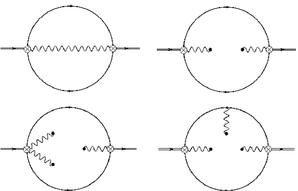
Figure 1: The Feynman diagrams that contribute to $\Pi_{0}^{\text{QCD}}(q^{2})$ at LO in $\alpha_{s}$ up to and including 6d condensates. Feynman diagrams were drawn with JaxoDraw [21].

On the right-hand side of (5), we use a resonances-plus-continuum model,

$$\frac{1}{\pi}\mathrm{Im}\Pi_{0}(t)=\rho^{\text{had}}(t)+\theta(t-s_{0})\frac{1}{\pi}\mathrm{Im}\Pi^{\text{QCD}}_{0}(t),$$ (10)

where $\rho^{\text{had}}(t)$ represents the resonance content of $\mathrm{Im}\Pi_{0}(t)$, $\theta(t)$ is the Heaviside step function, and $s_{0}$ is the continuum threshold parameter.

In (5), to eliminate the (generally unknown) subtraction constants and to accentuate the low-energy contribution of $\mathrm{Im}\Pi_{0}(t)$ to the integral, we consider (continuum-) subtracted LSRs, $\mathcal{R}_{k}(\tau,\,s_{0})$, of (usually nonnegative) integer weight $k$ at Borel scale $\tau$,

$$\mathcal{R}_{k}(\tau,\,s_{0})=\mathcal{R}_{k}(\tau)-\int_{s_{0}}^{\infty}\!t^{k}e^{-t\tau}\frac{1}{\pi}\mathrm{Im}\Pi_{0}^{\text{QCD}}(t)\,\mathrm{d}t,$$ (11)

in terms of unsubtracted LSRs, $\mathcal{R}_{k}(\tau)$, defined by

$$\mathcal{R}_{k}(\tau)=\frac{1}{\tau}\lim_{\stackrel{{\scriptstyle N,Q^{2}\rightarrow\infty}}{{\tau=N/Q^{2}}}}\frac{\big{(}-Q^{2}\big{)}^{N}}{\Gamma(N)}\bigg{(}\frac{d}{dQ^{2}}\bigg{)}^{N}\left\{(-Q^{2})^{k}\Pi_{0}(Q^{2})\right\},$$ (12)

where $Q^{2}=-q^{2}$ [1, 2, 3]. Equations (5) and (10)–(12) together imply

$$\mathcal{R}_{k}(\tau,\,s_{0})=\int_{t_{0}}^{\infty}\!t^{k}e^{-t\tau}\rho^{\text{had}}(t)\mathrm{d}t.$$ (13)

Details on how to compute $\mathcal{R}_{k}(\tau,\,s_{0})$ for a correlator such as (8) can be found in the literature (e.g., [1, 17, 18]). The result can be expressed as

$$\mathcal{R}_{k}(\tau,\,s_{0})=\int_{4m_{c}^{2}(1+\eta)}^{s_{0}}\!t^{k}e^{-t\tau}\frac{1}{\pi}\mathrm{Im}\Pi_{0}^{\text{QCD}}(t)\,\mathrm{d}t+\frac{1}{2\pi i}\int_{\Gamma_{\eta}}\!\left(q^{2}\right)^{k}e^{-q^{2}\tau}\Pi_{0}^{\text{QCD}}(q^{2})\,\mathrm{d}q^{2}$$ (14)

where $\Gamma_{\eta}$ is a circle in the complex $q^{2}$-plane of arbitrary radius $\eta$ centred at $q^{2}=4m_{c}^{2}$ which we parameterize by

$$q^{2}=4m_{c}^{2}\left(1+\eta e^{i\theta}\right)$$ (15)

for $\theta_{i}=2\pi^{-}$ to $\theta_{f}=0^{+}$. For $t\geq 4m_{c}^{2}$, as computed in [18], we have that

$$\mathrm{Im}\Pi_{0}^{\text{QCD}}(t)=\frac{\alpha_{s}m_{c}^{6}}{120\pi^{2}z^{2}}\Bigg{(}\sqrt{z(z-1)}(30-115z+166z^{2}+8z^{3}+16z^{4})\\ -15(-2+9z-16z^{2}+16z^{3})\log\big{(}\sqrt{z-1}+\sqrt{z}\big{)}\Bigg{)}\\ +\frac{m_{c}^{2}}{12}\sqrt{1-\frac{1}{z}}(2z+1)\langle\alpha G^{2}\rangle+\frac{1}{256\pi z(z-1)^{2}}\sqrt{1-\frac{1}{z}}(2z^{2}-2z+1)\langle g^{3}G^{3}\rangle$$ (16)

where

$$z=\frac{t}{4m_{c}^{2}}.$$ (17)

To implement renormalization-group improvement, we replace the strong coupling and the charm quark mass in (8) and (16) by one-loop, $\overline{\text{MS}}$ running quantities at four flavours [22]:

$$\alpha_{s}(\mu)=\frac{\alpha_{s}\left(m_{\tau}\right)}{1+\frac{25}{12\pi}\alpha_{s}\left(m_{\tau}\right)\log(\frac{\mu^{2}}{m_{\tau}^{2}})}$$ (18)

$$m_{c}(\mu)=m_{c}(\overline{m}_{c})\left(\frac{\alpha_{s}(\mu)}{\alpha_{s}(\overline{m}_{c})}\right)^{\frac{12}{25}}$$ (19)

where [23]

$$m_{\tau}=(1.77686\pm 0.00012)\ \text{GeV}$$ (20)

$$\alpha_{s}(m_{\tau})=0.330\pm 0.014$$ (21)

$$\overline{m}_{c}=(1.275\pm 0.025)\ \text{GeV}.$$ (22)

Also, we set $\mu=\overline{m}_{c}$.

3 Methods and results

We compute the LSRs, $\mathcal{R}_{k}(\tau,\,s_{0})$, (see (14)) of weight $k=0$ and $k=1$ using pySecDec-determined numerical results for $\Pi^{\text{QCD}}_{0}(q^{2})$ and $\mathrm{Im}\Pi_{0}^{\text{QCD}}(t)$ rather than using the analytic expressions (8) and (16) respectively.

But first, we must decide on a value for the arbitrary parameter $\eta$ in (14). The correlator (8) has a branch cut along the positive real semi-axis originating at the branch point $z=1$, i.e., $q^{2}=4m_{c}^{2}$. Near the branch point, the 6d gluon condensate OPE term is unbounded. Also, the imaginary part of the 4d gluon condensate term steeply approaches the branch point from above. Such behaviour is common and corresponds to large values of $|\frac{\mathrm{d}}{\mathrm{d}q^{2}}\Pi_{0}^{\text{QCD}}(q^{2})|$ near $q^{2}=4m_{c}^{2}$. To improve the reliability of numerical integration methods, it is advantageous to avoid these large-magnitude derivatives by choosing a large value for $\eta$. However, because of the exponential factor, $e^{-q^{2}\tau}$, in the integrand of the second integral on the right-hand side of (14), it is also advantageous to ensure that $\mathrm{Re}(q^{2})>0$ along $\Gamma_{\eta}$. Both advantages are realized by choosing $\eta$ slightly less than 1; in our case, $\eta=0.999$.

Regarding $\tau$, we consider $0.1\ \text{GeV}^{-2}\leq\tau\leq 0.5\ \text{GeV}^{-2}$, a range that easily covers the $\tau$-interval used in the LSRs analysis of [18]. Regarding $s_{0}$, we restrict our attention to $s_{0}>8m_{c}^{2}$, consistent with our choice of $\eta$. As for an upper bound on $s_{0}$, in some LSRs analyses, it is useful to compute $\mathcal{R}_{k}(\tau,\,s_{0})$ as $s_{0}\rightarrow\infty$. However, because of the exponential damping factor, $e^{-t\tau}$, in the integrand of the first integral on the right-hand side (14), the $s_{0}\rightarrow\infty$ limit can be practically calculated by simply evaluating $\mathcal{R}_{k}(\tau,\,s_{0})$ at some large value of $s_{0}$. For the case under consideration, a maximum value $s_{0}\approx 120\ \text{GeV}^{2}$ is large enough by a comfortable margin.

We compute each of the two integrals on the right-hand side of (14) using Simpson’s rule. For the first integral, we use sample points $\{t_{n}\}_{n=0}^{144}$ where

$$t_{n}=4m_{c}^{2}(1.02^{n}+\eta)$$ (23)

which unevenly spans the range $8m_{c}^{2}\lesssim t\lesssim 120\ \text{GeV}^{2}$. The adaptive step-sizing of (23) emphasizes the behaviour of the integrand near the lower limit of integration where the exponential damping is smallest, and is needed for Simpson’s rule to give accurate results for large $s_{0}$. Note that, for $s_{0}<120\ \text{GeV}^{2}$, not all of the sample points (23) are used. For example, at the value $s_{0}=25\ \text{GeV}^{2}$, only the first 53 grid points are used to numerically evaluate the integral in question. In figs. 2 and 3, we plot the analytic result for $\mathrm{Im}\Pi_{0}^{\text{QCD}}(t)$ from (16) along with corresponding numerical pySecDec-calculated results at the sample points (23). For the second integral on the right-hand side of (14), we use 123 sample points evenly spaced along the circle $\Gamma_{\eta}$. Because

$$\Pi_{0}^{\text{QCD}}\big{(}(q^{2})^{*}\big{)}=\Big{(}\Pi_{0}^{\text{QCD}}(q^{2})\Big{)}^{*},$$ (24)

we only need to use pySecDec to evaluate $\Pi_{0}^{\text{QCD}}(q^{2})$ for those sample points $q^{2}$ satisfying $\mathrm{Im}(q^{2})\geq 0$. We don’t directly compare the analytic result for $\Pi_{0}^{\text{QCD}}(q^{2})$ in (8) to pySecDec-calculated results because (as noted in sect. 2) an irrelevant polynomial has been omitted from (8). In fig. 4, we compare the $k=0$ LSRs (14) calculated using analytic results for $\Pi_{0}^{\text{QCD}}(q^{2})$ and $\mathrm{Im}\Pi_{0}^{\text{QCD}}(t)$ (i.e., (8) and (16) respectively) and using pySecDec-generated results at a selection of $s_{0}$-values. Figure 5 is analogous to fig. 4, but for $k=1$ rather than $k=0$ LSRs.

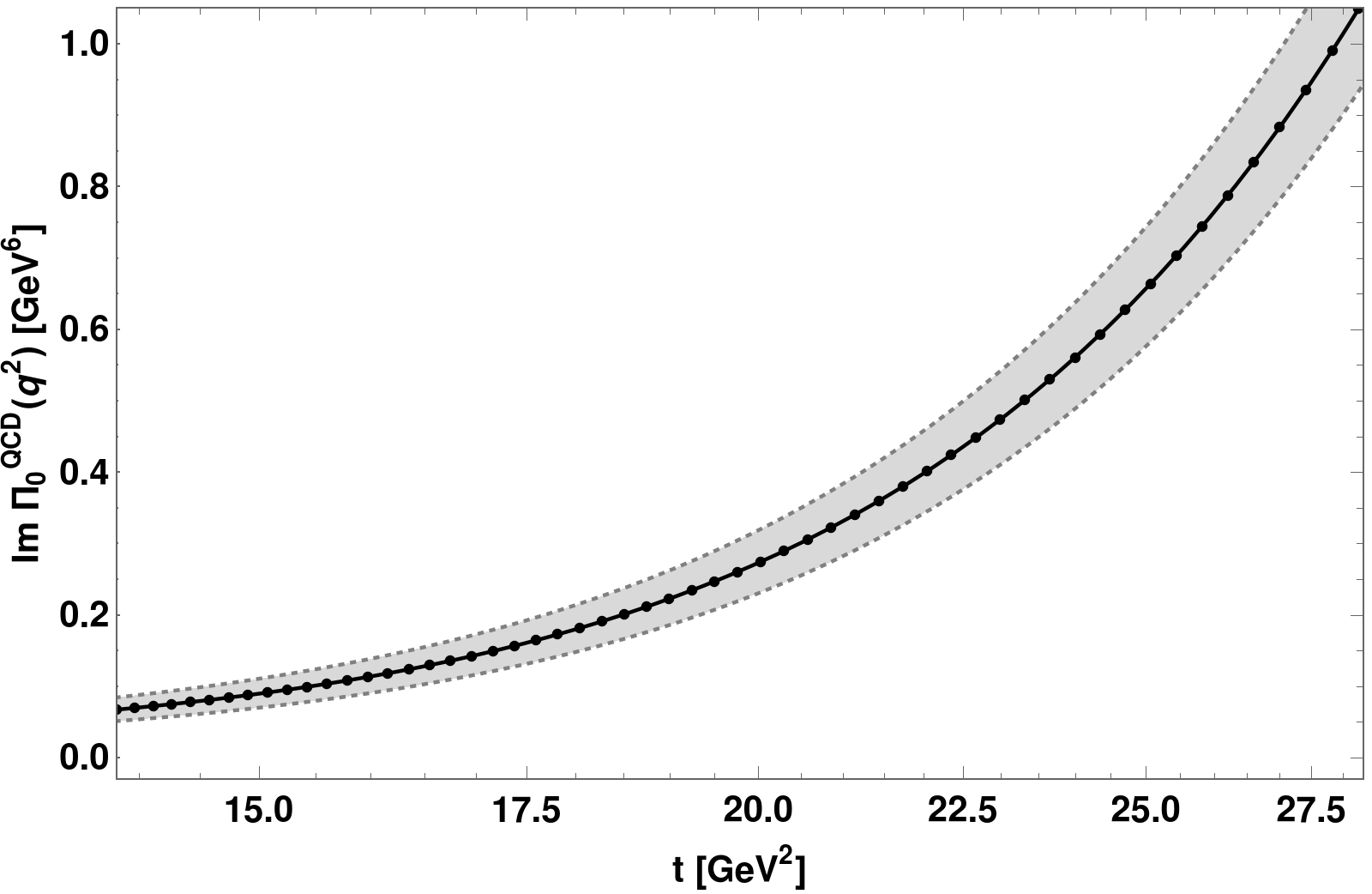
Figure 2: Comparison of $\mathrm{Im}\Pi_{0}^{\text{QCD}}(t)$ calculated analytically (see (16)) and numerically using pySecDec. (Note the logarithmic horizontal axis.) The solid line represents the analytic result with central values of $\langle\alpha G^{2}\rangle$, $\langle g^{3}G^{3}\rangle$, $\alpha_{s}(m_{\tau})$, and $\overline{m}_{c}$ (see (6), (7), (21), and (22) respectively). The two dotted lines represent upper and lower bounds on the analytic result that take into account uncertainties in $\langle\alpha G^{2}\rangle$, $\langle g^{3}G^{3}\rangle$, $\alpha_{s}(m_{\tau})$, and $\overline{m}_{c}$. The dots represent pySecDec-generated results at those values of the grid points (23) which satisfy $t\lesssim 28\ \text{GeV}^{2}$. The relative uncertainties of the pySecDec-generated results are of the order $10^{-7}$, and the corresponding error bars are much smaller than the dots used in the figure.

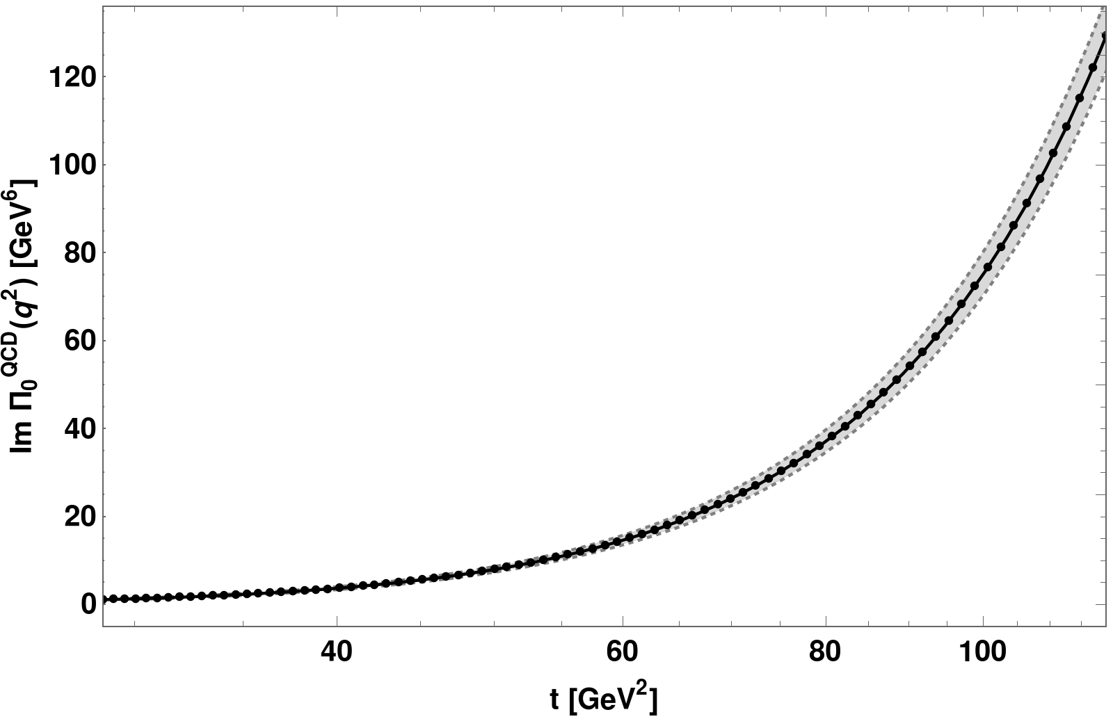
Figure 3: The same as fig. 2 but for a larger range of $t$-values.

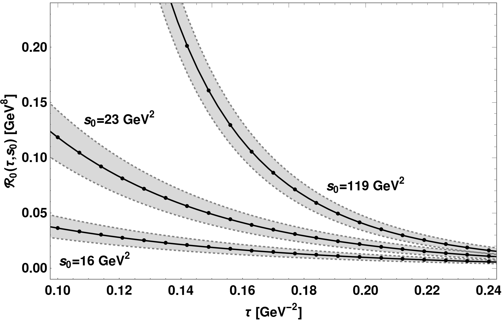
Figure 4: Comparison of the $k=0$ LSRs, $\mathcal{R}_{0}(\tau,\,s_{0})$, (see (14)) calculated using analytic results for $\Pi_{0}^{\text{QCD}}(q^{2})$ and $\mathrm{Im}\Pi_{0}^{\text{QCD}}(t)$ (see (8) and (16) respectively) and using pySecDec-generated numerical results at a representative set of continuum threshold parameter values, $s_{0}=16\ \text{GeV}^{2}$, $s_{0}=23\ \text{GeV}^{2}$, and $s_{0}=119\ \text{GeV}^{2}$. The solid lines represent LSRs computed using analytic results with central values of $\langle\alpha G^{2}\rangle$, $\langle g^{3}G^{3}\rangle$, $\alpha_{s}(m_{\tau})$, and $\overline{m}_{c}$ (see (6), (7), (21), and (22) respectively). Dotted lines represent upper and lower bounds on the solid lines that take into account uncertainties in $\langle\alpha G^{2}\rangle$, $\langle g^{3}G^{3}\rangle$, $\alpha_{s}(m_{\tau})$, and $\overline{m}_{c}$. The dots represent LSRs computed at a representative discrete collection of $\tau$-values using pySecDec-generated numerical results for $\Pi_{0}^{\text{QCD}}(q^{2})$ and $\mathrm{Im}\Pi_{0}^{\text{QCD}}(t)$. The relative uncertainties due to pySecDec are, at worst, on the order of $10^{-4}$, and the corresponding error bars are much smaller than the dots in the figure.

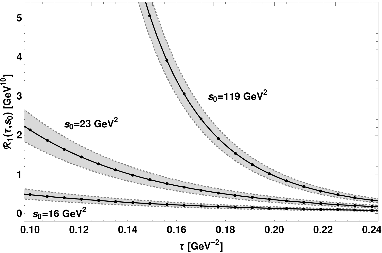
Figure 5: The same as fig. 4 but for $k=1$ LSRs, $\mathcal{R}_{1}(\tau,\,s_{0})$.

4 Discussion

From figs. 2 and 3, we see that there is exceptional agreement between $\mathrm{Im}\Pi_{0}^{\text{QCD}}(t)$ computed analytically (see (16)) and numerically using pySecDec over the entire range $8m_{c}^{2}\lesssim t\lesssim 120\ \text{GeV}^{2}$. The relative errors between true values (i.e., those computed analytically) and pySecDec-calculated values are of the order $10^{-9}$. Also, for the pySecDec-calculated results (i.e., the dots in the two figures), the relative uncertainties as reported by pySecDec are of the order $10^{-7}$, and the corresponding error bars are far too small to be seen in the two figures. And so, the pySecDec-generated errors are much smaller than the pySecDec-generated uncertainties which, in turn, are negligible compared to the uncertainties in $\mathrm{Im}\Pi_{0}^{\text{QCD}}(t)$ associated with experimental uncertainties in the QCD parameters, $\langle\alpha G^{2}\rangle$, $\langle g^{3}G^{3}\rangle$, $\alpha_{s}(m_{\tau})$, and $\overline{m}_{c}$ (see (6), (7), (21), and (22) respectively). In principle, the uncertainties attributable to pySecDec could be reduced at the cost of longer pySecDec runtimes. Note that the total pySecDec runtime needed to produce the data points in figs. 2 and 3 was a few hours on a mid-range laptop.

Similarly, from figs. 4 and 5, we see that there is excellent agreement between the LSRs, $\mathcal{R}_{0}(\tau,\,s_{0})$ and $\mathcal{R}_{1}(\tau,\,s_{0})$, computed using the analytic results (8) and (16) and pySecDec-calculated equivalents. The relative errors between true values and values determined numerically are of the order $10^{-5}$ or less. This conclusion holds for the entire range of $s_{0}$-values considered (i.e., $8m_{c}^{2}\lesssim s_{0}\lesssim 120\ \text{GeV}^{2}$) and the entire range of $\tau$-values considered (i.e., $0.1\ \text{GeV}^{-2}\leq\tau\leq 0.5\ \text{GeV}^{-2}$), not just at the particular $s_{0}$-values and $\tau$-values used in figs. 4 and 5. The relative uncertainties in the numerically-computed LSRs attributable to pySecDec are of the order $10^{-4}$ or less. Of course, there are also uncertainties in the numerically-computed LSRs associated with Simpson’s rule. We have made no attempt to quantify these uncertainties, but note that they decrease rapidly with increasing numbers of sample points. And so, computing here the LSRs $\mathcal{R}_{0}(\tau,\,s_{0})$ and $\mathcal{R}_{1}(\tau,\,s_{0})$ using a combination of pySecDec and Simpson’s rule produced errors that were an order of magnitude smaller than the uncertainties attributable to pySecDec which, in turn, were negligible compared to the uncertainties attributable to the parameters of QCD, $\langle\alpha G^{2}\rangle$, $\langle g^{3}G^{3}\rangle$, $\alpha_{s}(m_{\tau})$, and $\overline{m}_{c}$.

In addition to LSRs, there are other variants of QCD sum-rules used in the literature. Two such variants are FESRs, $\mathcal{F}_{k}(s_{0})$, [24, 4]

$$\mathcal{F}_{k}(s_{0})=\int_{4m_{c}^{2}(1+\eta)}^{s_{0}}\!t^{k}\frac{1}{\pi}\mathrm{Im}\Pi_{0}^{\text{QCD}}(t)\,\mathrm{d}t+\frac{1}{2\pi i}\int_{\Gamma_{\eta}}\!\left(q^{2}\right)^{k}\Pi_{0}^{\text{QCD}}(q^{2})\,\mathrm{d}q^{2}$$ (25)

and GSRs, $\mathcal{G}_{k}(\hat{s},\,\tau,\,s_{0})$, [25, 4, 26]

$$\mathcal{G}_{k}(\hat{s},\,\tau,\,s_{0})=\int_{4m_{c}^{2}(1+\eta)}^{s_{0}}\!t^{k}\frac{e^{-\frac{(\hat{s}-t)^{2}}{4\tau}}}{\sqrt{4\pi\tau}}\frac{1}{\pi}\mathrm{Im}\Pi_{0}^{\text{QCD}}(t)\,\mathrm{d}t+\frac{1}{2\pi i}\int_{\Gamma_{\eta}}\!\left(q^{2}\right)^{k}\frac{e^{-\frac{-(\hat{s}-q^{2})^{2}}{4\tau}}}{\sqrt{4\pi\tau}}\Pi_{0}^{\text{QCD}}(q^{2})\,\mathrm{d}q^{2}.$$ (26)

The difference between LSRs (14) and either FESRs (25) or GSRs (26) is the kernel of the integrands, i.e., a decaying exponential in LSRs, a trivial kernel in FESRs, and a Gaussian in GSRs. On the left-hand side of (26), in addition to the continuum threshold $s_{0}$, there are two other independent variables: $\hat{s}$, the position of the peak of the Gaussian kernel (in $\text{GeV}^{2}$) and $\tau$, the variance of the Gaussian kernel (in $\text{GeV}^{4}$). (Despite the same letter $\tau$ being used in the definitions of LSRs and GSRs, the two parameters are not the same.) The pySecDec-determined correlator results for $\Pi_{0}^{\text{QCD}}(q^{2})$ and $\mathrm{Im}\Pi_{0}^{\text{QCD}}(t)$ can be used to numerically evaluate (25) and (26) using the same procedure as that described in Section 3 for LSRs. The integration contour of Section 3 was chosen with LSRs in mind; nevertheless, we find excellent agreement between FESRs and GSRs computed using analytic correlator results and pySecDec-computed correlator results. For FESRs, we find relative errors less than $10^{-5}$ for $k\in\{0,\,1\}$ over the entire range of $s_{0}$ values considered, i.e. $8m_{c}^{2}\lesssim s_{0}\lesssim 120~{}\text{GeV}^{2}$. For GSRs, we find relative errors less than $10^{-4}$ for $k\in\{0,\,1\}$ over the entire range of $s_{0}$ values considered and where $10\ \text{GeV}^{4}\leq\tau\leq 20\ \text{GeV}^{4}$ (a range consistent with the discussion in [26]) and $-5\ \text{GeV}^{2}\leq\hat{s}\leq 40\ \text{GeV}^{2}$ (a range that covers essentially all of the area underneath $\mathcal{G}_{k}(\hat{s},\,\tau,\,s_{0})$ for the range of $\tau$ values considered and for realistic values of $s_{0}$.)

For the pseudoscalar charmonium hybrid correlator considered in this article ($\Pi_{0}$ on the right-hand side of (4)), the dimensionally-regularized Feynman diagrams of fig. 1 could be evaluated analytically yielding (8). Corresponding LSRs, FESRs, and GSRs could then be computed in a straightforward fashion. In this article, as an alternative, we explicitly showed that QCD sum-rules computed numerically using a combination of pySecDec and Simpson’s rule were in excellent agreement with those constructed from an analytic expression for $\Pi_{0}$. As Feynman diagrams get increasingly complicated due to larger numbers of loops, external lines, and/or masses, evaluating them analytically can become prohibitively difficult. In such cases, evaluating the diagrams and computing corresponding QCD sum-rules with the help of pySecDec is a viable option.

References

- [1] M. A. Shifman, A. I. Vainshtein, and V. I. Zakharov, Nucl. Phys. B147, 448 (1979).
- [2] M. A. Shifman, A. I. Vainshtein, and V. I. Zakharov, Nucl. Phys. B147, 385 (1979).
- [3] L. J. Reinders, H. Rubinstein, and S. Yazaki, Phys. Rept. 127, 1 (1985).
- [4] S. Narison, QCD as a Theory of Hadrons, Vol. 17 (Cambridge University Press, 2007).
- [5] K. G. Wilson, Phys. Rev. 179, 1499 (1969).
- [6] P. Pascual and R. Tarrach, QCD: Renormalization for the Practitioner (Springer, 1984).
- [7] E. E. Boos and A. I. Davydychev, Theor. Math. Phys. 89, 1052 (1991).
- [8] A. I. Davydychev, J. Math. Phys. 33, 358 (1992).
- [9] D. J. Broadhurst, J. Fleischer, and O. V. Tarasov, Z. Phys. C60, 287 (1993), hep-ph/9304303v1.
- [10] J. A. M. Vermaseren, (2000), math-ph/0010025.
- [11] J. Kuipers, T. Ueda, and J. A. M. Vermaseren, Comput. Phys. Commun. 189, 1 (2015), 1310.7007.
- [12] B. Ruijl, T. Ueda, and J. Vermaseren, (2017), 1707.06453.
- [13] M. Galassi, J. Davies, J. Theiler, B. Gough, G. Jungman, P. Alken, M. Booth, and F. Rossi, GNU Scientific Library Reference Manual, 3 ed. (Network Theory Ltd., 2009).
- [14] T. Hahn, Comput. Phys. Commun. 168, 78 (2005), hep-ph/0404043.
- [15] T. Hahn, J. Phys. Conf. Ser. 608, 012066 (2015), 1408.6373.
- [16] S. Borowka, G. Heinrich, S. Jahn, S. P. Jones, M. Kerner, J. Schlenk, and T. Zirke, Comput. Phys. Commun. 222, 313 (2018), 1703.09692.
- [17] J. Govaerts, L. J. Reinders, and J. Weyers, Nucl. Phys. B262, 575 (1985).
- [18] R. Berg, D. Harnett, R. T. Kleiv, and T. G. Steele, Phys. Rev. D86, 034002 (2012), 1204.0049.
- [19] G. Launer, S. Narison, and R. Tarrach, Z. Phys. C26, 433 (1984).
- [20] S. Narison, Phys. Lett. B693, 559 (2010).
- [21] D. Binosi and L. Theussl, Compute. Phys. Commun. 161, 76 (2004).
- [22] S. Narison and E. de Rafael, Phys. Lett. B103, 57 (1981).
- [23] Particle Data Group, C. Patrignani et al., Chin. Phys. C40, 100001 (2016).
- [24] R. Shankar, Phys. Rev. D15, 755 (1977).
- [25] R. A. Bertlmann, G. Launer, and E. de Rafael, Nucl. Phys. B250, 61 (1985).
- [26] J. Ho, R. Berg, T. Steele, W. Chen, and D. Harnett, accepted in Phys. Rev. D (2018), 1709.06538.