$q$-Neurons: Neuron Activations based on Stochastic Jackson’s Derivative Operators

Abstract

We propose a new generic type of stochastic neurons, called $q$-neurons, that considers activation functions based on Jackson’s $q$-derivatives, with stochastic parameters $q$. Our generalization of neural network architectures with $q$-neurons is shown to be both scalable and very easy to implement. We demonstrate experimentally consistently improved performances over state-of-the-art standard activation functions, both on training and testing loss functions.

1 Introduction

The vanilla method to train a Deep Neural Network (DNN) is to use the Stochastic Gradient Descent (SGD) method (a first-order local optimization technique). The gradient of the DNN loss function, represented as a directed computational graph, is calculated using the efficient backpropagation algorithm relying on the chain rule of derivatives (a particular case of automatic differentiation).

The ordinary derivative calculus can be encompassed into a more general $q$-calculus [1, 2] by defining the Jackson’s $q$-derivative (and gradient) as follows:

$$D_{q}f(x):=\frac{f(x)-f(qx)}{(1-q)x},\quad q\neq 1,x\neq 0.$$ (1)

The $q$-calculus generalizes the ordinary Leibniz gradient (obtained as a limit case when $q\rightarrow 1$ or when $x\rightarrow 0$) but does not enjoy a generic chain rule property. It can further be extended to the $(p,q)$-derivative [8, 3] defined as follows:

$$D_{p,q}f(x):=\frac{f(px)-f(qx)}{(p-q)x}=D_{q,p}f(x),\quad p\neq{q},x\neq 0.$$ (2)

which encompasses the $q$-gradient as $D_{1,q}f(x)=D_{q,1}f(x)=D_{q}f(x)$.

The two main advantages of $q$-calculus are

1. To bypass the calculations of limits, and

2. To consider $q$ as a stochastic parameter.

We refer to the textbook [2] for an in-depth explanation of $q$-calculus. Appendix A recalls the basic rules and properties of the generic $(p,q)$-calculus [3] that further generalizes the $q$-calculus.

To the best of our knowledge, the $q$-derivative operators have seldom been considered in the machine learning community [11]. We refer to [4] for some encouraging preliminary experimental optimization results on global optimization tasks.

In this paper, we introduce a meta-family of neuron activation functions based on standard activation functions (e.g., sigmoid, softplus, ReLU, ELU). We refer to them as $q$-activations. The $q$-activation is a stochastic activation function built on top of any given activation function $f$. $q$-Activation is very easy to implement based on state-of-the-art Auto-Differentiation (AD) frameworks while consistently producing better performance. Based on our experiments, one should almost always use $q$-activation instead of its deterministic counterpart. In the remainder, we define $q$-neurons as stochastic neurons equipped with $q$-activations.

Our main contributions are summarized as follows:

• The generic $q$-activation and an analysis of its basic properties.

• An empirical study that demonstrates that the $q$-activation can reduce both training and testing errors.

• A novel connection and sound application of (stochastic) $q$-calculus in machine learning.

2 Neurons with $q$-activation functions

Given any activation function $f:\,\mathbb{R}\to\mathbb{R}$, we construct its corresponding “quantum” version, also called $q$-activation function, as

$$g_{q}(x):=\frac{f(x)-f(qx)}{1-q}=\left(D_{q}f(x)\right)x,$$ (3)

where $q$ is a real-valued random variable. To see the relationship between $g_{q}(x)$ and $f(x)$, let us observe that we have the following asymptotic properties:

Proposition 1.

Assume $f(x)$ is smooth and the expectation of $q$ is $E(q)=1$. Then $\forall{x}$, we have

$$\lim_{\mathrm{Var}(q)\to 0}g_{q}(x) =f^{\prime}(x)x.$$

$$\lim_{\mathrm{Var}(q)\to 0}g^{\prime}_{q}(x) =f^{\prime}(x)+f^{\prime\prime}(x)x,$$

where $E(\cdot)$ denotes the expectation, and $\mathrm{Var}(\cdot)$ denotes the variance.

Proof.

$$\lim_{\mathrm{Var}(q)\to 0}g_{q}(x)=\lim_{\mathrm{Var}(q)\to 0}\frac{f(x)-f(qx)}{x-qx}x=\lim_{qx\to{x}}\frac{f(x)-f(qx)}{x-qx}x=f^{\prime}(x)x.$$

$$\lim_{\mathrm{Var}(q)\to 0}g^{\prime}_{q}(x)=\lim_{\mathrm{Var}(q)\to 0}\frac{f^{\prime}(x)-qf^{\prime}(qx)}{1-q}=\lim_{\mathrm{Var}(q)\to 0}\frac{f^{\prime}(x)-qf^{\prime}(x)+qf^{\prime}(x)-qf^{\prime}(qx)}{1-q}$$

$$=f^{\prime}(x)+\lim_{\mathrm{Var}(q)\to 0}\frac{qf^{\prime}(x)-qf^{\prime}(qx)}{1-q}=f^{\prime}(x)+\lim_{q\to 1}\frac{f^{\prime}(x)-f^{\prime}(qx)}{x-qx}qx=f^{\prime}(x)+f^{\prime\prime}(x)x.$$

∎

Notice that as $\mathrm{Var}(q)\to 0$, the limit of $g_{q}(x)$ is not $f(x)$ but $f^{\prime}(x)x$. Thus informally speaking, the gradient of $g_{q}(x)$ carries second-order information of $f(x)$.

We further have the following property:

Proposition 2.

We have for $p,q\not=1$:

$$D_{p}(g_{q}(x))=\frac{1}{1-p}D_{q}f(x)-\frac{p}{1-p}D_{p,pq}f(x).$$ (4)

Proof.

$$D_{p}(g_{q}(x)) =\frac{g_{q}(x)-g_{q}(px)}{(1-p)x}=\frac{\left(D_{q}f(x)\right)x-\left(D_{q}f(px)\right)px}{(1-p)x}$$

$$=\frac{1}{1-p}D_{q}f(x)-\frac{p}{1-p}D_{q}f(px).$$ (5)

Since $D_{q}f(px)=\frac{f(px)-f(pqx)}{px-pqx}=\frac{f(px)-f(pqx)}{(p-pq)x}=D_{p,pq}f(x)$, eq. 4 is straightforward. ∎

By proposition 2, the $p$-derivative of the $q$-activation $g_{q}(x)$ agrees with the original activation function $f$.

See table 1 for a list of activation functions with their corresponding functions $f^{\prime}(x)x$, where

$$\operatorname{\mathrm{sigm}}(x)=1/(1+\exp(-x)),$$

is the sigmoid function,

$$\operatorname{\mathrm{softplus}}(x)=\log(1+\exp(x)),$$

is the softplus function,

$$\operatorname{\mathrm{relu}}(x)=\left\{\begin{array}[]{ll}x&\text{ if }x\geq 0\\ 0&\text{otherwise}\end{array}\right.$$

is the Rectified Linear Unit (ReLU) [5], and

$$\operatorname{\mathrm{elu}}(x)=\left\{\begin{array}[]{ll}x&\text{ if }x\geq 0\\ \alpha(\exp(x)-1)&\text{otherwise}\end{array}\right.$$

denotes the Exponential Linear Unit (ELU) [6].

Table 1: Common activation functions $f(x)$ with their corresponding limit cases $\lim_{\mathrm{Var}(q)\to 0}g_{q}(x)=f^{\prime}(x)x$.

$f(x)$	$\operatorname{\mathrm{sigm}}(x)$	$\tanh(x)$	$\operatorname{\mathrm{relu}}(x)$	$\operatorname{\mathrm{softplus}}(x)$	$\operatorname{\mathrm{elu}}(x)$
$f^{\prime}(x)x$	$\operatorname{\mathrm{sigm}}(x)(1-\operatorname{\mathrm{sigm}}(x))x$	$\mathrm{sech}^{2}(x)x$	$\mathrm{relu}(x)$	$\operatorname{\mathrm{sigm}}(x)x$	$\left\{\begin{array}[]{ll}x&x\geq 0\\ \alpha\exp(x)x&x<0\end{array}\right.$

A common choice for the random variable $q$ that is used in our experiments is

$$q=1+\left(2[\epsilon\geq 0]-1\right)\left(\lambda|\epsilon|+\phi\right),$$ (6)

where $\epsilon\sim N(0,1)$ follows the standard Gaussian distribution, $[\cdot]$ denotes the Iverson bracket (meaning $1$ if the proposition is satisfied, and $0$ otherwise), $\lambda>0$ is a scale parameter of $q$, and $\phi=10^{-3}$ is the smallest absolute value of $q$ so as to avoid division by zero. See fig. 1 for the density function plots of $q$ defined on $(-\infty,-\phi]\cup[\phi,\infty]$

Figure 1: The probability density function of stochastic variable $q$ (zero-avoiding) used when calculating $q$-derivatives.

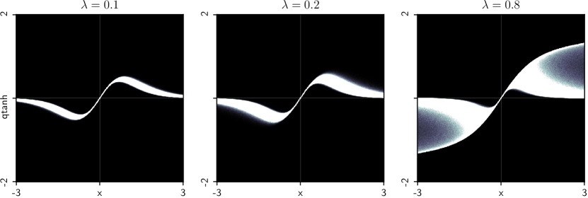
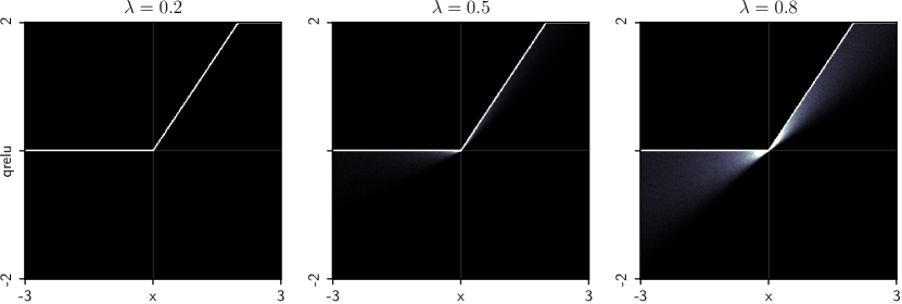
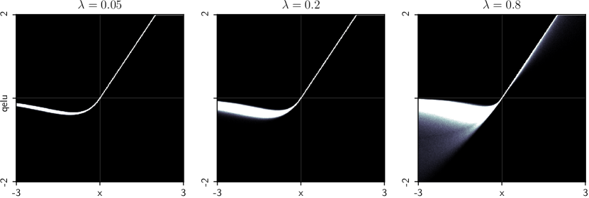
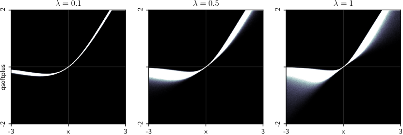
Figure 2: The density function of $q$-neurons with $q$ sampled according to eq. 6 for different values of $\lambda$. The activation is roughly a deterministic function $f^{\prime}(x)x$ for small $\lambda$ as shown in table 1. The activation is random for large $\lambda$. Darker color indicates higher probability density.

To implement $q$-neurons, one only need to tune the hyper-parameter $\lambda$. It can either be fixed to a small value, e.g. 0.02 or 0.05 during learning, or be annealed from an initial value $\lambda_{0}$. Such an annealing scheme can be set to

$$\lambda=\frac{\lambda_{0}}{1+\gamma(T-1)},$$ (7)

where $T=1,2,\cdots$ is the index of the current epoch, and $\gamma$ is a decaying rate parameter. This parameter $\gamma$ can be empirically fixed based on the total number of epochs: For example, in our experiments we train $100$ epochs and apply $\gamma=0.5$, so that in the final epochs $\lambda$ is a same value (around 0.02$\lambda_{0}$). We will investigate both of those two cases in our experiments.

Let us stress out that deep learning architectures based on stochastic $q$-neurons are scalable and easy to implement. There is no additional free parameter imposed. The computational overhead of $g_{q}(x)$ as compared to $f(x)$ involves sampling one Gaussian random variable, and then calling $f(x)$ two times and computing $g_{q}(x)$ according to eq. 3. In our Python implementation, the core implementation of $q$-neuron is only in three lines of codes (see A.3).

Alternative approaches to inject stochasticity into neural network training include dropout [13], gradient noise [12], etc. Both $q$-neuron and dropout modify the forward pass of the neural network. In the experimental section we will investigate the effect of $q$-neurons with or without dropout.

3 Experiments

We carried experiments on classifying MNIST digits and CIFAR10 images using Convolutional Neural Networks (CNNs) and Multi-Layer Perceptrons (MLPs). Our purpose is not to beat state-of-the-art records but to investigate the effect of applying $q$-neuron and its hyper-parameter sensitivity. We summarize the neural network architectures as follows:

• The MNIST-CNN architecture is given as follows: 2D convolution with $3\times 3$ kernel and $32$ features; ($q$-)activation; batch normalization; 2D convolution with $3\times 3$ kernel and $32$ features; ($q$-)activation; $2\times 2$ max-pooling; batch normalization; 2D convolution with $3\times 3$ kernel and $64$ features; ($q$-)activation; batch normalization; 2D convolution with $3\times 3$ kernel and $64$ features; ($q$-)activation; $2\times 2$ max-pooling; flatten into 1D vector; batch normalization; dense layer of output size $512$; ($q$-)activation; batch normalization; (optional) dropout layer with drop probability 0.2; dense layer of output size $10$; soft-max activation.

• The MNIST-MLP architecture is: dense layer of output size $256$; ($q$-)activation; batch normalization; (optional) dropout layer with drop probability 0.2; dense layer of output size $256$; ($q$-)activation; batch normalization; (optional) dropout layer with drop probability $0.2$; dense layer of output size $10$; soft-max activation.

• The CIFAR-CNN architecture is: 2D convolution with $3\times 3$ kernel and $32$ features; ($q$-)activation; 2D convolution with $3\times 3$ kernel and $32$ features; ($q$-)activation; $2\times 2$ max-pooling; (optional) dropout layer with drop probability 0.2; 2D convolution with $3\times 3$ kernel and $64$ features; ($q$-)activation; 2D convolution with $3\times 3$ kernel and $64$ features; ($q$-)activation; $2\times 2$ max-pooling; (optional) dropout layer with drop probability 0.2; flatten into 1D vector; dense layer of output size $512$; ($q$-)activation; (optional) dropout layer with drop probability 0.1; dense layer of output size $10$; soft-max activation.

We use the cross-entropy as the loss function. The model is trained for $100$ epochs based on a stochastic gradient descent optimizer with a mini-batch size of $64$ (MNIST) or $32$ (CIFAR) and a learning rate of 0.05 (MNIST) or 0.01 (CIFAR) without momentum. The learning rate is multiplied by $(1-10^{-6})$ after each mini-batch update. We compare $\tanh$, $\operatorname{\mathrm{relu}}$, $\operatorname{\mathrm{elu}}$, $\operatorname{\mathrm{softplus}}$ activations with their $q$-counterparts. We either fix $\lambda_{0}=0.02$ or $0.1$, or anneal from $\lambda_{0}\in\{1,5,9\}$ with $\gamma=0.5$. The learning curves are shown in figs. 3, 4 and 5, where the training curves show the sample-average cross-entropy values evaluated on the training set after each epoch, and the testing curves are classification accuracy. In all figures, each training or testing curve is an average over $10$ independent runs.

For $q$-activation, $c$ means the $\lambda$ parameter is fixed (’c’onstant); $a$ means the $\lambda$ is ’a’nnealed based on eq. 7. For example, “$c$0.02” means $\lambda=0.02$ throughout the training process, while “$a$1” means that $\lambda$ is annealed from $\lambda_{0}=1$.

We see that in almost all cases, $q$-activation can consistently improve learning, in the sense that both training and testing errors are reduced. This implies that $q$-neurons can get to a better local optimum as compared to the corresponding deterministic neurons. The exception worth noting is $q$-$\operatorname{\mathrm{relu}}$, which cannot improve over $\operatorname{\mathrm{relu}}$ activation. This is because $g_{q}(x)$ is very similar to the original $f(x)$ for (piece-wisely) linear functions. By proposition 1, $f^{\prime\prime}(x)=0$ implies that the gradient of $g_{q}(x)$ and $f(x)$ are similar for small $\mathrm{Var}(q)$. One is advised to use $q$-neurons only with curved activation functions such as $\operatorname{\mathrm{elu}}$, $\tanh$, etc.

We also observe that the benefits of $q$-neurons are not sensitive to hyper-parameter selection. In almost all cases, $q$-neuron with $\lambda$ simply fixed to 0.02/0.1 can bring better generalization performance, while an annealing scheme can further improve the score. Setting $\lambda$ too large may lead to under-fit. One can benefit from $q$-neurons either with or without dropout.

On the MNIST dataset, the best performance with error rate 0.35% (99.65% accuracy) is achieved by the CNN architecture with $q$-$\operatorname{\mathrm{elu}}$ and $q$-$\tanh$. On the CIFAR10 dataset, the best performance of the CNN with accuracy 82.9% is achieved by $q$-$\operatorname{\mathrm{elu}}$.

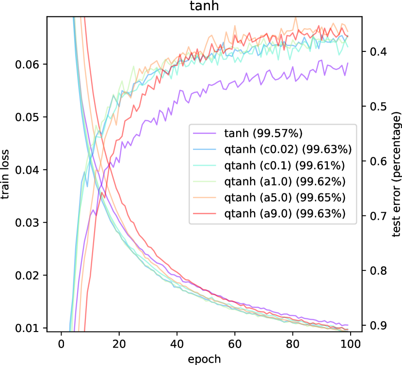
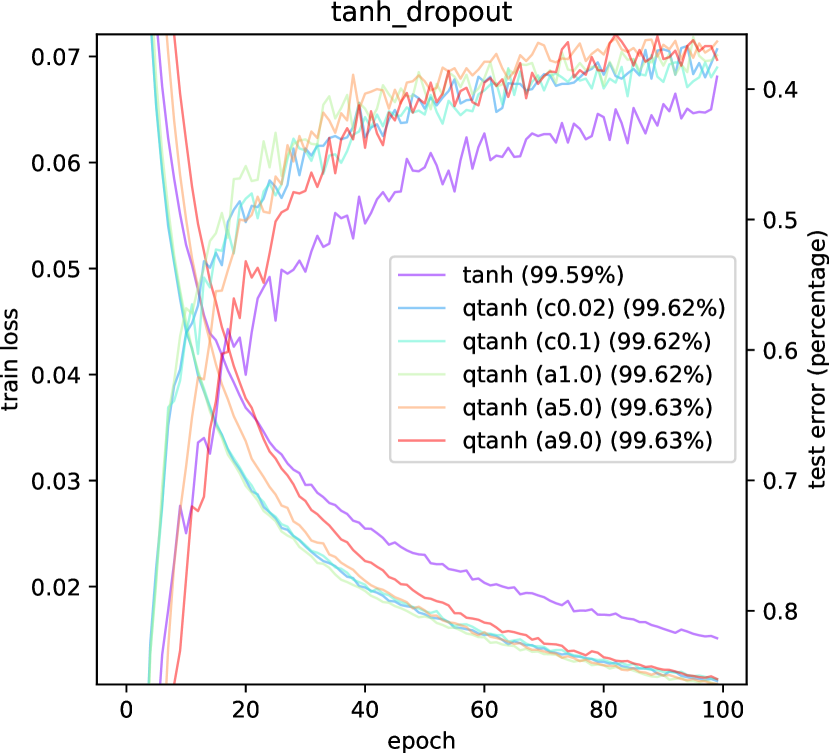
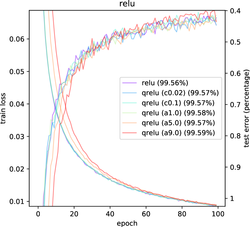
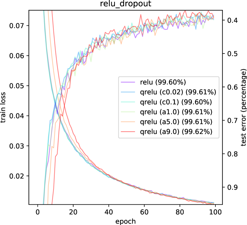
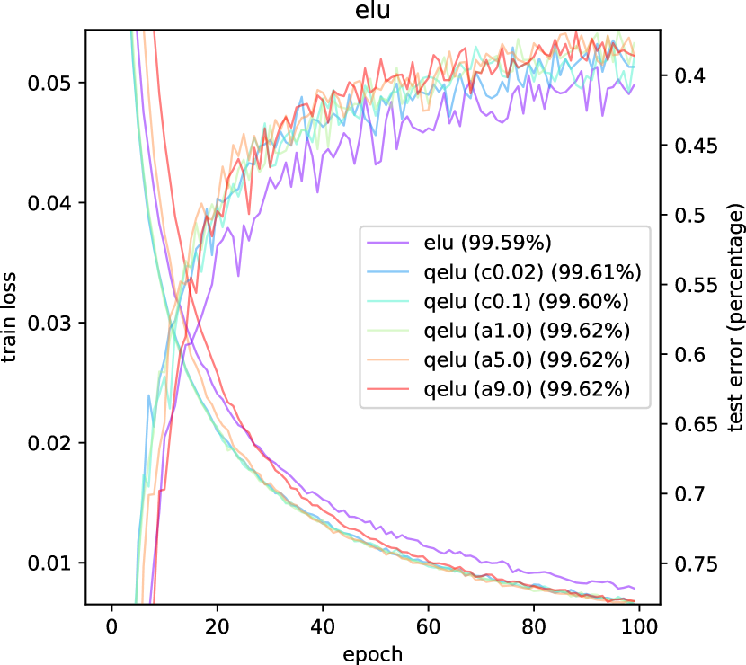
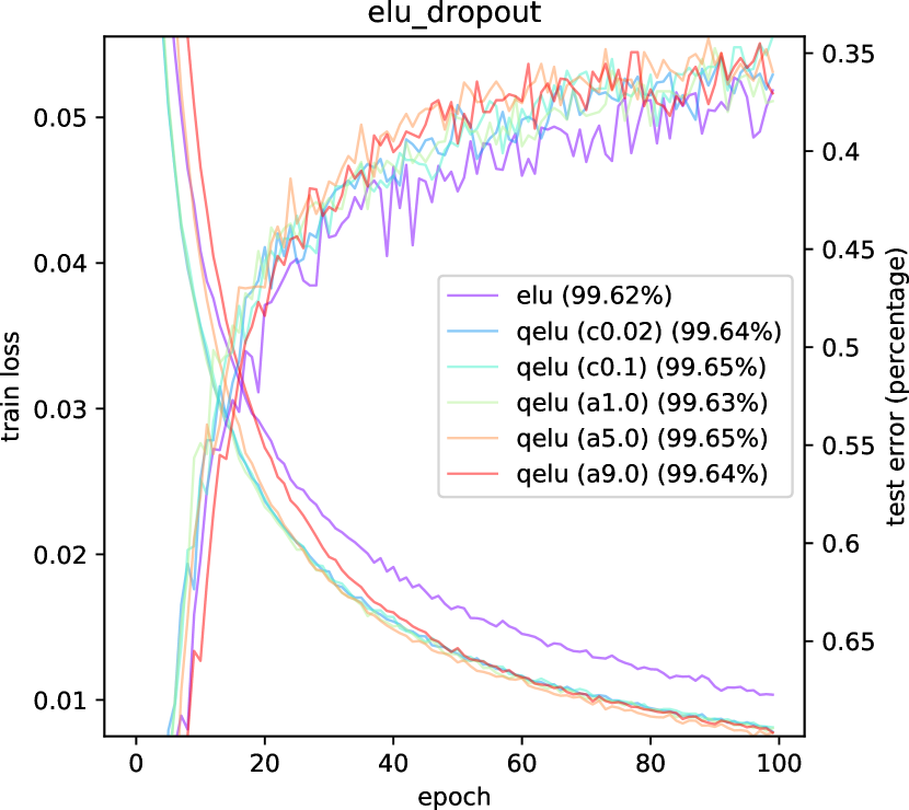
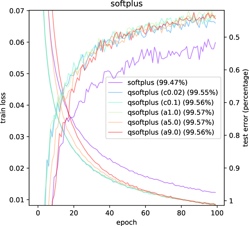
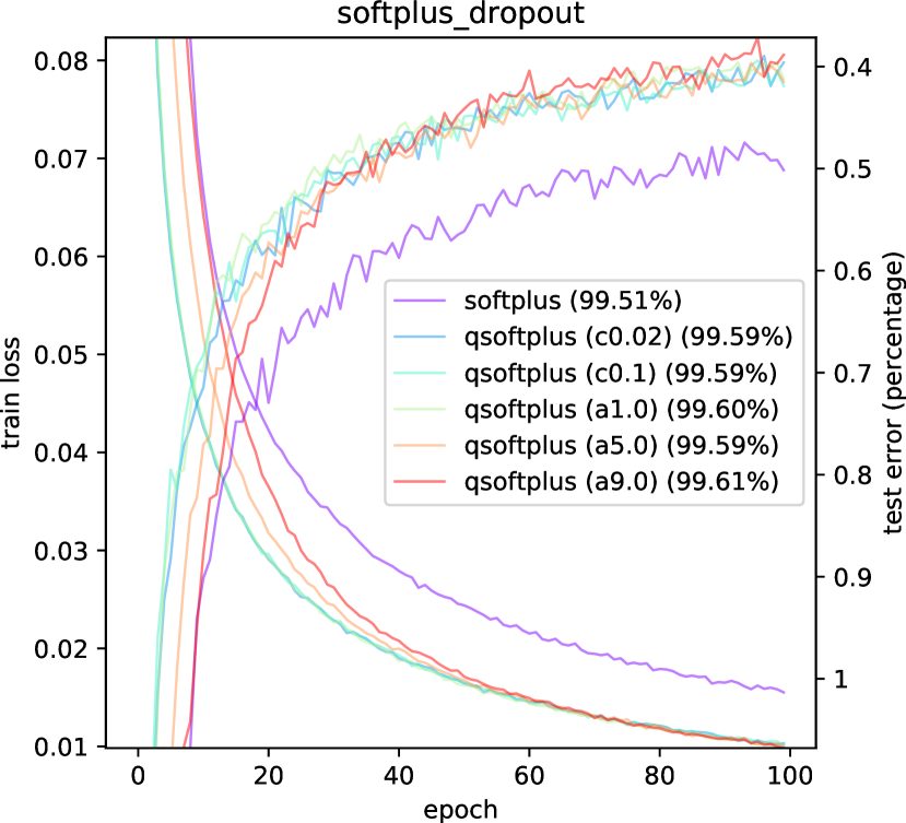
Figure 3: Training loss (descending curves) and testing accuracy (ascending curves) of a CNN on the MNIST dataset, using different activation functions (from top to bottom), with (left) or without (right) dropout.

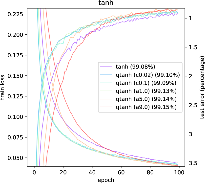
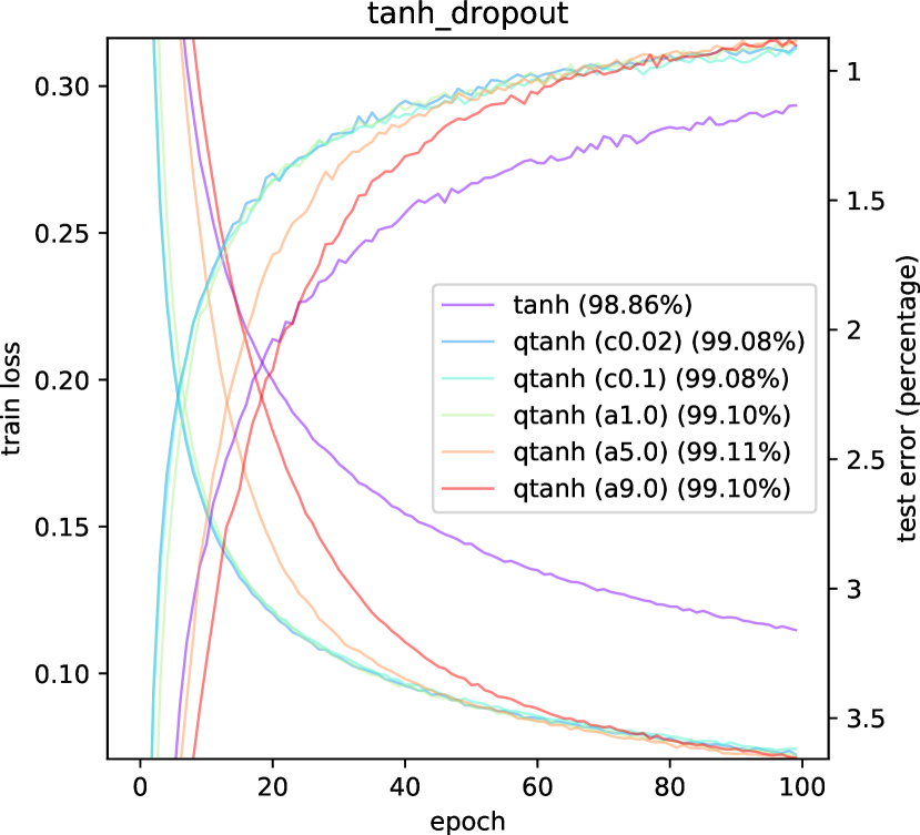
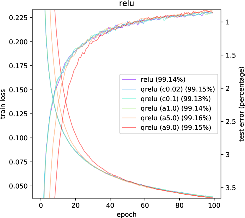
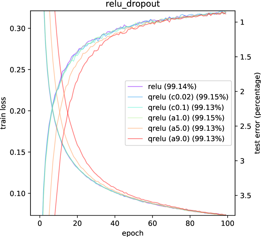
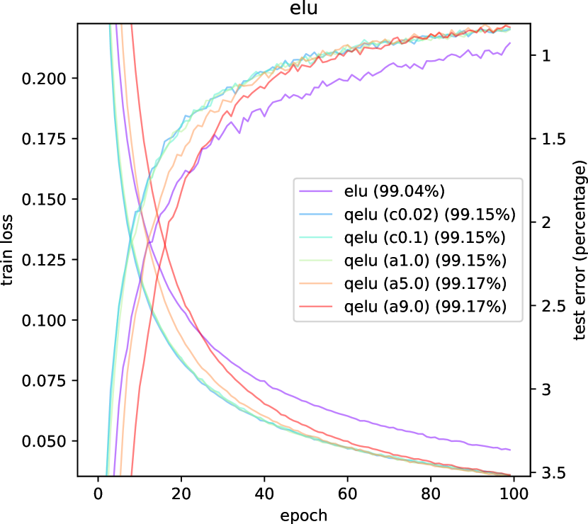
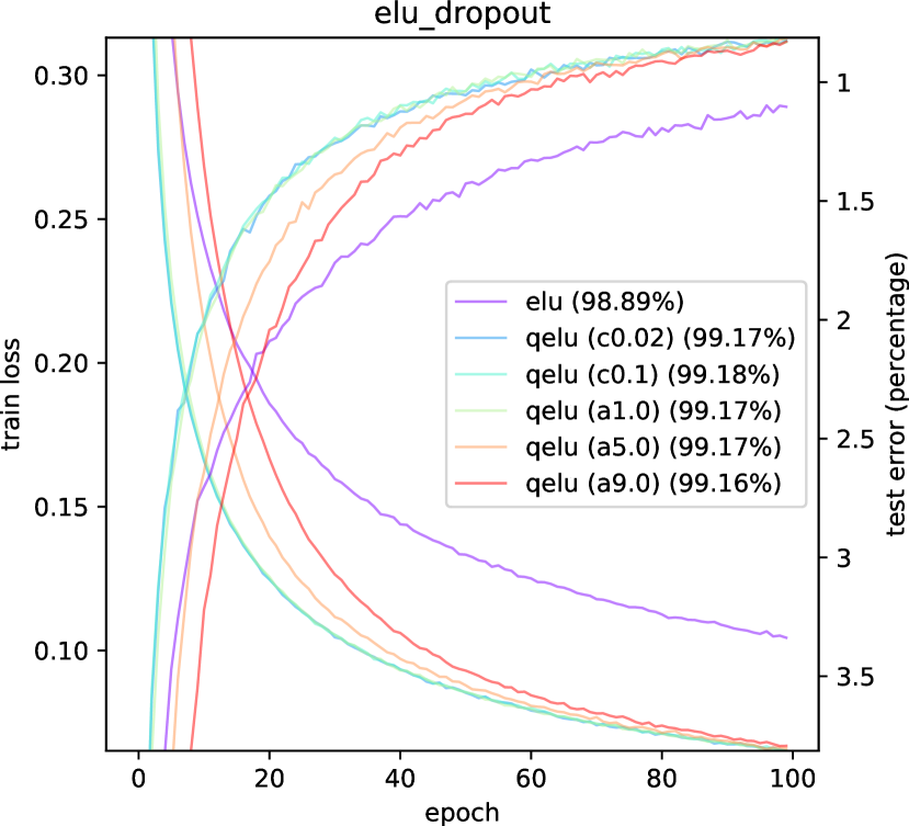
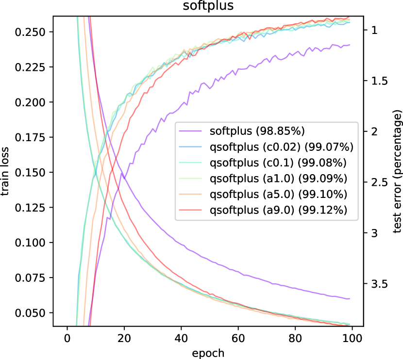
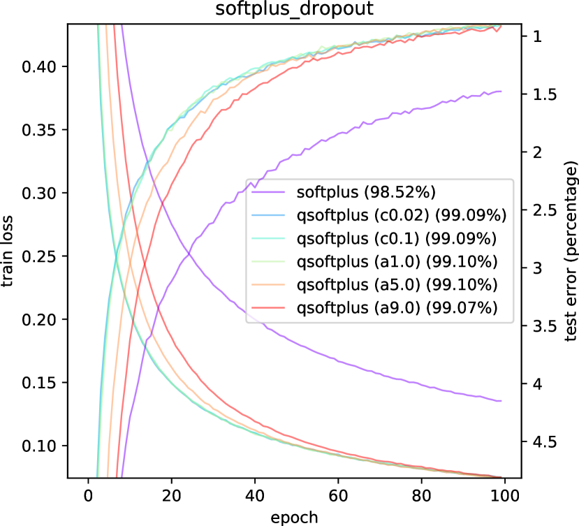
Figure 4: Training loss (descending curves) and testing accuracy (ascending curves) of a MLP on MNIST.

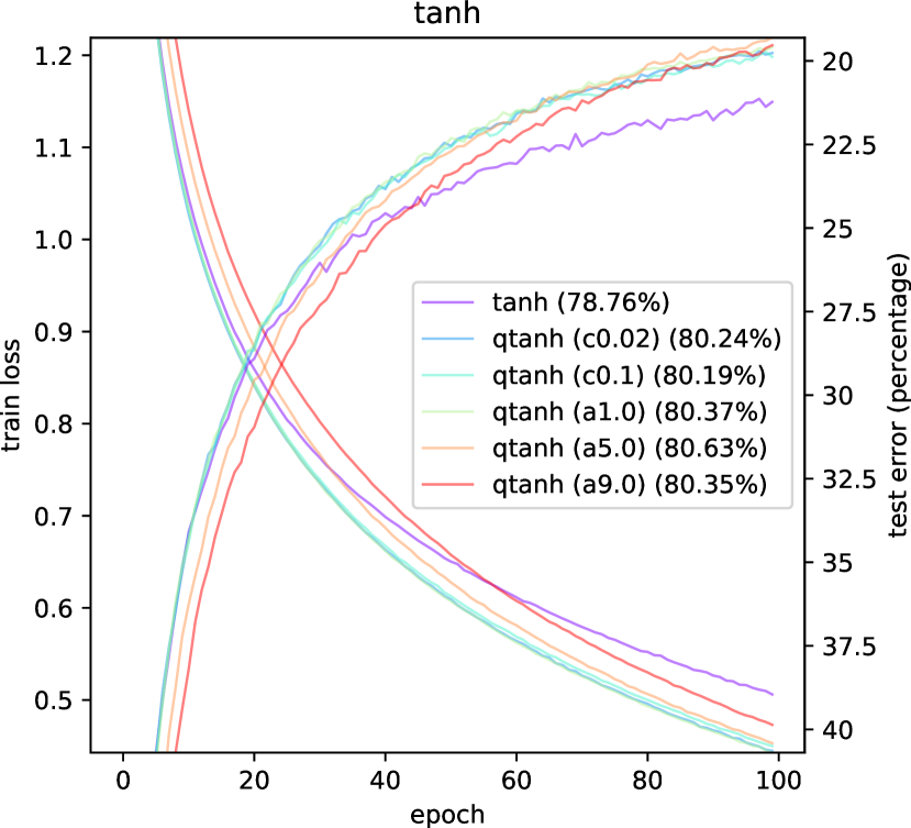
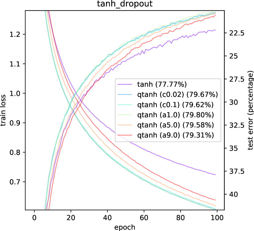
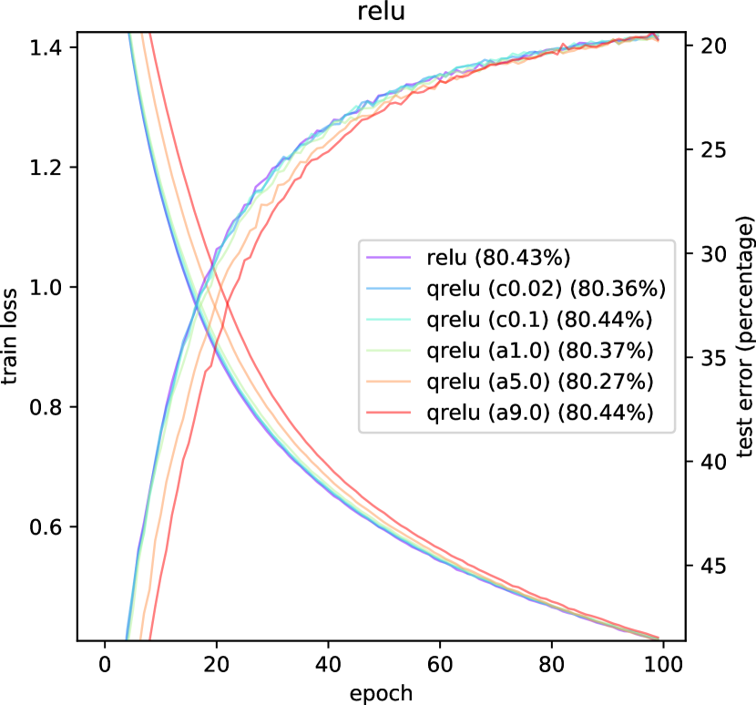
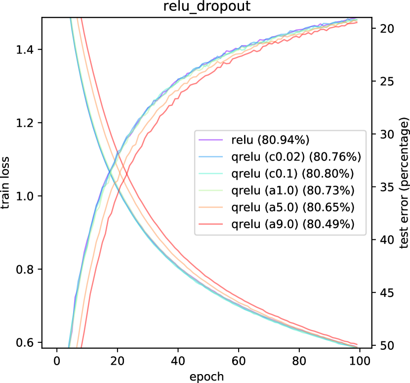
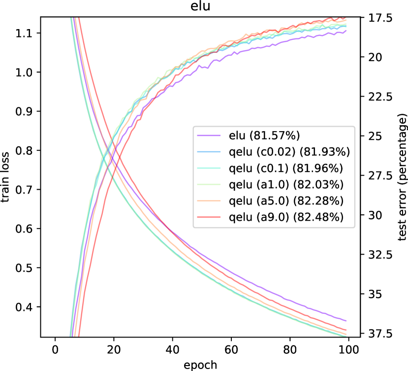
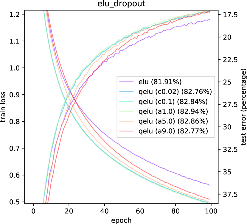
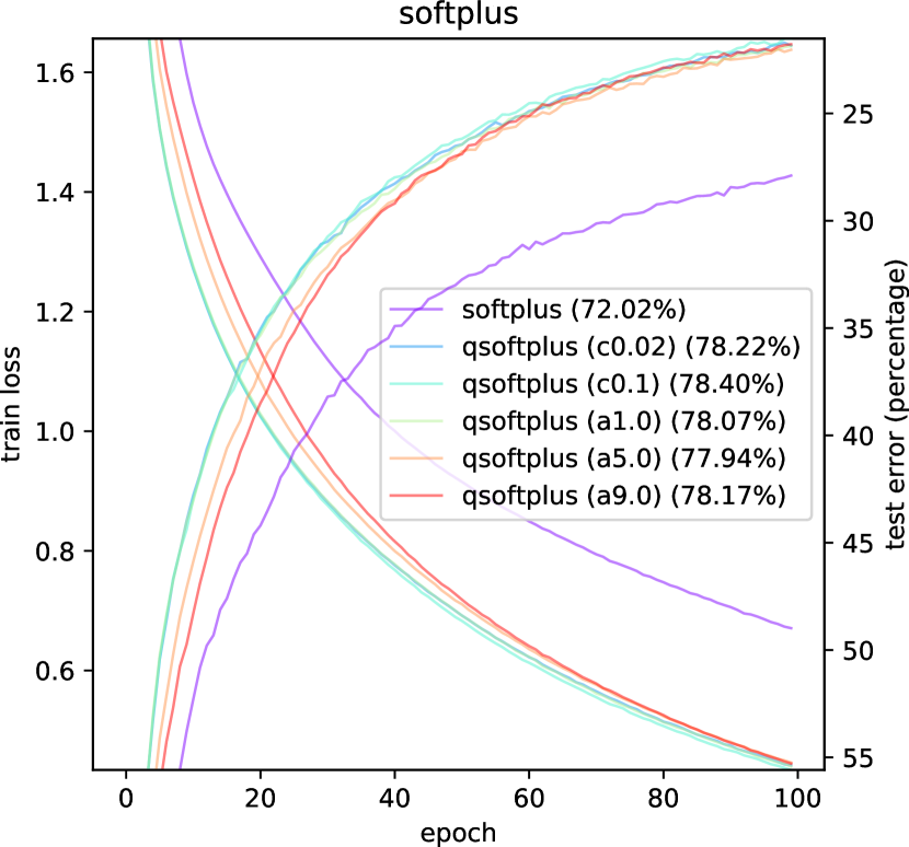
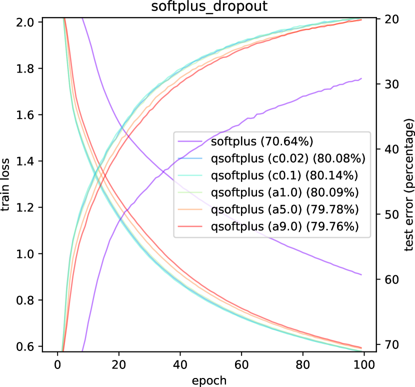
Figure 5: Training loss (descending curves) and testing accuracy (ascending curves) of a CNN on CIFAR10.

4 Conclusion

We proposed the stochastic $q$-neurons based on converting activation functions into corresponding stochastic $q$-activation functions using Jackson’s $q$-calculus. We found experimentally that $q$-neurons can consistently (although slightly) improve the generalization performance, and can goes deeper in the error surface.

Appendix A Brief overview of the $(p,q)$-differential calculus

For $p,q\in\mathbb{R},p\not=q$, define the $(p,q)$-differential:

$$d_{p,q}f(x):=f(qx)-f(px).$$

In particular, $d_{p,q}x=(q-p)x$.

The $(p,q)$-derivative is then obtained as:

$$D_{p,q}f(x):=\frac{d_{p,q}f(x)}{d_{p,q}x}=\frac{f(qx)-f(px)}{(q-p)x}.$$

We have $D_{p,q}f(x)=D_{q,p}f(x)$.

Consider a real-valued scalar function $f(x)$. The differential operator $D$ consists in taking the derivative: $Df(x)=\frac{d}{\mathrm{d}x}=f^{\prime}(x)$.

The $(p,q)$-differential operator $D_{p,q}$ for two distinct scalars $p$ and $q$ is defined by taking the following finite difference ratio:

$$D_{p,q}f(x):=\left\{\begin{array}[]{ll}\frac{f(px)-f(qx)}{(p-q)x},&x\not=0\mbox{\ and\ }p\not=q,\\ f^{\prime}(0),&x=0\mbox{\ or\ }p=q.\end{array}\right.$$ (8)

We have $D_{p,q}f(x)=D_{q,p}f(x)$.

The $(p,q)$-derivative is an extension of Jackson’s $q$-derivative [1, 2, 7, 8] historically introduced in 1909. Notice that this finite difference differential operator that does not require to compute limits (a useful property for derivative-free optimization), and moreover can be applied even to nondifferentiable (e.g., ReLU) or discontinuous functions.

An important property of the $(p,q)$-derivative is that it generalizes the ordinary derivative:

Lemma 3.

For a twice continuously differentiable function $f$, we have $\lim_{p\rightarrow q}D_{p,q}f(x)=\frac{1}{q}Df(qx)=\frac{1}{q}f^{\prime}(qx)$ and $\lim_{x\rightarrow 0}D_{p,q}f(x)=Df(0)=f^{\prime}(0)$.

Proof.

Let us write the first-order Taylor expansion of $f$ with exact Lagrange remainder for a twice continuously differentiable function $f$:

$$f(qx)=f(px)+(qx-px)f^{\prime}(px)+\frac{1}{2}(qx-px)^{2}f^{\prime\prime}(\varepsilon),$$

for $\varepsilon\in(\min\{px,qx\},\max\{px,qx\})$.

It follows that

$$D_{p,q}f(x) = \frac{f(px)-f(qx)}{x(p-q)}=\frac{f(qx)-f(px)}{x(q-p)},$$ (9)

$$= f^{\prime}(px)+\frac{1}{2}x(q-p)f^{\prime\prime}(\varepsilon).$$ (10)

Thus, whenever $p=q$ we have $D_{p,q}f(x)=f^{\prime}(px)=\frac{1}{p}Df(px)$, and whenever $x=0$, we have $D_{p,q}f(0)=f^{\prime}(0)$. In particular, when $p=1$, we have $D_{q}f(x)=f^{\prime}(x)$ when $q=1$ or when $x=0$. ∎

Let us denote $D_{q}$ the $q$-differential operator $D_{q}:=D_{1,q}=D_{q,1}$.

Since $B_{F}(qx:px):=f(qx)-f(px)-(qx-px)f^{\prime}(px)=\frac{1}{2}(qx-px)^{2}f^{\prime\prime}(\varepsilon)$, we can further express the $(p,q)$-differential operator using Bregman divergences [9] as follows:

Corollary 4.

We have:

$$D_{p,q}f(x) = \frac{f(px)-f(qx)}{x(p-q)}=f^{\prime}(px)+\frac{B_{F}(qx:px)}{x(p-q)},$$

$$= \frac{f(qx)-f(px)}{x(q-p)}=f^{\prime}(qx)+\frac{B_{F}(px:qx)}{x(q-p)}.$$

A.1 Leibniz $(p,q)$-rules of differentiation

The following $(p,q)$-Leibniz rules hold:

• Sum rule (linear operator):

  $$D_{p,q}(f(x)+\lambda g(x))=D_{p,q}f(x)+\lambda D_{p,q}g(x)$$

• Product rule:

  $$D_{p,q}(f(x)g(x)) = f(px)+D_{p,q}g(x)+g(qx)D_{p,q}f(x),$$

  $$= f(qx)+D_{p,q}g(x)+g(px)D_{p,q}f(x).$$

• Ratio rule:

  $$D_{p,q}(f(x)/g(x)) = \frac{g(qx)D_{p,q}f(x)-f(qx)D_{p,q}g(x)}{g(px)g(qx)},$$

  $$= \frac{g(px)D_{p,q}f(x)-f(px)D_{p,q}g(x)}{g(px)g(qx)}.$$

A.2 The $(p,q)$-gradient operator

For a multivariate function $F(x)=F(x_{1},\ldots,x_{d})$ with $x=(x_{1},\ldots,x_{d})$, let us define the first-order partial derivatives for $i\in[d]$ and $p_{i}\not=q_{i}$,

$$D_{p,q,x_{i}}F(x) := \left\{\begin{array}[]{ll}\frac{F(x_{1},\ldots,p_{i}x_{i},\ldots,x_{n})-F(x_{1},\ldots,q_{i}x_{i},\ldots,x_{n})}{(p_{i}-q_{i})x_{i}}&x_{i}\not=0,\\ \frac{\partial F(x)}{\partial x_{i}}&x_{i}=0\end{array}\right.$$

$$= \left\{\begin{array}[]{ll}\frac{F(x+(p_{i}-1)e_{i})-F(x+(q_{i}-1)e_{i})}{(p_{i}-q_{i})x_{i}}&x_{i}\not=0,\\ \frac{\partial F(x)}{\partial x_{i}}&x_{i}=0\end{array}\right.,$$

where $e_{i}$ is a one-hot vector with the $i$-th coordinate at one, and all other coordinates at zero.

The generalization of the $(p,q)$-gradient [10] follows by taking $d$-dimensional vectors for $p=(p_{1},\ldots,p_{d})$ and $q=(q_{1},\ldots,q_{d})$:

$$\nabla_{p,q}F(x):=\left[\begin{array}[]{c}D_{p_{1},q_{1},x_{1}}F(x)\\ \vdots\\ D_{p_{d},q_{d},x_{d}}F(x)\end{array}\right]$$

The $(p,q)$-gradient is a linear operator: $\nabla_{p,q}(aF(x)+bG(x))=a\nabla_{p,q}F(x)+b\nabla_{p,q}G(x)$ for any constants $a$ and $b$. When $p,q\rightarrow 1$, $\nabla_{p,q}\rightarrow\nabla$: That is, the $(p,q)$-gradient operator extends the ordinary gradient operator.

A.3 Code snippet in Python

We can easily implement $q$-neurons based on the following reference code, which is based on a given activation function activate. Note, q has the same shape as x. One can fix eps$=10^{-3}$ and only has to tune the hyper-parameter lambda.

def qactivate( x, lambda, eps ):
    q = random_normal( shape=shape(x) )
    q = ( 2*( q>=0 )-1 ) * ( lambda * abs(q) + eps )
    return ( activate( x * (1+q) ) - activate( x ) ) / q

References

- [1] Frank Hilton Jackson, “On -functions and a certain difference operator,” Earth and Environmental Science Transactions of The Royal Society of Edinburgh, vol. 46, no. 2, pp. 253–281, 1909.
- [2] Victor Kac and Pokman Cheung, Quantum Calculus, Universitext. Springer New York, 2001.
- [3] Shujaat Khan, Alishba Sadiq, Imran Naseem, Roberto Togneri, and Mohammed Bennamoun, “Enhanced -least mean square,” 2018, arXiv:1801.00410 [math.OC].
- [4] Érica J. C. Gouvêa, Rommel G. Regis, Aline C. Soterroni, Marluce C. Scarabello, and Fernando M. Ramos, “Global optimization using -gradients,” European Journal of Operational Research, vol. 251, no. 3, pp. 727–738, 2016.
- [5] Andrew L. Maas, Awni Y. Hannun, and Andrew Y. Ng, “Rectifier non-linearities improve neural network acoustic models,” in ICML, 2013.
- [6] Djork-Arné Clevert, Thomas Unterthiner, and Sepp Hochreiter, “Fast and accurate deep network learning by exponential linear units (ELUs),” in ICLR, 2016, arXiv 1511.07289.
- [7] Thomas Ernst, A comprehensive treatment of -calculus, Springer Science & Business Media, 2012.
- [8] Patrick Njionou Sadjang, “On the fundamental theorem of -calculus and some -Taylor formulas,” arXiv preprint arXiv:1309.3934, 2013.
- [9] Arindam Banerjee, Srujana Merugu, Inderjit S Dhillon, and Joydeep Ghosh, “Clustering with Bregman divergences,” Journal of machine learning research, vol. 6, no. Oct, pp. 1705–1749, 2005.
- [10] Aline C. Soterroni, Roberto L. Galski, and Fernando M. Ramos, “The -gradient method for continuous global optimization,” in AIP Conference Proceedings. AIP, 2013, vol. 1558, pp. 2389–2393.
- [11] Zhen Xu and Frank Nielsen, “Beyond Ordinary Stochastic Gradient Descent,” preprint INF517, Ecole Polytechnique, March 2018.
- [12] Arvind Neelakantan, Luke Vilnis, Quoc V. Le, Ilya Sutskever, Lukasz Kaiser, Karol Kurach and James Martens, “Adding Gradient Noise Improves Learning for Very Deep Networks,” in ICLR, 2016, arXiv 1511.06807.
- [13] Nitish Srivastava, Geoffrey Hinton, Alex Krizhevsky, Ilya Sutskever and Ruslan Salakhutdinov, “Dropout: A Simple Way to Prevent Neural Networks from Overfitting,” Journal of machine learning research, vol. 15, no. Jun, pp. 1929–1958, 2014.