Gravitational collapse and formation of universal horizons in Einstein-æther theory

Abstract

We numerically study the gravitational collapse of a massless scalar field with spherical symmetry in Einstein-æther theory, and show that apparent, spin-0 and dynamical universal horizons (dUHs) can be all formed. The spacetime and the æther field are well-behaved and regular, including regions nearby these horizons (but away from the center of spherical symmetry). The spacetime outside the apparent and spin-0 horizons settles down to a static configuration, and some of such resulting static black holes were already found numerically in the literature. On the other hand, the proper distance of the outermost dUH from the apparent (or spin-0) horizon keeps increasing on æther-orthogonal time slices. This indicates that the outermost dUH is evolving into the causal boundary, even for excitations with large speeds of propagation.

I Introduction

Lorentz invariance (LI) is one of the fundamental symmetries of modern physics and strongly supported by observations KR11 . In fact, the experiments carried out so far are all consistent with it, and there is no observational evidence to show that such a symmetry must be broken at certain energy scales, although constraints of such violations in the gravitational sector are much weaker than those in the matter sector Mattingly05 .

There are still various reasons to construct gravitational theories with broken LI. In particular, if space and time are quantized at the Planck scale, as we understand from the point of view of quantum gravity Kiefer12 , then LI cannot be a fundamental continuous symmetry, but instead should be an emergent one at low energies. Another motivation comes from modification of gravity at long distances to explain the accelerated expansion of the late-time universe. Following these lines of argument, Lorentz violating (LV) theories of gravity have attracted lots of interest in recent years. These include ghost condensation ArkaniHamed:2003uy , Einstein-æther theory (æ-theory) Jacobson and Hořava gravity Horava .

However, once LI is broken, different species of particles can travel with different (sometimes arbitrarily large) speeds. This suggests that black holes may exist only at low energies. At high energies, signals with sufficiently large speeds initially emanated inside an event horizon (EH) can escape to infinity. However, in contrast to this physical intuition, it was found that there still exist absolute causal boundaries, the so-called universal horizons (UHs), and particles even with infinitely large velocities would just move along these boundaries and cannot escape to infinity BS11 ; BJS11 ; BBM12 . This is closely related to the causality in LV theories of gravity. Since now the speeds of particles can be arbitrarily large, similar to Newton’s theory, to preserve the causality, it is necessary to introduce a scalar field with globally timelike gradient, the so-called khronon, which defines an absolute time, and all particles are assumed to move along its increasing direction, so the causality in the sense of the past and the future is assured (Cf. Fig. 1 in GLLSW ). Then, in asymptotically flat stationary spacetimes, there might exist a surface on which the timelike translation Killing vector becomes orthogonal to the gradient of the khronon (See e.g. Fig. 2 in LSW16 ). Hence, a particle must cross this surface and move inevitably inward (towards the increasing direction of the khronon), once it arrives at it, no matter how large its speed is. This is a one-way membrane, and particles even with infinitely large speed cannot escape from it, once they are trapped inside. So, it acts as an absolute horizon to all particles. UHs have been extensively studied (see e.g. Wang17 and references therein), including their thermodynamics BBM13 ; CLMV ; DWWZ .

In general relativity (GR), it is well known that EHs can be formed from gravitational collapse of realistic matter, which implies that black holes with EHs as their boundaries exist in our Universe. However, in LV theories since particles with speeds larger than that of light exist, such particles can cross them and escape to infinity, even initially they are trapped inside EHs. So, EHs in such theories are no longer the one-way membranes. Instead, now the black hole boundaries are replaced by UHs, as argued above. Therefore, from the same astrophysical considerations as in GR, a key issue is whether UHs can be also formed from gravitational collapse in our Universe SAM14 ; TWSW15 ; BCCS16 . In this paper, we shall address this important issue in the framework of æ-theory, which propagates three kinds of modes, the usual spin-2 graviton plus the spin-1 and spin-0 ones Jacobson . We numerically show the formation of dynamical UHs (dUHs), the generalization of UHs to dynamical spacetimes with spherical symmetry. We also find that the proper distance of the outermost dUH from the apparent (or spin-0) horizon keeps increasing on æther-orthogonal time slices. To our best knowledge, this is the first time to show explicitly that dUHs can be formed from gravitational collapse.

II ${\ae}$-Theory and Spherical Collapse

The fundamental variables of the gravitational sector of æ-theory are $(g_{\mu\nu},u^{\mu},\lambda)$, where $g_{\mu\nu}$ is the spacetime metric with the signatures $(-,+,+,+)$, and $u^{\mu}$ is the aether four-velocity, while $\lambda$ is a Lagrangian multiplier, which guarantees that $u^{\mu}$ is always timelike and has unit norm. The general action of æ-theory takes the form Jacobson , $S=S_{\mbox{\ae}}+S_{m}$, where $S_{\mbox{\ae}}\;(S_{m})$ denotes the action of gravity (matter), given by

$$S_{\mbox{\ae}} = \frac{1}{16\pi G_{\mbox{\ae}}}\int{\sqrt{-g}\;d^{4}x\Big{[}R+{\cal{L}}_{\mbox{\ae}}\left(g_{\mu\nu},u^{\nu},\lambda\right)\Big{]}},$$

$$S_{m} = \int{\sqrt{-g}\;d^{4}x\Big{[}{\cal{L}}_{m}\left(g_{\mu\nu},\psi\right)\Big{]}}.$$ (1)

Here $G_{\mbox{\ae}}$ is related to the Newtonian constant $G_{N}$ CL04 by $G_{N}={G_{\mbox{\ae}}}/{(1-c_{14}/2)}$,with $c_{ij}\equiv c_{i}+c_{j}$ and $c_{ijk}=c_{i}+c_{j}+c_{k}$, and $\psi$ collectively denotes the matter fields. $R$ is the Ricci scalar, and ${\cal{L}}_{\mbox{\ae}}\equiv-M^{\alpha\beta}_{~{}~{}~{}~{}\mu\nu}\left(D_{\alpha}u^{\mu}\right)\left(D_{\beta}u^{\nu}\right)+\lambda\left(g_{\alpha\beta}u^{\alpha}u^{\beta}+1\right)$, where $D_{\mu}$ denotes the covariant derivative of $g_{\mu\nu}$, $M^{\alpha\beta}_{~{}~{}~{}~{}\mu\nu}\equiv c_{1}g^{\alpha\beta}g_{\mu\nu}+c_{2}\delta^{\alpha}_{\mu}\delta^{\beta}_{\nu}+c_{3}\delta^{\alpha}_{\nu}\delta^{\beta}_{\mu}-c_{4}u^{\alpha}u^{\beta}g_{\mu\nu}$, and $c_{i}$’s are four independent dimensionless coupling constants.

Recently, the combination of the gravitational wave GW170817 GW170817 and the gamma-ray burst GRB 170817A GRB170817 events provided a remarkably stringent constraint on the speed of the spin-2 graviton, $-3\times 10^{-15}<c_{T}-1<7\times 10^{-16}$. In æ-theory, this implies $\left|c_{13}\right|<10^{-15}$ JM04 . Together with other observational and theoretical constraints, the parameter space of æ-theory is restricted to the intersection of OMW18 ,

$$\left|c_{13}\right|<10^{-15},\quad 0\leq c_{14}\leq 2.5\times 10^{-5},$$

$$0\leq c_{2}\leq 0.095,\quad c_{4}\leq 0\,.$$ (2)

The variations of the total action with respect to $g_{\mu\nu}$ and $u^{\mu}$ yield

$$R^{\mu\nu}-\frac{1}{2}g_{\mu\nu}R-T^{\mu\nu}_{\mbox{\ae}}=8\pi G_{\mbox{\ae}}T_{m}^{\mu\nu},$$ (3)

$$D_{\alpha}J^{\alpha}_{~{}~{}~{}\mu}+c_{4}a_{\alpha}D_{\mu}u^{\alpha}+\lambda u_{\mu}=0,$$ (4)

while its variation with respect to $\lambda$ yields $u^{\alpha}u_{\alpha}=-1$. Here, $T_{m}^{\mu\nu}$ denotes the matter energy-stress tensor, and $T_{\mbox{\ae}}^{\alpha\beta}\equiv-D_{\mu}\big{[}u^{(\beta}J^{\alpha)\mu}-J^{\mu(\alpha}u^{\beta)}-J^{(\alpha\beta)}u^{\mu}\big{]}-c_{1}\big{[}\left(D_{\mu}u^{\alpha}\right)\left(D^{\mu}u^{\beta}\right)-\left(D^{\alpha}u_{\mu}\right)\left(D^{\beta}u^{\mu}\right)\big{]}+c_{4}a^{\alpha}a^{\beta}+\lambda u^{\alpha}u^{\beta}-\frac{1}{2}g^{\alpha\beta}J^{\delta}_{\;\;\sigma}D_{\delta}u^{\sigma}$, with $J^{\alpha}_{\;\;\;\mu}\equiv M^{\alpha\beta}_{~{}~{}~{}~{}\mu\nu}D_{\beta}u^{\nu}\,$, $a^{\mu}\equiv u^{\alpha}D_{\alpha}u^{\mu}$, $\lambda=u_{\beta}D_{\alpha}J^{\alpha\beta}+c_{4}a^{2}$, and $a^{2}\equiv a_{\lambda}a^{\lambda}$.

Gravitational collapse of a spherical massless scalar field in æ-theory was already studied in some detail GEJ07 ; AGG18 . In particular, it was shown that for two different sets of $c_{i}$’s [given, respectively, by Eqs.(16) and (34) with $c_{1}=0.7$ in GEJ07 , which will be referred as to GEJ1 and GEJ2], both apparent horizons (AHs) and spin-0 horizons (S0Hs) are formed during the collapse GEJ07 , and the configurations finally settle down to the regular static black holes found numerically in EJ06 . For another set of $c_{i}$’s, the collapse instead results in the temporary formation of a white hole horizon AGG18 , although the corresponding static black hole exists BJS11 . It should be noted that neither GEJ1 nor GEJ2 satisfies the constraints (Eq. II).

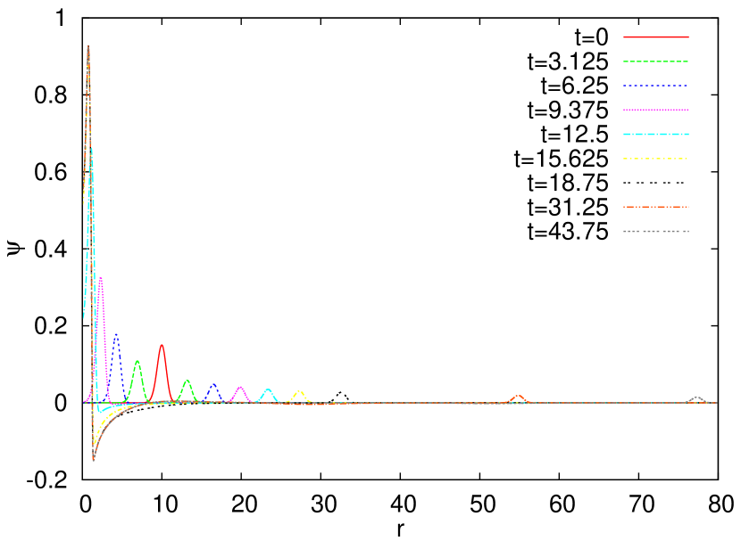
Figure 1: Evolution of the scalar field profile, $\Psi$ for the case GEJ1, using a medium-resolution simulation.

Therefore, in this paper our goals are two-fold: First we show that even within the range of the new constraints, AHs and S0Hs can be still formed from gravitational collapse. Second, dynamical UHs can be also formed. To these goals, we choose to study the same setup as that studied in GEJ07 ; AGG18 , closely following their notation and conventions. This will in particular allow us to check our numerical codes. We choose the surfaces of constant time orthogonal to $u^{\mu}$ and the gauge that leads to the form of metric, $ds^{2}=\gamma_{ab}dx^{a}dx^{b}+\Phi^{2}\left(d\theta^{2}+\sin\theta^{2}d\varphi^{2}\right)$, where $\gamma_{ab}dx^{a}dx^{b}=-\alpha^{2}dt^{2}+\left(dr+\beta^{r}dt\right)^{2}$, $a,b=0,1$; $\alpha,\;\beta^{r}$ and $\Phi$ are functions of $x^{a}=(t,r)$ only; and $u_{\mu}dx^{\mu}=u_{a}dx^{a}=-\alpha dt$, for which the time evolution vector is given by $t^{\mu}=\alpha u^{\mu}+\beta^{\mu}$ with $\beta^{\mu}\partial_{\mu}=\beta^{r}\partial_{r}$. For the massless scalar field $\chi$ we have ${\cal{L}}_{m}=-D_{\nu}\psi D^{\nu}\psi/(16\pi G_{\mbox{\ae}})$, where $\psi\equiv\sqrt{8\pi G_{\mbox{\ae}}}\;\chi$. The evolved quantities are then $(\psi,P,K,a_{r},\Phi)$, where $P\equiv{\cal{L}}_{u}\psi$, and $K$ is the trace of the extrinsic curvature of constant-$t$ surfaces. The dynamical equations and constraints are given, respectively, by GEJ07 ,

$$\dot{\psi} = \alpha P+\beta^{r}\psi^{\prime},$$ (5)

$$\dot{P} = \beta^{r}P^{\prime}+\alpha\left(PK+a^{r}\psi^{\prime}+\psi^{\prime\prime}+\frac{2\Phi^{\prime}}{\Phi}\psi^{\prime}\right),$$ (6)

$$\dot{K} = \beta^{r}K^{\prime}+\frac{\alpha}{3}K^{2}+\frac{\alpha}{\Delta}\Bigg{[}2P^{2}+3\left(1-c_{13}\right)Q^{2}$$ (7)

$$+\left(c_{14}-2\right)\left(a_{r}^{\prime}+2a_{r}\frac{\Phi^{\prime}}{\Phi}+a_{r}^{2}\right)\Bigg{]},$$

$$\dot{a}_{r} = \beta^{r}a_{r}^{\prime}+\alpha\Bigg{[}\left(\frac{2K}{3}-Q\right)a_{r}+\frac{c_{13}}{c_{14}\left(1-c_{13}\right)}P\psi^{\prime}$$ (8)

$$~{}~{}~{}~{}~{}~{}~{}~{}~{}~{}~{}~{}~{}~{}~{}-\frac{c_{123}}{c_{14}\left(1-c_{13}\right)}K^{\prime}\Bigg{]},$$

$$\dot{\Phi} = \beta^{r}\Phi^{\prime}+\alpha\Phi\left(\frac{Q}{2}-\frac{K}{3}\right),$$ (9)

and

$$Q^{\prime} = -3Q\frac{\Phi^{\prime}}{\Phi}+\frac{1}{1-c_{13}}\left(\frac{\Delta}{3}K^{\prime}-P\psi^{\prime}\right),$$ (10)

$$\frac{\alpha^{\prime}}{\alpha} = a_{r},$$ (11)

$${\beta^{r}}^{\prime} = \alpha\left(Q+\frac{K}{3}\right),$$ (12)

$${\cal{C}} = \Phi^{\prime\prime}+\frac{{\Phi^{\prime}}^{2}-1}{2\Phi}+c_{14}a_{r}\Phi^{\prime}+\frac{\Phi}{4}\Bigg{[}c_{14}\left(2a_{r}^{\prime}+a_{r}^{2}\right)$$ (13)

$$+P^{2}+{\psi^{\prime}}^{2}+\frac{3}{2}\left(1-c_{13}\right)Q^{2}-\frac{\Delta}{3}K^{2}\Bigg{]}=0,$$

with $Q\equiv K^{r}_{r}-K/3$, $\Delta\equiv 2+c_{13}+3c_{2}$, $\dot{\psi}\equiv\partial_{t}\psi$, $\psi^{\prime}\equiv\partial_{r}\psi$, and so on.

The locations of the S0Hs and AHs are defined, respectively, by $\tilde{\gamma}^{ab}n_{a}n_{b}=0$ and $\gamma^{ab}n_{a}n_{b}=0$, where $n_{a}\equiv\partial_{a}\Phi$, $\tilde{\gamma}^{ab}=(\tilde{\gamma}^{-1})^{ab}$ and $\tilde{\gamma}_{ab}\equiv\gamma_{ab}+(1-c_{S}^{2})u_{a}u_{b}$ with $c_{S}^{2}\equiv c_{123}(2-c_{14})/[c_{14}(1-c_{13})(2+c_{13}+3c_{2})]$ GEJ07 . Hereafter, by a S0H/AH we shall denote an outer S0H/AH. In stationary spacetimes, UHs are defined by $u_{a}\zeta^{a}=0$, where $\zeta^{a}\partial_{a}$ is the time translation Killing vector BS11 ; Wang17 . However, when spacetimes are dynamical, such a vector does not exist any longer. Following TWSW15 ; Wang17 in defining a dUH, we first introduce the Kodama vector Kodama80 (See also Refs. Hayward:1998ee ; Abreu10 ), $k^{a}\equiv\epsilon^{ab}_{\bot}n_{b}=\left(-\Phi_{,r},\Phi_{,t}\right)/\alpha$, where $\epsilon^{ab}_{\bot}$ is the Levi-Civita tensor with $\epsilon^{01}_{\bot}=-1/\sqrt{-\gamma}$. It is clear that $k^{a}n_{a}=0$. For spacetimes that are asymptotically flat there always exists a region with sufficiently large $\Phi$, in which $n_{a}$ ($k^{a}$) is spacelike (time-like). An AH may form, say, at $r=r_{\text{AH}}$, where $n_{a}$ becomes null. Then, in the trapped region with $\gamma^{ab}n_{a}n_{b}<0$, $n_{a}\;(k^{a})$ becomes timelike (spacelike). We define the location of a dUH as the surface at which

$$u_{a}k^{a}=0,$$ (14)

where in the current case $u_{a}k^{a}=\Phi_{,r}$. Since $u_{a}$ is globally timelike, Eq.(14) is possible only when $k^{a}$ is spacelike. Clearly, this can be true only inside AH, that is, we must have $r_{\text{dUH}}<r_{\text{AH}}$. Eq.(14) may have multiple roots, and what is relevant is the outermost dUH, i.e. the one with the largest $r$ (but not necessarily with the largest $\Phi$). For the outermost dUH, we have ${\Phi}_{\text{dUH}}<{\Phi}_{\text{AH}}$ since $\Phi_{,r}>0$ for $r>r_{\text{dUH}}$. In the stationary spacetimes, the Kodama vector coincides with the time translation vector, and the above definition reduces to static spacetimes, and later generalized to various stationary spacetimes (See Wang17 and references therein).

III Numerical Setup and Results

Our simulations are performed with a finite-differencing code. The initial data, numerical schemes and boundary conditions used in our code also closely follow GEJ07 . The set of PDEs are solved on a uniformly spaced $r$-domain, where $r$ is the proper radial coordinate spanning $[0,r_{\text{max}}],\quad r_{\text{max}}=80$ (or $=320$) with a spacing of $\Delta r=0.003125,0.00625,0.0125$, the high, medium and low resolutions, respectively. The timestep size is set to $0.2\times\Delta r$. In our code, the dynamical variables are integrated in time using an iterated Crank-Nicholson scheme with two iterations. We apply the 4th-order Kreiss-Oliger dissipation with an amplitude of $0.9$ to the time-integration equations so as to damp out spurious high-frequency unstable modes of the solution. The non-dynamical variables $Q$, $\alpha$ and $\beta^{r}$ are integrated through the $r$-domain at every time step using the trapezoidal method. The integration for $\alpha$ is done from $r=r_{\text{max}}$, whereas that for $Q$ and $\beta^{r}$ are done from $r=0$. Specifically, for smoothness we assume $Q$ to be an even function of $r$ and vanish at $r=0$, and $\beta^{r}$ an odd function of $r$. The boundary conditions for both dynamical and non-dynamical variables are imposed at every time step. We shall choose three sets of $c_{i}$’s, GEJ1, GEJ2, and NC, where NC denotes the choice, $c_{13}=0,\;c_{2}=2c_{14}=2.0\times 10^{-7}$, which satisfies the constraints of Eq.(II). For all three sets, the aether field is stable throughout and beyond the collapse of the scalar field to the central region. During the collapsing process, our code converges in a 2nd-order manner in line with the designed order of convergence of the numerical schemes. We further validate our code by reproducing the results of GEJ07 for the parameter sets of GEJ1 and GEJ2. Different boundary conditions for $Q$ and $\beta^{r}$ at $r=0$ or $r=\Delta r$ are tested, and we find that different boundary treatments do not affect the behavior of the PDE system in the bulk of the $r$-domain. In our simulations for all the cases, the scalar field splits into two pieces, with one collapsing under its self-gravity toward $r=0$ and the other traveling to $r\to\infty$ (Fig. 1). As the collapsing piece reaches the central region, we see the formation of the apparent, spin-0 and dynamical universal horizons at finite areal radii.

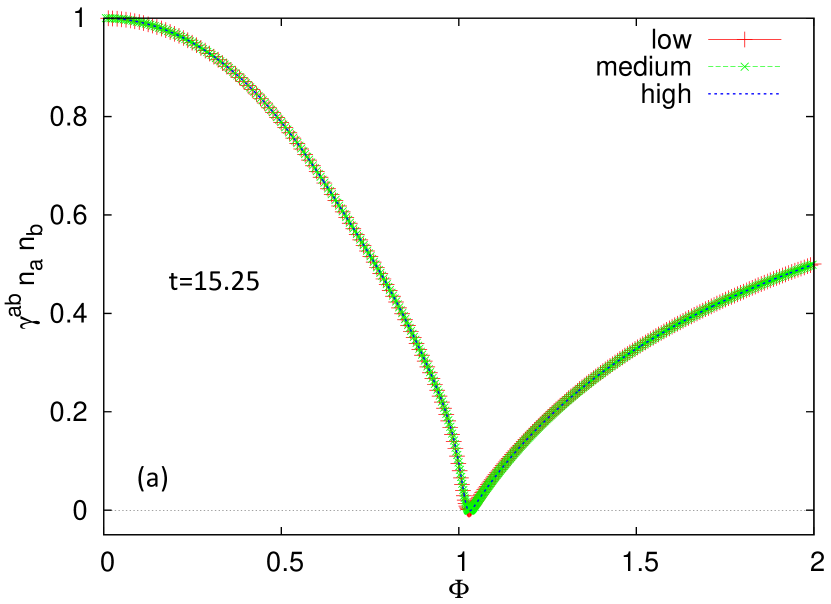
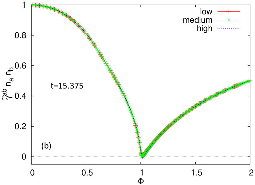
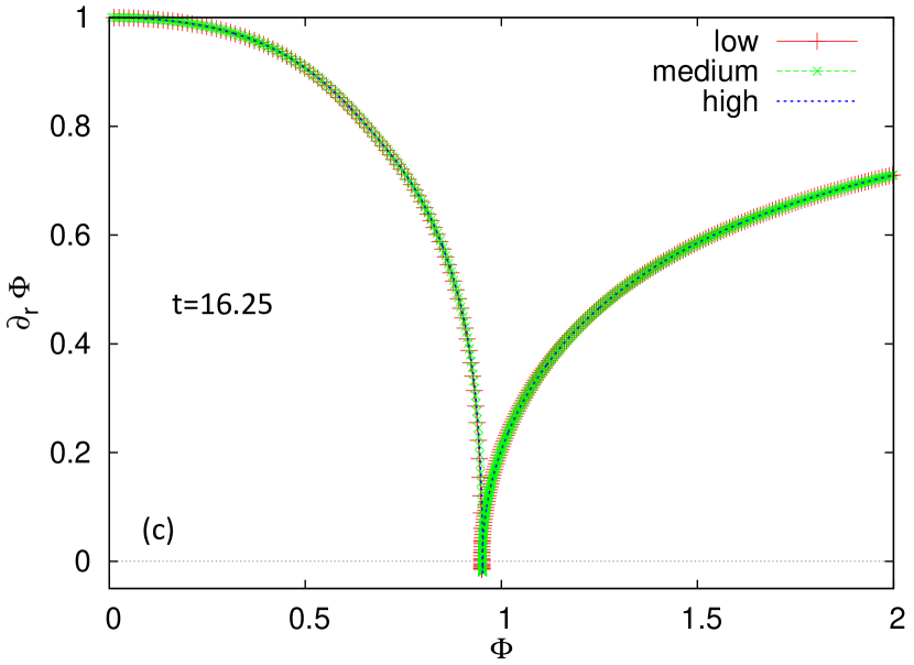
Figure 2: Formation of (a) AH, (b) S0H, and (c) dUH for GEJ1 at the respective times indicated in each panel. The almost complete overlap of the curves obtained from simulations with low, medium and high resolutions show that the system has almost completely converged at the low resolution of this study.

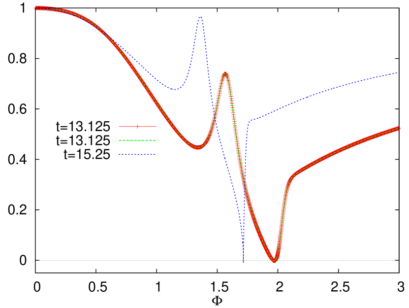
Figure 3: Formation of AH, S0H and dUH for GEJ2 at the respective times indicated in the legend. The red line with crosses represents the profile for $\gamma^{ab}n_{a}n_{b}$, the dashed green line for $\tilde{\gamma}^{ab}n_{a}n_{b}$, and the dashed blue line for $\partial_{r}\Phi$.

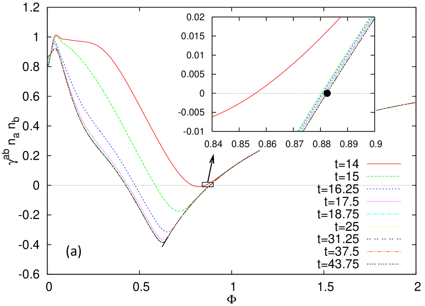
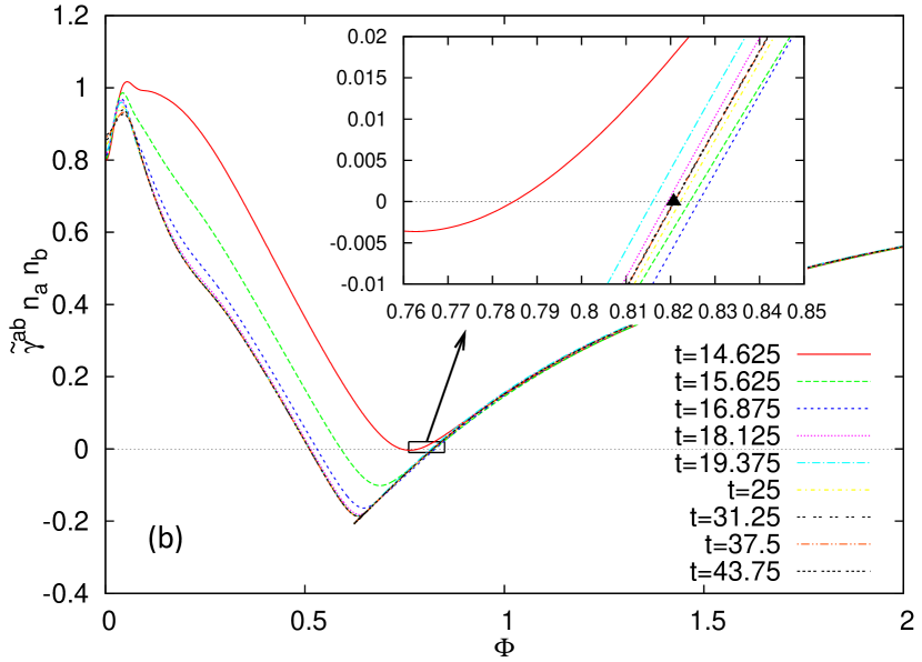
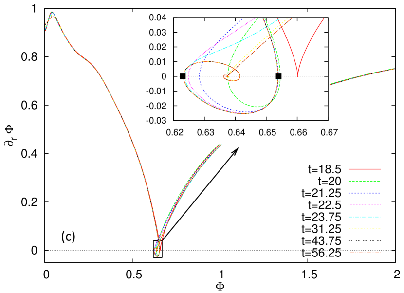
Figure 4: Locations of (a) AH (black dot in inset), (b) S0H (black triangle in inset), and (c) dUHs (black squares in inset) for NC. The red line in each plot indicates the profiles shortly after the respective horizons form.

Fig. 2 shows the profiles of $\gamma^{ab}n_{a}n_{b}$, $\tilde{\gamma}^{ab}n_{a}n_{b}$ and $u_{a}k^{a}(=\partial_{r}\Phi)$ of GEJ1 shortly after the respective horizons are formed. The finite areal radii of these horizons are robust with respect to the resolutions used in this study, indicating that the system has almost completely converged at $\Delta r=0.0125$, i.e., the low resolution (Fig. 2). From tests carried out using $r_{\text{max}}=80,320$ at the medium resolution, we also see that the results are robust with respect to the size of the $r$-domain. At $t=16.25$, a dUH forms at $r\approx 1.40\;(\Phi\approx 0.95)$.

For GEJ2, we track the collapsing process using our high-resolution simulation and similarly find the formation of all three horizons (Fig. 3). As noted in GEJ07 , the AH and S0H in this case coincide since $c_{S}^{2}=1$ and thus $\tilde{\gamma}^{ab}=\gamma^{ab}$. Hereafter, all results are obtained using high-resolution simulations, except for those with $r_{max}=320$.

For NC, the AH forms at $t\approx 14$ and becomes quasi-stationary beginning at $t\approx 25$ with $\Phi\approx 0.8818$ (Fig. 4a). The S0H forms at $t\approx 14.625$ and achieves quasi-stationarity from $t\approx 31.25$ with $\Phi\approx 0.8210$ (Fig. 4b). At $t\approx 18.5$, a dUH forms as a double root of $\partial_{r}\Phi$ at $\Phi\approx 0.660\;(r\approx 2.0)$ (Fig. 4c). After that, the double root splits into two single roots, i.e. the inner (smaller $r$, larger $\Phi$) and outer (larger $r$, smaller $\Phi$) dUHs, and then the areal radius of the outer dUH decreases until it becomes almost constant at $t\approx 31.25$ with $\Phi\approx 0.6232$. The areal radius of the inner dUH becomes almost constant already at $t\approx 21.25$ with $\Phi\approx 0.6538$. At $t\approx 28.69$, an additional pair of dUHs forms outside the already existing pair and thus one of the new pair of dUHs becomes the outermost dUH. The areal radii of the new pair are between those of the old pair. At $t\approx 40.25$, one more pair of dUHs forms outside the two pairs and thus one of the newest pair becomes the outermost dUH. The areal radii of the newest pair are between those of the second pair (Fig. 4c). As time increases, the number of such pairs of dUHs keeps increasing, and one of the newest pair becomes the outermost dUH. This demonstrates that even after the first pair of dUHs (denoted by the two black squares in Fig. 3(c)) has become stationary, the region outside i.e. with larger $r$ (but with $\Phi$’s between the first pair of dUHs) is still highly dynamical. It is interesting to note that static black holes (in the decoupling limit) also have infinite layers of UHs BS11 .

In Fig. 5, we show some physical quantities nearby the locations of the dUHs. While their magnitudes are much higher than those in the surrounding regions, they do not exhibit any blow-up in time, indicating that the spacetime is regular at the locations of these horizons. We note that since we have imposed the smoothness condition at $r=0$, our simulations do not show any blow-up of the curvature at $r=0$.

Using the result of the medium-resolution simulation with $r_{\text{max}}=320$, we plot the change in the proper distance of the outermost dUH from both AH and S0H in Fig. 6. The fact that these distances become longer and longer as time progresses indicates that the outermost dUH is evolving into the causal boundary, even for excitations with large speeds of propagation.

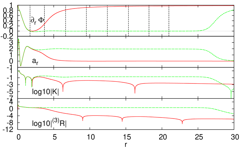
Figure 5: Some physical quantities vs $r$ at $t=18.5$ (solid red line) and $t=56.25$ (dashed green line) for NC. The dashed black vertical lines in the top-most panel indicate the locations of various dUHs at $t=56.25$.

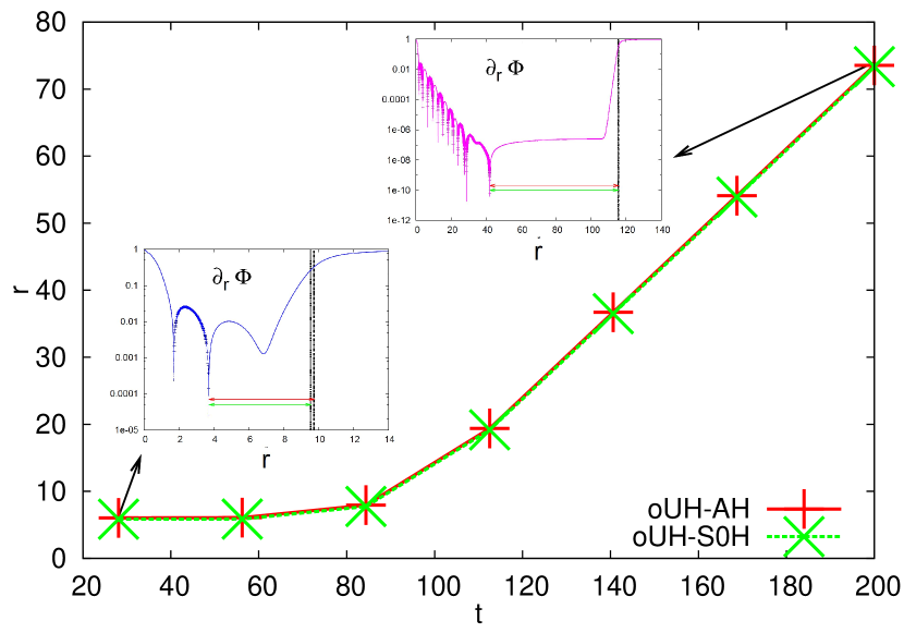
Figure 6: Proper distance $r$ of the outermost dUH from AH labeled by oUH-AH and that from S0H labeled by oUH-S0H for NC.

IV Conclusions

In GR, EHs can be formed from gravitational collapse of realistic matter, so it strongly suggests that black holes with EHs as their boundaries exist in our Universe. However, in gravitational theories with breaking Lorentz symmetry, particles with speeds larger than that of light exist, so those EHs are no longer the one-way membranes to such particles, as they can cross those boundaries and escape to infinity, even initially they are trapped inside them. Instead, now the black hole boundaries are defined by UHs. Therefore, astrophysically it is important to show UHs can be also formed from gravitational collapse of realistic matter, so even with respect to these particles black holes also exist in our Universe SAM14 ; TWSW15 ; BCCS16 .

In this paper, we have numerically studied the gravitational collapse of a massless scalar field with spherical symmetry in $\ae$-theory, and shown explicitly that all three kinds of horizons, apparent, spin-0 and dynamical universal, can be formed from gravitational collapse, by considering three representative sets, GEJ1, GEJ2, and NC, of the free parameters $c_{i}$’s. In the cases of GEJ1 and GEJ2, the collapse finally settles down to the regular static black holes found numerically in EJ06 , although none of these two cases satisfies the constraints of Eq.(II). Also in the case of NC, which satisfies Eq.(II), all three kinds of horizons are formed, and the spacetime in the neighborhoods of these horizons is well-behaved and regular, while the spacetime outside the apparent and spin-0 horizons soon settles down to a static configuration.

Acknowlodgements

We would like to thank D. Garfinkle and S. Sibiryakov for valuable suggestions and comments. S.M. thanks Baylor University for hospitality. This work is supported in part by the National Natural Science Foundation of China (NNSFC), Grant Nos. 11375153 and 11675145. The work of S.M. is supported by JSPS KAKENHI Grant Nos. JP17H02890, JP17H06359, and by WPI, MEXT, Japan.

References

- (1) A. Kostelecky and N. Russell, Rev. Mod. Phys. 83 (2011) 11 [arXiv:0801.0287v7, January 2014 Edition].
- (2) D. Mattingly, Living Rev. Relativity, 8, 5 (2005); S. Liberati, Class. Qnatum Grav. 30, 133001 (2013).
- (3) C. Kiefer, Quantum Gravity, third edition (Oxford Science Publications, Oxford University Press, 2012).
- (4) N. Arkani-Hamed, H. C. Cheng, M. A. Luty and S. Mukohyama, JHEP 0405, 074 (2004).
- (5) T. Jacobson and D. Mattingly, Phys. Rev. D64, 024028 (2001); T. Jacobson, arXiv:0801.1547.
- (6) P. Hořava, Phys. Rev. D79, 084008 (2009).
- (7) S. Sibiryakov, a talk given at the Peyresq 15 meeting, June, 2010; D. Blas and S. Sibiryakov, Phys. Rev. D84, 124043 (2011).
- (8) E. Barausse, T. Jacobson and T. P. Sotiriou, Phys. Rev. D83, 124043 (2011).
- (9) P. Berglund, J. Bhattacharyya and D. Mattingly, Phys. Rev. D85, 124019 (2012).
- (10) J. Greenwald, J. Lenells, J.X. Lu, V.H. Satheeshkumar and A. Wang, Phys. Rev. D84, 084040 (2011).
- (11) K. Lin, V. H. Satheeshkumar, and A. Wang, Phys. Rev. D93, 124025 (2016).
- (12) A. Wang, Int. J. Mod. Phys. D26, 1730014 (2017).
- (13) P. Berglund, J. Bhattacharyya and D. Mattingly, Phys. Rev. Lett. 110, 071301 (2013).
- (14) B. Cropp, S. Liberati, A. Mohd, and V. Matt Visser, Phys. Rev. D89, 064061 (2014).
- (15) C. Ding, A. Wang, and X. Wang, and T. Zhu, Nucl. Phys. B913, 694 (2016).
- (16) M. Saravani, N. Afshordi, and R.B. Mann, Phys. Rev. D89, 084029 (2014).
- (17) M. Tian, X.-W. Wang, M.F. da Silva, and A. Wang, arXiv:1501.04134; M. Tian, X.-W. Wang, M.F. da Silva, S. Mukohyama, and A. Wang, (in preparation).
- (18) J. Bhattacharyya, A. Coates, M. Colombo, and T.P. Sotiriou, Phys. Rev. D93, 064056 (2016).
- (19) J. W. Elliott, G. D. Moore and H. Stoica, JHEP 0508, 066 (2005).
- (20) S. M. Carroll and E. A. Lim, Phys. Rev. D70, 123525 (2004).
- (21) B. Abbott et. al. (Virgo, LIGO Scientific Collaboration), Phys. Rev. Lett. 119, 161101 (2017).
- (22) B. P. Abbott et. al., Virgo, Fermi-GBM, INTEGRAL, LIGO Scientific Collaboration, Astrophys. J. 848 (2017) L13.
- (23) T. Jacobson and D. Mattingly, Phys. Rev. D70, 024003 (2004).
- (24) J. Oost, S. Mukohyama, and A. Wang, Phys. Rev. D97, 124023 (2018).
- (25) D. Garfinkle, C. Eling, and T. Jacobson, Phys. Rev. D76, 034003 (2007).
- (26) R. Akhoury, D. Garfinkle, and N. Gupta, Class. Quantum Grav. 35, 035006 (2018).
- (27) C. Eling and T. Jacobson, Class. Quantum Grav. 23, 5643 (2006).
- (28) H. Kodama, Prog. Theor. Phys. 63, 1217 (1980).
- (29) S. A. Hayward, S. Mukohyama and M. C. Ashworth, Phys. Lett. A256, 347 (1999).
- (30) G. Abreu and M. Visser, Phys. Rev. D82, 044027 (2010).