Wall modes in magnetoconvection at high Hartmann numbers

Abstract

Three-dimensional turbulent magnetoconvection at a Rayleigh number of $Ra=10^{7}$ in liquid gallium at a Prandtl number $Pr=0.025$ is studied in a closed square cell for very strong external vertical magnetic fields $B_{0}$ in direct numerical simulations which apply the quasistatic approximation. As $B_{0}$ or equivalently the Hartmann number $Ha$ are increased, the convection flow that is highly turbulent in the absence of magnetic fields crosses the Chandrasekhar linear stability limit for which thermal convection is ceased in an infinitely extended layer and which can be assigned with a critical Hartmann number $Ha_{\rm c}$. Similar to rotating Rayleigh-Bénard convection, our simulations reveal subcritical sidewall modes that maintain a small but finite convective heat transfer for $Ha>Ha_{\rm c}$. We report a detailed analysis of the complex two-layer structure of these wall modes, their extension into the cell interior and a resulting sidewall boundary layer composition that is found to scale with the Shercliff layer thickness.

1 Introduction

The effect of magnetic fields on the turbulent transport of heat and momentum in turbulent convection is relevant for flow problems ranging from astro- and geophysics (Rüdiger et al., 2013; Weiss & Proctor, 2014) to numerous technological applications (Davidson, 2016). Particularly in engineering, they span a wide spectrum including materials processing, steel casting, dendritic solidification in alloys, and blanket design in nuclear fusion technology. The working fluids are then liquid molten metals with small thermal and very small magnetic Prandtl numbers, $Pr$ and $P_{m}$ which relate momentum diffusion to temperature and magnetic field diffusion, respectively. In addition, typically for liquid metal flows, the induced magnetic field $\bm{b}$ is assumed much smaller than the applied field $B_{0}$, which implies small magnetic Reynolds numbers $R_{m}\ll 1$. Therefore, the quasistatic limit of small $R_{m}$ is applicable with simplifications of the full set of magnetohydrodynamic equations (Knaepen & Moreau, 2008; Davidson, 2016). It is actually also the operating point of most laboratory experiments on Rayleigh-Bénard convection (RBC) with external vertical (Cioni et al., 2000; Burr & Müller, 2001; Aurnou & Olson, 2001) or horizontal magnetic fields (Fauve et al., 1981; Tasaka et al., 2016; Vogt et al., 2018). Nakagawa (1955) and Chandrasekhar (1961) showed that a sufficiently strong vertical external magnetic field $B_{0}$ can suppress the onset of Rayleigh-Bénard convection. For the case of free-slip boundaries at the top and bottom plates, the critical Rayleigh number $Ra_{\rm c}$ of the onset of magnetoconvection in a layer, that is heated from below and cooled from above, is given by

$$Ra_{\rm c}=\frac{\pi^{2}+a^{2}}{a^{2}}\left[(\pi^{2}+a^{2})^{2}+\pi^{2}Ha^{2}\right]\,.$$ (1)

Here, $a=kH$ is the dimensionless horizontal normal mode wave number, $H$ the height of the convection layer and $Ha$ the dimensionless Hartmann number which is given by

$$Ha=B_{0}H\sqrt{\frac{\sigma}{\rho\nu}}\,.$$ (2)

The mass density is $\rho$ and the kinematic viscosity $\nu$. Equation (1) is the Chandrasekhar linear stability limit of magnetoconvection and the relation holds also for no-slip boundary conditions at the top and bottom (Chandrasekhar, 1961). An equation similar to (1) can be derived for a RBC layer that rotates about the vertical axis with a constant angular velocity $\Omega_{0}$ – an alternative way to suppress the onset of convection. It is well-known since the experiments in water or oil of Zhong et al. (1991), Ecke et al. (1992), Liu & Ecke (1999), and King et al. (2012) and the linear stability analyses of Goldstein et al. (1993, 1994) that the existence of sidewalls in closed and rotating cylindrical cells can destabilize convection. For recent direct numerical simulations of rotating liquid metal convection flows, we refer additionally to Horn & Schmid (2017). In other words, convection is present for $Ra<Ra_{\rm c}$ in form of subcritical modes attached to the sidewalls which are denoted as wall modes in the following. This result together with the close analogy to rotating RBC sets the motivation for the present study.

We investigate the impact of a strong vertical magnetic field on a liquid metal convection flow in a closed square cell of aspect ratio 4 by a series of three-dimensional DNS. Therefore liquid metal convection at fixed Rayleigh and Prandtl numbers, $Ra=10^{7}$ and $Pr=0.025$, (the flow is highly turbulent in absence of a magnetic field) is driven to cross the Chandrasekhar stability limit (1) by a stepwise increase of $B_{0}$. The linear stability limit is reached at $Ha_{\rm c}\approx\sqrt{Ra}/\pi\approx 1000$ for the chosen $Ra$ and $Pr$. Our numerical studies show that convective heat transfer is still present for Hartmann numbers up to $Ha=2Ha_{\rm c}$. We also demonstrate by a scale-refined analysis in concentric subvolumes that the transport of heat and momentum is maintained by subcritical flow modes which are attached to the sidewalls, similar to rotating RBC. Furthermore, the spatial organization and structure of these (quasisteady) wall modes is studied in detail. The modes are found here to take the form of circulation rolls that are increasingly closer attached to the sidewalls as $Ha$ grows and form a two-layer boundary flow that scales with the Shercliff thickness, a characteristic boundary scale for a shear flow in a transverse magnetic field (Shercliff, 1953). Wall modes in magnetoconvection were investigated in linear stability analysis by Houchens et al. (2002) in cylindrical cells and predicted by an asymptotic theory along a single straight vertical sidewall between free-slip boundaries at the top and bottom by Busse (2008). Their existence and their complex spatial structure is analysed here for the first time in fully resolved direct numerical simulations of a typical laboratory experiment configuration that starts with fully developed convective turbulence at high Rayleigh number.

2 Numerical model

We solve the three-dimensional equations of magnetoconvection in a closed square box, with $x,y$ as horizontal and $z$ as vertical directions, using the quasistatic limit (Zürner et al., 2016). They couple the velocity field ${\bm{u}}$ with the temperature field $T$ and the external magnetic field ${\bm{B}}=B_{0}{\bm{e}}_{z}$. The equations are made dimensionless by using height of the cell $H$, the free-fall velocity $U_{\rm f}=\sqrt{g\alpha\Delta TH}$, the external magnetic field strength $B_{0}$, and the imposed temperature difference $\Delta T=T_{\rm bottom}-T_{\rm top}$. Four dimensionless control parameters are contained: the Rayleigh number $Ra$, the Prandtl number $Pr$, the Hartmann number $Ha$ and the aspect ratio $\Gamma=L/H$ with $L_{x}=L_{y}=L$. The equations are given by

$${\bm{\nabla}}\cdot{\bm{u}} =0\,,$$ (3)

$$\frac{\partial\bm{u}}{\partial t}+(\bm{u}\cdot\bm{\nabla}){\bm{u}} =-\bm{\nabla}p+\sqrt{\frac{Pr}{Ra}}\left[\bm{\nabla}^{2}\bm{u}+Ha^{2}(\bm{j}\times\bm{e}_{z})\right]+T\bm{e}_{z}\,,$$ (4)

$$\frac{\partial T}{\partial t}+(\bm{u}\cdot\bm{\nabla})T =\frac{1}{\sqrt{RaPr}}\bm{\nabla}^{2}T\,,$$ (5)

where $p$ is the pressure field. The Rayleigh number is $Ra=g\alpha\Delta TH^{3}/(\nu\kappa)$ and the Prandtl number $Pr=\nu/\kappa$. The variable $g$ stands for the acceleration due to gravity, $\alpha$ is the thermal expansion coefficient, $\kappa$ the thermal diffusivity, and $\rho$ the mass density. No-slip boundary conditions for the velocity are applied at all walls. The sidewalls are thermally insulated and the top and bottom plates are held fixed at $T=-0.5$ and 0.5, respectively. All walls are in addition perfectly electrically insulating such that the electric current density ${\bm{j}}$ has to form closed field lines inside the cell. Together with the Ohm law, ${\bm{j}}=-\bm{\nabla}\phi+(\bm{u}\times\bm{e}_{z})$ and divergence-free currents ${\bm{\nabla}}\cdot{\bm{j}}=0$, this results in an additional Poisson equation for the electric potential $\phi$ which is given by

$$\bm{\nabla}^{2}\phi=\bm{\nabla}\cdot(\bm{u}\times\bm{e}_{z})\text{ with }{\partial\phi}/{\partial n}=0\,\text{ on the walls}.$$ (6)

This completes the quasistatic magnetoconvection model. The equations are solved by a second-order finite difference method on a non-uniform Cartesian mesh, discussed in detail in Krasnov et al. (2011). Table 1 summarizes the most important parameters of our DNS runs and reports the (turbulent) momentum transfer quantified by the Reynolds number $Re=u_{\rm rms}\sqrt{Ra/Pr}$ with $u_{\rm rms}=\langle u_{x}^{2}+u_{y}^{2}+u_{z}^{2}\rangle_{V,t}^{1/2}$ and (turbulent) heat transfer measured by the Nusselt number $Nu=1+\sqrt{RaPr}\langle u_{z}T\rangle_{V,t}$ with $\langle\cdot\rangle_{V,t}$ being a combined volume and time average (Scheel & Schumacher, 2016). The values of $Re$ and $Nu$ of run 1 are comparable with those from Scheel & Schumacher (2016) for RB convection in mercury at $Pr=0.021$ in a closed cylindrical cell at $\Gamma=1$ where $Nu=10.11\pm 0.05$ and $Re=8450\pm 100$ is reported.

Beside the thermal boundary layer (BL) thickness $\delta_{T}=1/(2Nu)$ and the viscous boundary layer thickness $\delta_{v}=1/(4\sqrt{Re})$, two further BL thicknesses are relevant for the problem at hand. These are the Hartmann layer thickness $\delta_{\text{Ha}}=a_{1}/Ha$ (Hartmann, 1937) at the top and bottom plates and the Shercliff layer thickness $\delta_{\text{Sh}}=a_{2}/\sqrt{Ha}$ (Shercliff, 1953) at the sidewalls. Constants $a_{1}$ and $a_{2}$ are of order ${\cal O}(1)$ and geometry-dependent. For simplicity, we set $a_{1}=a_{2}=1$ for the following. The grid resolution inside the Hartmann and viscous boundary layers is also listed in table 1 by $N_{BL}$.

Run	$Ha$	$Ra/Ra_{\rm c}$	$N_{x}\times N_{y}\times N_{z}$	$Nu$	$Re$	$N_{BL}$	Runtime
1	0	$\infty$	$\;2048\times 2048\times 512\;$	$\;9.75\pm 0.05\;$	$\;7946\pm 19\;$	18	31
2	200	25.33	$\;\;2048\times 2048\times 512\;\;$	$\;\;7.69\pm 0.12\;\;$	$\;\;3532\pm 27\;\;$	29	31
3	500	4.05	$\;\;2048\times 2048\times 512\;\;$	$\;\;4.11\pm 0.05\;\;$	$\;\;1714\pm 15\;\;$	14	31
4	1000	1.01	$\;2048\times 2048\times 512\;$	$\;1.41$	$\;565\pm 1\;$	8	31
5	1500	0.45	$\;2048\times 2048\times 512\;$	$\;1.28$	$\;425$	8	31
6	2000	0.25	$\;2560\times 2560\times 640\;$	$\;1.15$	$\;287$	8	31

Table 1: Parameters of the simulations. The Prandtl number is fixed to $Pr=0.025$, the Rayleigh number to $Ra=10^{7}$, and the aspect ratio to $\Gamma=4$. The Hartmann number $Ha$, the ratio $Ra/Ra_{\rm c}$ with $Ra_{\rm c}\approx\pi^{2}Ha^{2}$ (ratios $Ra/Ra_{\rm c}<1$ imply convection beyond the Chandrasekhar limit), the grid resolution, the Nusselt number $Nu$, the Reynolds number $Re$ are given. We also list the number of horizontal grid planes inside the Hartmann layer with thickness $\delta_{\text{Ha}}$. In case of $Ha=0$, we substitute the Hartmann layer thickness by the viscous boundary layer thickness $\delta_{v}$. Finally, the total runtime is given in free fall time units, $T_{\rm f}=H/U_{\rm f}$.

3 Results

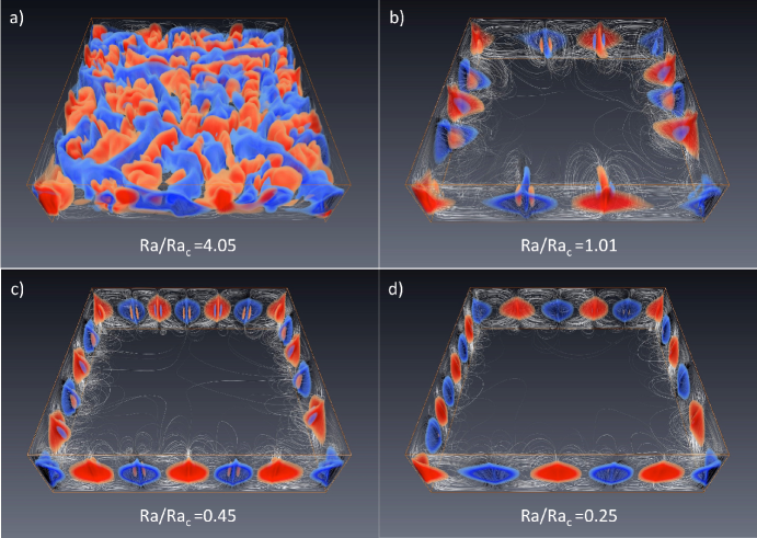
Figure 1: Snapshots of the magnetoconvection flow at (a) $Ha=500$. (b) $Ha=1000$. (c) $Ha=1500$. (d) $Ha=2000$. We display isosurfaces of $u_{z}=\pm 0.01$ together with field lines of the velocity field that highlight the circulation rolls at the sidewalls. The ratio $Ra/Ra_{\rm c}$ is indicated in each of the panels with $Ra_{\rm c}=\pi^{2}Ha^{2}$. For ratios of $Ra/Ra_{\rm c}<1$ the linear stability theory predicts a purely diffusive transport in a fluid layer with ${\bm{u}}=0$.

3.1 Spatial structure of sidewall modes

Figure 1 displays snapshots of the velocity field structure of the magnetoconvection flows. Isosurfaces of the vertical velocity component and field lines of the velocity field are shown for runs at $Ha\geq 500$. For small external magnetic field strength, a cellular structure of up- and downwelling flows is observed that fills the entire cell. A sufficiently strong external magnetic field that corresponds here to $Ha\geq 1000$ expels convective motion from the interior of the cell where heat is then transported solely by diffusion. We note that the critical Hartmann number, which corresponds to the Chandrasekhar linear stability limit, is given by $Ha_{\rm c}=\sqrt{Ra}/\pi\approx 1007$ for the present Rayleigh number of $Ra=10^{7}$. Figures 1(b)–(d) display the structure of the wall modes, which consist of alternating up- and downwelling flow regions attached to the sidewalls. They correspond to neighboring circulation rolls which do not move along the sidewalls or oscillate as in rotating convection for the total integration times that we could run the simulations. The wall modes are ever closer attached to the sidewalls as $Ha$ grows from $1000$ to $2000$. Interestingly, vertical velocity maxima reach out into the bulk in form of tongue-like filaments which might be a relic from the turbulent flow pattern, a point that will be analysed more closely in subsection 3.3.

Figure 2: Global transport of heat and momentum. (a) Nusselt number $Nu$ normalized with respect to the Nusselt number value at $B_{0}=0$ versus $Ha/\sqrt{Ra}$. Present data are given by red filled circles. A part of the data of the experiment by Cioni et al. (2000) is added (open circles). (b) Mean profiles of temperature $T(z)=\langle T(z)\rangle_{A,t}$. (c) Mean profiles of convective heat current, $j_{\rm c}(z)$ (solid lines), and diffusive heat current, $j_{\rm d}(z)$ (dash-dotted lines) for various Hartmann numbers. Both currents are defined in (7). The dotted lines in (c) correspond to $Nu(z)=j_{\rm c}(z)+j_{\rm d}(z)=const.$ (d) Mean profile of the root-mean-square (rms) for the full velocity field (solid line) and the vertical velocity component (dashed line).

3.2 Global and near-sidewall transport of heat and momentum

Table 1 shows that the Nusselt number is still larger unity for runs 4–6 beyond the Chandrasekhar limit. With growing $Ha$ the global transport converges to the pure diffusion case at $Nu=1$. The strong temporal velocity fluctuations of the highly inertial low–$Pr$ turbulence for absent or weak magnetic fields decrease then to vanishingly small values and result in a practically quasisteady laminar wall mode flow. The global analysis of transport is refined in figure 2 by vertical mean profiles taken with respect to horizontal plane $A=\Gamma^{2}$ and time, $\langle\cdot\rangle_{A,t}$. Figure 2(a) compares our Nusselt numbers directly to the experiments in a closed cylinder by Cioni et al. (2000). It can be seen that their data record coincides well the DNS below the Chandrasekhar limit. Deviations are observed for the highest magnetic fields where the data points of the simulation branch off due to the existence of wall modes. Figure 2(b) shows the temperature profiles for all six data sets. The well-mixed bulk region for the turbulent cases at $Ha<1000$ changes to an almost linear diffusion-dominated profile for $Ha\geq 1000$. The Nusselt number is decomposed into two terms that stand for the convective and diffusive heat fluxes across the layer,

$$Nu(z)=j_{\rm c}(z)+j_{\rm d}(z)=\sqrt{RaPr}\,\langle u_{z}T\rangle_{A,t}-\frac{\partial\langle T\rangle_{A,t}}{\partial z}\,.$$ (7)

Figure 2(c) displays the profiles of $j_{\rm c}(z)$ and $j_{\rm d}(z)$ for the three runs with $Ha\geq 1000$ as well as their sum (which has to be constant and equal to $Nu$). It is seen that $j_{\rm d}(z)>j_{\rm c}(z)$. The increasing suppression of fluid turbulence is also demonstrated in figure 2(d) by the root-mean-square (rms) velocity profiles which are given for the quasisteady cases for $Ha\geq 1000$ by $u_{\rm rms}(z)=\langle u_{x}^{2}+u_{y}^{2}+u_{z}^{2}\rangle_{A}^{1/2}$ and $w_{\rm rms}(z)=\langle u_{z}^{2}\rangle_{A}^{1/2}$. It is not only that total fluctuation level decreases then as a whole, but also that the vertical velocity fluctuations provide an increasing fraction to the total fluctuation magnitude for $Ha\geq Ha_{\rm c}$. Furthermore, we find that the ratio of the root mean square values taken in the full cell volume, $w_{\rm rms}/u_{\rm rms}=0.55,0.78,0.90,0.71,0.82$, and 0.83 for the six simulation runs.

The importance of the wall modes for the transport of heat and momentum beyond the Chandrasekhar limit is highlighted in figure 3 where we determine Nusselt number and root mean square velocities over successively smaller concentric cross section areas $S=[r,\Gamma-r]\times[r,\Gamma-r]$ with $r$ being the sidewall-normal distance. These averages are indicated by $\langle\cdot\rangle_{S}$. As visible in figure 3, the transport decreases significantly within a few Shercliff layer thicknesses $\delta_{\text{Sh}}=1/\sqrt{Ha}$ thus further supports the hypothesis that the transport for $Ha>Ha_{\rm c}$ is connected to the wall modes. It is also seen that the heat transfer drops to the diffusive lower bound of $Nu=1$ for $r\gtrsim 2\delta_{\text{Sh}}$ for the highest Hartmann number. All velocity profiles drop significantly towards the center of the cell.

Figure 3: Near-sidewall transport of heat and momentum beyond the Chandrasekhar stability limit. Nusselt number and root mean square velocities are determined over successively smaller horizontal cross section $S$. Profiles are plotted versus a sidewall-normal distance $r$ in units of the Shercliff layer thickness $\delta_{\text{Sh}}$. (a) Nusselt number $\langle Nu\rangle_{S}$. (b) Root mean square velocity $\langle u_{i}^{2}\rangle_{S}^{1/2}$=$\langle u_{x}^{2}+u_{y}^{2}+u_{z}^{2}\rangle_{S}^{1/2}$. (c) Root mean square vertical velocity component $\langle u_{z}^{2}\rangle_{S}^{1/2}$. Data are $Ha=1000,1500$ and 2000 as indicated in the legend in (a).

3.3 Wall-mode structure together with thermal and Shercliff boundary layers

We proceed with an analysis of the viscous and thermal boundary layers in conjunction with the wall-modes. In table 2, we list all important BL thicknesses. The thermal boundary layer thickness $\delta_{T}=1/(2Nu)$ at the top and bottom approaches 0.5 in agreement with $Nu\to 1$ as $Ha$ grows. The mean thermal BL thickness at the sidewall, $\delta_{T}^{\rm(sw)}$ is obtained from profiles of the temperature fluctuations, $\theta({\bm{x}},t)=T({\bm{x}},t)-\langle T(z)\rangle_{A,t}$, with respect to the sidewall-normal coordinate $r$. These profiles are calculated for $Ha\geq 1000$ only, i.e., when the dominantly vertical up- and downflows are attached to the sidewalls. They are always obtained as an average over all four sidewalls. The value of $\delta_{T}^{\rm(sw)}$ is determined by a standard slope method, i.e., as the intersection point of the horizontal line drawn through the mean value of $\langle\theta(r)\rangle_{\rm sw}$ in the bulk and a tangent which is fitted to the same profile very close to the sidewall. The corresponding values decrease as $Ha$ grows and are given in table 2.

In the presence of a strong $B_{0}$, the standard viscous boundary layer thickness $\delta_{v}$ has to be substituted by the Hartmann layer thickness $\delta_{\text{Ha}}=1/Ha$ at the top and bottom. As seen in table 2, the Hartmann layers become extremely thin and their appropriate resolution makes these DNS very demanding. The viscous sidewall layers are also affected by the external magnetic field. Here the fluid motion in horizontal ($x$,$y$)-directions, i.e. transverse to the sidewall-parallel magnetic field, is affected and Shercliff layers with thickness $\delta_{\rm Sh}$ are formed. The Shercliff thickness will be chosen as the length-scale in which the wall modes are measured. The latter ones establish a complex flow structure at the sidewalls which is quantified in figure 4 for the highest external field at $Ha=2000$. We observe the alternating up- and downflows of warmer and colder fluid, respectively (see figure 4(a,b)). The tongue-like structure consists of three thin counter-flowing jets (up-down-upwelling or down-up-downwelling) which arise due to the incompressibility condition (see figures 4(b) and 1). The velocity amplitude inside the modes is still remarkably large with a maximum of $u_{z}\sim 0.1$ as seen in figure 4(d).

Figures 4(b,c) shows a two-layer structure of the wall modes on the basis of the vertical velocity component and heat transport. Figure 5 supports this observation further by an analysis of the convective heat transfer $\langle Nu\rangle_{S}-1=\sqrt{RaPr}\langle u_{z}T\rangle_{S}$ (see also figure 3(a)). For all runs at $Ha\geq 1000$, two exponential decays laws can be observed. These decays separate two different layers: the bulk region dominated by diffusive heat transport and the inner near-wall region with residual convective flow motion, particularly well observable at the highest $Ha=2000$. We have verified that the pronounced minimum at this largest Hartmann number persists for finer computational grids by shorter test reruns at higher resolutions. The crossover distance $r_{\rm cr}$, identified as the intersection point of both exponential fits, is found at a fixed ratio to the Shercliff layer thickness $\delta_{\text{Sh}}$ for the three runs, as given in the table 2. This result implies that the inner section of the sidewall layer is on average of Shercliff-type despite the alternating pattern of horizontal up- and downflows. The distance $r_{\rm cr}$ matches the point where the thin tongue-like vertical flows in figure 4(b,c) appear. Interestingly, the exponential fit $Nu-1\approx A\times\exp(-\beta r)$ of the inner sublayer for $r\leq r_{\rm cr}$ results in spatial decay rates $\beta$ being a fixed ratio to the interaction parameter (or Stuart number) $N=Ha^{2}/\sqrt{Ra/Pr}$. This parameter relates Lorentz to inertial forces and, in the present DNS series, underlines the dominance of Lorentz forces at $Ha\geq 1000$.

Run	$Ha$	$\delta_{T}$	$\delta^{\rm(sw)}_{T}$	$\delta_{\rm Ha}$	$\delta_{\rm Sh}$	$\delta^{\rm(sw)}_{T}/\delta_{\rm Sh}$	$r_{\rm cr}/\delta_{\rm Sh}$	$\beta/N$
1	0	0.051	–	$\infty$	$\infty$	–	–	–
2	200	0.065	–	0.005	$0.071$	–	–	–
3	500	0.122	–	0.002	$0.045$	–	–	–
4	1000	0.355	0.338	0.0010	$0.032$	10.69	3.46	0.30
5	1500	0.391	0.260	0.0007	$0.026$	10.07	3.46	0.30
6	2000	0.435	0.227	0.0005	$0.022$	10.15	3.47	0.30

Table 2: Summarizing list of different boundary layer thicknesses which can be obtained in the magnetoconvection flow in a closed cell. We list thermal BL thicknesses at top/bottom and sidewalls as well as Hartmann and Shercliff layer thicknesses. For the runs with wall modes we also list the ratios $r_{\rm cr}/\delta_{\rm Sh}$ and $\beta/N$ to quantify a two-layer structure. Here, $r_{\rm cr}$ is the crossover width of the two spatial decays laws of convective heat flux of the wall modes. The exponential decay of the inner layer is measured by exponent $\beta$ which is found in a fixed ratio to the corresponding interaction parameter (or Stuart number) $N=Ha^{2}/\sqrt{Ra/Pr}$.

Figure 4: Detailed structure of the wall modes at $Ha=2000$. Horizontal cross section of the time-averaged (a) temperature field $T$, (b) vertical velocity component $u_{z}$ and (c) heat transport $u_{z}T$ at the mid-plane ($z=0$). The violet horizontal line indicates Shercliff boundary layer thickness $\delta_{\rm Sh}$. The green horizontal line indicates $r_{\rm cr}=3.47\delta_{\rm Sh}$. Sidewall distance $r_{\rm cr}$ is determined in figure 5. (d) Profiles of vertical velocity component versus the wall $y$-distance are taken at seven $x$-positions indicated by the cyan vertical lines in panel (b). Profiles from red to blue via grey correspond to the cyan lines from left to right. The vertical velocity component is averaged over the whole cell height in these profiles.

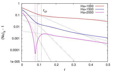
Figure 5: Two-layer structure of the wall modes. The global convective heat flux $Nu-1$ taken over cross sections $S$ is plotted with respect to the sidewall-normal coordinate $r$ is plotted for $Ha\geq 1000$. The spatial exponential decay with $r$ is fitted by two separate scaling laws which intersect at $r=r_{\rm cr}$.

4 Summary and discussion

We have studied three-dimensional magnetoconvection in a closed rectangular cell under the influence of a strong external vertical magnetic field $B_{0}$. An increase of the magnetic field strength, which is measured by an increasing Hartmann number $Ha$, suppresses the highly turbulent motion of the enclosed liquid metal at $B_{0}=0$ ever stronger. In a close analogy to rotating RB convection, we find (laminar) sidewall modes that continue to exist for magnetic fields with $Ha>Ha_{\rm c}$. For the present set of simulations, we were able to follow these wall modes up to $Ha=2Ha_{\rm c}$. A further increase of the Hartmann number would require even finer mesh resolutions at the sidewalls. It is planned to ramp up these simulations for higher Hartmann numbers in the future.

A splitted jet or sandwich-type structure was seen in the linearly unstable modes of Houchens et al. (2002). Our present simulations revealed this double-layer structure of the wall modes and show that it scales with the Shercliff layer thickness. This again is similar to the boundary thicknesses near the sidewall in the rotating convection case where wall modes were found to be related to Stewartson layers that scale with Ekman number (Kunnen et al., 2011, 2013). We did not observe a drift of the wall modes which was observed in rotating RBC with different cell geometries (Knobloch, 1998; Vasil et al., 2008; Horn & Schmid, 2017) and can be traced back to a breaking of azimuthal reflection symmetry (Ecke et al., 1992). It remains open which symmetry-breaking bifurcation could be at work for the convection flow in the presence of a strong magnetic field. The absence of a drift in our DNS might be attributed to the relatively short total integration time of 31 free fall time units which is a small fraction of the momentum diffusion time scale – the slowest time in our flow on the basis of characteristic system parameters. At $Ra=10^{7}$ and $Pr=0.025$ this results to $t_{\rm vis}=\sqrt{Ra/Pr}\,T_{f}=2\times 10^{4}T_{f}$. Indeed, at Hartmann numbers of $Ha\geq 1000$, magnetoconvection becomes a very slow dynamical process and numerical studies would require extremely long-term runs of this order of magnitude.

Our present numerical findings for the existence of wall modes are consistent with the predictions by Houchens et al. (2002) and Busse (2008) for the Hartmann number $\overline{Ha}_{c}$ at which the convection should be completely ceased in a closed cell. For $Ra=10^{7}$, this gives $\overline{Ha}_{c}=(Ra/68.25)^{2/3}\approx 2777$ if the asymptotic solution of Houchens et al. (2002) is taken from their closed cylindrical cell with $\Gamma=1$. From the asymptotic theory of Busse (2008) that applies free-slip boundary conditions at the top and bottom plates follows $\overline{Ha}_{c}=(Ra/(3\pi^{2}\sqrt{3\pi/2}))^{2/3}\approx 2890$. Both theoretical approaches suggest thresholds that are still larger than the Hartmann number which could be obtained here. This should however be possible in a simulations which we plan to conduct in the near future, as already stated.

The observed wall modes resemble also an interesting similarity to isolated turbulent spots in the Shercliff layers in MHD pipe and duct flows at the edge of relaminarization Krasnov et al. (2013); Zikanov et al. (2014). Despite one major difference – the present system is linearly unstable in contrast to pipe and square duct flows – both cases lead to the development of residual structures that maintain a transport of heat and momentum. They are formed in thin near-wall zones, whereas the rest of the domain remains essentially unperturbed. Similar to MHD duct and pipe flows, wall modes are rather weak and, thus, difficult to identify in experiments if only integral parameters can be measured as discussed by Krasnov et al. (2013). Figure 2(b) and table 1 show that these modes provide virtually no impact on the vertical temperature distribution and the Nusselt number only slightly differs from the lower diffusive bound. These similarities suggest that the residual sidewall structures are very likely a common feature of MHD wall bounded flows subject to strong external magnetic fields.

WL is supported by the Deutsche Forschungsgemeinschaft with Grant No. GRK 1567 and by a Fellowship of the China Scholarship Council. DK acknowledges support by the Deutsche Forschungsgemeinschaft with Grant SCHU 1410/29. Computer time has been provided by Large Scale Project pr62se of the Gauss Centre for Supercomputing at the SuperMUC cluster at the Leibniz Rechenzentrum Garching. We thank Till Zürner, André Thess and Christian Karcher for discussions and suggestions. The work of JS is also supported by the Tandon School of Engineering at New York University.

References

- Aurnou & Olson (2001) Aurnou, J. M. & Olson, P. L. 2001 Experiments on Rayleigh-Bénard convection, magnetoconvection and rotating magnetoconvection in liquid gallium. J. Fluid Mech 430, 283–307.
- Burr & Müller (2001) Burr, U. & Müller, U. 2001 Rayleigh-Bénard convection in liquid metal layers under the influence of a vertical magnetic field. Phys. Fluids 13 (11), 3247–3257.
- Busse (2008) Busse, F. H. 2008 Asymptotic theory of wall-attached convection in a horizontal fluid layer with a vertical magnetic field. Phys. Fluids 20 (2), 024102.
- Chandrasekhar (1961) Chandrasekhar, S. 1961 Hydrodynamic and Hydromagnetic Stability. Dover.
- Cioni et al. (2000) Cioni, S., Chaumat, S. & Sommeria, J. 2000 Effect of a vertical magnetic field on turbulent Rayleigh-Bénard convection. Phys. Rev. E 62 (4), R4520.
- Davidson (2016) Davidson, P. A. 2016 Introduction to Magnetohydrodynamics. Cambridge University Press.
- Ecke et al. (1992) Ecke, R. E., Zhong, F. & Knobloch, E. 1992 Hopf bifurcation with broken reflection symmetry in rotating Rayleigh-Bénard convection. Europhys. Lett. 19 (3), 177–182.
- Fauve et al. (1981) Fauve, S., Laroche, C. & Libchaber, A. 1981 Effect of a horizontal magnetic field on convective instabilities in mercury. J. de Phys. Lettres 42 (21), 455–457.
- Goldstein et al. (1993) Goldstein, H. F., Knobloch, E., Mercader, I. & Net, M. 1993 Convection in a rotating cylinder. Part 1. Linear theory for moderate Prandtl numbers. J. Fluid Mech. 248, 583–604.
- Goldstein et al. (1994) Goldstein, H. F., Knobloch, E., Mercader, I. & Net, M. 1994 Convection in a rotating cylinder. Part 2. Linear theory for low Prandtl numbers. J. Fluid Mech. 262, 293–324.
- Hartmann (1937) Hartmann, J. 1937 Hg-dynamics I: theory of the laminar flow of an electrically conductive liquid in a homogeneous magnetic field. K. Dan. Vidensk. Selsk. Mat. Fys. Medd. 15, 1–28.
- Horn & Schmid (2017) Horn, S. & Schmid, P. J. 2017 Prograde, retrograde, and oscillatory modes in rotating Rayleigh–Bénard convection. J. Fluid Mech. 831, 182–211.
- Houchens et al. (2002) Houchens, B. C., Witkowski, L. M. & Walker, J. S. 2002 Rayleigh-Bénard instability in a vertical cylinder with a vertical magnetic field. J. Fluid Mech. 469, 189–207.
- King et al. (2012) King, E. M., Stellmach, S. & Aurnou, J. M. 2012 Heat transfer by rapidly rotating Rayleigh-Bénard convection. J. Fluid Mech. 691, 568–582.
- Knaepen & Moreau (2008) Knaepen, B. & Moreau, R. 2008 Magnetohydrodynamic turbulence at low magnetic Reynolds number. Annu. Rev. Fluid Mech. 40, 25–45.
- Knobloch (1998) Knobloch, E. 1998 Rotating convection: recent developments. Int. J. Eng. Sci. 36 (12), 1421–1450.
- Krasnov et al. (2013) Krasnov, D., Thess, A., Boeck, T., Zhao, Y. & Zikanov, O. 2013 Patterned turbulence in liquid metal flow: Computational reconstruction of the Hartmann experiment. Phys. Rev. Lett. 110, 084501.
- Krasnov et al. (2011) Krasnov, D., Zikanov, O. & Boeck, T. 2011 Comparative study of finite difference approaches in simulation of magnetohydrodynamic turbulence at low magnetic Reynolds number. Comput. Fluids 50 (1), 46–59.
- Kunnen et al. (2013) Kunnen, R. P. J., Clercx, H. J. H. & Van Heijst, G. J. F. 2013 The structure of sidewall boundary layers in confined rotating Rayleigh-Bénard convection. J. Fluid Mech. 727, 509–532.
- Kunnen et al. (2011) Kunnen, R. P. J., Stevens, R. J.A.M., Overkamp, J., Sun, C., Van Heijst, G. J. F. & Clercx, H. J. H. 2011 The role of Stewartson and Ekman layers in turbulent rotating Rayleigh-Bénard convection. J. Fluid Mech. 688, 422–442.
- Liu & Ecke (1999) Liu, Y. & Ecke, R. E. 1999 Nonlinear travelling waves in rotating Rayleigh-Bénard convection: stability boundaries and phase diffusion. Phys. Rev. E 59, 4091–4105.
- Nakagawa (1955) Nakagawa, Y. 1955 An experiment on the inhibition of thermal convection by a magnetic field. Nature 175, 417–419.
- Rüdiger et al. (2013) Rüdiger, G., Kitchatinov, L. L. & Hollerbach, R. 2013 Magnetic Processes in Astrophysics: Theory, Simulations, Experiments. John Wiley & Sons.
- Scheel & Schumacher (2016) Scheel, J. D. & Schumacher, J. 2016 Global and local statistics in turbulent convection at low Prandtl numbers. J. Fluid Mech. 802, 147–173.
- Shercliff (1953) Shercliff, J. A. 1953 Steady motion of conducting fluids in pipes under transverse magnetic fields. Mathematical Proceedings of the Cambridge Philosophical Society 49, 136–144.
- Tasaka et al. (2016) Tasaka, Y., Igaki, K., Yanagisawa, T., Vogt, T., Zürner, T. & Eckert, S. 2016 Regular flow reversals in Rayleigh-Bénard convection in a horizontal magnetic field. Phys. Rev. E 93 (4), 043109.
- Vasil et al. (2008) Vasil, G. M., Brummell, N. H. & Julien, K. 2008 A new method for fast transforms in parity-mixed PDEs: Part II. Application to confined rotating convection. J. Comput. Phys. 227 (17), 8017–8034.
- Vogt et al. (2018) Vogt, T., Ishimi, W., Yanagisawa, T., Tasaka, Y., Sakuraba, A. & Eckert, S. 2018 Transition between quasi-two-dimensional and three-dimensional Rayleigh-Bénard convection in a horizontal magnetic field. Phys. Rev. Fluids 3, 013503.
- Weiss & Proctor (2014) Weiss, N. O. & Proctor, M. R. E. 2014 Magnetoconvection. Cambridge University Press.
- Zhong et al. (1991) Zhong, F., Ecke, R. E. & Steinberg, V. 1991 Asymmetric modes and transition to vortex structures in rotating Rayleigh-Bénard convection. Phys. Rev. Lett. 67, 2473–2476.
- Zikanov et al. (2014) Zikanov, O., Krasnov, D., Boeck, T., Thess, A. & Rossi, M. 2014 Laminar-turbulent transition in magnetohydrodynamic duct, pipe, and channel flows. Appl. Mech. Rev. 66 (3), 030802.
- Zürner et al. (2016) Zürner, T., Liu, W., Krasnov, D. & Schumacher, J. 2016 Heat and momentum transfer for magnetoconvection in a vertical external magnetic field. Phys. Rev. E 94 (4), 043108.