Statistical Problems with Planted Structures: Information-Theoretical and Computational Limits

Abstract

Over the past few years, insights from computer science, statistical physics, and information theory have revealed phase transitions in a wide array of high-dimensional statistical problems at two distinct thresholds: One is the information-theoretical (IT) threshold below which the observation is too noisy so that inference of the ground truth structure is impossible regardless of the computational cost; the other is the computational threshold above which inference can be performed efficiently, i.e., in time that is polynomial in the input size. In the intermediate regime, inference is information-theoretically possible, but conjectured to be computationally hard.

This article provides a survey of the common techniques for determining the sharp IT and computational limits, using community detection and submatrix detection as illustrating examples. For IT limits, we discuss tools including the first and second moment method for analyzing the maximum likelihood estimator, information-theoretic methods for proving impossibility results using mutual information and rate-distortion theory, and methods originated from statistical physics such as interpolation method. To investigate computational limits, we describe a common recipe to construct a randomized polynomial-time reduction scheme that approximately maps instances of the planted clique problem to the problem of interest in total variation distance.

1 Introduction

The interplay between information theory and statistics is a constant theme in the development of both fields. Since its inception, information theory has been indispensable for understanding the fundamental limits of statistical inference. Classical information bound provides fundamental lower bounds for the estimation error, including Cramér-Rao and Hammersley-Chapman-Robbins lower bounds in terms of Fisher information and $\chi^{2}$-divergence [LC98, BL91]. In the classical “large-sample” regime in parametric statistics, Fisher information also governs the sharp minimax risk in regular statistical models [VdV00]. The prominent role of information-theoretic quantities such as mutual information, metric entropy and capacity in establishing the minimax rates of estimation has long been recognized since the seminal work of [LC86, IK81, Bir83, YB99], etc.

Instead of focusing on the large-sample asymptotics, the attention of contemporary statistics has shifted toward high dimensions, where both the problem size and the sample size grow simultaneously and the main objective is to obtain a tight characterization of the optimal statistical risk. Information-theoretic methods have been remarkably successful for high-dimensional problems, such as methods based on metric entropy and Fano’s inequality for determining the minimax risk within universal constant factors (minimax rates) [YB99]. Unfortunately, the aforementioned methods are often too crude for the task of determining the sharp constant, which requires more refined analysis and stronger information-theoretic tools.

An additional challenge in dealing with high dimensionality is to address the computational aspect of statistical inference. An important element absent from the classical statistical paradigm is the computational complexity of inference procedures, which is becoming increasingly relevant for data scientists dealing with large-scale noisy datasets. Indeed, recent results [BR13, MW15, HWX15a, WBS16, GMZ17, BBH18] revealed the surprising phenomenon that certain problems concerning large networks and matrices undergoes an “easy-hard-impossible” phase transition and computational constraints can severely penalize the statistical performance. It is worth pointing out that here the notion of complexity differs from the worst-case computational hardness studied in the computer science literature which focused on the time and space complexity of various worst-case problems. In contrast, in a statistical context, the problem is of a stochastic nature and the existing theory on average-case hardness is significantly underdeveloped. Here, the hardness of a statistical problem is often established either under certain computation models, such as the sums-of-squares relaxation hierarchy, or by means of a reduction argument from another problem, notably the planted clique problem, which is conjectured to be computationally intractable.

In this article we provide an exposition on some of the methods for determining the information-theoretic (IT) as well as computational limits for high-dimensional statistical problems with a planted structure, with specific focus on characterizing sharp thresholds. Here the planted structure refers to the true parameter, referred to as the ground truth, which is often of a combinatorial nature (e.g. partition) and hidden in the presence of random noise. To characterize the IT limit, we will discuss tools including the first and second moment method for analyzing the maximum likelihood estimator, information-theoretic methods for proving impossibility results using mutual information and rate-distortion theory, and methods originated from statistical physics such as the interpolation method. Determining the computational limit of statistical problems, especially the “easy-hard-impossible” phase transition, has no established recipe and is usually done on case-by-case basis; nevertheless, the common element is to construct a randomized polynomial-time reduction scheme that approximately maps instances of a given hard problem to one that is close to the problem of interest in total variation distance.

2 Basic Setup

To be concrete, in this article we consider two representative problems, namely, community detection and submatrix detection as running examples. Both problems can be cast as the Bernoulli and Gaussian version of the following statistical model with planted community structure.

We first consider a random graph model containing a single hidden community whose size can be sublinear in data matrix size $n$.

Definition 1 (Single Community Model).

Let $C^{*}$ be drawn uniformly at random from all subsets of $[n]$ of cardinality $K$. Given probability measures $P$ and $Q$ on a common measurable space, let $A$ be an $n\times n$ symmetric matrix with zero diagonal where for all $1\leq i<j\leq n$, $A_{ij}$ are mutually independent, and $A_{ij}\sim P$ if $i,j\in C^{*}$ and $A_{ij}\sim Q$ otherwise.

In this paper we assume that we only have access to pairwise information $A_{ij}$ for distinct indices $i$ and $j$ whose distribution is either $P$ or $Q$ depending on the community membership; no direct observation about the individual indices is available (hence the zero diagonal of $A$). Two choices of $P$ and $Q$ arising in many applications are the following:

• Bernoulli case: $P={\rm Bern}(p)$ and $Q={\rm Bern}(q)$ with $p\neq q$. When $p>q$, this coincides with the planted dense subgraph model studied in [McS01, ACV14, CX14, HWX15a, Mon15], which is also a special case of the general stochastic block model (SBM) [HLL83] with a single community. In this case, the data matrix $A$ corresponds to the adjacency matrix of a graph, where two vertices are connected with probability $p$ if both belong to the community $C^{\ast}$, and with probability $q$ otherwise. Since $p>q$, the subgraph induced by $C^{\ast}$ is likely to be denser than the rest of the graph.

• Gaussian case: $P={\mathcal{N}}(\mu,1)$ and $Q={\mathcal{N}}(0,1)$ with $\mu\neq 0$. This corresponds to a symmetric version of the submatrix detection problem studied in [SWPN09, KBRS11, BI13, BIS15, MW15, CX14, CLR17]. When $\mu>0$, the entries of $A$ with row and column indices in $C^{\ast}$ have positive mean $\mu$ except those on the diagonal, while the rest of the entries have zero mean.

We will also consider a binary symmetric community model with two communities of equal sizes. The Bernoulli case is known as binary symmetric stochastic block model (SBM).

Definition 2 (Binary symmetric community model).

Let $(C_{1}^{*},C_{2}^{*})$ be two communities of equal size that are drawn uniformly at random from all equal-sized partitions of $[n]$. Let $A$ be an $n\times n$ symmetric matrix with empty diagonal where for all $1\leq i<j\leq n$, $A_{ij}$ are mutually independent, and $A_{ij}\sim P$ if $i,j$ are from the same community and $A_{ij}\sim Q$ otherwise.

Given the data matrix $A$, the problem of interest is to accurately recover the underlying single community $C^{*}$ or community partition $(C_{1}^{*},C_{2}^{*})$ up to a permutation of cluster indices. The distributions $P$ and $Q$ as well as the community size $K$ depend on the matrix size $n$ in general. For simplicity we assume that these model parameters are known to the estimator. Common objectives of recovery include the following:

• Detection: detect the presence of planted communities versus the absence. This is a hypothesis problem: in the null case the observation consists of purely noise with independently and identically distributed (iid) entries, while in the alternative case the distribution of the entries are dependent on the hidden communities per Definition 1 or 2.

• Correlated recovery: recover the hidden communities better than random guessing. For example, for the binary symmetric SBM, the goal is to achieve a misclassification rate strictly less than $1/2$.

• Almost exact recovery: The expected number of misclassified vertices is sublinear in the hidden community sizes.

• Exact recovery: All vertices are classified correctly with probability converging to $1$ as the dimension $n\to\infty.$

3 Information-theoretic limits

3.1 Detection and correlated recovery

In this subsection, we study detection and correlated recovery under the binary symmetric community model. The community structure under the binary symmetric community model can be represented by a vector $\sigma\in\{\pm 1\}^{n}$ such that $\sigma_{i}=1$ if vertex $i$ is in the first community and $\sigma_{i}=-1$ otherwise. Let $\sigma^{*}$ denote the true community partition and $\widehat{\sigma}\in\{\pm 1\}^{n}$ denote an estimator of $\sigma$. For detection, we assume under the null model, $A_{ii}=0$ for all $1\leq i\leq n$ and $A_{ij}=A_{ij}$ are iid as $\frac{1}{2}(P+Q)$ for $1\leq i<j\leq n$, so that $\mathbb{E}\left[A\right]$ is matched between the planted and null model.

Definition 3 (Detection).

Let $\mathcal{P}$ be the distribution of $A$ in the planted model, and denote by $\mathcal{Q}$ the distribution of $A$ in the null model. A test statistic ${\mathcal{T}}(A)$ with a threshold $\tau$ achieves detection if

$$\limsup_{n\to\infty}\left[\mathcal{P}({\mathcal{T}}(A)<\tau)+\mathcal{Q}({\mathcal{T}}(A)\geq\tau)\right]=0,$$

so that the criterion ${\mathcal{T}}(A)\geq\tau$ determines with high probability whether $A$ is drawn from $\mathcal{P}$ or $\mathcal{Q}$.

Definition 4 (Correlated Recovery).

Estimator $\widehat{\sigma}$ achieves correlated recovery of $\sigma^{*}$ if there exists a fixed constant $\epsilon>0$ such that $\mathbb{E}[\left|\left\langle\sigma,\sigma^{*}\right\rangle\right|]\geq\epsilon n$ for all $n$.

The detection problem can be understood as a binary hypothesis testing problem. Given a test statistic ${\mathcal{T}}(A)$, we consider its distribution under the planted and null models. If these two distributions are asymptotically disjoint, i.e., their total variation distance tends to $1$ in the limit of large datasets, then it is information-theoretically possible to distinguish the two models with high probability by measuring ${\mathcal{T}}(A).$ A classic choice of statistic for binary hypothesis testing is the likelihood ratio,

$$\frac{\mathcal{P}(A)}{\mathcal{Q}(A)}=\frac{\sum_{\sigma}\mathcal{P}(A,\sigma)}{\mathcal{Q}(A)}=\frac{\sum_{\sigma}\mathcal{P}(A|\sigma)\,\mathcal{P}(\sigma)}{\mathcal{Q}(A)}\,.$$

This object will figure heavily in both our upper and lower bounds of the detection threshold.

Before presenting our proof techniques, we first give the sharp threshold for detection and correlated recovery under the binary symmetric community model.

Theorem 1.

Consider the binary symmetric community model.

• If $P={\rm Bern}(a/n)$ and $Q={\rm Bern}(b/n)$ for fixed constants $a,b$, then both detection and correlated recovery are information-theoretically possible when $(a-b)^{2}>2(a+b)$ and impossible when $(a-b)^{2}<2(a+b)$.

• If $P={\mathcal{N}}(\mu/\sqrt{n},1)$ and $Q={\mathcal{N}}(-\mu/\sqrt{n},1)$, then both detection and correlated recovery are information-theoretically possible when $\mu>1$ and impossible when $\mu<1$.

We will explain how to prove the converse part of Theorem 1 using second moment analysis of the likelihood ratio $\mathcal{P}(A)/\mathcal{Q}(A)$ and mutual information arguments. For the positive part of Theorem 1, we will present a simple first moment method to derive upper bounds that often coincide with the sharp thresholds up to a multiplicative constant.

To achieve the sharp detection upper bound for the SBM, one can use the count of short cycles as test statistics as in [MNS13]. To achieve the sharp detection threshold in the Gaussian model and correlated recovery threshold in both models, one can resort to spectral methods. For the Gaussian case, this directly follows from a celebrated phase transition result on the rank-one perturbation of Wigner matrices [BBAP05, Péc06, BGN11]. For the SBM, naive spectral methods fail due to the existence of high-degree vertices [KMM⁺13]. More sophisticated spectral methods based on self-avoiding walks or non-backtracking walks have been shown to achieve the sharp correlated recovery threshold efficiently [Mas14, MNS13, BLM15].

3.1.1 First moment method for detection and correlated recovery upper bound

Our upper bounds do not use the likelihood ratio directly, since it is hard to furnish lower bounds on the typical value of $\mathcal{P}(A)/\mathcal{Q}(A)$ when $A$ is drawn from $\mathcal{P}$. Instead, we use the generalized likelihood ratio

$$\max_{\sigma}\frac{\mathcal{P}(A|\sigma)}{\mathcal{Q}(A)}\,$$

as the test statistic. In the planted model where the underlying true community is $\sigma^{*}$, this quantity is trivially bounded below by $\mathcal{P}(A|\sigma^{*})/\mathcal{Q}(A)$. Then using a simple first moment argument (union bound) one can show that, in the null model $\mathcal{Q}$, with high probability, this lower bound is not achieved by any $\sigma$ and hence the generalized likelihood ratio test succeeds. An easy extension of this argument shows that, in the planted model, the maximum likelihood estimator (MLE)

$$\widehat{\sigma}_{\rm ML}=\mathrm{argmax}_{\sigma}\mathcal{P}(A|\sigma)$$

has nonzero correlation with $\sigma^{*}$, achieving the correlated recovery.

Note that the first moment analysis of MLE often falls short of proving the sharp detection and correlated recovery upper bound. For instance, as we will explain next, the first moment calculation in [BMV⁺18, Theorem 2] only shows the MLE achieves detection and correlated recovery when $\mu>2\sqrt{\log 2}$ in the Gaussian model, which is suboptimal in view of Theorem 1. One reason is that the naive union bound in the first moment analysis may not be tight; it does not take into the account the correlation between $P(A|\sigma)$ and $P(A|\sigma^{\prime})$ for two different $\sigma,\sigma^{\prime}$ under the null model.

Next we explain how to carry out the first moment analysis in the Gaussian case with $P={\mathcal{N}}(\mu/\sqrt{n},1)$ and $Q={\mathcal{N}}(-\mu/\sqrt{n},1)$. Specifically, assume $A=(\mu/\sqrt{n})\left(\sigma^{*}(\sigma^{*})^{\top}-\mathbf{I}\right)+W$, where $W$ is a symmetric Gaussian random variable with zero diagonal and $W_{ij}{\stackrel{{\scriptstyle\text{i.i.d.}}}{{\sim}}}{\mathcal{N}}(0,1)$ for $i<j$. It follows that $\log\frac{\mathcal{P}(A|\sigma)}{\mathcal{Q}(A)}=\frac{\mu}{\sqrt{n}}\sum_{i<j}A_{ij}\sigma_{i}\sigma_{j}+\frac{\mu^{2}(n-1)}{4}.$ Therefore, the generalized likelihood test reduces to test statistic $\max_{\sigma}{\mathcal{T}}(\sigma)\triangleq\sum_{i<j}A_{i,j}\sigma_{i}\sigma_{j}.$ Under the null model $\mathcal{Q}$, ${\mathcal{T}}(\sigma)\sim{\mathcal{N}}\left(0,\frac{n(n-1)}{2}\right).$ Under the planted model $\mathcal{P}$, ${\mathcal{T}}(\sigma)=\frac{\mu}{\sqrt{n}}\sum_{i<j}\sigma_{i}^{*}\sigma_{j}^{*}\sigma_{i}\sigma_{j}+\sum_{i<j}W_{i,j}\sigma_{i}\sigma_{j}.$ Hence the distribution of ${\mathcal{T}}(\sigma)$ depends on the overlap $|\langle\sigma,\sigma^{*}\rangle|$ between $\sigma$ and the planted partition $\sigma^{*}$. Suppose $|\langle\sigma,\sigma^{*}\rangle|=n\omega$. Then

$${\mathcal{T}}(\sigma)\sim{\mathcal{N}}\left(\frac{\mu n(n\omega^{2}-1)}{2\sqrt{n}},\frac{n(n-1)}{2}\right).$$

To prove that detection is possible, notice that in the planted model, $\max_{\sigma}{\mathcal{T}}(\sigma)\geq{\mathcal{T}}(\sigma^{*})$. Setting $\omega=1$, Gaussian tail bounds yield that

$$\mathcal{P}\left[{\mathcal{T}}(\sigma^{*})\leq\frac{\mu n(n-1)}{2\sqrt{n}}-n\sqrt{\log n}\right]\leq n^{-1}.$$

Under the null model, taking the union bound over at most $2^{n}$ ways to choose $\sigma$, we can bound the probability that any partition is as good, according to ${\mathcal{T}}$, as the planted one, by

$$\mathcal{Q}\left[\max_{\sigma}{\mathcal{T}}(\sigma)>\frac{\mu n(n-1)}{2\sqrt{n}}-n\sqrt{\log n}\right]\leq 2^{n}\exp\left(-n\left(\frac{\mu}{2}\sqrt{\frac{n-1}{n}}-\sqrt{\frac{\log n}{n-1}}\right)^{2}\right).$$

Thus the probability of this event is $e^{-\Omega(n)}$ whenever $\mu>2\sqrt{\log 2}$, meaning that above this threshold we can distinguish the null and planted models with the generalized likelihood test.

To prove that correlated recovery is possible, since $\mu>2\sqrt{\log 2}$, there exists a fixed $\epsilon>0$ such that $\mu(1-\epsilon^{2})>2\sqrt{\log 2}$. Taking the union bound over every $\sigma$ with $|\langle\sigma,\sigma^{*}\rangle|\leq n\epsilon$ gives

$$~{}\mathcal{P}\left[\max_{|\langle\sigma,\sigma^{*}\rangle|\leq n\epsilon}{\mathcal{T}}(\sigma)\geq\frac{\mu n(n-1)}{2\sqrt{n}}-n\sqrt{\log n}\right]$$

$$\leq ~{}2^{n}\exp\left(-n\left(\frac{\mu(1-\epsilon^{2})}{2}\sqrt{\frac{n}{n-1}}-\sqrt{\frac{\log n}{n-1}}\right)^{2}\right).$$

Hence, with probability at least $1-e^{-\Omega(n)}$,

$$\max_{|\langle\sigma,\sigma^{*}\rangle|\leq n\epsilon}{\mathcal{T}}(\sigma)<\frac{n(n-1)\mu}{2\sqrt{n}}-n\sqrt{\log n},$$

and consequently $|\langle\widehat{\sigma}_{\rm ML},\sigma^{*}\rangle|\geq n\epsilon$ with high probability. Thus, $\widehat{\sigma}_{\rm ML}$ achieves correlated recovery.

3.1.2 Second moment method for detection lower bound

Intuitively, if the planted model $\mathcal{P}$ and the null model $\mathcal{Q}$ are close to being mutually singular, then the likelihood ratio $\mathcal{P}/\mathcal{Q}$ is almost always either very large or close to zero. In particular, its variance under $\mathcal{Q}$, that is, the $\chi^{2}$-divergence

$$\chi^{2}(\mathcal{P}\|\mathcal{Q})\triangleq\mathbb{E}_{A\sim\mathcal{Q}}\left[\left(\frac{\mathcal{P}(A)}{\mathcal{Q}(A)}-1\right)^{2}\right]$$

must diverge. This suggests that we can derive lower bounds on the detection threshold by bounding the second moment of $\mathcal{P}(A)/\mathcal{Q}(A)$ under $\mathcal{Q}$, or equivalently its expectation under $\mathcal{P}$. Suppose the second moment is bounded by some constant $C$, i.e.,

$$\chi^{2}(\mathcal{P}\|\mathcal{Q})+1=\mathbb{E}_{A\sim\mathcal{Q}}\left[\left(\frac{\mathcal{P}(A)}{\mathcal{Q}(A)}\right)^{2}\right]=\mathbb{E}_{A\sim\mathcal{P}}\left[\frac{\mathcal{P}(A)}{\mathcal{Q}(A)}\right]\leq C\,.$$ (1)

A bounded second moment readily implies a bounded Kullback-Leibler divergence between $\mathcal{P}$ and $\mathcal{Q}$, since Jensen’s inequality gives

$$D(\mathcal{P}\|\mathcal{Q})=\mathbb{E}_{A\sim\mathcal{P}}\log\frac{\mathcal{P}(A)}{\mathcal{Q}(A)}\leq\log\mathbb{E}_{A\sim\mathcal{P}}\frac{\mathcal{P}(A)}{\mathcal{Q}(A)}\leq\log C=O(1)\,.$$ (2)

Moreover, it also implies non-detectability. To see this, let $E=E_{n}$ be a sequence of events such that $\mathcal{Q}(E)\to 0$ as $n\to\infty$, and let $\bm{1}_{E}$ denote the indicator random variable for $E$. Then the Cauchy-Schwarz inequality gives

$$\mathcal{P}(E)=\mathbb{E}_{A\sim\mathcal{Q}}\frac{\mathcal{P}(A)}{\mathcal{Q}(A)}\,\bm{1}_{E}\leq\sqrt{\mathbb{E}_{A\sim\mathcal{Q}}\left(\frac{\mathcal{P}(A)}{\mathcal{Q}(A)}\right)^{\!2}\times\mathbb{E}_{A\sim\mathcal{Q}}\,\bm{1}_{E}^{2}}\leq\sqrt{C\mathcal{Q}(E)}\to 0\,.$$ (3)

In other words, the sequence of distributions $\mathcal{P}$ is contiguous to $\mathcal{Q}$ [LC86]. Therefore, no algorithm can return “yes” with high probability (or even positive probability) in the planted model, and “no” with high probability in the null model. Hence, detection is impossible.

Next we explain how to compute the $\chi^{2}$-divergence for the binary symmetric SBM. One useful observation due to [IS03] (see also [Wu17, Lemma 21.1]) is that, using Fubini’s theorem, the $\chi^{2}$-divergence between a mixture distribution and a simple distribution can be written as

$$\chi^{2}(\mathcal{P}\|\mathcal{Q})+1=\mathbb{E}_{\sigma,\widetilde{\sigma}}\left[\mathbb{E}_{A\sim\mathcal{Q}}\left[\frac{\mathcal{P}(A|\sigma)\mathcal{P}(A|\widetilde{\sigma})}{\mathcal{Q}(A)}\right]\right],$$

where $\widetilde{\sigma}$ is an independent copy of $\sigma$. Note that under the planted model ${\mathcal{P}}$, the distribution of the $ij$th entry is given by $P{\mathbf{1}_{\left\{{\sigma_{i}=\sigma_{j}}\right\}}}+Q{\mathbf{1}_{\left\{{\sigma_{i}\neq\sigma_{j}}\right\}}}=\frac{P+Q}{2}+\frac{P-Q}{2}\sigma_{i}\sigma_{j}$. Thus

$$\chi^{2}(\mathcal{P}\|\mathcal{Q})+1= ~{}\mathbb{E}\left[\prod_{i<j}\int\frac{(\frac{P+Q}{2}+\frac{P-Q}{2}\sigma_{i}\sigma_{j})(\frac{P+Q}{2}+\frac{P-Q}{2}\widetilde{\sigma}_{i}\widetilde{\sigma}_{j})}{\frac{P+Q}{2}}\right]$$

$$= ~{}\mathbb{E}\Bigg{[}\prod_{i<j}\Bigg{(}1+\sigma_{i}\sigma_{j}\widetilde{\sigma}_{i}\widetilde{\sigma}_{j}\underbrace{\int\frac{(P-Q)^{2}}{2(P+Q)}}_{\triangleq\rho}\Bigg{)}\Bigg{]}$$ (4)

$$\leq ~{}\mathbb{E}\left[\exp\left(\rho\sum_{i<j}\sigma_{i}\widetilde{\sigma}_{i}\sigma_{j}\widetilde{\sigma}_{j}\right)\right].$$ (5)

For the Bernoulli setting where $P={\rm Bern}(a/n)$ and $Q={\rm Bern}(b/n)$ for fixed constants $a,b$, we have $\rho\triangleq\frac{\tau}{n}+O(\frac{1}{n^{2}})$, where $\tau\triangleq\frac{(a-b)^{2}}{2(a+b)}$. Thus,

$$\chi^{2}(\mathcal{P}\|\mathcal{Q})+1\leq\mathbb{E}\left[\exp\left(\frac{\tau}{2n}\left\langle\sigma,\widetilde{\sigma}\right\rangle^{2}+O(1)\right)\right].$$

Write $\sigma=2\xi-1$, where $\xi\in\{0,1\}^{n}$ is the indicator vector for the first community which is drawn uniformly at random from all binary vectors with Hamming weight $n/2$, and $\widetilde{\xi}$ is its independent copy. Then $\langle\sigma,\widetilde{\sigma}\rangle=4\langle\xi,\widetilde{\xi}\rangle-n$, where $H\triangleq\langle\xi,\widetilde{\xi}\rangle\sim\text{Hypergeometric}(n,\frac{n}{2},\frac{n}{2})$. Thus

$$\chi^{2}(\mathcal{P}\|\mathcal{Q})+1\leq\mathbb{E}\left[\exp\left(\frac{\tau}{2}\left(\frac{4H-n}{\sqrt{n}}\right)^{2}+O(1)\right)\right].$$

Since $\frac{1}{\sqrt{n/16}}(H-n/4)\to{\mathcal{N}}(0,1)$ as $n\to\infty$ by the central limit theorem for hypergeometric distributions (see, e.g., [Fel70, p. 194]), using [Koz47, Theorem 1] for the convergence of moment generating function, we conclude that $\chi^{2}(\mathcal{P}\|\mathcal{Q})$ is bounded if $\tau<1$.

3.1.3 Mutual information-based lower bound for correlated recovery

It is tempting to conclude that whenever detection is impossible—that is, whenever we cannot correctly tell with high probability whether the observation was generated from the null or planted model—we cannot infer the planted community structure $\sigma^{*}$ better than chance either; this deduction, however, is not true in general (see [BMV⁺18, Section III.D] for a simple counterexample). Instead, we resort to mutual information in proving lower bounds for correlated recovery. In fact, there are two types of mutual information that are relevant in the context of correlated recovery:

Pairwise mutual information $I(\sigma_{1},\sigma_{2};A)$.

For two communities, it is easy to show that correlated recovery is impossible if and only if

$$I(\sigma_{1},\sigma_{2};A)=o(1)$$ (6)

as $n\to\infty$. This in fact also holds for $k$ communities for any constant $k$. See Appendix A for a justification in a general setting. Thus (6) provides an information-theoretic characterization for correlated recovery.

The intuition is that since $I(\sigma_{1},\sigma_{2};A)=I({\mathbf{1}_{\left\{{\sigma_{1}=\sigma_{2}}\right\}}};A)$, (6) means that the observation $A$ does not provide enough information to distinguish whether any two vertices are in the same community. Alternatively, since $I(\sigma_{1};A)=0$ by symmetry and $I(\sigma_{1};\sigma_{2})=o(1)$, it follows from the chain rule that $I(\sigma_{1},\sigma_{2};A)=I(\sigma_{1};\sigma_{2}|A)+o(1)$. Thus (6) is equivalently to stating that $\sigma_{1}$ and $\sigma_{2}$ are asymptotically independent given the observation $A$; this is shown in [MNS15b, Theorem 2.1] for SBM below the recovery threshold $\tau=\frac{(a-b)^{2}}{2(a+b)}<1$.

Based on strong data processing inequalities for mutual information, recently [PW18] proposed an information-percolation method to bound the mutual information in (6) in terms of bond percolation probabilities, which yields bounds or sharp recovery threshold for correlated recovery; a similar program is carried out independently in [AB18] for a variant of mutual information defined via the $\chi^{2}$-divergence. For two communities, this method yields the sharp threshold in the Gaussian model but not the SBM.

Next, we describe another method of proving (6) via second moment analysis that reaches the sharp threshold. Let $\mathcal{P}_{+}$ and $\mathcal{P}_{-}$ denote the conditional distribution of $A$ conditioned on $\sigma_{1}=\sigma_{2}$ and $\sigma_{1}\neq\sigma_{2}$, respectively. The following result can be distilled from [BMNN16] (see Appendix B for a proof): for any probability distribution $\mathcal{Q}$, if

$$\int\frac{\left(\mathcal{P}_{+}-\mathcal{P}_{-}\right)^{2}}{\mathcal{Q}}=o(1),$$ (7)

then (6) holds and hence correlated recovery is impossible. The LHS of (7) can be computed similarly to the usual second moment (4) when $\mathcal{Q}$ is chosen to be the distribution of $A$ under the null model. In Appendix B we verify that (7) is satisfied below the correlated recovery threshold $\tau=\frac{(a-b)^{2}}{2(a+b)}<1$ for the binary symmetric SBM.

Blockwise mutual information $I(\sigma;A)$.

Although this quantity is not directly related to correlated recovery per se, its derivative with respect to some appropriate SNR parameter can be related to or coincides with the reconstruction error thanks to the I-MMSE formula [GSV05] or variants. Using this method, we can prove that Kullback-Leibler (KL) divergence $D(\mathcal{P}\|\mathcal{Q})=o(n)$ implies the impossibility of correlated recovery in the Gaussian case. As shown in (2), a bounded second moment readily implies a bounded Kullback-Leibler divergence. Hence, as a corollary, we prove that a bounded second moment also implies the impossibility of correlated recovery in the Gaussian case. Below, we sketch the proof of the impossibility of correlated recovery in the Gaussian case, by assuming $D(\mathcal{P}\|\mathcal{Q})=o(n)$. The proof makes use of mutual information, the I-MMSE formula, and a type of interpolation argument [DM14, DAM15, KXZ16].

Assume that $A(\beta)=\sqrt{\beta}M+W$ in the planted model and $A=W$ in the null model, where $\beta\in[0,1]$ is a signal-to-noise ratio parameter, $M=(\mu/\sqrt{n})(\sigma\sigma^{\top}-\mathbf{I}),$ $W$ is a symmetric Gaussian random matrix with zero diagonal and $W_{ij}{\stackrel{{\scriptstyle\text{i.i.d.}}}{{\sim}}}{\mathcal{N}}(0,1)$ for all $i<j$. Note that $\beta=1$ corresponds to the binary symmetric community model in Definition 2 with $P={\mathcal{N}}(\mu/\sqrt{n},1)$ and $Q={\mathcal{N}}(-\mu/\sqrt{n},1)$. Below we abbreviate $A(\beta)$ as $A$ whenever the context is clear. First, recall that the minimum mean-squared error estimator is given by the posterior mean of $M$:

$$\widehat{M}_{\rm MMSE}\left(A\right)=\mathbb{E}\left[M|A\right]$$

and the resulting (rescaled) minimum mean-squared error is

$${\rm MMSE}(\beta)=\frac{1}{n}\,\mathbb{E}\|M-\mathbb{E}\left[M|A\right]\|_{\rm F}^{2}\,.$$ (8)

We will start by proving that if $D(\mathcal{P}\|\mathcal{Q})=o(n)$ , then for all $\beta\in[0,1]$, the MMSE tends to that of the trivial estimator $\widehat{M}=0$, i.e.,

$$\lim_{n\to\infty}{\rm MMSE}(\beta)=\lim_{n\to\infty}\frac{1}{n}\,\mathbb{E}\|M\|_{\rm F}^{2}=\mu^{2}.$$ (9)

Note that $\lim_{n\to\infty}{\rm MMSE}(\beta)$ exists by [DM14, Proposition III.2]. Let us compute the mutual information between $M$ and $A$:

$$I(\beta)\triangleq I(M;A) =\mathbb{E}_{M,A}\,\log\frac{\mathcal{P}(A|M)}{\mathcal{P}(A)}$$ (10)

$$=\mathbb{E}_{A}\,\log\frac{\mathcal{Q}(A)}{\mathcal{P}(A)}+\mathbb{E}_{M,A}\,\log\frac{\mathcal{P}(A|M)}{\mathcal{Q}(A)}$$

$$=-D(\mathcal{P}\|\mathcal{Q})+\frac{1}{2}\mathbb{E}_{M,A}\left[\sqrt{\beta}\left\langle M,A\right\rangle-\frac{\beta\|M\|_{\rm F}^{2}}{2}\right]$$

$$=-D(\mathcal{P}\|\mathcal{Q})+\frac{\beta}{4}\mathbb{E}\|M\|_{\rm F}^{2}\,.$$ (11)

By assumption, we have $D(\mathcal{P}\|\mathcal{Q})=o(n)$ holds for $\beta=1$; by the data processing inequality for KL divergence [Csi67], this holds for all $\beta<1$ as well. Thus (11) becomes

$$\lim_{n\to\infty}\frac{1}{n}I(\beta)=\frac{\beta}{4}\lim_{n\to\infty}\frac{1}{n}\mathbb{E}\,\|M\|_{\rm F}^{2}=\frac{\beta\mu^{2}}{4}\,.$$ (12)

Next we compute the MMSE. Recall the I-MMSE formula [GSV05] for Gaussian channels:

$$\frac{{\rm d}I(\beta)}{{\rm d}\beta}=\frac{1}{2}\sum_{i<j}\left(M_{ij}-\mathbb{E}\left[M_{ij}|A\right]\right)^{2}=\frac{n}{4}{\rm MMSE}(\beta)\,.$$ (13)

Note that the MMSE is by definition bounded above by the squared error of the trivial estimator $\widehat{M}=0$, so that for all $\beta$ we have

$${\rm MMSE}(\beta)\leq\frac{1}{n}\,\mathbb{E}\,\|M\|_{\rm F}^{2}\leq\mu^{2}\,.$$ (14)

Combining these we have

$$\frac{\mu^{2}}{4}\overset{(a)}{=}\lim_{n\to\infty}\frac{I(1)}{n} \overset{(b)}{=}\frac{1}{4}\lim_{n\to\infty}\int_{0}^{1}{\rm MMSE}(\beta)\,{\rm d}\beta$$

$$\overset{(c)}{\leq}\frac{1}{4}\int_{0}^{1}\lim_{n\to\infty}{\rm MMSE}(\beta)\,{\rm d}\beta$$

$$\overset{(d)}{\leq}\frac{1}{4}\int_{0}^{1}\mu^{2}\,{\rm d}\beta=\frac{\mu^{2}}{4}\,,$$

where $(a)$ and $(b)$ hold due to (12) and (13), $(c)$ follows from Fatou’s lemma, and $(d)$ follows from (14), i.e., ${\rm MMSE}(\beta)\leq\mu^{2}$ pointwise. Since we began and ended with the same expression, these inequalities must all be equalities. In particular, since $(d)$ holds with equality, we have (9) holds for almost all $\beta\in[0,1]$. Since ${\rm MMSE}(\beta)$ is a non-increasing function of $\beta$, its limit $\lim_{n\to\infty}{\rm MMSE}(\beta)$ is also non-increasing in $\beta$. Therefore, (9) holds for all $\beta\in[0,1]$. This completes the proof of our claim that the optimal MMSE estimator cannot outperform the trivial one asymptotically.

To show that the optimal estimator actually converges to the trivial one, we expand the definition of ${\rm MMSE}(\beta)$ in (8) and subtract (9) from it. This gives

$$\lim_{n\to\infty}\frac{1}{n}\mathbb{E}\left[-2\left\langle M,\mathbb{E}\left[M|A\right]\right\rangle+\|\mathbb{E}\left[M|A\right]\|_{\rm F}^{2}\right]=0\,.$$ (15)

By the tower property of conditional expectation and the linearity of the inner product, it follows

$$\mathbb{E}\,\left\langle M,\mathbb{E}\left[M|A\right]\right\rangle=\mathbb{E}\,\left\langle\mathbb{E}\left[M|A\right],\mathbb{E}\left[M|A\right]\right\rangle=\mathbb{E}\,\|\mathbb{E}\left[M|A\right]\|_{\rm F}^{2}\,,$$

and combining this with (15) gives

$$\lim_{n\to\infty}\frac{1}{n}\mathbb{E}\,\|\mathbb{E}\left[M|A\right]\|_{\rm F}^{2}=0\,.$$ (16)

Finally, for any estimator $\widehat{\sigma}(A)$ of the community membership $\sigma$, we can define an estimator for $M$ by $\widehat{M}=(\mu/\sqrt{n})(\widehat{\sigma}\widehat{\sigma}^{\top}-\mathbf{I})$. Then using the Cauchy-Schwarz inequality, we have

$$\mathbb{E}_{M,A}[\langle M,\widehat{M}\rangle] =\mathbb{E}_{A}[\langle\mathbb{E}\left[M|A\right],\widehat{M}\rangle]$$

$$\leq\mathbb{E}_{A}\left[\|\mathbb{E}\left[M|A\right]\|_{\rm F}\|\widehat{M}\|_{\rm F}\right]$$

$$\leq\sqrt{\mathbb{E}_{A}[\|\mathbb{E}\left[M|A\right]\|^{2}_{\rm F}]}\times\mu\sqrt{n}\overset{(\ref{eq:trivialest})}{=}o(n).$$

Since $\langle M,\widehat{M}\rangle=\mu^{2}(\left\langle\sigma,\widehat{\sigma}\right\rangle^{2}/n-1)$, it follows that $\mathbb{E}[\left\langle\sigma,\widehat{\sigma}\right\rangle^{2}]=o(n^{2})$ which further implies $\mathbb{E}\left[\left|\left\langle\sigma,\widehat{\sigma}\right\rangle\right|\right]=o(n)$ by Jensen’s inequality. Hence, correlated recovery of $\sigma$ is impossible.

In passing, we remark that while we focus on the binary symmetric community in this section, the proof techniques are widely applicable for many other high-dimensional inference problems such as detecting a single community [ACV14], sparse PCA, Gaussian mixture clustering [BMV⁺18], synchronization [PWBM16], and tensor PCA [PWB16]. In fact, for more general $k$-symmetric community model with $P={\mathcal{N}}\left((k-1)\mu/\sqrt{n},1\right)$ and $Q={\mathcal{N}}\left(-\mu/\sqrt{n},1\right)$, the first moment method shows that both detection and correlated recovery are information-theoretically possible when $\mu>2\sqrt{\log k/(k-1)}$ and impossible when $\mu<\sqrt{2\log(k-1)/(k-1)}$. The upper and lower bounds differ by a factor of $\sqrt{2}$ when $k$ is asymptotically large. This gap of $\sqrt{2}$ is due to the looseness of the second moment lower bound. A more refined conditional second lower bound can be applied to show that the sharp IT threshold for detection and correlated recovery is $\mu=2\sqrt{\log k/k}(1+o_{k}(1))$ when $k\to\infty$ [BMV⁺18]. Complete, but not explicit, characterizations of information-theoretic reconstruction thresholds were obtained in [KXZ16, BDM⁺16, LM17] for all finite $k$ through the Guerra interpolation technique and cavity method.

3.2 Almost exact and exact recovery

In this subsection, we study almost exact and exact recovery using the single community model as an illustrating example. The hidden community can be represented by its indicator vector $\xi\in\{0,1\}^{n}$ such that $\xi_{i}=1$ if vertex $i$ is in the community and $\xi_{i}=0$ otherwise. Let $\xi^{*}$ denote the indicator of the true community and $\widehat{\xi}=\widehat{\xi}(A)\in\{0,1\}^{n}$ an estimator. The only assumptions on the community size $K$ we impose are that $K/n$ is bounded away from one, and, to avoid triviality, that $K\geq 2$. Of particular interest is the case of $K=o(n),$ where the community size grows sublinearly with respect to the network size.

Definition 5 (Almost Exact Recovery).

An estimator $\widehat{\xi}$ is said to almost exactly recover $\xi^{*}$ if, as $n\to\infty$, $d_{H}(\xi^{*},\widehat{\xi})/K\to 0$ in probability, where $d_{H}$ denotes the Hamming distance.

One can verify that the existence of an estimator satisfying Definition 5 is equivalent to the existence of an estimator such that $\mathbb{E}[d_{H}(\xi^{*},\widehat{\xi})]=o(K)$.

Definition 6 (Exact Recovery).

An estimator $\widehat{\xi}$ exactly recovers $\xi^{*},$ if, as $n\to\infty$, $\mathbb{P}[\xi^{*}\neq\widehat{\xi}]\to 0,$ where the probability is with respect to the randomness of $\xi^{*}$ and $A$.

To obtain upper bounds on the thresholds for almost exact and exact recovery, we turn to the MLE. Specifically,

• To show the MLE achieves almost exact recovery, it suffices to prove that there exists $\epsilon_{n}=o(1)$ such that with high probability, $\mathcal{P}(A|\xi)<\mathcal{P}(A|\xi^{*})$ for all $\xi$ with $d_{H}(\xi,\xi^{*})\geq\epsilon_{n}K$.

• To show the MLE achieves exact recovery, it suffices to prove that with high probability, $\mathcal{P}(A|\xi)<\mathcal{P}(A|\xi^{*})$ for all $\xi\neq\xi^{*}$.

This type of argument often involves two key steps. First, upper bound the probability that $\mathcal{P}(A|\xi)\geq\mathcal{P}(A|\xi^{*})$ for a fixed $\xi$ using large deviation techniques. Second, take an appropriate union bound over all possible $\xi$ using a “peeling” argument which takes into account the fact that the further away $\xi$ is from $\xi^{*}$ the less likely for $\mathcal{P}(A|\xi)\geq\mathcal{P}(A|\xi^{*})$ to occur. Below we discuss these two key steps in more details.

Given the data matrix $A$, a sufficient statistic for estimating the community $C^{*}$ is the log likelihood ratio (LLR) matrix $\bm{L}\in{\mathbb{R}}^{n\times n}$, where $L_{ij}=\log\frac{dP}{dQ}(A_{ij})$ for $i\neq j$ and $L_{ii}=0$. For $S,T\subset[n]$, define

$$e(S,T)=\sum_{(i<j):(i,j)\in(S\times T)\cup(T\times S)}L_{ij}.$$ (17)

Let $\widehat{C}_{\rm ML}$ denote the maximum likelihood estimation (MLE) of $C^{*},$ given by:

$$\widehat{C}_{\rm ML}=\mathrm{argmax}_{C\subset[n]}\{e(C,C):|C|=K\},$$ (18)

which minimizes the error probability $\mathbb{P}\{\widehat{C}\neq C^{*}\}$ because $C^{*}$ is equiprobable by assumption. It is worth noting that the optimal estimator that minimizes the misclassification rate (Hamming loss) is the bit-MAP decoder $\widetilde{\xi}=(\widetilde{\xi}_{i})$, where $\widetilde{\xi}_{i}\triangleq\mathrm{argmax}_{j\in\{0,1\}}\mathbb{P}[\xi_{i}=j|L]$. Therefore, although the MLE is optimal for exact recovery, it need not be optimal for almost exact recovery; nevertheless, we choose to analyze MLE due to its simplicity and it turns out to be asymptotically optimal for almost exact recovery as well.

To state the main results, we introduce some standard notations associated with binary hypothesis testing based on independent samples. We assume the KL divergences $D(P\|Q)$ and $D(Q\|P)$ are finite. In particular, $P$ and $Q$ are mutually absolutely continuous, and the likelihood ratio, $\frac{dP}{dQ},$ satisfies $\mathbb{E}_{Q}\left[\frac{dP}{dQ}\right]=\mathbb{E}_{P}\left[(\frac{dP}{dQ})^{-1}\right]=1$. Let $L=\log\frac{dP}{dQ}$ denote the LLR. The likelihood ratio test for $n$ observations and threshold $n\theta$ is to declare $P$ to be the true distribution if $\sum_{k=1}^{n}L_{k}\geq n\theta$ and to declare $Q$ otherwise. For $\theta\in[-D(Q\|P),D(P\|Q)]$, the standard Chernoff bounds for error probability of this likelihood ratio test are given by:

$$Q\left[\sum_{k=1}^{n}L_{k}\geq n\theta\right]\leq\exp(-nE_{Q}(\theta))$$ (19)

$$P\left[\sum_{k=1}^{n}L_{k}\leq n\theta\right]\leq\exp(-nE_{P}(\theta)),$$ (20)

where the log moment generating functions of $L$ are denoted by $\psi_{Q}(\lambda)=\log\mathbb{E}_{Q}[\exp(\lambda L)]$ and $\psi_{P}(\lambda)=\log\mathbb{E}_{P}[\exp(\lambda L)]=\psi_{Q}(\lambda+1)$ and the large deviations exponents are given by Legendre transforms of the log moment generating functions:

$$E_{Q}(\theta) =\psi_{Q}^{*}(\theta)\triangleq\sup_{\lambda\in{\mathbb{R}}}\lambda\theta-\psi_{Q}(\lambda),$$ (21)

$$E_{P}(\theta) =\psi_{P}^{*}(\theta)\triangleq\sup_{\lambda\in{\mathbb{R}}}\lambda\theta-\psi_{P}(\lambda)=E_{Q}(\theta)-\theta.$$ (22)

In particular, $E_{P}$ and $E_{Q}$ are convex functions. Moreover, since $\psi_{Q}^{\prime}(0)=-D(Q\|P)$ and $\psi_{Q}^{\prime}(1)=D(P\|Q)$, we have $E_{Q}(-D(Q\|P))=E_{P}(D(P\|Q))=0$ and hence $E_{Q}(D(P\|Q))=D(P\|Q)$ and $E_{P}(-D(Q\|P))=D(Q\|P)$.

Under mild assumptions on the distribution $(P,Q)$ (cf. [HWX17, Assumption 1]) which are satisfied by both the Gaussian and the Bernoulli distributions, the sharp thresholds for almost exact and exact recovery under the single community model are given by the following result.

Theorem 2.

Consider the single community model with $P={\mathcal{N}}(\mu,1)$ and $Q={\mathcal{N}}(0,1)$, or $P={\rm Bern}(p)$ and $Q={\rm Bern}(q)$ with $\log\frac{p}{q}$ and $\log\frac{1-p}{1-q}$ bounded. If

$$K\cdot D(P\|Q)\to\infty\text{ and }\liminf_{n\to\infty}\frac{(K-1)D(P\|Q)}{\log\frac{n}{K}}>2,$$ (23)

then almost exact recovery is information-theoretically possible. If in addition to (23), the following holds:

$$\liminf_{n\to\infty}\frac{KE_{Q}\left(\frac{1}{K}\log\frac{n}{K}\right)}{\log n}>1,$$ (24)

then exact recovery is information-theoretically possible.

Conversely, if almost exact recovery is information-theoretically possible, then

$$K\cdot D(P\|Q)\to\infty\text{ and }\liminf_{n\to\infty}\frac{(K-1)D(P\|Q)}{\log\frac{n}{K}}\geq 2.$$ (25)

If exact recovery is information-theoretically possible, then in addition to (25), the following holds:

$$\liminf_{n\to\infty}\frac{KE_{Q}\left(\frac{1}{K}\log\frac{n}{K}\right)}{\log n}\geq 1.$$ (26)

Next we sketch the proof of Theorem 2.

Sufficient conditions.

For any $C\subset[n]$ such that $|C|=K$ and $|C\cap C^{*}|=\ell$, let $S=C^{*}\setminus C$ and $T=C\setminus C^{*}$. Then

$$e(C,C)-e(C^{*},C^{*})=e(T,T)+e(T,C^{*}\setminus S)-e(S,C^{*}).$$

Let $m=\binom{K}{2}-\binom{\ell}{2}$. Notice that $e(S,C^{*})$ has the same distribution as $\sum_{i=1}^{m}L_{i}$ under measure $P$; $e(T,T)+e(T,C^{\ast}\backslash S)$ has the same distribution as $\sum_{i=1}^{m}L_{i}$ under measure $Q$ where $L_{i}$ are i.i.d. copies of $\log\frac{{\rm d}P}{{\rm d}Q}$. It readily follows from large deviation bounds (19) and (20) that

$$\mathbb{P}\left\{e(T,T)+e(T,C^{*}\setminus S)\geq m\theta\right\} \geq\exp\left(-mE_{Q}(\theta)\right)$$

$$\mathbb{P}\left\{e(S,C^{*})\leq m\theta\right\} \leq\exp\left(-mE_{P}(\theta)\right).$$ (27)

Next we proceed to describe the union bound for the proof of almost exact recovery. Note that to show MLE achieves almost exact recovery, it is equivalent to showing $\mathbb{P}\left\{|\widehat{C}_{\rm ML}\cap C^{*}|\leq(1-\epsilon_{n})K\right\}=o(1),$ The first layer of union bound is straightforward:

$$\left\{|\widehat{C}_{\rm ML}\cap C^{*}|\leq(1-\epsilon_{n})K\right\}=\cup_{\ell=0}^{\lfloor(1-\epsilon_{n})K\rfloor}\left\{|\widehat{C}_{\rm ML}\cap C^{*}|=\ell\right\}.$$ (28)

For the second layer of union bound, one naïve way to proceed is

$$\left\{|\widehat{C}_{\rm ML}\cap C^{*}|=\ell\right\} \subset\{C\in{\mathcal{C}}_{\ell}:e(C,C)\geq e(C^{*},C^{*})\}$$

$$=\cup_{C\in{\mathcal{C}}_{\ell}}\left\{e(C,C)\geq e(C^{*},C^{*}\right\},$$

where ${\mathcal{C}}_{\ell}=\{C\subset[n]:|C|=K,|C\cap C^{*}|=\ell\}$. However, this union bound is too loose because of the high correlations among $e(C,C)-e(C^{*},C^{*})$ for different $C\in{\mathcal{C}}_{\ell}$. Instead, we use the following union bound. Let ${\mathcal{S}}_{\ell}=\{S\subset C^{*}:|S|=K-\ell\}$ and ${\mathcal{T}}_{\ell}=\{T\subset(C^{*})^{c}:|T|=K-\ell\}.$ Then for any $\theta\in{\mathbb{R}}$,

$$\{|\widehat{C}_{\rm ML}\cap C^{*}|=\ell\} \subset\{\exists S\in{\mathcal{S}}_{\ell},T\in{\mathcal{T}}_{\ell}:e(S,C^{*})\leq e(T,T)+e(T,C^{*}\backslash S)\}$$

$$\subset\{\exists S\in{\mathcal{S}}_{\ell}:e(S,C^{*})\leq m\theta\}$$

$$~{}~{}~{}~{}\cup\{\exists S\in{\mathcal{S}}_{\ell},T\in{\mathcal{T}}_{\ell}:e(T,T)+e(T,C^{\ast}\backslash S)\geq m\theta\}$$

$$\subset\cup_{S\in{\mathcal{S}}_{\ell}}\{e(S,C^{*})\leq m\theta\}$$

$$~{}~{}~{}~{}\cup_{S\in{\mathcal{S}}_{\ell},T\in{\mathcal{T}}_{\ell}}\{e(T,T)+e(T,C^{\ast}\backslash S)\geq m\theta\}.$$ (29)

Note that we single out $e(S,C^{*})$ because the number of different choices of $S$, $\binom{K}{K-\ell}$, is much smaller than the number of different choices of $T$, $\binom{n-K}{K-\ell}$, when $K\ll n$. Combining the above union bound together with the large deviation bound (27) yields that

$$\mathbb{P}\left\{|\widehat{C}_{\rm ML}\cap C^{*}|=\ell\right\}\leq\binom{K}{K-\ell}e^{-mE_{P}(\theta)}+\binom{n-K}{K-\ell}\binom{K}{K-\ell}e^{-mE_{Q}(\theta)}.$$ (30)

Note that for any $\ell\leq(1-\epsilon)K$,

$$\binom{K}{K-\ell} \leq\left(\frac{Ke}{K-\ell}\right)^{K-\ell}\leq\left(\frac{e}{\epsilon}\right)^{K-\ell}$$

$$\binom{n-K}{K-\ell} \leq\left(\frac{(n-K)e}{K-\ell}\right)^{K-\ell}\leq\left(\frac{(n-K)e}{K\epsilon}\right)^{K-\ell}.$$

Hence, for any $\ell\leq(1-\epsilon)K$,

$$\mathbb{P}\left\{|\widehat{C}_{\rm ML}\cap C^{*}|=\ell\right\}\leq{\rm e}^{-(K-\ell)E_{1}}+{\rm e}^{-(K-\ell)E_{2}},$$ (31)

where

$$E_{1} \triangleq\frac{1}{2}(K-1)E_{P}(\theta)-\log\frac{{\rm e}}{\epsilon},$$

$$E_{2} \triangleq\frac{1}{2}(K-1)E_{Q}(\theta)-\log\frac{(n-K){\rm e}^{2}}{K\epsilon^{2}}.$$

Thanks to the second condition in (23), we have $(K-1)D(P\|Q)(1-\eta)\geq 2\log\frac{n}{K}$ for some $\eta\in(0,1)$. Choose $\theta=(1-\eta)D(P\|Q)$. Under some mild assumption on $P$ and $Q$ which is satisfied in Gaussian and Bernoulli case, we have $E_{P}(\theta)\geq c\eta^{2}D(P\|Q)$ for some universal constant $c>0$. Furthermore, recall from (22) that $E_{P}(\theta)=E_{Q}(\theta)-\theta$. Hence, since $KD(P\|Q)\to\infty$ by the assumption (23), by choosing $\epsilon=1/\sqrt{KD(P\|Q)},$ we have $\min\{E_{1},E_{2}\}\to\infty$. The proof for almost exact recovery is complete by taking the first layer of union bound in (28) over $\ell$.

For exact recovery, we need to show $\mathbb{P}\left\{|\widehat{C}_{\rm ML}\cap C^{*}|\leq K-1\right\}=o(1)$. Hence, we need to further bound $\mathbb{P}\left\{|\widehat{C}_{\rm ML}\cap C^{*}|=\ell\right\}$ for any $(1-\epsilon)K\leq\ell\leq K-1$. It turns out the previous union bound (29) is no longer tight. Instead, using $e(T,T)+e(T,C^{*}\setminus S)=e(T,T\cup C^{*})-e(T,S)$, we have the following union bound

$$\{|\widehat{C}_{\rm ML}\cap C^{*}|=\ell\} \subset\cup_{S\in{\mathcal{S}}_{\ell}}\{e(S,C^{*})\leq m_{1}\theta_{1}\}\cup_{T\in{\mathcal{T}}_{\ell}}\{e(T,T\cup C^{*})\geq m_{2}\theta_{2}\}$$

$$~{}~{}~{}~{}\cup_{S\in{\mathcal{S}}_{\ell},T\in{\mathcal{T}}_{\ell}}\{e(T,S)\leq m_{2}\theta_{2}-m_{1}\theta_{1}\},$$

where $m_{1}=\binom{K}{2}-\binom{\ell}{2}$, $m_{2}=\binom{K-\ell}{2}+(K-\ell)K$, and $\theta_{1},\theta_{2}$ are to be optimized. Note that we further single out $e(T,T\cup C^{*})$ because it only depends on $T\in{\mathcal{T}}_{\ell}$ once $C^{*}$ is fixed. Since $(1-\epsilon)K\leq\ell\leq K-1$, we have $|T|=|S|=K-\ell\leq\epsilon K$ and thus the effect of $e(T,S)$ can be neglected. Therefore, approximately we can set $\theta_{1}=\theta_{2}=\theta$ and get

$$\mathbb{P}\left\{|\widehat{C}_{\rm ML}\cap C^{*}|=\ell\right\}\lesssim\binom{K}{K-\ell}e^{-m_{1}E_{P}(\theta)}+\binom{n-K}{K-\ell}e^{-m_{2}E_{P}(\theta)},$$ (32)

Using $\binom{K}{K-\ell}\leq K^{K-\ell}$, $\binom{n-K}{K-\ell}\leq(n-K)^{K-\ell}$, $m_{2}\geq m_{1}\geq(1-\epsilon)(K-\ell)K$, we get that for any $(1-\epsilon)K\leq\ell\leq K-1$,

$$\mathbb{P}\left\{|\widehat{C}_{\rm ML}\cap C^{*}|=\ell\right\}\leq{\rm e}^{-(K-\ell)E_{3}}+{\rm e}^{-(K-\ell)E_{4}},$$ (33)

where

$$E_{3} \triangleq(1-\epsilon)KE_{P}(\theta)-\log K,$$

$$E_{4} \triangleq(1-\epsilon)KE_{Q}(\theta)-\log n.$$

Note that $E_{P}(\theta)=E_{Q}(\theta)-\theta$. Hence, we set $\theta=(1/K)\log(n/K)$ so that $E_{3}=E_{4}$, which goes to $+\infty$ under the assumption of (24). The proof of exact recovery is complete by taking the union bound over all $\ell$.

Necessary conditions.

To derive lower bounds on the almost exact recovery threshold, we resort to a simple rate-distortion argument. Suppose $\widehat{\xi}$ achieves almost exact recovery of $\xi^{*}$. Then $\mathbb{E}[d_{H}(\xi,\widehat{\xi})]=\epsilon_{n}K$ with $\epsilon_{n}\to 0$. On the one hand, consider the following chain of inequalities, which lower bounds the amount of information required for a distortion level $\epsilon_{n}$:

$$I(A;\xi^{*}) \overset{(a)}{\geq}I(\widehat{\xi};\xi^{*})\geq\min_{\mathbb{E}[d(\widetilde{\xi},\xi^{*})]\leq\epsilon_{n}K}I(\widetilde{\xi};\xi^{*})$$

$$\geq H(\xi^{*})-\max_{\mathbb{E}[d(\widetilde{\xi},\xi^{*})]\leq\epsilon_{n}K}H(\widetilde{\xi}\oplus\xi^{*})$$

$$\overset{(b)}{=}\log\binom{n}{K}-nh\left(\frac{\epsilon_{n}K}{n}\right)\overset{(c)}{\geq}K\log\frac{n}{K}(1+o(1)),$$

where $(a)$ follows from the data processing inequality for mutual information since $\xi\to A\to\widehat{\xi}$ forms a Markov chain, $(b)$ is due to the fact that $\max_{\mathbb{E}[w(X)]\leq pn}H(X)=nh(p)$ for any $p\leq 1/2$ where

$$h(p)\triangleq p\log\frac{1}{p}+(1-p)\log\frac{1}{1-p}$$ (34)

is the binary entropy function and $w(x)=\sum_{i}x_{i}$, and $(c)$ follows from the bound $\binom{n}{K}\geq\left(\frac{n}{K}\right)^{K}$, the assumption $K/n$ is bounded away from one, and the bound $h(p)\leq-p\log p+p$ for $p\in[0,1]$.

On the other hand, consider the following upper bound on the mutual information:

$$I(A;\xi^{*})=\min_{\mathbb{Q}}D({\mathbb{P}_{A|\xi^{*}}}\|\mathbb{Q}|\mathbb{P}_{\xi^{*}})\leq D({\mathbb{P}_{A|\xi^{*}}}\|Q^{\otimes\binom{n}{2}}|\mathbb{P}_{\xi^{*}})=\binom{K}{2}D(P\|Q),$$

where the first equality follows from the geometric interpretation of mutual information as “information radius”, see, e.g., [PW15, Corollary 3.1]; the last equality follows from the tensorization property of KL divergence for product distributions. Combining the last two displays, we conclude the second condition in (25) is necessary for almost exact recovery.

To show the necessity of the first condition in (25), we can reduce almost exact recovery to a local hypothesis testing via a genie-type argument. Given $i,j\in[n]$, let $\xi_{\backslash i,j}$ denote $\{\xi_{k}\colon k\neq i,j\}$. Consider the following binary hypothesis testing problem for determining $\xi_{i}$. If $\xi_{i}=0$, a node $J$ is randomly and uniformly chosen from $\{j\colon\xi_{j}=1\}$, and we observe $(A,J,\xi_{\backslash i,J})$; if $\xi_{i}=1$, a node $J$ is randomly and uniformly chosen from $\{j\colon\xi_{j}=0\}$, and we observe $(A,J,\xi_{\backslash i,J})$. It is straightforward to verify that this hypothesis testing problem is equivalent to testing $H_{0}:Q^{\otimes(K-1)}P^{\otimes(K-1)}$ versus $H_{1}:P^{\otimes(K-1)}Q^{\otimes(K-1)}$. Let ${\mathcal{E}}$ denote the optimal average probability of testing error, $p_{e,0}$ denote the Type-I error probability, and $p_{e,1}$ denote the Type-II error probability. Then we have the following chain of inequalities:

$$\mathbb{E}[d_{H}(\xi,\widehat{\xi})] \geq\sum_{i=1}^{n}\min_{\widehat{\xi}_{i}(A)}\mathbb{P}[\xi_{i}\neq\widehat{\xi}_{i}]$$

$$\geq\sum_{i=1}^{n}\min_{\widehat{\xi}_{i}(A,J,\;\xi_{\backslash i,J})}\mathbb{P}[\xi_{i}\neq\widehat{\xi}_{i}]$$

$$=n\min_{\widehat{\xi}_{1}(A,J,\;\xi_{\backslash 1,J})}\mathbb{P}[\xi_{1}\neq\widehat{\xi}_{1}]=n{\mathcal{E}}.$$

By the assumption $\mathbb{E}[d_{H}(\xi,\widehat{\xi})]=o(K)$, it follows that ${\mathcal{E}}=o(K/n)$. Under the assumption that $K/n$ is bounded away from one, ${\mathcal{E}}=o(K/n)$ further implies that the sum of Type-I and II probabilities of error $p_{e,0}+p_{e,1}=o(1)$, or equivalently, $\text{TV}((P\otimes Q)^{\otimes K-1},(Q\otimes P)^{\otimes K-1})\to 1$, where $\text{TV}(P,Q)\triangleq\int|{\rm d}P-{\rm d}Q|/2$ denotes the total variation distance. Using $D(P\|Q)\geq\log\frac{1}{2(1-\text{TV}(P,Q))}$ [Tsy09, Eqn. (2.25)] and the tensorization property of KL divergence for product distributions, we conclude that $(K-1)(D(P\|Q)+D(Q\|P))\to\infty$ is necessary for almost exact recovery. It turns out that for both the Bernoulli and Gaussian distributions as specified in the theorem statement, $D(P\|Q)\asymp D(Q\|P)$ and hence $KD(P\|Q)\to\infty$ is necessary for almost exact recovery.

Clearly, any estimator achieving exact recovery also achieves almost exact recovery. Hence lower bounds for almost exact recovery hold automatically for exact recovery. Finally, we show the necessity of (26) for exact recovery. Since the MLE minimizes the error probability among all estimators if the true community $C^{*}$ is uniformly distributed, it follows that if exact recovery is possible, then with high probability, $C^{*}$ has a strictly higher likelihood than any other community $C\neq C^{*}$, in particular, $C=C^{*}\setminus\{i\}\cup\{j\}$ for any pair of two vertices $i\in C^{*}$ and $j\notin C^{*}$. To further illustrate the proof ideas, consider Bernoulli case of the single community model. Then $C^{*}$ has a strictly higher likelihood than $C^{*}\setminus\{i\}\cup\{j\}$ if and only if $e(i,C^{*})$, the number of edges connecting $i$ to vertices in $C^{*}$, is larger than $e(j,C^{*}\setminus\{i\})$, the number of edges connecting $j$ to vertices in $C^{*}\setminus\{i\}$. Therefore, with high probability, it holds that

$$\min_{i\in C^{*}}e(i,C^{*})>\max_{j\notin C^{*}}e(j,C^{*}\setminus\{i_{0}\}),$$ (35)

where $i_{0}$ is the random index such that $i_{0}\in\arg\min_{i\in C^{*}}e(i,C^{*})$. Note that $e(j,C^{*}\setminus\{i_{0}\})$’s are iid for different $j\notin C^{*}$ and hence a large-probability lower bound to their maximum can be derived using inverse concentration inequalities. Specifically, for the sake of argument by contradiction, suppose that (26) does not hold. Furthermore, for ease of presentation, assume the large deviation inequality (19) also holds in the reverse direction (cf. [HWX17, Corollary 5] for a precise statement). Then it follows that

$$\mathbb{P}\left\{e(j,C^{*}\setminus\{i_{0}\})\geq\log\frac{n}{K}\right\}\gtrsim\exp\left(-KE_{Q}\left(\frac{1}{K}\log\frac{n}{K}\right)\right)\geq n^{-1+\delta}$$

for some small $\delta>0$. Since $e(j,C^{*}\setminus\{i_{0}\})$’s are iid and there are $n-K$ of them, it further follows that with a large probability,

$$\max_{j\notin C^{*}}e(j,C^{*}\setminus\{i_{0}\})\geq\log\frac{n}{K}.$$

Similarly, by assuming the large deviation inequality (20) also holds in the opposite direction and using the fact that $E_{P}(\theta)=E_{Q}(\theta)-\theta$, we get that

$$\mathbb{P}\left\{e(i,C^{*})\leq\log\frac{n}{K}\right\}\gtrsim\exp\left(-KE_{P}\left(\frac{1}{K}\log\frac{n}{K}\right)\right)\geq K^{-1+\delta}.$$

Although $e(i,C^{*})$’s are not independent for different $i\in C^{*}$, the dependency is weak and can be controlled properly. Hence, following the same argument as above, we get that with a large probability,

$$\min_{i\in C^{*}}e(i,C^{*})\leq\log\frac{n}{K}.$$

Combining the large-probability lower and upper bounds and (35) yields the contradiction. Hence, (26) is necessary for exact recovery.

Remark 1.

Note that instead of using MLE, one could also apply a two-step procedure to achieve exact recovery: first use an estimator capable of almost exact recovery and then clean up the residual errors through a local voting procedure for every vertex. Such a two-step procedure has been analyzed in [HWX17]. From the computational perspective, for both the Bernoulli and Gaussian cases:

• if $K=\Theta(n)$, a linear-time degree-thresholding algorithm achieves the information limit of weak recovery (see [HWX15b, Appendix A] and [HWX18, Appendix A]);

• if $K=\omega(n/\log n)$, whenever information-theoretically possible, exact recovery can be achieved in polynomial time using semi-definite programming [HWX16];

• if $K\geq\frac{n}{\log n}(1/(8e)+o(1))$ for Gaussian case and $K\geq\frac{n}{\log n}(\rho_{\sf BP}(p/q)+o(1))$ for Bernoulli case, exact recovery can be attained in nearly linear time via message passing plus clean up [HWX15b, HWX18] whenever information-theoretically possible. Here $\rho_{\sf BP}(p/q)$ denotes a constant only depending on $p/q$.

However, it remains open whether any polynomial time algorithm can achieve the respective information limit of weak recovery for $K=o(n)$, or exact recovery for $K\leq\frac{n}{\log n}(1/(8e)-\epsilon)$ in the Gaussian case and for $K\leq\frac{n}{\log n}(\rho_{\sf BP}(p/q)-\epsilon)$ in the Bernoulli case, for any fixed $\epsilon>0$.

Similar techniques can be used to derive the almost exact and exact recovery thresholds for binary symmetric community model. For Bernoulli case, almost exact recovery is efficiently achieved by a simple spectral method if $n(p-q)^{2}/(p+q)\to\infty$ [YP14], which turns out to be also information-theoretically necessary [MNS15a]. Exact recovery threshold for binary community model has been derived and further shown be efficiently achievable by a two-step procedure consisting of spectral method plus clean-up [ABH16, MNS15a]. For binary symmetric community model with general discrete distributions $P$ and $Q$, the information-theoretic limit of exact recovery is shown to be determined by the Rényi divergence of order $1/2$ between $P$ and $Q$ [JL15]. The analysis of MLE has been carried out under $k$-symmetric community models for general $k,$ and the information-theoretic exact recovery threshold has been identified in [CX14] up to a universal constant. The precise IT limit of exact recovery has been determined in [AS15] for $k=\Theta(1)$ with a sharp constant and further shown be to efficiently achievable by a polynomial-time two-step procedure.

4 Computational limits

In this section we discuss the computational limits (performance limits of all possible polynomial-time procedures) of detecting the planted structure under Planted Clique Hypothesis (to be defined later). To investigate the computational hardness of a given statistical problem, one main approach is to find an approximate randomized polynomial-time reduction, which maps certain graph-theoretic problems, in particular, the planted clique problem, to the our problem approximately in total variation, thereby showing these statistical problems are at least as hard as solving the planted clique problem.

We focus on the single community model in Definition 1 and present results for both the submatrix detection problem (Gaussian) [MW15] and the community detection problem (Bernoulli) [HWX15a]. Surprisingly, under appropriate parameterizations, the two problems share the same “easy-hard-impossible” phase transition. As shown in Fig. 1, where the horizontal and vertical axis corresponds to the relative community size and the noise level respectively, the hardness of the detection has a sharp phase transition: optimal detection can be achieved by computationally efficient procedures for relatively large community, but provably not for small community. This is one of the first results in high-dimensional statistics where the optimal tradeoff between statistical performance and computational efficiency can be precisely quantified.

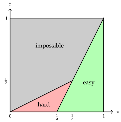
Figure 1: Computational versus statistical limits. For the submatrix detection problem, the size of the submatrix is $K=N^{\alpha}$ and the elevated mean is $\mu=N^{-\beta}$. For the community detection problem, the cluster size is $K=N^{\alpha}$, and the in-cluster and inter-cluster edge probability $p$ and $q$ are both on the order of $N^{-2\beta}$.

Specifically, consider the submatrix detection problem in the Gaussian case of Definition 1, where $P={\mathcal{N}}(\mu,1)$ and $Q={\mathcal{N}}(0,1)$. In other words, the goal is to test the null model, where the observation is an $N\times N$ Gaussian noise matrix, versus the planted model, where there exists a $K\times K$ submatrix of elevated mean $\mu$. Consider the high-dimensional setting of $K=N^{\alpha}$ and $\mu=N^{-\beta}$ with $N\to\infty$, where $\alpha,\beta>0$ parametrizes the cluster size and signal strength, respectively. Information-theoretically, it can be shown that there exist detection procedures achieving vanishing error probability if and only if $\beta<\beta^{*}\triangleq\max(\frac{\alpha}{2},2\alpha-1)$ [BI13]. In contrast, if only randomized polynomial-time algorithms are allowed, then reliable detection is impossible if $\beta>\beta^{\sharp}\triangleq\max(0,2\alpha-1)$; conversely if $\beta<\beta^{\sharp}$, there exists a near-linear time detection algorithm with vanishing error probability. Plotted in Fig. 1, the curve of $\beta^{*}$ and $\beta^{\sharp}$ corresponds to the statistical and computational limits of submatrix detection respectively, revealing the following striking phase transition: for large community ($\alpha\geq\frac{2}{3}$), optimal detection can be achieved by computationally efficient procedures; however, for small community ($\alpha<\frac{2}{3}$), computational constraint incurs a severe penalty on the statistical performance and the optimal computationally intensive procedure cannot be mimicked by any efficient algorithms.

For the Bernoulli case, it is shown to detect a planted dense subgraph, when the in-cluster and inter-cluster edge probability $p$ and $q$ are on the same order and parameterized as $N^{-2\beta}$ and the cluster size as $K=N^{\alpha}$, the easy-hard-impossible phase transition obeys the same diagram as in Fig. 1 [HWX15a].

Our intractability result is based on the common hardness assumption of the Planted Clique problem in the Erdős-Rényi graph when the clique size is of smaller order than square root the graph cardinality [AKS98], which has been widely used to establish various hardness results in theoretical computer science [HK11, AAK⁺07, KZ11, Kuč92, JP00, ABW10] as well as the hardness of detecting sparse principal components [BR13]. Recently, the average-case hardness of Planted Clique has been established under certain computation models [Ros10, FGR⁺13] and within the sum-of-squares relaxation hierarchy [MPW15, DM15b, BHK⁺16].

The rest of the section is organized as follows: Section 4.1 gives the precise definition of the Planted Clique problem, which forms the basis of reduction for both the submatrix detection and the community detection problem, with the latter requiring a slightly stronger assumption. Section 4.2 discusses how to approximately reduce the Planted Clique problem to the single community detection problem in polynomial-time in both Bernoulli and Gaussian settings. Finally, Section 4.3 presents the key techniques to bound the total variation between the reduced instance and to the target hypothesis.

4.1 Planted Clique problem

Let ${\mathcal{G}}(n,\gamma)$ denote the Erdős-Rényi graph model with $n$ vertices where each pair of vertices is connected independently with probability $\gamma$. Let ${\mathcal{G}}(n,k,\gamma)$ denote the planted clique model in which we add edges to $k$ vertices uniformly chosen from ${\mathcal{G}}(n,\gamma)$ to form a clique.

Definition 7.

The PC detection problem with parameters $(n,k,\gamma)$, denoted by ${\sf PC}(n,k,\gamma)$ henceforth, refers to the problem of testing the following hypotheses:

$$H^{\rm C}_{0}:\quad G\sim\mathcal{G}(n,\gamma),\quad\quad H^{\rm C}_{1}:\quad G\sim\mathcal{G}(n,k,\gamma).$$

The problem of finding the planted clique has been extensively studied for $\gamma=\frac{1}{2}$ and the state-of-the-art polynomial-time algorithms [AKS98, FK00, McS01, FR10, DGGP14, AV11, DM15a] only work for $k=\Omega(\sqrt{n})$. There is no known polynomial-time solver for the PC problem for $k=o(\sqrt{n})$ and any constant $\gamma>0$. It is conjectured [Jer92, HK11, JP00, AAK⁺07, FGR⁺13] that the PC problem cannot be solved in polynomial time for $k=o(\sqrt{n})$ with $\gamma=\frac{1}{2}$, which we refer to as the PC Hypothesis.

Hypothesis 1 (PC Hypothesis).

Fix some constant $0<\gamma\leq\frac{1}{2}$. For any sequence of randomized polynomial-time tests $\{\psi_{n,k_{n}}\}$ such that $\limsup_{n\to\infty}\frac{\log k_{n}}{\log n}<1/2$,

$$\liminf_{n\to\infty}\mathbb{P}_{H_{0}^{\rm C}}\{\psi_{n,k}(G)=1\}+\mathbb{P}_{H_{1}^{\rm C}}\{\psi_{n,k}(G)=0\}\geq 1.$$

The PC Hypothesis with $\gamma=\frac{1}{2}$ is similar to [MW15, Hypothesis 1] and [BR13, Hypothesis $\mathbf{B_{PC}}$]. Our computational lower bounds for submatrix detection require that the PC Hypothesis holds for $\gamma=\frac{1}{2}$ and for community detection we need to assume the PC Hypothesis any positive constant $\gamma$. An even stronger assumption that PC Hypothesis holds for $\gamma=2^{-\log^{0.99}n}$ has been used in [ABW10, Theorem 10.3] for public-key cryptography. Furthermore, [FGR⁺13, Corollary 5.8] shows that under a statistical query model, any statistical algorithm requires at least $n^{\Omega(\frac{\log n}{\log(1/\gamma)})}$ queries for detecting the planted bi-clique in an Erdős-Rényi random bipartite graph with edge probability $\gamma$.

4.2 Polynomial-time randomized reduction

We present a polynomial-time randomized reduction scheme for the problem of detecting a single community (Definition 1) in both Bernoulli and Gaussian cases. For ease of presentation, we use the Bernoulli case as the main example, and discuss the minor modifications needed for the Gaussian case. The recent work [BBH18] introduces a general reduction recipe for the single community detection problem under general $P,Q$ distributions, as well as various other detection problems with planted structures.

Let $\mathcal{G}(N,q)$ denote the Erdős-Rényi random graph with $N$ vertices, where each pair of vertices is connected independently with probability $q$. Let $\mathcal{G}(N,K,p,q)$ denote the planted dense subgraph model with $N$ vertices where: (1) each vertex is included in the random set $S$ independently with probability $\frac{K}{N}$; (2) for any two vertices, they are connected independently with probability $p$ if both of them are in $S$ and with probability $q$ otherwise, where $p>q$. The planted dense subgraph here has a random size with mean $K$, instead of a deterministic size $K$ as assumed in [ACV14, VAC⁺15].

Definition 8.

The planted dense subgraph detection problem with parameters $(N,K,p,q)$, henceforth denoted by ${\sf PDS}(N,K,p,q)$, refers to the problem of distinguishing hypotheses:

$$H_{0}:\quad G\sim\mathcal{G}(N,q)\triangleq\mathbb{P}_{0},\qquad H_{1}:\quad G\sim\mathcal{G}(N,K,p,q)\triangleq\mathbb{P}_{1}.$$

We aim to reduce the ${\sf PC}(n,k,\gamma)$ problem to the ${\sf PDS}(N,K,cq,q)$ problem. For simplicity, we focus on the case of $c=2$; the general case follows similarly with a change in some numerical constants that come up in the proof. We are given an adjacency matrix $A\in\{0,1\}^{n\times n}$, or equivalently, a graph $G,$ and with the help of additional randomness, will map it to an adjacency matrix ${\widetilde{A}}\in\{0,1\}^{N\times N},$ or equivalently, a graph ${\widetilde{G}}$ such that the hypothesis $H_{0}^{\rm C}$ (resp. $H_{1}^{\rm C}$) in Definition 7 is mapped to $H_{0}$ exactly (resp. $H_{1}$ approximately) in Definition 8. In other words, if $A$ is drawn from ${\mathcal{G}}(n,\gamma)$, then ${\widetilde{A}}$ is distributed according to $\mathbb{P}_{0}$; If $A$ is drawn from ${\mathcal{G}}(n,k,1,\gamma)$, then the distribution of ${\widetilde{A}}$ is close in total variation to $\mathbb{P}_{1}$.

Our reduction scheme works as follows. Each vertex in ${\widetilde{G}}$ is randomly assigned a parent vertex in $G,$ with the choice of parent being made independently for different vertices in ${\widetilde{G}},$ and uniformly over the set $[n]$ of vertices in $G.$ Let $V_{s}$ denote the set of vertices in ${\widetilde{G}}$ with parent $s\in[n]$ and let $\ell_{s}=|V_{s}|$. Then the set of children nodes $\{V_{s}:s\in[n]\}$ form a random partition of $[N]$. For any $1\leq s\leq t\leq n,$ the number of edges, $E(V_{s},V_{t})$, from vertices in $V_{s}$ to vertices in $V_{t}$ in ${\widetilde{G}}$ will be selected randomly with a conditional probability distribution specified below. Given $E(V_{s},V_{t}),$ the particular set of edges with cardinality $E(V_{s},V_{t})$ is chosen uniformly at random.

It remains to specify, for $1\leq s\leq t\leq n,$ the conditional distribution of $E(V_{s},V_{t})$ given $\ell_{s},\ell_{t},$ and $A_{s,t}.$ Ideally, conditioned on $\ell_{s}$ and $\ell_{t}$, we want to construct a Markov kernel from $A_{s,t}$ to $E(V_{s},V_{t})$ which maps ${\rm Bern}(1)$ to the desired edge distribution ${\rm Binom}(\ell_{s}\ell_{t},p)$, and ${\rm Bern}(1/2)$ to ${\rm Binom}(\ell_{s}\ell_{t},q)$, depending on whether both $s$ and $t$ are in the clique or not, respectively. Such a kernel, unfortunately, provably does not exist. Nevertheless, this objective can be accomplished approximately in terms of the total variation. For $s=t\in[n],$ let $E(V_{s},V_{t})\sim{\rm Binom}(\binom{\ell_{t}}{2},q).$ For $1\leq s<t\leq n$, denote $P_{\ell_{s}\ell_{t}}\triangleq{\rm Binom}(\ell_{s}\ell_{t},p)$ and $Q_{\ell_{s}\ell_{t}}\triangleq{\rm Binom}(\ell_{s}\ell_{t},q)$. Fix $0<\gamma\leq\frac{1}{2}$ and put $m_{0}\triangleq\lfloor\log_{2}(1/\gamma)\rfloor$. Define

$$P^{\prime}_{\ell_{s}\ell_{t}}(m)=\left\{\begin{array}[]{rl}P_{\ell_{s}\ell_{t}}(m)+a_{\ell_{s}\ell_{t}}&\text{for }m=0,\\ P_{\ell_{s}\ell_{t}}(m)&\text{for }1\leq m\leq m_{0},\\ \frac{1}{\gamma}Q_{\ell_{s}\ell_{t}}(m)&\text{for }m_{0}<m\leq\ell_{s}\ell_{t}.\end{array}\right.$$

where $a_{\ell_{s}\ell_{t}}=\sum_{m_{0}<m\leq\ell_{s}\ell_{t}}[P_{\ell_{s}\ell_{t}}(m)-\frac{1}{\gamma}Q_{\ell_{s}\ell_{t}}(m)]$. Let $Q^{\prime}_{\ell_{s}\ell_{t}}=\frac{1}{1-\gamma}(Q_{\ell_{s}\ell_{t}}-\gamma P^{\prime}_{\ell_{s}\ell_{t}})$. The idea behind our choice of $P^{\prime}_{\ell_{s}\ell_{t}}$ and $Q^{\prime}_{\ell_{s}\ell_{t}}$ is as follows. For a given $P^{\prime}_{\ell_{s}\ell_{t}}$, we choose $Q^{\prime}_{\ell_{s}\ell_{t}}$ to map ${\rm Bern}(\gamma)$ to ${\rm Binom}(\ell_{s}\ell_{t},q)$ exactly; however, for $Q^{\prime}$ to be a well-defined probability distribution, we need to ensure that $Q_{\ell_{s}\ell_{t}}(m)\geq\gamma P^{\prime}_{\ell_{s}\ell_{t}}(m)$, which fails when $m\leq m_{0}$. Thus, we set $P^{\prime}_{\ell_{s}\ell_{t}}(m)=Q_{\ell_{s}\ell_{t}}(m)/\gamma$ for $m>m_{0}$. The remaining probability mass $a_{\ell_{s}\ell_{t}}$ is added to $P_{\ell_{s}\ell_{t}}(0)$ so that $P^{\prime}_{\ell_{s}\ell_{t}}$ is a well-defined probability distribution.

It is straightforward to verify that $Q^{\prime}_{\ell_{s}\ell_{t}}$ and $P^{\prime}_{\ell_{s}\ell_{t}}$ are well-defined probability distributions, and

$$d_{\rm TV}(P^{\prime}_{\ell_{s}\ell_{t}},P_{\ell_{s}\ell_{t}})\leq 4(8q\ell^{2})^{(m_{0}+1)}.$$ (36)

as long as $\ell_{s},\ell_{t}\leq 2\ell$ and $16q\ell^{2}\leq 1$, where $\ell=N/n$. Then, for $1\leq s<t\leq n,$ the conditional distribution of $E(V_{s},V_{t})$ given $\ell_{s},\ell_{t},$ and $A_{s,t}$ is given by

$$E(V_{s},V_{t})\sim\left\{\begin{array}[]{rl}P^{\prime}_{\ell_{s}\ell_{t}}&\text{if }A_{st}=1,\ell_{s},\ell_{t}\leq 2\ell\\ Q^{\prime}_{\ell_{s}\ell_{t}}&\text{if }A_{st}=0,\ell_{s},\ell_{t}\leq 2\ell\\ Q_{\ell_{s}\ell_{t}}&\text{if }\max\{\ell_{s},\ell_{t}\}>2\ell.\end{array}\right.$$ (40)

Next we show that the randomized reduction defined above maps ${\mathcal{G}}(n,\gamma)$ into ${\mathcal{G}}(N,q)$ under the null hypothesis and ${\mathcal{G}}(n,k,\gamma)$ approximately into ${\mathcal{G}}(N,K,p,q)$ under the alternative hypothesis, respectively. By construction, $(1-\gamma)Q^{\prime}_{\ell_{s}\ell_{t}}+\gamma P^{\prime}_{\ell_{s}\ell_{t}}=Q_{\ell_{s}\ell_{t}}={\rm Binom}(\ell_{s}\ell_{t},q)$ and therefore the null distribution of the PC problem is exactly matched to that of the PDS problem, i.e., $P_{{\widetilde{G}}|H_{0}^{C}}=\mathbb{P}_{0}$. The core of the proof lies in establishing that the alternative distributions are approximately matched. The key observation is that by (36), $P^{\prime}_{\ell_{s}\ell_{t}}$ is close to $P_{\ell_{s}\ell_{t}}={\rm Binom}(\ell_{s}\ell_{t},p)$ and thus for nodes with distinct parents $s\neq t$ in the planted clique, the number of edges $E(V_{s},V_{t})$ is approximately distributed as the desired ${\rm Binom}(\ell_{s}\ell_{t},p)$; for nodes with the same parent $s$ in the planted clique, even though $E(V_{s},V_{s})$ is distributed as ${\rm Binom}(\binom{\ell_{s}}{2},q)$ which is not sufficiently close to the desired ${\rm Binom}(\binom{\ell_{s}}{2},p)$, after averaging over the random partition $\{V_{s}\}$, the total variation distance becomes negligible. More formally, we have the following proposition; the proof is postponed to the next subsection.

Proposition 1.

Let $\ell,n\in{\mathbb{N}}$, $k\in[n]$ and $\gamma\in(0,\frac{1}{2}]$. Let $N=\ell n$, $K=k\ell$, $p=2q$ and $m_{0}=\lfloor\log_{2}(1/\gamma)\rfloor$. Assume that $16q\ell^{2}\leq 1$ and $k\geq 6e\ell$. If $G\sim\mathcal{G}(n,\gamma)$, then ${\widetilde{G}}\sim{\mathcal{G}}(N,q)$, i.e., $P_{{\widetilde{G}}|H_{0}^{C}}=\mathbb{P}_{0}$. If $G\sim{\mathcal{G}}(n,k,1,\gamma)$, then

$$d_{\rm TV}\left(P_{{\widetilde{G}}|H_{1}^{C}},\mathbb{P}_{1}\right)$$

$$\leq e^{-\frac{K}{12}}+1.5ke^{-\frac{\ell}{18}}+2k^{2}(8q\ell^{2})^{m_{0}+1}+0.5\sqrt{e^{72e^{2}q\ell^{2}}-1}+\sqrt{0.5k}e^{-\frac{\ell}{36}}.$$ (41)

Reduction scheme in the Gaussian case

The same reduction scheme can be tweaked slightly to work for the Gaussian case, which, in fact, only needs the PC hypothesis for $\gamma=\frac{1}{2}$. In this case, we aim to map an adjacency matrix $A\in\{0,1\}^{n\times n}$ to a symmetric data matrix ${\widetilde{A}}\in{\mathbb{R}}^{N\times N}$ with zero diagonal, or equivalently, a weighted complete graph ${\widetilde{G}}$.

For any $1\leq s\leq t\leq n,$ we let $E(V_{s},V_{t})$ denote the average weights of edges between $V_{s}$ and $V_{t}$ in ${\widetilde{G}}$. Similar to the Bernoulli model, we will first generate $E(V_{s},V_{t})$ randomly with a properly chosen conditional probability distribution. Since $E(V_{s},V_{t})$ is a sufficient statistic for the set of Gaussian edge weights, the specific weight assignment can be generated from the average weight using the same kernel for both the null and the alternative.

To see how this works, consider a general setup where $X_{1},\ldots,X_{n}{\stackrel{{\scriptstyle\text{i.i.d.}}}{{\sim}}}{\mathcal{N}}(\mu,1)$. Let $\bar{X}=(1/n)\sum_{i=1}^{n}X_{i}$. Then we can simulate $X_{1},\ldots,X_{n}$ based on the sufficient statistic $\bar{X}$ as follows. Let $[v_{0},v_{1},\ldots,v_{n-1}]$ be an orthonormal basis for ${\mathbb{R}}^{n}$, with $v_{0}=\frac{1}{\sqrt{n}}\mathbf{1}$ and $\mathbf{1}=(1,\ldots,1)^{\top}$. Generate $Z_{1},\ldots,Z_{n-1}{\stackrel{{\scriptstyle\text{i.i.d.}}}{{\sim}}}{\mathcal{N}}(0,1)$. Then $\bar{X}\mathbf{1}+\sum_{i=1}^{n-1}Z_{i}v_{i}\sim{\mathcal{N}}(\mu\mathbf{1},I_{n})$. Using this general procedure, we can generate the weights ${\widetilde{A}}_{V_{s},V_{t}}$ based on $E(V_{s},V_{t})$.

It remains to specify, for $1\leq s\leq t\leq n,$ the conditional distribution of $E(V_{s},V_{t})$ given $\ell_{s},\ell_{t},$ and $A_{s,t}.$ Similar to the Bernoulli case, conditioned on $\ell_{s}$ and $\ell_{t}$, ideally we would want to find a Markov kernel from $A_{s,t}$ to $E(V_{s},V_{t})$ which maps ${\rm Bern}(1)$ to the desired distribution ${\mathcal{N}}(\mu,1/\ell_{s}\ell_{t})$, and ${\rm Bern}(1/2)$ to ${\mathcal{N}}(0,1/\ell_{s}\ell_{t})$, depending on whether both $s$ and $t$ are in the clique or not, respectively. This objective can be accomplished approximately in terms of the total variation. For $s=t\in[n],$ let $E(V_{s},V_{t})\sim{\mathcal{N}}(0,1/\ell_{s}\ell_{t}).$ For $1\leq s<t\leq n$, denote $P_{\ell_{s}\ell_{t}}\triangleq{\mathcal{N}}(\mu,1/\ell_{s}\ell_{t})$ and $Q_{\ell_{s}\ell_{t}}\triangleq{\mathcal{N}}(0,1/\ell_{s}\ell_{t})$, with density function $p_{\ell_{s}\ell_{t}}(x)$ and $q_{\ell_{s}\ell_{t}}(x)$, respectively.

Fix $\gamma=\frac{1}{2}$. Note that

$$\frac{q_{\ell_{s}\ell_{t}}(x)}{p_{\ell_{s}\ell_{t}}(x)}=\exp\left[\ell_{s}\ell_{t}\mu(\mu/2-x)\right]\geq\gamma$$

if and only if $x\leq x_{0}\triangleq\frac{\mu}{2}+\frac{1}{\mu\ell_{s}\ell_{t}}\log\frac{1}{\gamma}$. Therefore, we define $P^{\prime}_{\ell_{s}\ell_{t}}$ and $Q^{\prime}_{\ell_{s}\ell_{t}}$ with the following density: $q^{\prime}_{\ell_{s}\ell_{t}}=\frac{1}{1-\gamma}(q_{\ell_{s}\ell_{t}}-\gamma p^{\prime}_{\ell_{s}\ell_{t}})$ and

$$p^{\prime}_{\ell_{s}\ell_{t}}(x)=\left\{\begin{array}[]{rl}p_{\ell_{s}\ell_{t}}(x)+f_{\ell s\ell_{t}}(2\mu-x)&\text{for }x<2\mu-x_{0},\\ p_{\ell_{s}\ell_{t}}(x)&\text{for }x\leq x_{0},\\ \frac{1}{\gamma}q_{\ell_{s}\ell_{t}}(x)&\text{for }x>x_{0}.\end{array}\right.$$

where $f_{\ell s\ell_{t}}(x)=p_{\ell_{s}\ell_{t}}(x)-\frac{1}{\gamma}q_{\ell_{s}\ell_{t}}(x)$. Let

$$a_{\ell_{s}\ell_{t}}=\int_{x_{0}}^{\infty}f_{\ell s\ell_{t}}(x)dx\leq\bar{\Phi}\left(-\frac{\mu}{2}\sqrt{\ell_{s}\ell_{t}}+\frac{1}{\mu\sqrt{\ell_{s}\ell_{t}}}\log\frac{1}{\gamma}\right).$$

Similar to the Bernoulli case, it is straightforward to verify that $Q^{\prime}_{\ell_{s}\ell_{t}}$ and $P^{\prime}_{\ell_{s}\ell_{t}}$ are well-defined probability distributions, and

$$d_{\rm TV}(P^{\prime}_{\ell_{s}\ell_{t}},P_{\ell_{s}\ell_{t}})=a_{\ell_{s}\ell_{t}}\leq\bar{\Phi}\left(\frac{1}{2\mu\sqrt{\ell_{s}\ell_{t}}}\log\frac{1}{\gamma}\right)\leq\exp\left(-\frac{1}{32\mu^{2}\ell^{2}}\log^{2}\frac{1}{\gamma}\right).$$ (42)

as long as $\ell_{s},\ell_{t}\leq 2\ell$ and $4\mu^{2}\ell^{2}\leq\log(1/\gamma)$, where $\ell=N/n$. Following the same argument as Bernoulli case, we can obtain a counterpart to Proposition 1.

Proposition 2.

Let $\ell,n\in{\mathbb{N}}$, $k\in[n]$ and $\gamma=1/2$. Let $N=\ell n$ and $K=k\ell$ Assume that $16\mu^{2}\ell\leq 1$ and $k\geq 6e\ell$. Let $\mathbb{P}_{0}$ and $\mathbb{P}_{1}$ denote the desired null and alternative distributions of the submatrix detection problem $(N,K,\mu)$. If $G\sim\mathcal{G}(n,\gamma)$, then $P_{{\widetilde{G}}|H_{0}^{C}}=\mathbb{P}_{0}$. If $G\sim{\mathcal{G}}(n,k,1,\gamma)$, then

$$d_{\rm TV}\left(P_{{\widetilde{G}}|H_{1}^{C}},\mathbb{P}_{1}\right)$$

$$\leq e^{-\frac{K}{12}}+1.5ke^{-\frac{\ell}{18}}+\frac{k^{2}}{2}\exp\left(-\frac{\log^{2}2}{32\mu^{2}\ell^{2}}\right)+0.5\sqrt{e^{72e^{2}\mu^{2}\ell^{2}}-1}+\sqrt{0.5k}e^{-\frac{\ell}{36}}.$$ (43)

Let us close this section with two remarks. First, to investigate the computational aspect of inference in the Gaussian model, since the computational complexity is not well-defined for tests dealing with samples drawn from non-discrete distributions, which cannot be represented by finitely many bits almost surely. To overcome this hurdle, we consider a sequence of discretized Gaussian models that is asymptotically equivalent to the original model in the sense of Le Cam [LC86] and hence preserves the statistical difficulty of the problem. In other words, the continuous model and its appropriately discretized counterpart are statistically indistinguishable and, more importantly, the computational complexity of tests on the latter are well-defined. More precisely, for the submatrix detection model, provided that each entry of the $n\times n$ matrix $A$ is quantized by $\Theta(\log n)$ bits, the discretized model is asymptotically equivalent to the previous model (cf. [MW15, Section 3 and Theorem 1] for a precise bound on the Le Cam distance). With a slight modification, the above reduction scheme can be made to the discretized model (cf. [MW15, Section 4.2]).

Second, we comment on the distinctions between the reduction scheme here and the prior work that relies on planted clique as the hardness assumption. Most previous work [HK11, AAK⁺07, AAM⁺11, ABW10] in the theoretical computer science literature uses the reduction from the PC problem to generate computationally hard instances of other problems and establish worst-case hardness results; the underlying distributions of the instances could be arbitrary. The idea of proving hardness of a hypothesis testing problem by means of approximate reduction from the planted clique problem such that the reduced instance is close to the target hypothesis in total variation originates from the seminal work by [BR13] and the subsequent paper by [MW15]. The main distinction between these work and the results presented in this article based on the techniques in [HWX15a] is that [BR13] studied a composite-versus-composite testing problem and [MW15] studied a simple-versus-composite testing problem, both in the minimax sense, as opposed to the simple-versus-simple hypothesis considered here and in [HWX15a], which constitutes a stronger hardness result. For composite hypothesis, a reduction scheme works as long as the distribution of the reduced instance is close to some mixture distribution under the hypothesis. This freedom is absent in constructing reduction for simple hypothesis, which renders the reduction scheme as well as the corresponding calculation of total variation considerably more difficult. In contrast, for simple-versus-simple hypothesis, the underlying distributions of the problem instances generated from the reduction must be close to the desired distributions in total variation under both the null and alternative hypotheses.

4.3 Bounding the total variation distance

Below we prove Proposition 1 and obtain the desired computational limits given by Fig. 1. We only consider the Bernoulli case as the derivations for Gaussian case are analogous. The main technical challenge is bounding the total variation distance in (41).

Proof of Proposition 1.

Let $[i,j]$ denote the unordered pair of $i$ and $j$. For any set $I\subset[N]$, let ${\mathcal{E}}(I)$ denote the set of unordered pairs of distinct elements in $I$, i.e., ${\mathcal{E}}(I)=\{[i,j]:i,j\in S,i\neq j\}$, and let ${\mathcal{E}}(I)^{c}={\mathcal{E}}([N])\setminus{\mathcal{E}}(I)$. For $s,t\in[n]$ with $s\neq t$, let ${\widetilde{G}}_{V_{s}V_{t}}$ denote the bipartite graph where the set of left (right) vertices is $V_{s}$ (resp. $V_{t}$) and the set of edges is the set of edges in ${\widetilde{G}}$ from vertices in $V_{s}$ to vertices in $V_{t}$. For $s\in[n]$, let ${\widetilde{G}}_{V_{s}V_{s}}$ denote the subgraph of ${\widetilde{G}}$ induced by $V_{s}$. Let ${\widetilde{P}}_{V_{s}V_{t}}$ denote the edge distribution of ${\widetilde{G}}_{V_{s}V_{t}}$ for $s,t\in[n]$.

It is straightforward to verify that the null distributions are exactly matched by the reduction scheme. Henceforth, we consider the alternative hypothesis, under which $G$ is drawn from the planted clique model $\mathcal{G}(n,k,\gamma)$. Let $C\subset[n]$ denote the planted clique. Define $S=\cup_{t\in C}V_{t}$ and recall $K=k\ell$. Then $|S|\sim{\rm Binom}(N,K/N)$ and conditional on $|S|$, $S$ is uniformly distributed over all possible subsets of size $|S|$ in $[N]$. By the symmetry of the vertices of $G$, the distribution of ${\widetilde{A}}$ conditional on $C$ does not depend on $C$. Hence, without loss of generality, we shall assume that $C=[k]$ henceforth. The distribution of $\widetilde{A}$ can be written as a mixture distribution indexed by the random set $S$ as

$$\widetilde{A}\sim\widetilde{\mathbb{P}}_{1}\triangleq\mathbb{E}_{S}\left[{\widetilde{P}}_{SS}\times\prod_{[i,j]\in{\mathcal{E}}(S)^{c}}{\rm Bern}(q)\right].$$

By the definition of $\mathbb{P}_{1}$,

$$d_{\rm TV}(\widetilde{\mathbb{P}}_{1},\mathbb{P}_{1})$$

$$=d_{\rm TV}\left(\mathbb{E}_{S}\left[{\widetilde{P}}_{SS}\times\prod_{[i,j]\in{\mathcal{E}}(S)^{c}}{\rm Bern}(q)\right],\mathbb{E}_{S}\left[\prod_{[i,j]\in{\mathcal{E}}(S)}{\rm Bern}(p)\prod_{[i,j]\in{\mathcal{E}}(S)^{c}}{\rm Bern}(q)\right]\right)$$

$$\leq\mathbb{E}_{S}\left[d_{\rm TV}\left({\widetilde{P}}_{SS}\times\prod_{[i,j]\in{\mathcal{E}}(S)^{c}}{\rm Bern}(q),\prod_{[i,j]\in{\mathcal{E}}(S)}{\rm Bern}(p)\prod_{[i,j]\in{\mathcal{E}}(S)^{c}}{\rm Bern}(q)\right)\right]$$

$$=\mathbb{E}_{S}\left[d_{\rm TV}\left({\widetilde{P}}_{SS},\prod_{[i,j]\in{\mathcal{E}}(S)}{\rm Bern}(p)\right)\right]$$

$$\leq\mathbb{E}_{S}\left[d_{\rm TV}\left({\widetilde{P}}_{SS},\prod_{[i,j]\in{\mathcal{E}}(S)}{\rm Bern}(p)\right){\mathbf{1}_{\left\{{|S|\leq 1.5K}\right\}}}\right]+\exp(-K/12),$$ (44)

where the first inequality follows from the convexity of $(P,Q)\mapsto d_{\rm TV}(P,Q)$, and the last inequality follows from applying the Chernoff bound to $|S|$. Fix an $S\subset[N]$ such that $|S|\leq 1.5K$. Define $P_{V_{t}V_{t}}=\prod_{[i,j]\in{\mathcal{E}}(V_{t})}{\rm Bern}(q)$ for $t\in[k]$ and $P_{V_{s}V_{t}}=\prod_{(i,j)\in V_{s}\times V_{t}}{\rm Bern}(p)$ for $1\leq s<t\leq k$. By the triangle inequality,

$$d_{\rm TV}\left({\widetilde{P}}_{SS},\prod_{[i,j]\in{\mathcal{E}}(S)}{\rm Bern}(p)\right)$$

$$\leq ~{}d_{\rm TV}\left({\widetilde{P}}_{SS},\mathbb{E}_{V_{1}^{k}}\left[\prod_{1\leq s\leq t\leq k}P_{V_{s}V_{t}}\biggm{|}S\right]\right)$$ (45)

$$~{}+d_{\rm TV}\left(\mathbb{E}_{V_{1}^{k}}\left[\prod_{1\leq s\leq t\leq k}P_{V_{s}V_{t}}\biggm{|}S\right],\prod_{[i,j]\in{\mathcal{E}}(S)}{\rm Bern}(p)\right).$$ (46)

To bound the term in (45), first note that conditioned on the set $S$, $\{V_{1}^{k}\}$ can be generated as follows: Throw balls indexed by $S$ into bins indexed by $[k]$ independently and uniformly at random; let $V_{t}$ is the set of balls in the $t^{\rm th}$ bin. Define the event $E=\{V_{1}^{k}:|V_{t}|\leq 2\ell,t\in[k]\}$. Since $|V_{t}|\sim{\rm Binom}(|S|,1/k)$ is stochastically dominated by ${\rm Binom}(1.5K,1/k)$ for each fixed $1\leq t\leq k$, it follows from the Chernoff bound and the union bound that $\mathbb{P}\{E^{c}\}\leq k\exp(-\ell/18)$.

$$d_{\rm TV}\left({\widetilde{P}}_{SS},\mathbb{E}_{V_{1}^{k}}\left[\prod_{1\leq s\leq t\leq k}P_{V_{s}V_{t}}\biggm{|}S\right]\right)$$

$$\overset{(a)}{=}d_{\rm TV}\left(\mathbb{E}_{V_{1}^{k}}\left[\prod_{1\leq s\leq t\leq k}\widetilde{P}_{V_{s}V_{t}}\biggm{|}S\right],\mathbb{E}_{V_{1}^{k}}\left[\prod_{1\leq s\leq t\leq k}P_{V_{s}V_{t}}\biggm{|}S\right]\right)$$

$$\leq\mathbb{E}_{V_{1}^{k}}\left[d_{\rm TV}\left(\prod_{1\leq s\leq t\leq k}\widetilde{P}_{V_{s}V_{t}},\prod_{1\leq s\leq t\leq k}P_{V_{s}V_{t}}\right)\biggm{|}S\right]$$

$$\leq\mathbb{E}_{V_{1}^{k}}\left[d_{\rm TV}\left(\prod_{1\leq s\leq t\leq k}\widetilde{P}_{V_{s}V_{t}},\prod_{1\leq s\leq t\leq k}P_{V_{s}V_{t}}\right){\mathbf{1}_{\left\{{V_{1}^{k}\in E}\right\}}}\biggm{|}S\right]+k\exp(-\ell/18),$$

where $(a)$ holds because conditional on $V_{1}^{k}$, $\{{\widetilde{A}}_{V_{s}V_{t}}:s,t\in[k]\}$ are independent. Recall that $\ell_{t}=|V_{t}|$. For any fixed $V_{1}^{k}\in E$, we have

$$d_{\rm TV}\left(\prod_{1\leq s\leq t\leq k}\widetilde{P}_{V_{s}V_{t}},\prod_{1\leq s\leq t\leq k}P_{V_{s}V_{t}}\right)$$

$$\overset{(a)}{=}d_{\rm TV}\left(\prod_{1\leq s<t\leq k}\widetilde{P}_{V_{s}V_{t}},\prod_{1\leq s<t\leq k}P_{V_{s}V_{t}}\right)$$

$$\overset{(b)}{=}d_{\rm TV}\left(\prod_{1\leq s<t\leq k}P^{\prime}_{\ell_{s}\ell_{t}},\prod_{1\leq s<t\leq k}P_{\ell_{s}\ell_{t}}\right)$$

$$\leq d_{\rm TV}\left(\prod_{1\leq s<t\leq k}P^{\prime}_{\ell_{s}\ell_{t}},\prod_{1\leq s<t\leq k}P_{\ell_{s}\ell_{t}}\right)$$

$$\leq\sum_{1\leq s<t\leq k}d_{\rm TV}\left(P^{\prime}_{\ell_{s}\ell_{t}},P_{\ell_{s}\ell_{t}}\right)\overset{(c)}{\leq}2k^{2}(8q\ell^{2})^{(m_{0}+1)},$$

where $(a)$ follows since ${\widetilde{P}}_{V_{t}V_{t}}=P_{V_{t}V_{t}}$ for all $t\in[k]$; $(b)$ is because the number of edges $E(V_{s},V_{t})$ is a sufficient statistic for testing ${\widetilde{P}}_{V_{s}V_{t}}$ versus $P_{V_{s}V_{t}}$ on the submatrix $A_{V_{s}V_{t}}$ of the adjacency matrix; $(c)$ follows from the total variation bound (36). Therefore,

$$d_{\rm TV}\left({\widetilde{P}}_{SS},\mathbb{E}_{V_{1}^{k}}\left[\prod_{1\leq s\leq t\leq k}P_{V_{s}V_{t}}\biggm{|}S\right]\right)\leq 2k^{2}(8q\ell^{2})^{(m_{0}+1)}+k\exp(-\ell/18).$$ (47)

To bound the term in (46), applying [HWX15a][Lemma 9], which is a conditional version of the second moment method, yields

$$d_{\rm TV}\left(\mathbb{E}_{V_{1}^{k}}\left[\prod_{1\leq s\leq t\leq k}P_{V_{s}V_{t}}\biggm{|}S\right],\prod_{[i,j]\in{\mathcal{E}}(S)}{\rm Bern}(p)\right)$$

$$\leq\frac{1}{2}\mathbb{P}\left\{E^{c}\right\}+\frac{1}{2}\sqrt{\mathbb{E}_{V_{1}^{k};{\widetilde{V}}_{1}^{k}}\left[g(V_{1}^{k},{\widetilde{V}}_{1}^{k}){\mathbf{1}_{\left\{{V_{1}^{k}\in E}\right\}}}{\mathbf{1}_{\left\{{{\widetilde{V}}_{1}^{k}\in E}\right\}}}\biggm{|}S\right]-1+2\mathbb{P}\left\{E^{c}\right\}},$$ (48)

where

$$g(V_{1}^{k},{\widetilde{V}}_{1}^{k}) =\int\frac{\prod_{1\leq s\leq t\leq k}P_{V_{s}V_{t}}\prod_{1\leq s\leq t\leq k}P_{{\widetilde{V}}_{s}{\widetilde{V}}_{t}}}{\prod_{[i,j]\in{\mathcal{E}}(S)}{\rm Bern}(p)}$$

$$=\prod_{s,t=1}^{k}\left(\frac{q^{2}}{p}+\frac{(1-q)^{2}}{1-p}\right)^{\binom{|V_{s}\cap{\widetilde{V}}_{t}|}{2}}=\prod_{s,t=1}^{k}\left(\frac{1-\frac{3}{2}q}{1-2q}\right)^{\binom{|V_{s}\cap{\widetilde{V}}_{t}|}{2}}.$$

Let $X\sim\text{Bin}(1.5K,\frac{1}{k^{2}})$ and $Y\sim\text{Bin}(3\ell,e/k)$. It follows that

$$\mathbb{E}_{V_{1}^{k};{\widetilde{V}}_{1}^{k}}\left[\prod_{s,t=1}^{k}\left(\frac{1-\frac{3}{2}q}{1-2q}\right)^{\binom{|V_{s}\cap{\widetilde{V}}_{t}|}{2}}\prod_{s,t=1}^{k}{\mathbf{1}_{\left\{{|V_{s}|\leq 2\ell,|{\widetilde{V}}_{t}|\leq 2\ell}\right\}}}\biggm{|}S\right]$$

$$\overset{(a)}{\leq}\mathbb{E}_{V_{1}^{k};{\widetilde{V}}_{1}^{k}}\left[\prod_{s,t=1}^{k}e^{q\binom{|V_{s}\cap{\widetilde{V}}_{t}|\wedge 2\ell}{2}}\biggm{|}S\right]$$

$$\stackrel{{\scriptstyle(b)}}{{\leq}}~{}\prod_{s,t=1}^{k}\mathbb{E}\left[e^{q\binom{|V_{s}\cap{\widetilde{V}}_{t}|\wedge 2\ell}{2}}\biggm{|}S\right]$$

$$\overset{(c)}{\leq}\left(\mathbb{E}\left[e^{q\binom{X\wedge 2\ell}{2}}\right]\right)^{k^{2}}\overset{(d)}{\leq}\mathbb{E}\left[e^{q\binom{Y}{2}}\right]^{k^{2}}\overset{(e)}{\leq}\exp(72e^{2}q\ell^{2}),$$ (49)

where $(a)$ follows from $1+x\leq e^{x}$ for all $x\geq 0$ and $q<1/4$; $(b)$ follows from the negative association property of $\{|V_{s}\cap{\widetilde{V}}_{t}|:s,t\in[k]\}$ proved in [HWX15a][Lemma 10] in view of the monotonicity of $x\mapsto e^{q\binom{x\wedge 2\ell}{2}}$ on ${\mathbb{R}}_{+}$; $(c)$ follows because $|V_{s}\cap{\widetilde{V}}_{t}|$ is stochastically dominated by ${\rm Binom}(1.5K,1/k^{2})$ for all $(s,t)\in[k]^{2}$; $(d)$ follows from [HWX15a][Lemma 11]); $(e)$ follows from [HWX15a][Lemma 12] with $\lambda=q/2$ and $q\ell\leq 1/8$. Therefore, by (48)

$$d_{\rm TV}\left({\widetilde{P}}_{SS},\prod_{[i,j]\in{\mathcal{E}}(S)}{\rm Bern}(p)\right) \leq 0.5ke^{-\frac{\ell}{18}}+0.5\sqrt{e^{72e^{2}q\ell^{2}}-1+2ke^{-\frac{\ell}{18}}}$$

$$\leq 0.5ke^{-\frac{\ell}{18}}+0.5\sqrt{e^{72e^{2}q\ell^{2}}-1}+\sqrt{0.5k}e^{-\frac{\ell}{36}}.$$ (50)

Proposition 1 follows by combining (44), (45), (46), (47) and (50). ∎

The following theorem establishes the computational hardness of the ${\sf PDS}$ problem in the interior of the red region in Fig. 1.

Theorem 3.

Assume PC Hypothesis (Hypothesis 1) holds for all $0<\gamma\leq 1/2$. Let $\alpha>0$ and $0<\beta<1$ be such that

$$\max\{0,2\alpha-1\}\triangleq\beta^{\sharp}<\beta<\frac{\alpha}{2}.$$ (51)

Then there exists a sequence $\{(N_{\ell},K_{\ell},q_{\ell})\}_{\ell\in{\mathbb{N}}}$ satisfying

$$\lim_{\ell\to\infty}\frac{\log(1/q_{\ell})}{\log N_{\ell}}=2\beta,\quad\lim_{\ell\to\infty}\frac{\log K_{\ell}}{\log N_{\ell}}=\alpha$$

such that for any sequence of randomized polynomial-time tests $\phi_{\ell}:\{0,1\}^{\binom{N_{\ell}}{2}}\to\{0,1\}$ for the ${\sf PDS}(N_{\ell},K_{\ell},2q_{\ell},q_{\ell})$ problem, the Type-I+II error probability is lower bounded by

$$\liminf_{\ell\to\infty}\mathbb{P}_{0}\{\phi_{\ell}(G^{\prime})=1\}+\mathbb{P}_{1}\{\phi_{\ell}(G^{\prime})=0\}\geq 1,$$

where $G^{\prime}\sim{\mathcal{G}}(N,q)$ under $H_{0}$ and $G^{\prime}\sim{\mathcal{G}}(N,K,p,q)$ under $H_{1}$.

Proof.

Let $m_{0}=\lfloor\log_{2}(1/\gamma)\rfloor$. By (51), there exist $0<\gamma\leq 1/2$ and thus $m_{0}$ such that

$$2\beta<\alpha<\frac{1}{2}+\frac{m_{0}\beta+2}{2m_{0}\beta+1}\beta-\frac{1}{m_{0}\beta}.$$ (52)

Fix $\beta>0$ and $0<\alpha<1$ that satisfy (52). Let $\delta=1/(m_{0}\beta)$. Then it is straightforward to verify that $\frac{2+m_{0}\delta}{2+\delta}\beta\geq\frac{1}{2}-\delta+\frac{1+2\delta}{2+\delta}\beta$. It follows from the assumption (52) that

$$2\beta<\alpha<\min\left\{\frac{2+m_{0}\delta}{2+\delta}\beta,\;\frac{1}{2}-\delta+\frac{1+2\delta}{2+\delta}\beta\right\}.$$ (53)

Let $\ell\in{\mathbb{N}}$ and $q_{\ell}=\ell^{-(2+\delta)}$. Define

$$n_{\ell}=\lfloor\ell^{\frac{2+\delta}{2\beta}-1}\rfloor,\;k_{\ell}=\lfloor\ell^{\frac{(2+\delta)\alpha}{2\beta}-1}\rfloor,\;N_{\ell}=n_{\ell}\ell,\;K_{\ell}=k_{\ell}\ell.$$ (54)

Then

$$\lim_{\ell\to\infty}\frac{\log\frac{1}{q_{\ell}}}{\log N_{\ell}} =\frac{(2+\delta)}{(2+\delta)/(2\beta)-1+1}=2\beta,$$

$$\lim_{\ell\to\infty}\frac{\log K_{\ell}}{\log N_{\ell}} =\frac{(2+\delta)\alpha/(2\beta)-1+1}{(2+\delta)/(2\beta)-1+1}=\alpha.$$ (55)

Suppose that for the sake of contradiction there exists a small $\epsilon>0$ and a sequence of randomized polynomial-time tests $\{\phi_{\ell}\}$ for ${\sf PDS}(N_{\ell},K_{\ell},2q_{\ell},q_{\ell})$, such that

$$\mathbb{P}_{0}\{\phi_{N_{\ell},K_{\ell}}(G^{\prime})=1\}+\mathbb{P}_{1}\{\phi_{N_{\ell},K_{\ell}}(G^{\prime})=0\}\leq 1-\epsilon$$

holds for arbitrarily large $\ell$, where $G^{\prime}$ is the graph in the ${\sf PDS}(N_{\ell},K_{\ell},2q_{\ell},q_{\ell})$. Since $\alpha>2\beta$, we have $k_{\ell}\geq\ell^{1+\delta}$. Therefore, $16q_{\ell}\ell^{2}\leq 1$ and $k_{\ell}\geq 6e\ell$ for all sufficiently large $\ell$. Applying Proposition 1, we conclude that $G\mapsto\phi({\widetilde{G}})$ is a randomized polynomial-time test for ${\sf PC}(n_{\ell},k_{\ell},\gamma)$ whose Type-I+II error probability satisfies

$$\mathbb{P}_{H_{0}^{\rm C}}\{\phi_{\ell}({\widetilde{G}})=1\}+\mathbb{P}_{H_{1}^{\rm C}}\{\phi_{\ell}({\widetilde{G}})=0\}\leq 1-\epsilon+\xi,$$ (56)

where $\xi$ is given by the right-hand side of (41). By the definition of $q_{\ell}$, we have $q_{\ell}\ell^{2}=\ell^{-\delta}$ and thus

$$k_{\ell}^{2}(q_{\ell}\ell^{2})^{m_{0}+1}\leq\ell^{(2+\delta)\alpha/\beta-2-(m_{0}+1)\delta}\leq\ell^{-\delta},$$

where the last inequality follows from (53). Therefore $\xi\to 0$ as $\ell\to\infty$. Moreover, by the definition in (54),

$$\lim_{\ell\to\infty}\frac{\log k_{\ell}}{\log n_{\ell}}=\frac{(2+\delta)\alpha/(2\beta)-1}{(2+\delta)/(2\beta)-1}\leq\frac{1}{2}-\delta,$$

where the above inequality follows from (53). Therefore, (56) contradicts the assumption that PC Hypothesis (Hypothesis 1) holds for $\gamma$. ∎

5 Discussions and open problems

Recent years have witnessed a great deal of progress on understanding the information-theoretical and computational limits of various statistical problems with planted structures. As outlined in this survey, various techniques are in place to identify the information-theoretic limits. In some cases, polynomial-time procedures are shown to achieve the information-theoretic limits. However, in many other cases, it is believed that there exists a wide gap between the information-theoretic limits and the computational limits. For the planted clique problem, a recent exciting line of research has identified the performance limits of sum-of-squares hierarchy [MPW15, DM15b, HKP15, RS15, BHK⁺16]. Under PC Hypothesis, complexity-theoretic computational lower bounds have been derived for sparse PCA [BR13], submatrix location [MW15], single community detection [HWX15a], and various other detection problems with planted structures [BBH18]. Despite these encouraging results, a variety of interesting questions remain open. Below we list a few representative problems. Closing the observed computational gap, or equally importantly, disproving the possibility thereof on rigorous complexity-theoretic grounds, is an exciting new topic at the intersection of high-dimensional statistics, information theory, and computer science.

Computational lower bounds for recovering the planted dense subgraph

Closely related to the PDS detection problem is the recovery problem, where given a graph generated from ${\mathcal{G}}(N,K,p,q)$, the task is to recover the planted dense subgraph. Consider the asymptotic regime depicted in Fig. 1. It has been shown in [CX14, Ame13] that exact recovery is information-theoretically possible if and only if $\beta<\alpha/2$ and can be achieved in polynomial-time if $\beta<\alpha-\frac{1}{2}$. Our computational lower bounds for the PDS detection problem imply that the planted dense subgraph is hard to approximate to any constant factor if $\max(0,2\alpha-1)<\beta<\alpha/2$ (the red regime in Fig. 1). Whether the planted dense subgraph is hard to approximate with any constant factor in the regime of $\alpha-\frac{1}{2}\leq\beta\leq\min\{2\alpha-1,\alpha/2\}$ is an interesting open problem. For the Gaussian case, [CLR17] showed that exact recovery is computationally hard $\beta>\alpha-\frac{1}{2}$ by assuming a variant of the standard PC hypothesis (see [CLR17, p. 1425]).

Finally, we note that to prove our computational lower bounds for the planted dense subgraph detection problem in Theorem 3, we have assumed the PC detection problem is hard for any constant $\gamma>0$. An important open problem is to show by means of reduction that if PC detection problem is hard with $\gamma=0.5$, then it is also hard with $\gamma=0.49$.

Computational lower bounds within the Sum-of-Squares Hierarchy

For the single community model, [HWX16] obtained a tight characterization of the performance limits of SDP relaxations, corresponding to the sum-of-squares hierarchy with degree $2$. In particular, (1) if $K=\omega(n/\log n)$, SDP attains the information-theoretic threshold with sharp constants; (2) If $K=\Theta(n/\log n)$, SDP is suboptimal by a constant factor; (3) If $K=o(n/\log n)$ and $K\to\infty$, SDP is order-wise suboptimal. An interesting future direction to generalize this result to the sum-of-squares hierarchy, showing that sum-of-squares with any constant degree are sub-optimal when $K=o(n\log n)$.

Furthermore, if $K\geq\frac{n}{\log n}(1/(8e)+o(1))$ for the Gaussian case and $K\geq\frac{n}{\log n}(\rho_{\sf BP}(p/q)+o(1))$ for the Bernoulli case, exact recovery can be attained in nearly linear time via message passing plus clean up [HWX15b, HWX18] whenever information-theoretically possible. An interesting question is whether exact recovery beyond the aforementioned two limits is possible in polynomial-time.

Recovering multiple communities

Consider the stochastic block model under which $n$ vertices are partitioned into $k$ equal-sized communities, and two vertices are connected by an edge with probability $p$ if they are from the same community and $q$ otherwise.

First let us focus on correlated recovery in the sparse regime where $p=a/n$ and $q=b/n$ for two fixed constants $a>b$ in the assortative case. For $k=2$, it has been shown [MNS15b, Mas14, MNS13] that the information-theoretic and computational thresholds coincide at $(a-b)^{2}=2(a+b)$. Based on statistical physics heuristics, it is further conjectured that the information-theoretic and computational thresholds continue to coincide for $k=3,4$, but depart from each other for $k\geq 5$; however, a rigorous proof remains open.

Next let us turn to exact recovery in the relatively sparse regime where $p=a\log n/n$ and $q=b\log n/n$ for two fixed constants $a>b$. For $k=\Theta(1)$, it has been shown that the semidefinite programming (SDP) relaxations achieve the information-theoretic limits $\sqrt{a}-\sqrt{b}>\sqrt{k}$. Furthermore, it is shown that SDP continues to be optimal for $k=o(\log n)$, but cease to be optimal for $k=\Theta(\log n)$. It is conjectured in [CX14] that no polynomial-time procedure can be optimal for $k=\Theta(\log n)$.

Estimating graphons

Graphon is a powerful network model for studying large networks [Lov12]. Concretely, given $n$ vertices, the edges are generated independently, connecting each pair of two distinct vertices $i$ and $j$ with a probability $M_{ij}=f(x_{i},x_{j})$, where $x_{i}\in[0,1]$ is the latent feature vector of vertex $i$ that captures various characteristics of vertex $i$; $f:[0,1]\times[0,1]\to[0,1]$ is a symmetric function called graphon. The problem of interest is to estimate either the edge probability matrix $M$ or the graphon $f$ on the basis of the observed graph.

• When $f$ is a step function which corresponds to the stochastic block model with $k$ blocks for some $k$, the minimax optimal estimation error rate is shown to be on the order of $k^{2}/n^{2}+\log k/n$ [GLZ15], while the currently best error rate achievable in polynomial-time is $k/n$ [KV17].

• When $f$ belongs to Hölder or Sobolev space with smoothness index $\alpha$, the minimax optimal rate is shown to be $n^{-2\alpha/(\alpha+1)}$ for $\alpha<1$ and $\log n/n$ for $\alpha>1$ [GLZ15], while the best error rate achievable in polynomial-time that is known in the literature is $n^{-2\alpha/(2\alpha+1)}$ [Xu18].

For both cases, it remains open whether the minimax optimal rate can be achieved in polynomial-time.

Sparse PCA

Consider the following spiked Wigner model, where the underlying signal is a rank-one matrix:

$$X=\frac{\lambda}{\sqrt{n}}vv^{\top}+W\,,$$ (57)

Here, $v\in{\mathbb{R}}^{n}$, $\lambda>0$ and $W\in{\mathbb{R}}^{n\times n}$ is a Wigner random matrix with $W_{ii}{\stackrel{{\scriptstyle\text{i.i.d.}}}{{\sim}}}{\mathcal{N}}(0,2)$ and $W_{ij}=W_{ij}{\stackrel{{\scriptstyle\text{i.i.d.}}}{{\sim}}}{\mathcal{N}}(0,1)$ for $i<j$. We assume for some $\gamma\in[0,1]$ the support of $v$ is drawn uniformly from all ${n\choose\gamma n}$ subsets $S\subset[n]$ with $|S|=\gamma n$. Once the support is chosen, each nonzero component $v_{i}$ is drawn independently and uniformly from $\{\pm\gamma^{-1/2}\}$, so that $\|v\|_{2}^{2}=n$. When $\gamma$ is small, the data matrix $X$ is a sparse, rank-one matrix contaminated by Gaussian noise. For detection, we also consider a null model of $\lambda=0$ where $X=W$.

One natural approach for this problem is PCA: that is, diagonalize $X$ and use its leading eigenvector $\widehat{v}$ as an estimate of $v$. Using the theory of random matrices with rank-one perturbations [BBAP05, Péc06, BGN11], both detection and correlated recovery of $v$ is possible if and only if $\lambda>1$. Intuitively, PCA only exploits the low-rank structure of the underlying signal, and not the sparsity of $v$; it is natural to ask whether one can succeed in detection or reconstruction for some $\lambda<1$ by taking advantage of this additional structure. Through analysis of an approximate message-passing algorithm and the free energy, it is conjectured [LKZ15, KXZ16] that there exists a critical sparsity threshold $\gamma^{\ast}\in(0,1)$ such that if $\gamma\geq\gamma^{\ast}$, then both the information-theoretic and computational thresholds are given by $\lambda=1$; if $\gamma<\gamma^{\ast}$, then the computational threshold is given by $\lambda=1$, but the information-theoretic threshold for $\lambda$ is strictly smaller. A recent series of paper has identified the sharp information-theoretic threshold for correlated recovery through the Guerra interpolation technique and cavity method [KXZ16, BDM⁺16, LM17, AK18]. Also, the sharp information-theoretic threshold for detection has been recently determined in [AKJ17]. However, there is no rigorous evidence justifying that $\lambda=1$ is the computational threshold.

Tensor PCA

We can also consider a planted tensor model, in which we observe an order-$k$ tensor

$$X=\lambda v^{\otimes k}+W$$ (58)

where $v$ is uniformly distributed over the unit sphere in ${\mathbb{R}}^{n}$ and $W\in({\mathbb{R}}^{n})^{\otimes k}$ is a totally symmetric noise tensor with Gaussian entries ${\mathcal{N}}(0,1/n)$ (see [MRZ15, Section 3.1] for a precise definition). This model is known as the $p$-spin model in statistical physics, and is widely used in machine learning and data analysis to model high-order correlations in a dataset. A natural approach is tensor PCA, which coincides with the maximum likelihood estimator: $\min_{\|u\|_{2}=1}\left\langle X,u^{\otimes k}\right\rangle$. When $k=2$, this reduces to standard PCA which can be efficiently computed by singular value decomposition; however, as soon as $k\geq 3$, tensor PCA becomes NP-hard in the worst case [HL13].

Previous work [MR14, MRZ15, PWB16] shows that tensor PCA achieves consistent estimation of $v$ if $\lambda\gtrsim\sqrt{k\log k}$, while these are information-theoretically impossible if $\lambda\lesssim\sqrt{k\log k}$. The exact location of the information-theoretic threshold for any $k$ was determined recently in [LML⁺17], but all known polynomial-time algorithms fail far from this threshold. A “tensor unfolding” algorithm is shown in [MR14] to succeed if $\lambda\gtrsim n^{(\lceil k/2\rceil-1)/2}$. In the special case $k=3$, it is further shown in [HSS15] that a degree-$4$ sum-of-squares relaxation succeeds if $\lambda=\omega(n\log n)^{1/4}$ and fails if $\lambda=O(n/\log n)^{1/4}$. More recent work [ZX17] shows that a spectral method achieves consistent estimation provided that $\lambda=\Omega(n^{1/4})$, improving the positive result in [HSS15] by a poly-logarithmic factor. It remains open whether any polynomial-time algorithm succeeds in the regime of $1\lesssim\lambda\lesssim n^{1/4}$. Under a hypergraph version of the planted clique detection hypothesis, it is shown in  [ZX17] that no polynomial-time algorithm can succeed when $\lambda\leq n^{1/4-\epsilon}$ for an arbitrarily small constant $\epsilon>0$. It remains open whether the usual planted clique problem can be reduced to the hypergraph version.

Gaussian mixture clustering

Consider the following model of clustering in high dimensions. Let $v_{1},...,v_{k}$ be independently and identically distributed as ${\mathcal{N}}\left(0,k/(k-1)\,\mathbf{I}_{n}\right)$, and define $\overline{v}=(1/k)\sum_{s}v_{s}$ to be their mean. The scaling of the expected norm of each $v_{s}$ with $k$ ensures that $\mathbb{E}\|v_{s}-\overline{v}\|_{2}^{2}=n$ for all $1\leq s\leq k$. For a fixed parameter $\alpha>0$, we then generate $m=\alpha n$ points $x_{i}\in{\mathbb{R}}^{n}$ which are partitioned into $k$ clusters of equal size by a balanced partition $\sigma:[n]\to[k]$, again chosen uniformly at random from all such partitions. For each data point $i$, let $\sigma_{i}\in[k]$ denote its cluster index, and generate $x_{i}$ independently according to Gaussian distribution with mean $\sqrt{\rho/n}\,(v_{\sigma_{i}}-\overline{v})$ and identity covariance matrix, where $\rho>0$ is a fixed parameter characterizing the separation between clusters. Equivalently, this model can be described by in the following matrix form:

$$X=\sqrt{\frac{\rho}{n}}\left(S-\frac{1}{k}\mathbf{J}_{m,k}\right)V^{\top}+W,$$ (59)

where $X=[x_{1},\ldots,x_{m}]^{\top}$, $V=[v_{1},...,v_{k}]$, $S$ is $m\times k$ with $S_{i,t}=\bm{1}_{\sigma_{i}=t}$, $\mathbf{J}_{m,k}$ is the $m\times k$ all-one matrix, and $W_{i,j}{\stackrel{{\scriptstyle\text{i.i.d.}}}{{\sim}}}{\mathcal{N}}(0,1)$. In the null model, there is no cluster structure and $X=W$. The subtraction of $\mathbf{J}_{m,k}/k$ centers the signal matrix so that $\mathbb{E}X=0$ in both models. It follows from the celebrated BBP phase transition [BBAP05, Pau07] that detection and correlated recovery using spectral methods is possible if and only if $\rho\sqrt{\alpha}>(k-1)$. In contrast, detection and correlated recovery are shown to be information-theoretically possible if $\rho>2\sqrt{\frac{k\log k}{\alpha}}+2\log k$. The sharp characterization of information-theoretic limit is still open and it is conjectured [LBB⁺16] that the computational threshold coincides with the spectral detection threshold.

Appendix A Mutual information-characterization of correlated recovery

We consider a general setup: Let the number of communities $k$ be a constant. Denote the membership vector by $\sigma=(\sigma_{1},\ldots,\sigma_{n})\in[k]^{n}$ and the observation is $A=(A_{ij}:1\leq i<j\leq n)$. Assume the following conditions:

1. For any permutation $\pi\in S_{k}$, $(\sigma,A)$ and $(\pi(\sigma),A)$ are equal in law, where $\pi(\sigma)\triangleq(\pi(\sigma_{1}),\ldots,\pi(\sigma_{n}))$;

2. For any $i\neq j\in[n]$, $I(\sigma_{i},\sigma_{j};A)=I(\sigma_{1},\sigma_{2};A)$;

3. For any $z_{1},z_{2}\in[k]$, $\mathbb{P}\left\{\sigma_{1}=z_{1},\sigma_{2}=z_{2}\right\}=\frac{1}{k^{2}}+o(1)$ as $n\to\infty$.

These assumptions are satisfied for example for $k$-community SBM (where each pair of vertices $i$ and $j$ are connected independently with probability $p$ if $\sigma_{i}=\sigma_{j}$ and $q$ otherwise), and the membership vector $\sigma$ can be either uniformly distributed on $[k]^{n}$ or the set of equal-sized $k$-partition of $[n]$.

Recall that correlated recovery entails the following: For any $\sigma,\widehat{\sigma}\in[k]^{n}$, define the overlap:

$$o\left(\sigma,\widehat{\sigma}\right)=\frac{1}{n}\max_{\pi\in S_{k}}\sum_{i\in[n]}\left({\mathbf{1}_{\left\{{\pi\left(\sigma_{i}\right)=\widehat{\sigma}_{i}}\right\}}}-\frac{1}{k}\right).$$ (60)

We say an estimator $\widehat{\sigma}=\widehat{\sigma}(A)$ achieves correlated recovery if

$$\mathbb{E}\left[o\left(\sigma,\widehat{\sigma}\right)\right]=\Omega(1),$$ (61)

that is, the misclassification rate, up to a global permutation, outperforms random guessing. Under the above three assumptions, we have the following characterization of correlated recovery:

Lemma 1.

Correlated recovery is possible if and only if $I(\sigma_{1},\sigma_{2};A)=\Omega(1)$.

Proof.

We start by recalling the relation between mutual information and total variation. For any pair of random variables $(X,Y)$, define the so-called $T$-information [Csi96]: $T(X;Y)\triangleq d_{\rm TV}(P_{XY},P_{X}P_{Y})=\mathbb{E}[d_{\rm TV}(P_{Y|X},P_{Y})]$. For $X\sim{\rm Bern}(p)$, this simply reduces to

$$T(X;Y)=2p(1-p)d_{\rm TV}(P_{Y|X=0},P_{Y|X=1}).$$ (62)

Furthermore, the mutual information can be bounded by the $T$-information, by Pinsker’s and Fano’s inequality, as follows [PW16, Eq. (84) and Prop. 12]

$$2T(X;Y)^{2}\leq I(X;Y)\leq\log(M-1)T(X;Y)+h(T(X;Y))$$ (63)

where in the upper bound $M$ is the number of possible values of $X$, and $h$ is the binary entropy function in (34).

We prove the “if” part. Suppose $I(\sigma_{1},\sigma_{2};A)=\Omega(1)$. We first claim that assumption A1 implies that

$$I({\mathbf{1}_{\left\{{\sigma_{1}=\sigma_{2}}\right\}}};A)=I(\sigma_{1},\sigma_{2};A)$$ (64)

that is, $A$ is independent of $\sigma_{1},\sigma_{2}$ conditional on ${\mathbf{1}_{\left\{{\sigma_{1}=\sigma_{2}}\right\}}}$. Indeed, for any $z\neq z^{\prime}\in[k]$, let $\pi$ be any permutation such that $\pi(z^{\prime})=z.$ Since $P_{\sigma,A}=P_{\pi(\sigma),A}$, we have $P_{A|\sigma_{1}=z,\sigma_{2}=z}=P_{A|\pi(\sigma_{1})=z,\pi(\sigma_{2})=z}$, i.e., $P_{A|\sigma_{1}=z,\sigma_{2}=z}=P_{A|\sigma_{1}=z^{\prime},\sigma_{2}=z^{\prime}}$. Similarly, one can show that $P_{A|\sigma_{1}=z_{1},\sigma_{2}=z_{2}}=P_{A|\sigma_{1}=z_{1}^{\prime},\sigma_{2}=z_{2}^{\prime}}$, for any $z_{1}\neq z_{2}$ and $z_{1}^{\prime}\neq z_{2}^{\prime}$, and this proves the claim.

Let $x_{j}={\mathbf{1}_{\left\{{\sigma_{1}=\sigma_{j}}\right\}}}$. By the symmetry assumption A2, $I(x_{j};A)=I(x_{2};A)=\Omega(1)$ for all $j\neq 1$. Since $\mathbb{P}\left\{x_{j}=1\right\}=\frac{1}{k}+o(1)$ by assumption A3, applying (63) with $M=2$ and in view of (62), we have $d_{\rm TV}(P_{A|x_{j}=0},P_{A|x_{j}=1})=\Omega(1)$. Thus, there exists an estimator $\widehat{x}_{j}\in\{0,1\}$ as a function of $A$, such that

$$\mathbb{P}\left\{\widehat{x}_{j}=1\mid x_{j}=1\right\}+\mathbb{P}\left\{\widehat{x}_{j}=0\mid x_{j}=0\right\}\geq 1+d_{\rm TV}(P_{A|x_{j}=0},P_{A|x_{j}=1})=1+\Omega(1).$$ (65)

Define $\widehat{\sigma}$ as follows: set $\widehat{\sigma}_{1}=1$; for $j\neq 1$, set $\widehat{\sigma}_{j}=1$ if $\widehat{x}_{j}=1$ and draw $\widehat{\sigma}_{j}$ from $\{2,\ldots,k\}$ uniformly at random if $\widehat{x}_{j}=0$. Next, we show that $\widehat{\sigma}$ achieves correlated recovery. Indeed, fix a permutation $\pi\in S_{k}$ such that $\pi(\sigma_{1})=1$. It follows from the definition of overlap that

$$\mathbb{E}[o\left(\sigma,\widehat{\sigma}\right)]\geq\frac{1}{n}\sum_{j\neq 2}\mathbb{P}\left\{\pi(\sigma_{j})=\widehat{\sigma}_{j}\right\}-\frac{1}{k}.$$ (66)

Furthermore, since $\pi(\sigma_{1})=1$, we have, for any $j\neq 1$,

$$\mathbb{P}\left\{\pi(\sigma_{j})=\widehat{\sigma}_{j},x_{j}=1\right\}=\mathbb{P}\left\{\widehat{x}_{j}=1,x_{j}=1\right\}$$

and

$$\mathbb{P}\left\{\pi(\sigma_{j})=\widehat{\sigma}_{j},x_{j}=0\right\}=\mathbb{P}\left\{\pi(\sigma_{j})=\widehat{\sigma}_{j},\widehat{x}_{j}=0,x_{j}=0\right\}=\frac{1}{k-1}\mathbb{P}\left\{\widehat{x}_{j}=0,x_{j}=0\right\},$$

where the last step is because conditional on $\widehat{x}_{j}=0$, $\widehat{\sigma}_{j}$ is chosen from $\{2,\ldots,k\}$ uniformly and independently of everything else. Since $\mathbb{P}\left\{x_{j}=1\right\}=\frac{1}{k}+o(1)$, we have

$$\mathbb{P}\left\{\pi(\sigma_{j})=\widehat{\sigma}_{j}\right\}=\frac{1}{k}(\mathbb{P}\left\{\widehat{x}_{j}=1\mid x_{j}=1\right\}+\mathbb{P}\left\{\widehat{x}_{j}=0\mid x_{j}=0\right\})+o(1)\overset{(\ref{eq:estimator_x_hat})}{\geq}\frac{1}{k}+\Omega(1).$$

By (66), we conclude that $\widehat{\sigma}$ achieves correlated recovery of $\sigma$.

Next we prove the “only if” part. Suppose $I(\sigma_{1},\sigma_{2};A)=o(1)$ and we aim to show $\mathbb{E}\left[o\left(\sigma,\widehat{\sigma}\right)\right]=o(1)$ for any estimator $\widehat{\sigma}$. By the definition of overlap, we have

$$o\left(\sigma,\widehat{\sigma}\right)\leq\frac{1}{n}\sum_{\pi\in S_{k}}\left|\sum_{i\in[n]}\left({\mathbf{1}_{\left\{{\pi\left(\sigma_{i}\right)=\widehat{\sigma}_{i}}\right\}}}-\frac{1}{k}\right)\right|.$$

Since there are $k!=\Omega(1)$ permutations in $S_{k}$, it suffices to show for any fixed permutation $\pi$,

$$\mathbb{E}\left[\left|\sum_{i\in[n]}\left({\mathbf{1}_{\left\{{\pi\left(\sigma_{i}\right)=\widehat{\sigma}_{i}}\right\}}}-\frac{1}{k}\right)\right|\right]=o(n).$$

Since $I(\pi(\sigma_{i}),\pi(\sigma_{j});A)=I(\sigma_{i},\sigma_{j};A)$, without loss of generality, we assume $\pi=\text{id}$ in the following. By the Cauchy-Schwarz inequality, it further suffices to show

$$\mathbb{E}\left[\left(\sum_{i\in[n]}\left({\mathbf{1}_{\left\{{\sigma_{i}=\widehat{\sigma}_{i}}\right\}}}-\frac{1}{k}\right)\right)^{2}\right]=o(n^{2}).$$ (67)

Note that

$$\mathbb{E}\left[\left(\sum_{i\in[n]}\left({\mathbf{1}_{\left\{{\sigma_{i}=\widehat{\sigma}_{i}}\right\}}}-\frac{1}{k}\right)\right)^{2}\right]$$

$$=\sum_{i,j\in[n]}\mathbb{E}\left[\left({\mathbf{1}_{\left\{{\sigma_{i}=\widehat{\sigma}_{i}}\right\}}}-\frac{1}{k}\right)\left({\mathbf{1}_{\left\{{\sigma_{j}=\widehat{\sigma}_{j}}\right\}}}-\frac{1}{k}\right)\right]$$

$$=\sum_{i,j\in[n]}\mathbb{P}\left\{\sigma_{i}=\widehat{\sigma}_{i},\sigma_{j}=\widehat{\sigma}_{j}\right\}-\frac{2n}{k}\sum_{i\in[n]}\mathbb{P}\left\{\sigma_{i}=\widehat{\sigma}_{i}\right\}+\frac{n^{2}}{k^{2}}.$$

For the first term in the last displayed equation, let $\sigma^{\prime}$ be identically distributed as $\widehat{\sigma}$ but independent of $\sigma$. Since $I(\sigma_{i},\sigma_{j};\widehat{\sigma}_{i},\widehat{\sigma}_{j})\leq I(\sigma_{i},\sigma_{j};A)=o(1)$ by the data processing inequality, it follows from the lower bound in (63) that $d_{\rm TV}(P_{\sigma_{i},\sigma_{j},\widehat{\sigma}_{i},\widehat{\sigma}_{j}},P_{\sigma_{i},\sigma_{j},\sigma_{i}^{\prime},\sigma_{j}^{\prime}})=o(1)$. Since $\mathbb{P}\{\sigma_{i}={\sigma}_{i}^{\prime},\sigma_{j}={\sigma}_{j}^{\prime}\}\leq\max_{a,b\in[k]}\mathbb{P}\left\{\sigma_{i}=a,\sigma_{j}=b\right\}\leq\frac{1}{k^{2}}+o(1)$ by assumption A3, we have

$$\mathbb{P}\left\{\sigma_{i}=\widehat{\sigma}_{i},\sigma_{j}=\widehat{\sigma}_{j}\right\}\leq\frac{1}{k^{2}}+o(1),$$

Similarly, for the second term, we have

$$\mathbb{P}\left\{\sigma_{i}=\widehat{\sigma}_{i}\right\}=\frac{1}{k}+o(1),$$

where the last equality holds due to $I(\sigma_{i};A)=o(1).$ Combining the last three displayed equations gives (67) and completes the proof. ∎

Appendix B Proof of (7) $\Rightarrow$ (6) and verification of (7) in the binary symmetric SBM

Combining (64) with (63) and (62), we have $I(\sigma_{1},\sigma_{2};A)=o(1)$ if and only if $d_{\rm TV}(\mathcal{P}_{+},\mathcal{P}_{-})=o(1)$, where $\mathcal{P}_{+}=P_{A|\sigma_{1}=\sigma_{2}}$ and $\mathcal{P}_{-}=P_{A|\sigma_{1}\neq\sigma_{2}}$. Note the following characterization about the total variation distance, which simply follows from the Cauchy-Schwartz inequality:

$$d_{\rm TV}(\mathcal{P}_{+},\mathcal{P}_{-})=\frac{1}{2}\sqrt{\inf_{\mathcal{Q}}\int\frac{\left(\mathcal{P}_{+}-\mathcal{P}_{-}\right)^{2}}{\mathcal{Q}}}$$ (68)

where the infimum is taken over all probability distributions $\mathcal{Q}$. Therefore (7) implies (6).

Finally, we consider the binary symmetric SBM and show that, below the correlated recovery threshold $\tau=\frac{(a-b)^{2}}{2(a+b)}<1$, (7) is satisfied if the reference distribution $\mathcal{Q}$ is the distribution of $A$ in the null (Erdős-Rényi) model. Note that

$$\int\frac{\left(\mathcal{P}_{+}-\mathcal{P}_{-}\right)^{2}}{\mathcal{Q}}=\int\frac{\mathcal{P}^{2}_{+}}{\mathcal{Q}}+\int\frac{\mathcal{P}^{2}_{-}}{\mathcal{Q}}-2\int\frac{\mathcal{P}_{+}\mathcal{P}_{-}}{\mathcal{Q}}.$$

Hence, it is sufficient to show

$$\int\frac{\mathcal{P}_{z}\mathcal{P}_{\widetilde{z}}}{\mathcal{Q}}=C+o(1),\quad\forall z,\widetilde{z}\in\{\pm\}$$

for some constant $C$ independent of $z$ and ${\widetilde{z}}$. Specifically, following the derivations in (4), we have

$$\int\frac{\mathcal{P}_{z}\mathcal{P}_{{\widetilde{z}}}}{\mathcal{Q}} =\mathbb{E}\left[\prod_{i<j}\left(1+\sigma_{i}\sigma_{j}\widetilde{\sigma}_{i}\widetilde{\sigma}_{j}\rho\right)\mathrel{\bigg{|}}\sigma_{1}\sigma_{2}=z,\widetilde{\sigma}_{1}\widetilde{\sigma}_{2}={\widetilde{z}}\right]$$

$$=\left(1+o(1)\right)e^{-\tau^{2}/4-\tau/2}\times\mathbb{E}\left[\exp\left(\frac{\rho}{2}\left\langle\sigma,\widetilde{\sigma}\right\rangle^{2}\right)\mathrel{\Big{|}}\sigma_{1}\sigma_{2}=z,\widetilde{\sigma}_{1}\widetilde{\sigma}_{2}={\widetilde{z}}\right],$$ (69)

where the last equality holds $\rho=\tau/n+O(1/n^{2})$ and $\log(1+x)=x-x^{2}/2+O(x^{3})$.

Write $\sigma=2\xi-1$ for $\xi\in\{0,1\}^{n}$ and let

$$H_{1}\triangleq\xi_{1}\widetilde{\xi}_{1}+\xi_{2}\widetilde{\xi}_{2}\quad\text{ and }\quad H_{2}\triangleq\sum_{j\geq 3}^{n}\xi_{j}\widetilde{\xi}_{j}.$$

Then $\left\langle\sigma,\widetilde{\sigma}\right\rangle=4(H_{1}+H_{2})-n$. Moreover, conditional on $\sigma_{1},\sigma_{2}$ and $\widetilde{\sigma}_{1},\widetilde{\sigma}_{2}$,

$$H_{2}\sim\text{Hypergeometric}\left(n-2,n/2-\xi_{1}-\xi_{2},n/2-\widetilde{\xi}_{1}-\widetilde{\xi}_{2}\right).$$

Since $|H_{1}|\leq 2$, $\xi_{1}+\xi_{2}\leq 2$, and $\widetilde{\xi}_{1}+\widetilde{\xi}_{2}\leq 2$, it follows that conditional on $\sigma_{1}\sigma_{2}=z,\widetilde{\sigma}_{1}\widetilde{\sigma}_{2}={\widetilde{z}}$, $\frac{1}{\sqrt{n}}(4H_{1}+4H_{2}-n)$ converges to ${\mathcal{N}}(0,1)$ in distribution as $n\to\infty$ by the central limit theorem for hypergeometric distribution. Therefore

$$\mathbb{E}\left[\exp\left(\frac{\rho}{2}\left\langle\sigma,\widetilde{\sigma}\right\rangle^{2}\right)\mathrel{\bigg{|}}\sigma_{S}=z,\widetilde{\sigma}_{S}={\widetilde{z}}\right]$$

$$=\mathbb{E}\left[\exp\left(\frac{n\rho}{2}\left(\frac{4H_{1}+4H_{2}-n}{\sqrt{n}}\right)^{2}\right)\mathrel{\bigg{|}}\sigma_{1}\sigma_{2}=z,\widetilde{\sigma}_{1}\widetilde{\sigma}_{2}={\widetilde{z}}\right]$$

$$=\frac{1+o(1)}{\sqrt{1-\tau}},$$

where the last equality holds due to $n\rho=\tau+o(1/n)$, $\tau<1$, and the convergence of the moment generating function.

References

• [AAK+07] N. Alon, A. Andoni, T. Kaufman, K. Matulef, R. Rubinfeld, and N. Xie. Testing $k$-wise and almost $k$-wise independence. In Proceedings of the Thirty-ninth annual ACM symposium on Theory of computing, pages 496–505, 2007.
• [AAM+11] N. Alon, S. Arora, R. Manokaran, D. Moshkovitz, and O. Weinstein. Inapproximabilty of densest $\kappa$-subgraph from average case hardness. 2011. available at https://www.nada.kth.se/~rajsekar/papers/dks.pdf.
• [AB18] Emmanuel Abbe and Enric Boix. An information-percolation bound for spin synchronization on general graphs. arXiv preprint arXiv:1806.03227, 2018.
• [ABH16] E. Abbe, A. S. Bandeira, and G. Hall. Exact recovery in the stochastic block model. IEEE Transactions on Information Theory, 62(1):471–487, 2016.
• [ABW10] B. Applebaum, B. Barak, and A. Wigderson. Public-key cryptography from different assumptions. In Proceedings of the 42nd ACM symposium on Theory of computing, pages 171–180, 2010.
• [ACV14] Ery Arias-Castro and Nicolas Verzelen. Community detection in dense random networks. Ann. Statist., 42(3):940–969, 06 2014.
• [AK18] Ahmed El Alaoui and Florent Krzakala. Estimation in the spiked Wigner model: A short proof of the replica formula. arXiv preprint arXiv:1801.01593, 2018.
• [AKJ17] Ahmed El Alaoui, Florent Krzakala, and Michael I Jordan. Finite size corrections and likelihood ratio fluctuations in the spiked Wigner model. arXiv preprint arXiv:1710.02903, 2017.
• [AKS98] N. Alon, M. Krivelevich, and B. Sudakov. Finding a large hidden clique in a random graph. Random Structures and Algorithms, 13(3-4):457–466, 1998.
• [Ame13] B.P.W Ames. Robust convex relaxation for the planted clique and densest k-subgraph problems. arXiv 1305.4891, 2013.
• [AS15] Emmanuel Abbe and Colin Sandon. Community detection in general stochastic block models: fundamental limits and efficient recovery algorithms. In 2015 IEEE 56th Annual Symposium on Foundations of Computer Science (FOCS), pages 670–688, 2015. arXiv 1503.00609.
• [AV11] Brendan PW Ames and Stephen A Vavasis. Nuclear norm minimization for the planted clique and biclique problems. Mathematical programming, 129(1):69–89, 2011.
• [BBAP05] Jinho Baik, Gérard Ben Arous, and Sandrine Péché. Phase transition of the largest eigenvalue for nonnull complex sample covariance matrices. Annals of Probability, pages 1643–1697, 2005.
• [BBH18] Matthew Brennan, Guy Bresler, and Wasim Huleihel. Reducibility and computational lower bounds for problems with planted sparse structure. In COLT, 2018.
• [BDM+16] Jean Barbier, Mohamad Dia, Nicolas Macris, Florent Krzakala, Thibault Lesieur, and Lenka Zdeborová. Mutual information for symmetric rank-one matrix estimation: A proof of the replica formula. In Advances in Neural Information Processing Systems, pages 424–432, 2016. arXiv 1606.04142.
• [BGN11] Florent Benaych-Georges and Raj Rao Nadakuditi. The eigenvalues and eigenvectors of finite, low rank perturbations of large random matrices. Advances in Mathematics, 227(1):494–521, 2011.
• [BHK+16] Boaz Barak, Samuel B. Hopkins, Jonathan A. Kelner, Pravesh Kothari, Ankur Moitra, and Aaron Potechin. A nearly tight sum-of-squares lower bound for the planted clique problem. In IEEE 57th Annual Symposium on Foundations of Computer Science, FOCS, pages 428–437, 2016.
• [BI13] Cristina Butucea and Yuri I. Ingster. Detection of a sparse submatrix of a high-dimensional noisy matrix. Bernoulli, 19(5B):2652–2688, 11 2013.
• [Bir83] Lucien Birgé. Approximation dans les espaces métriques et théorie de l’estimation. Zeitschrift für Wahrscheinlichkeitstheorie und verwandte Gebiete, 65(2):181–237, 1983.
• [BIS15] C. Butucea, Y.I. Ingster, and I. Suslina. Sharp variable selection of a sparse submatrix in a high-dimensional noisy matrix. ESAIM: Probability and Statistics, 19:115–134, June 2015.
• [BL91] L. D. Brown and M. G. Low. Information inequality bounds on the minimax risk (with an application to nonparametric regression). The Annals of Statistics, 19(1):329–337, 1991.
• [BLM15] C. Bordenave, M. Lelarge, and L. Massoulié. Non-backtracking spectrum of random graphs: community detection and non-regular Ramanujan graphs. In 2015 IEEE 56th Annual Symposium on Foundations of Computer Science (FOCS), pages 1347–1357, 2015. arXiv 1501.06087.
• [BMNN16] Jess Banks, Cristopher Moore, Joe Neeman, and Praneeth Netrapalli. Information-theoretic thresholds for community detection in sparse networks. In Proceedings of the 29th Conference on Learning Theory, COLT 2016, New York, NY, June 23-26 2016, pages 383–416, 2016.
• [BMV+18] J. Banks, C. Moore, R. Vershynin, N. Verzelen, and J. Xu. Information-theoretic bounds and phase transitions in clustering, sparse pca, and submatrix localization. IEEE Transactions on Information Theory, 64(7):4872–4894, 2018.
• [BR13] Q. Berthet and P. Rigollet. Complexity theoretic lower bounds for sparse principal component detection. Journal of Machine Learning Research: Workshop and Conference Proceedings, 30:1046–1066, 2013.
• [CLR17] T Tony Cai, Tengyuan Liang, and Alexander Rakhlin. Computational and statistical boundaries for submatrix localization in a large noisy matrix. The Annals of Statistics, 45(4):1403–1430, 2017.
• [Csi67] I. Csiszár. Information-type measures of difference of probability distributions and indirect observations. Studia Scientiarum Mathematicarum Hungarica, 2:299–318, 1967.
• [Csi96] Imre Csiszár. Almost independence and secrecy capacity. 32(1):48–57, 1996.
• [CX14] Y. Chen and J. Xu. Statistical-computational tradeoffs in planted problems and submatrix localization with a growing number of clusters and submatrices. In Proceedings of ICML 2014, Feb 2014. arXiv:1402.1267.
• [DAM15] Yash Deshpande, Emmanuel Abbe, and Andrea Montanari. Asymptotic mutual information for the two-groups stochastic block model. arXiv:1507.08685, 2015.
• [DGGP14] Yael Dekel, Ori Gurel-Gurevich, and Yuval Peres. Finding hidden cliques in linear time with high probability. Combinatorics, Probability and Computing, 23(01):29–49, 2014.
• [DM14] Y. Deshpande and A. Montanari. Information-theoretically optimal sparse PCA. In IEEE International Symposium on Information Theory, pages 2197–2201, June 2014.
• [DM15a] Y. Deshpande and A. Montanari. Finding hidden cliques of size $\sqrt{N/e}$ in nearly linear time. Foundations of Computational Mathematics, 15(4):1069–1128, August 2015.
• [DM15b] Y. Deshpande and A. Montanari. Improved sum-of-squares lower bounds for hidden clique and hidden submatrix problems. In Proceedings of COLT 2015, pages 523–562, June 2015.
• [Fel70] W. Feller. An Introduction to Probability Theory and Its Applications, volume I. Wiley, New York, third edition, 1970.
• [FGR+13] V. Feldman, E. Grigorescu, L. Reyzin, S. Vempala, and Y. Xiao. Statistical algorithms and a lower bound for detecting planted cliques. In Proceedings of the 45th annual ACM symposium on Symposium on theory of computing, pages 655–664. ACM, 2013.
• [FK00] Uriel Feige and Robert Krauthgamer. Finding and certifying a large hidden clique in a semirandom graph. Random Structures & Algorithms, 16(2):195–208, 2000.
• [FR10] Uriel Feige and Dorit Ron. Finding hidden cliques in linear time. In Proceedings of DMTCS, pages 189–204, 2010.
• [GLZ15] Chao Gao, Yu Lu, and Harrison H Zhou. Rate-optimal graphon estimation. The Annals of Statistics, 43(6):2624–2652, 2015.
• [GMZ17] Chao Gao, Zongming Ma, and Harrison H Zhou. Sparse CCA: Adaptive estimation and computational barriers. The Annals of Statistics, 45(5):2074–2101, 2017.
• [GSV05] Dongning Guo, Shlomo Shamai, and Sergio Verdú. Mutual information and minimum mean-square error in gaussian channels. IEEE Trans. on Information Theory, 51, 2005.
• [HK11] E. Hazan and R. Krauthgamer. How hard is it to approximate the best nash equilibrium? SIAM Journal on Computing, 40(1):79–91, 2011.
• [HKP15] S. B. Hopkins, P. K. Kothari, and A. Potechin. SoS and planted clique: Tight analysis of MPW moments at all degrees and an optimal lower bound at degree four. arXiv 1507.05230, July 2015.
• [HL13] Christopher J. Hillar and Lek-Heng Lim. Most tensor problems are NP-hard. J. ACM, 60(6):45:1–45:39, November 2013.
• [HLL83] P. W. Holland, K. B. Laskey, and S. Leinhardt. Stochastic blockmodels: First steps. Social Networks, 5(2):109–137, 1983.
• [HSS15] Samuel B Hopkins, Jonathan Shi, and David Steurer. Tensor principal component analysis via sum-of-square proofs. In COLT, pages 956–1006, 2015.
• [HWX15a] B. Hajek, Y. Wu, and J. Xu. Computational lower bounds for community detection on random graphs. In Proceedings of COLT 2015, pages 899–928, June 2015.
• [HWX15b] B. Hajek, Y. Wu, and J. Xu. Recovering a hidden community beyond the spectral limit in $O(|E|\log^{*}|V|)$ time. to appear in Advances in Applied Probability, Oct 2015. arXiv:1510.02786.
• [HWX16] Bruce Hajek, Yihong Wu, and Jiaming Xu. Semidefinite programs for exact recovery of a hidden community. In Proceedings of Conference on Learning Theory (COLT), pages 1051–1095, New York, NY, Jun 2016. arXiv:1602.06410.
• [HWX17] B. Hajek, Y. Wu, and J. Xu. Information limits for recovering a hidden community. IEEE Trans. on Information Theory, 63(8):4729 – 4745, 2017.
• [HWX18] Bruce Hajek, Yihong Wu, and Jiaming Xu. Submatrix localization via message passing. Journal of Machine Learning Research, 18(186):1–52, 2018.
• [IK81] I. A. Ibragimov and R. Z. Khas’minskĭ. Statistical Estimation: Asymptotic Theory. Springer, 1981.
• [IS03] Y. I. Ingster and I. A. Suslina. Nonparametric goodness-of-fit testing under Gaussian models. Springer, New York, NY, 2003.
• [Jer92] Mark Jerrum. Large cliques elude the Metropolis process. Random Structures & Algorithms, 3(4):347–359, 1992.
• [JL15] V. Jog and P.-L. Loh. Information-theoretic bounds for exact recovery in weighted stochastic block models using the Rényi divergence. arXiv 1509.06418, Sept. 2015.
• [JP00] A. Juels and M. Peinado. Hiding cliques for cryptographic security. Designs, Codes and Cryptography, 20(3):269–280, 2000.
• [KBRS11] M. Kolar, S. Balakrishnan, A. Rinaldo, and A. Singh. Minimax localization of structural information in large noisy matrices. In Advances in Neural Information Processing Systems, 2011.
• [KMM+13] F. Krzakala, C. Moore, E. Mossel, J. Neeman, A. Sly, L. Zdeborová, and P. Zhang. Spectral redemption in clustering sparse networks. Proceedings of the National Academy of Sciences, 110(52):20935–20940, 2013.
• [Koz47] W. Kozakiewicz. On the convergence of sequences of moment generating functions. Annals of Mathematical Statistics, pages 61–69, 1947.
• [Kuč92] L. Kučera. A generalized encryption scheme based on random graphs. In Graph-Theoretic Concepts in Computer Science, pages 180–186, 1992.
• [KV17] Olga Klopp and Nicolas Verzelen. Optimal graphon estimation in cut distance. arXiv preprint arXiv:1703.05101, 2017.
• [KXZ16] Florent Krzakala, Jiaming Xu, and Lenka Zdeborová. Mutual information in rank-one matrix estimation. In Information Theory Workshop (ITW), 2016 IEEE, pages 71–75. IEEE, 2016. arXiv 1603.08447.
• [KZ11] Pascal Koiran and Anastasios Zouzias. On the certification of the restricted isometry property. arXiv preprint arXiv:1103.4984, 2011.
• [LBB+16] Thibault Lesieur, Caterina De Bacco, Jess Banks, Florent Krzakala, Cris Moore, and Lenka Zdeborová. Phase transitions and optimal algorithms in high-dimensional gaussian mixture clustering. Arxiv preprint arxiv:1610.02918, 2016.
• [LC86] Lucien Le Cam. Asymptotic methods in statistical decision theory. Springer-Verlag, New York, NY, 1986.
• [LC98] E. L. Lehmann and G. Casella. Theory of Point Estimation. Springer, New York, NY, 2nd edition, 1998.
• [LKZ15] Thibault Lesieur, Florent Krzakala, and Lenka Zdeborová. Phase transitions in sparse PCA. In IEEE International Symposium on Information Theory, pages 1635–1639, 2015.
• [LM17] Marc Lelarge and Léo Miolane. Fundamental limits of symmetric low-rank matrix estimation. In Satyen Kale and Ohad Shamir, editors, Proceedings of the 2017 Conference on Learning Theory, volume 65 of Proceedings of Machine Learning Research, pages 1297–1301, Amsterdam, Netherlands, 07–10 Jul 2017. PMLR.
• [LML+17] Thibault Lesieur, Léo Miolane, Marc Lelarge, Florent Krzakala, and Lenka Zdeborová. Statistical and computational phase transitions in spiked tensor estimation. arXiv:1701.08010, Jan. 2017.
• [Lov12] László Lovász. Large Networks and Graph Limits, volume 60. American Mathematical Society, 2012.
• [Mas14] Laurent Massoulié. Community detection thresholds and the weak Ramanujan property. In Proceedings of the forty-sixth annual ACM symposium on Theory of computing, pages 694–703, 2014. arXiv:1109.3318.
• [McS01] F. McSherry. Spectral partitioning of random graphs. In 42nd IEEE Symposium on Foundations of Computer Science, pages 529 – 537, Oct. 2001.
• [MNS13] Elchanan Mossel, Joe Neeman, and Allan Sly. A proof of the block model threshold conjecture. Combinatorica, pages 1–44, 2013.
• [MNS15a] Elchanan Mossel, Joe Neeman, and Allan Sly. Consistency thresholds for the planted bisection model. In Proceedings of the Forty-Seventh Annual ACM on Symposium on Theory of Computing, STOC ’15, pages 69–75, New York, NY, USA, 2015. ACM.
• [MNS15b] Elchanan Mossel, Joe Neeman, and Allan Sly. Reconstruction and estimation in the planted partition model. Probability Theory and Related Fields, 162(3-4):431–461, 2015.
• [Mon15] A. Montanari. Finding one community in a sparse random graph. Journal of Statistical Physics, 161(2):273–299, 2015. arXiv 1502.05680.
• [MPW15] R. Meka, A. Potechin, and A. Wigderson. Sum-of-squares lower bounds for planted clique. In Proceedings of the Forty-Seventh Annual ACM on Symposium on Theory of Computing, STOC ’15, pages 87–96, New York, NY, USA, 2015. ACM.
• [MR14] Andrea Montanari and Emile Richard. A statistical model for tensor PCA. In Proceedings of the 27th International Conference on Neural Information Processing Systems, NIPS’14, pages 2897–2905, Cambridge, MA, USA, 2014. MIT Press.
• [MRZ15] A. Montanari, D. Reichman, and O. Zeitouni. On the limitation of spectral methods: From the Gaussian hidden clique problem to rank one perturbations of Gaussian tensors. In Advances in Neural Information Processing Systems, pages 217–225, 2015. arXiv 1411.6149.
• [MW15] Z. Ma and Y. Wu. Computational barriers in minimax submatrix detection. The Annals of Statistics, 43(3):1089–1116, 2015.
• [Pau07] D. Paul. Asymptotics of sample eigenstruture for a large dimensional spiked covariance model. Statistica Sinica, 17(4):1617–1642, 2007.
• [Péc06] Sandrine Péché. The largest eigenvalue of small rank perturbations of hermitian random matrices. Probability Theory and Related Fields, 134(1):127–173, 2006.
• [PW15] Yury Polyanskiy and Yihong Wu. Lecture Notes on Information Theory. Feb 2015. http://people.lids.mit.edu/yp/homepage/data/itlectures_v4.pdf.
• [PW16] Yury Polyanskiy and Yihong Wu. Dissipation of information in channels with input constraints. 62(1):35–55, January 2016.
• [PW18] Yury Polyanskiy and Yihong Wu. Application of information-percolation method to reconstruction problems on graphs. Jun 2018. arxiv preprint arxiv:1804.05436.
• [PWB16] Amelia Perry, Alexander S. Wein, and Afonso S. Bandeira. Statistical limits of spiked tensor models. arXiv:1612.07728, Dec. 2016.
• [PWBM16] Amelia Perry, Alexander S. Wein, Afonso S. Bandeira, and Ankur Moitra. Optimality and sub-optimality of PCA for spiked random matrices and synchronization. arXiv:1609.05573, Sept. 2016.
• [Ros10] B. Rossman. Average-case complexity of detecting cliques. PhD thesis, Massachusetts Institute of Technology, 2010.
• [RS15] P. Raghavendra and T. Schramm. Tight lower bounds for planted clique in the degree-4 SOS program. arXiv:1507.05136, July 2015.
• [SWPN09] A. A. Shabalin, V. J. Weigman, C. M. Perou, and A. B Nobel. Finding large average submatrices in high dimensional data. The Annals of Applied Statistics, 3(3):985–1012, 2009.
• [Tsy09] A. B. Tsybakov. Introduction to Nonparametric Estimation. Springer Verlag, New York, NY, 2009.
• [VAC+15] Nicolas Verzelen, Ery Arias-Castro, et al. Community detection in sparse random networks. The Annals of Applied Probability, 25(6):3465–3510, 2015.
• [Vaj09] I. Vajda. On metric divergences of probability measures. Kybernetika, 45(6):885–900, 2009.
• [VdV00] Aad W. Van der Vaart. Asymptotic statistics. Cambridge university press, Cambridge, United Kingdom, 2000.
• [WBS16] Tengyao Wang, Quentin Berthet, and Richard J Samworth. Statistical and computational trade-offs in estimation of sparse principal components. The Annals of Statistics, 44(5):1896–1930, 2016.
• [Wu17] Yihong Wu. Lecture notes on information-theoretic methods for high-dimensional statistics. Aug 2017. http://www.stat.yale.edu/~yw562/teaching/598/it-stats.pdf.
• [Xu18] Jiaming Xu. Rates of convergence of spectral methods for graphon estimation. In Proceedings of The 35th International Conference on Machine Learning, July 2018. arXiv 1709.03183.
• [YB99] Y. Yang and A. R. Barron. Information-theoretic determination of minimax rates of convergence. The Annals of Statistics, 27(5):1564–1599, 1999.
• [YP14] S. Yun and A. Proutiere. Community detection via random and adaptive sampling. In Proceedings of The 27th Conference on Learning Theory, 2014.
• [ZX17] Anru Zhang and Dong Xia. Tensor SVD: Statistical and computational limits. arXiv preprint arXiv:1703.02724, 2017.