Tripartite mutual information, entanglement, and scrambling in permutation symmetric systems with an application to quantum chaos

Abstract

Many-body states that are invariant under particle relabelling, the permutation symmetric states, occur naturally when the system dynamics is described by symmetric processes or collective spin operators. We derive expressions for the reduced density matrix for arbitrary subsystem decomposition for these states and study properties of permutation symmetric states and their subsystems when the joint system is picked randomly and uniformly. Thus defining a new random matrix ensemble, we find the average linear entropy and von Neumann entropy which implies that random permutation symmetric states are marginally entangled and as a consequence the tripartite mutual information (TMI) is typically positive, preventing information from being shared globally. Applying these results to the quantum kicked top viewed as a multi-qubit system we find that entanglement, mutual information and TMI all increase for large subsystems across the Ehrenfest or log-time and saturate at the random state values if there is global chaos. During this time the out-of-time order correlators (OTOC) evolve exponentially implying scrambling in phase space. We discuss how positive TMI may coexist with such scrambling.

I Introduction

Classical dynamical systems have a hierarchy of complexity from ergodic to mixing and $K-$ systems Arnol’d and Avez (1968). Classical Hamiltonian systems that are nonintegrable are capable of displaying the highest amount of deterministic randomness dubbed chaos. Quantum chaos aims to address and extend these questions to the quantum domain Gutzwiller (1990); Haake (1991). Seminal works in this regard range from semiclassical methods utilizing classical unstable periodic orbits Gutzwiller (1971), energy level fluctuations and the use of random matrix theory Berry and Tabor (1977); Bohigas et al. (1984); Robnik and Berry (1985), characteristics of semiclassical Wigner functions of chaotic eigenfunctions Berry (1977); Voros (1976). Study of model systems from two-dimensional billiards McDonald and Kaufman (1979); Heller (1984) to quantum maps Berry et al. (1979) was crucial in this development and brought up phenomena including scarring of eigenfunctions and dynamical localization. Most of these works have a strong focus on the time-independent Schrödinger’s equation and the properties of the stationary states of a single particle.

Few and many-particle quantum chaos has received attention, largely from a spectral statistics point of view, but also including dynamics and entanglement generation studies Åberg (1990); Montambaux et al. (1993); Hsu and Angles d’Auriac (1993); van der Pals and Gaspard (1994); Kudo and Deguchi (2003); Rabson et al. (2004); Jacquod and Shepelyansky (1997); Georgeot and Shepelyansky (1998); Lakshminarayan and Subrahmanyam (2003); Avishai et al. (2002); Santos (2004); Kudo and Deguchi (2004); Lakshminarayan and Subrahmanyam (2005); Karthik et al. (2007). The connections with topics ranging from thermalization in closed systems to information scrambling are currently being vigorously explored D’Alessio et al. (2016); Maldacena and Stanford (2016). Although nuclear physicists have long developed techniques such as the two-body-random matrix and embedded ensembles Bohigas and Flores (1971); Kota (2001) to deal with the spectral statistics of many-body systems. Ironically the nuclear many-body physics which motivated the canonical random matrix ensembles Mehta (2004) is most relevant for single particle chaotic systems. With the advent of controlling quantum systems, evolving and measuring them, dynamical aspects of few and many-body physics and chaos have taken the center stage. Two recent experiments that preserve the purity of complex time-evolving states illustrate the richness of this domain Neill et al. (2016); Kaufman et al. (2016).

Quantum information science has added a new perspective and a new set of questions to the study of quantum chaos. Here, one is naturally led to consider how the dynamical generation of entanglement, quantum discord and other information theoretic quantities between quantum subsystems is connected with the chaotic dynamics of coupled classical degrees of freedom Miller and Sarkar (1999); Lakshminarayan (2001); Bandyopadhyay and Lakshminarayan (2002); Scott and Caves (2003); Jacquod (2004a, b); Petitjean and Jacquod (2006); Ghose and Sanders (2004); Wang et al. (2004); Trail et al. (2008); Madhok et al. (2015a, 2014). In this regard, the tensor product structure of quantum mechanics, essential for understanding systems with multiple degrees of freedom is crucial Miller and Sarkar (1999); Trail et al. (2008); Lakshminarayan (2001); Bandyopadhyay and Lakshminarayan (2002). Attempts to address these questions has resulted in a better understanding of quantum phenomena like entanglement and decoherence by connecting time evolved states under quantum chaotic Hamiltonians to properties of random states.

Such studies address fundamental issues of complexity in quantum systems and are potentially applicable in quantum information processing, where quantum correlations like entanglement and quantum discord are considered to be a crucial resource. More recently, out-of-time-order correlators (OTOCs), which are linked to how large the commutator of observables can grow with time, have been studied extensively for their connection with chaos as well as “information scrambling”, and in particular, their growth till the Ehrenfest time has been investigated Braunstein et al. (2013); Hartman and Maldacena (2013); Shenker and Stanford (2014); Sekino and Susskind (2008); Lashkari et al. (2013); Maldacena et al. (2016); Hosur et al. (2016). On similar lines, tripartite mutual information (TMI) has been associated with delocalization of information, or scrambling Iyoda and Sagawa (2017), and connections between TMI and OTOC have been explored in this context Hosur et al. (2016). It is conjectured that black holes are the fastest scramblers, and perhaps therefore, the most quantum chaotic of systems. Some studies argue that a negative TMI implies the scrambling of quantum information Hosur et al. (2016); Iyoda and Sagawa (2017).

Many-body systems have an intimate connection with chaos, in as much as it arises due to non-integrability resulting from having fewer constants of motion than the total number of degrees of freedom. In the quantum domain, this coupling also results in quantum correlations between the local subsystems. Many quantum systems that are nonintegrable and display chaos, such as the currently intensely investigated Sachdev-Ye-Kitaev (SYK) model do not have apparent classical limits. However there are many-body systems whose collective observables have a classical limit that has a conventional integrability-chaos transition.

In our study, we employ one such model where a multi-qubit system is collectively modeled as a kicked top Haake (1991); Kuś et al. (1987); Kus et al. (1988); Zyczkowski (1990) that transitions from regular to chaotic behaviour with suitable choice of parameters. Such Floquet, periodically forced systems which have natural realizations in quantum circuits Emerson et al. (2003), can give rise to a variety of dynamical features allowing us to explore connections between complexity of quantum chaos, properties of random states and dynamical generation of tripartite mutual information, OTOCs and entanglement. Like the SYK model, the kicked-top, considered as a many-body system, also involves all-to-all interaction of qubits, but the crucial difference is that the kicked top is not disordered, the source of the chaos in the system is from both an external uniform magnetic field and from periodic driving.

The lack of disorder is central for enabling collective variables and for restricting dynamics to a subspace that is permutation symmetric. Thus in this paper, we consider in detail an ensemble of pure states that are uniformly selected from the permutation symmetric $N+1$ dimensional subspace, that is random permutation symmetric states of $N$ qubits. We point out how to formulate the reduced density matrix for an arbitrary number of qubits in such states. A $Q$ qubit reduced density matrix can be written as a $(Q+1)\times(Q+1)$ dimensional matrix rather than a $2^{Q}$ dimensional one, and therefore we can scale up to large number of qubits easily. More crucially it implies that $Q$ qubit subsystems have an entropy, and hence entanglement, that cannot be larger than $\ln(Q+1)$ and in particular we show that typical states have an entropy that differs from this by a small number. Thus the states have an entanglement that is not a “volume law” (proportional to $Q$), but more akin to critical spin chains Vidal et al. (2003) which follow a so-called area law Latorre et al. (2005); Popkov et al. (2005); Popkov and Salerno (2005); Barthel et al. (2006); Vidal et al. (2007). Thus there is qualitatively much less entanglement in random $N$ qubit permutation symmetric states than in generic states.

We study the eigenvalue distributions of the reduced density matrices of random permutation symmetric states and compare with the Marchenko-Pastur distribution which is valid for generic states Marčenko and Pastur (1967). In particular, for arbitrary sized subsystems we give analytical results for the average linear entropy of entanglement and provide estimates for the mutual informations based on linear entropy, as well as for the von Neumann entropy. While time-evolving states in a chaotic situation tends to these random states, we also study dynamical generation of quantum correlations as we evolve coherent states through repeated applications of the kicked top unitary. Dynamical behaviour of correlations like entanglement as a function of chaos for the kicked top viewed as a systems of qubits, have been undertaken in the past Ghose and Sanders (2004); Wang et al. (2004); Madhok et al. (2015a, 2018). However, such studies have largely focussed on single qubit and two qubit subsystems of the joint permutationally invariant state under evolution. In contrast, we consider subsystems containing arbitrary number of qubits and study their relevant correlations under chaotic dynamics.

Interestingly, we find that the dynamical behaviour of TMI is very similar to the behaviour of bipartite mutual information, which we refer to as mutual information (MI), and entanglement between subsystems under consideration. We also find that despite chaos in the system, TMI is positive for most states in the permutation symmetric subspace. Indeed, by applying Lévy’s lemma to permutation symmetric systems, we show that most states will have a positive TMI when there are a large number of qubits in the system. This confirms the previous finding that TMI can be positive or negative for both integrable as well as non-integrable systems Iyoda and Sagawa (2017), where non-integrable spin chains have been shown to result in positive TMI for a class of states that are prepared in the all-up state, which incidentally is obviously permutation symmetric. Thus it also appreciated that the sign of the TMI is dependent on the type of states that are evolved.

The positive TMI in the present work is a reflection of the permutation symmetry of the states and is connected, as we will show below, to the area-law scaling of the entanglement. Although the TMI is positive, the OTOCs as defined with symmetric collective operators can grow exponentially as we demonstrate. We compare the behaviour of TMI with that of OTOCs to further underline that TMI, sometimes defined as a metric of “scrambling of quantum information”, captures different aspects of quantum dynamics than the OTOCs. Another salient feature that comes from the study of permutation symmetric states is that for large enough subsystems the value of many correlations, such as the MI, TMI, and entanglement saturate to the permutation symmetric random state value after the Ehrenfest time that scales as $\ln(N)$. Thus while the sign of the TMI is not a quantum signature of classical chaos, the time it takes to saturate could be considered as one.

For completeness we define the TMI between 3 subsystems $A,B$ and $C$ as

$$I_{3}(A:B:C)=I_{2}(A:B)+I_{2}(A:C)-I_{2}(A:BC),$$ (1)

where $I_{2}(X:Y)=H(X)+H(Y)-H(XY)=H(X)-H(X|Y)$ is the MI between $X$ and $Y$, and $H(\cdot)$ is the Shannon entropy classically and von Neumann entropy quantum mechanically. A negative TMI implies the joint system $BC$ contains more information about the “input” system $A$ than the subsystems $B$ and $C$ individually. This is the classic case of when the whole is more than the parts. A related interpretation is that a negative TMI implies that the mutual information is monogamous, while a positive TMI implies that the same information is being shared by other parties. See Iyoda and Sagawa (2017); Rangamani and Rota (2015); Rota (2016) for further elucidations and insights into this quantity.

In the case of kicked tops, since there is a mapping to qubits, we can talk about the TMI between the qubits and find $I_{3}(n_{1},n_{2},n_{3})$ where $n_{i}$ are the number of qubits in three different non-overlapping subsystems. Due to permutation symmetry it does not matter which qubits belong to the partitions. For instance $I_{3}(1,1,1)$ is the TMI between any 3 qubits. While the TMI is sensitive to the nature of classical dynamics, chaos does not imply a negative TMI due to permutation symmetry. In contrast, in the absence of this symmetry it is easy to see that typical states have a negative TMI Rangamani and Rota (2015).

The remainder of this paper is organized as follows. In sections II and III we study the properties of permutation symmetric states and their subsystems, and the properties of random permutation symmetric states including the eigenvalue distributions of the reduced density matrices. Reviewing the essential ideas, we derive analytic expressions for the typical entanglement and information theoretic quantities of a random state when we are restricted to the permutationally invariant subspace of the full tensor product space. This is of relevance here given the symmetry of the system. In section IV, we discuss the dynamical behaviour of tripartite mutual information and OTOCs, and explore the behaviour of ensemble average of TMI. Our results are discussed and summarized in Sec V.

II Permutation symmetric states

As has been noted in the introduction, previous studies on qubit entanglement in the kicked top has been restricted to one or two qubits at the most. On the other hand the most well-studied case of “block entanglement” concerning entanglement of a large number of spins (typically one-half) with others, especially in the context of random permutation symmetric states, is largely unexplored in this model. Recent works like Moreno and Parisio (2018) consider the Schmidt decomposition of various bipartitions of Dicke states but do not deal with typicality, randomness and quantum chaos in this context. Also previous works such as Popkov and Salerno (2012); Markham (2011); Devi et al. (2012); Bohnet-Waldraff et al. (2016); Wang and Mølmer (2002); Baguette et al. (2014) have studied the reduced density matrices of permutationally invariant systems and their entanglement. Our approach here is to focus on generic pure permutation symmetric states with a view of defining an ensemble of them that would be useful in studies of quantum chaos as for example in the kicked top which we subsequently analyze in detail.

This presents an opportunity to study random states restricted to permutation symmetric subspaces. While random states on the whole Hilbert space is well-studied essentially using methods of random matrix theory, ensembles within such restrictions remain by and large open. Recently an experiment used three qubits ($j=3/2$) to explore the kicked top Floquet unitary operator and claimed evidence for thermalization in the chaotic regime Neill et al. (2016). Thus a critical examination of the permutation symmetric subspace may also be warranted from such viewpoints. As the stationary and time evolved states of the kicked top are permutation symmetric states of $2j$ qubits, we consider in this section properties of such states that will interest us.

Consider a system of $N$ qubits. If this system has permutation symmetry, then the effective dimension of the system is $N+1$ instead of $2^{N}$, an exponential difference. The “standard” basis vectors for such a permutation symmetric $N$-qubit system is given by $N+1$ orthonormal states known as Dicke states Dicke (1954). Say $\{\left|i\right\rangle=\left|\text{binary expansion of }i\right\rangle|\ 0\leq i\leq 2^{N}-1\}$ is the computational basis for the $N$-qubit system. The most natural basis for the permutation symmetric case is then obtained by taking appropriate linear combinations of the computational basis vectors. The states involved in any particular (permutation symmetric) basis vector must have the same number of zeroes and ones, so that the linear combination is invariant under an arbitrary permutation of the qubits. These are given as follows.

$$\left|m_{N}\right\rangle=\frac{1}{c_{N}(m)}\sum_{\begin{subarray}{c}0\leq i\leq 2^{N}-1\\ w(i)=m\end{subarray}}\left|i\right\rangle,\ 0\leq m\leq N$$ (2)

where, $w(i)$ is the Hamming weight of $i$, which is the number of 1 in the binary expansion of $i$. The normalization constant is

$$c_{N}(m)=\sqrt{N\choose m}=\sqrt{\frac{N!}{m!(N-m)!}}.$$ (3)

It can be easily verified that the $N+1$ Dicke states are orthonormal and indeed permutation symmetric. An arbitrary $N$-qubit permutation symmetric pure state can be written as

$$\left|\psi\right\rangle=\sum_{m=0}^{N}a_{m}\left|m_{N}\right\rangle,\;\;\sum_{m=0}^{N}|a_{m}|^{2}=1.$$ (4)

All states of the kicked top, eigenstates or time-evolving ones, viewed as a multi-qubit one are of this form, with $N=2j+1$.

In order to compute the $Q$-qubit ($Q<N$) reduced density matrix we wish to write this state in terms of tensor products of Dicke states corresponding to the $Q$-qubit and the $(N-Q)$-qubit subsystems. That is, we want a $(Q+1)\times(N-Q+1)$ dimensional “coefficient matrix” $A$ such that

$$\left|\psi\right\rangle=\sum_{m=0}^{Q}\sum_{n=0}^{N-Q}A_{mn}\left|m_{Q}\right\rangle\left|n_{N-Q}\right\rangle$$ (5)

Such an expansion is well defined as the state has to be permutation symmetric in the first $Q$ block of spins as well in its complement. It is useful to note that, every state of the form of Eq. (4) can be written as in Eq. (5), but not vice-versa. Thus the matrix elements $A_{mn}$ are correlated in a specific way, which is also seen as they will involve the $a_{k}$ which are only $N+1$ in number. However, the advantage of writing $\left|\psi\right\rangle$ in this way is that the $Q$-qubit reduced density matrix (in the standard $Q$-qubit permutation symmetric basis) is simply $\rho_{Q}=AA^{\dagger}$ as the sub-block Dicke states are also orthonormal.

Now the only remaining task is to determine the matrix elements of $A$. Observe that $\left|m_{Q}\right\rangle\left|n_{N-Q}\right\rangle$ will contribute a sum of $N$-qubit computational basis states corresponding to the Dicke state $\left|(m+n)_{N}\right\rangle$. It is important to note that these need not be equal; rather, the computational basis vectors obtained from the former Dicke states (tensor product) is contained in the latter Dicke state. Appropriately handling the normalization factors involved with the Dicke states, we see that $A_{mn}/(c_{Q}(m)c_{N-Q}(n))=a_{m+n}/c_{N}(m+n)$ or

$$A_{mn}=\frac{c_{Q}(m)c_{N-Q}(n)}{c_{N}(m+n)}a_{m+n}.$$ (6)

As an example if $N=4$, an arbitrary permutation symmetric pure state is given in the Dicke basis as

$$|\psi\rangle=a_{0}|0_{4}\rangle+a_{1}|1_{4}\rangle+a_{2}|2_{4}\rangle+a_{3}|3_{4}\rangle+a_{4}|4_{4}\rangle.$$ (7)

If

$$A^{\prime}=\left(\begin{array}[]{cccc}a_{0}&a_{1}/2&a_{1}/2&a_{2}/\sqrt{6}\\ a_{1}/2&a_{2}/\sqrt{6}&a_{2}/\sqrt{6}&a_{3}/2\\ a_{1}/2&a_{2}/\sqrt{6}&a_{2}/\sqrt{6}&a_{3}/2\\ a_{2}/\sqrt{6}&a_{3}/2&a_{3}/2&a_{4}\end{array}\right).$$ (8)

then

$$|\psi\rangle=\sum_{i,j=0}^{3}A^{\prime}_{ij}|ij\rangle,$$ (9)

where the binary representation of $i,j$ represent the qubit states. Thus in the standard basis the reduced density matrix of two qubits $\rho_{2}$ is $A^{\prime}A^{\prime\dagger}$. However as is clear the rank of $A^{\prime}$ and consequently $\rho_{2}$ is only 3, and this therefore calls for a reduction of the matrix to a typically full-rank $3\times 3$ matrix. This is essentially the coefficient matrix in the permutation symmetric basis of $\{|00\rangle$, $(|01\rangle+|10\rangle)/\sqrt{2}$, $|11\rangle\}$ and is given by

$$A=\left(\begin{array}[]{ccc}a_{0}&\sqrt{2}a_{1}/2&a_{2}/\sqrt{6}\\ \sqrt{2}a_{1}/2&2a_{2}/\sqrt{6}&\sqrt{2}a_{3}/2\\ a_{2}/\sqrt{6}&\sqrt{2}a_{3}/2&a_{4}\end{array}\right).$$ (10)

In general a $Q$ qubit reduced density matrix is derived from a $2^{Q}\times 2^{N-Q}$ dimensional coefficient matrix $A^{\prime}_{ij}=a_{w(i)+w(j)}/c_{N}(w(i)+w(j))$, with $0\leq i\leq 2^{Q}-1$ and $0\leq j\leq 2^{N-Q}-1$. However this is largely rank-deficient and it suffices to consider the typically full rank $(Q+1)\times(N-Q+1)$ dimensional array in Eq. (6).

With this, the $Q$-qubit reduced density matrix, as mentioned before, is $\rho_{Q}=AA^{\dagger}$. Note that this matrix is $(Q+1)\times(Q+1)$ dimensional as we are expanding it in terms of the $Q$-qubit permutation symmetric standard basis. The problem of entanglement of $Q$ qubits is reduced to a linear problem in the number of qubits rather than the usual exponential one, a consequence of the permutation symmetry. Thus a two qubit reduced density matrix is a $3\times 3$ one and hence at most rank-3, and the maximum entropy of such a state is $\log_{2}3$, rather than 2 ebits of a general state of 2 qubits. In general a reduced density matrix of $Q$ qubits can have at most the entropy of $\log_{2}(Q+1)$ ebits as opposed to $Q+1$ ebits. Permutation symmetric states are far less entangled than generic ones. Note that not all permutation symmetric random mixed states are of the form considered above. For example the two qubit state

$$a\,|00\rangle\langle 00|+b\,(|01\rangle\langle 01|+|10\rangle\langle 10|)+c\,|11\rangle\langle 11|$$ (11)

is manifestly permutation symmetric but is not a mixture of Dicke states. Thus the reduced density matrices we study are a subset of permutation symmetric states, specifically those that can be derived as reduced states of larger permutation symmetric pure states. For a more formal treatment of the reduced density matrix of a permutation symmetric state see Appendix A.

III Random permutation symmetric states and a new ensemble of random matrices

In order to the study the evolution of permutation symmetric states under chaotic but permutation symmetric evolutions such as in the kicked top, we have to study the properties of random permutation symmetric states. For our purposes it suffices to define an ensemble of permutation symmetric pure states as random permutation symmetric states if the coefficients $a_{m}$ in Eq. (4) are drawn from the uniform (Haar) measure on the $N+1$ dimensional space. In other words their joint probability distribution is given by

$$P(\{a_{m}\})=\dfrac{N!}{\pi^{N+1}}\delta\left(1-\sum_{m=0}^{N}|a_{m}|^{2}\right).$$ (12)

While properties of random states including participation ratio, Shannon entropy Haake (1991) and extreme value statistics Lakshminarayan et al. (2008) have been studied previously, we are interested in the properties of subsystems and hence in reduced density matrices as in Eq. (6). More precisely, we are interested in the properties of $A_{Q}A_{Q}^{\dagger}$, where $A_{Q}$ is constructed from the $N+1$ complex random numbers $a_{m}$ as

$$(A_{Q})_{mn}=\sqrt{\dfrac{\binom{Q}{m}\binom{N-Q}{n}}{\binom{N}{m+n}}}\;a_{m+n},\;\;\rho_{Q}^{PS}=A_{Q}A_{Q}^{\dagger},$$ (13)

with $0\leq m\leq Q,\,0\leq n\leq N-Q$. The normalization of $a_{m}$ guarantees that $\mbox{Tr}(A_{Q}A_{Q}^{\dagger})=1$, as required for density matrices. The generally rectangular matrix $A_{Q}$ has strongly correlated elements as there are only $N$ independent (complex) random numbers while there are $(Q+1)(N-Q+1)$ entries. Thus $\rho^{PS}_{Q}$ represents a new ensemble of positive random matrices that is of relevance to the study of random or typical permutation symmetric states, modeling their reduced density matrices of subsystems having $Q$ of the total $N$ qubits.

This ensemble has very different properties than the well-studied normalized Wishart or trace-constrained ensemble. If $G$ is a $N_{1}\times N_{2}$ dimensional matrix with complex entries whose real and imaginary parts are independently normally (zero centered) distributed, the ensemble

$$\rho^{W}_{N_{1}}=\frac{GG^{\dagger}}{\mbox{Tr}(GG^{\dagger})}$$ (14)

is a normalized Wishart ensemble Wishart (1928). Its eigenvalues are distributed according to the Marchenko-Pastur law Marčenko and Pastur (1967). This is the ensemble of reduced density matrices of $N_{1}$ dimensional subsystems of pure states that are uniformly sampled from the Hilbert space of dimension $N_{1}N_{2}$.

It is useful to compare $\rho^{PS}_{Q}$ with two Wishart ensembles that naturally present themselves, one that is relevant to a $Q$ qubit subsystem of random $N$ qubit states, so that $N_{1}=2^{Q}$ and $N_{2}=2^{N-Q}$, which we will denote as $W,2^{Q}$ as the subsystem dimensionality is $2^{Q}$. The other is that of a subsystem of dimension $Q+1$ in a randomly chosen bipartite pure state of dimension $(Q+1)\times(N-Q+1)$, that is $N_{1}=Q+1$ and $N_{2}=N-Q+1$, which we will denote as $W,Q+1$.

For $Q=N/2$, without the combinatorial factors in Eq. (13) the matrix $A_{Q}$ is a square Hankel matrix, and random Hankel matrices have been considered before in the literature Bryc et al. (2006), and the existence of the limiting spectral distribution has been established, although its explicit form remains unknown. It seems natural in this context to study the ensemble with the combinatorial factors that also ensure normalization of the corresponding density matrix. As we are interested in the spectrum $\{\lambda_{i},\;1\leq i\leq Q+1\}$ of $\rho^{PS}_{Q}=A_{Q}A_{Q}^{\dagger}$, we will be interested in the square of the singular values of $A_{Q}$.

Figure 1 shows the distribution of the $\{\lambda_{i}\}$ of the $12$-qubit random permutation symmetric ensemble. Shown are the eigenvalues for $Q=1,\,2,\,5,$ and $6$, scaled by a factor $Q+1$, and one sees $Q+1$ peaks that are merging into a smooth distribution. Except for the case $Q=N/2$, the density vanishes at the origin. When $Q=N/2$ the density looks very close to the Marchenko-Pastur law, which after scaling by the factor $Q+1$ (i.e. $x=\lambda(Q+1)$) is

$$P_{MP}(x)=\frac{1}{2\pi}\sqrt{\frac{4-x}{x}}.$$ (15)

This is seen in Fig.  2 which has three different values of $N=50$, $100$ and $200$ qubits. The eigenvalues have been obtained from $N/2$-qubit subsystems of $2500$ randomly generated $N$-qubit permutation symmetric states, and have been scaled by a factor of $N/2+1$. It can be seen that the scaling causes all the distributions to collapse onto each other, indicating the existence of a limiting distribution. This limiting distribution, although similar to Marchenko-Pastur, does differ from it slightly in the bulk. In addition, numerical results indicate that the distribution does not diverge at the origin and has an exponentially decaying tail unlike the Marchenko-Pastur distribution that diverges at the origin and has a finite support in $[0,4]$.

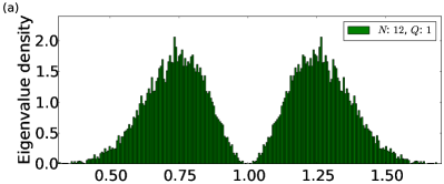
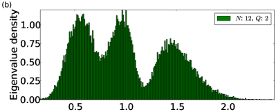
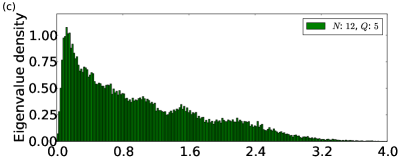
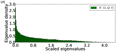
Figure 1: (Color online) The histogram of eigenvalues of the $Q$-qubit reduced density matrix of an $N$-qubit permutation symmetric system. The eigenvalues have been obtained from subsystems of $10000$ randomly generated $N$-qubit permutation symmetric states. The histogram has been scaled such that the area under the curve is one, so that the y-axis is representative of eigenvalue density.

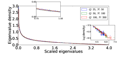
Figure 2: (Color online) The histogram of eigenvalues of the block subsystem for a permutation symmetric system containing (a) $N=50$, (b) $N=100$ and (c) $N=200$ qubits. The eigenvalues have been obtained from $N/2$-qubit subsystems of $2500$ randomly generated $N$-qubit permutation symmetric states, and have been scaled by a factor of $N/2+1$. The histogram has been scaled such that the area under the curve is one, so that the y-axis is representative of eigenvalue density. The Marchenko-Pastur distribution (black line) has been plotted for comparison. The rightmost inset shows the logarithm of the density in the tail region, indicating an exponentially decaying tail.

III.1 Average purity and linear entropy

The superscript label in $\rho^{PS}_{Q}$ is now dropped for brevity. The easiest nontrivial quantity that maybe found for the ensemble is its average purity $\langle\mbox{Tr}\rho_{Q}^{2}\rangle_{PS}$ and hence the average linear entropy $\langle S_{Q}^{l}\rangle_{PS}=1-\langle\mbox{Tr}\rho_{Q}^{2}\rangle_{PS}$. Here $\rho_{Q}=A_{Q}A_{Q}^{\dagger}$, where $A_{Q}$ is from the random ensemble as described in Eq. (13) and Eq. (12), while $\langle\,\cdot\,\rangle_{PS}$ indicates averaging with respect to this “permutation symmetric” ensemble.

$$\langle\mbox{Tr}\rho_{Q}^{2}\rangle_{PS}=\left\langle\sum_{i=1}^{Q+1}\lambda_{i}^{2}\right\rangle_{PS}=\sum_{k,j=0}^{Q}\binom{Q}{k}\binom{Q}{j}\sum_{m,n=0}^{N-Q}\binom{N-Q}{m}\binom{N-Q}{n}\dfrac{\langle a_{k+m}a_{j+n}a^{*}_{k+n}a^{*}_{j+m}\rangle}{\sqrt{\binom{N}{k+m}\binom{N}{j+n}\binom{N}{k+n}\binom{N}{j+m}}}.$$ (16)

If the $a_{i}$ are drawn from the distribution Eq. (12) it is easy to see that $\langle|a_{i}|^{2}|a_{j}|^{2}\rangle=1/[(N+1)(N+2)]$ if $i\neq j$ and is $2/[(N+1)(N+2)]$ if $i=j$. These are the only non-zero average terms that are needed to show that

$$\langle a_{k+m}a_{j+n}a^{*}_{k+n}a^{*}_{j+m}\rangle=\dfrac{1}{(N+1)(N+2)}\left(\delta_{mn}+\delta_{kj}\right).$$ (17)

Using this, the average purity becomes,

$$\begin{split}\langle\mbox{Tr}\rho_{Q}^{2}\rangle_{PS}&=\dfrac{1}{(N+1)(N+2)}\left[\sum_{k,j,m}\dfrac{\binom{Q}{k}\binom{Q}{j}\binom{N-Q}{m}^{2}}{\binom{N}{k+m}\binom{N}{j+m}}\right.\\ &+\left.\sum_{k,m,n}\dfrac{\binom{Q}{k}^{2}\binom{N-Q}{m}\binom{N-Q}{n}}{\binom{N}{k+m}\binom{N}{k+n}}\right].\end{split}$$ (18)

Apparently intimidating, the combinatorial sums are in fact benign, the first is

$$\sum_{k,j,m}\dfrac{\binom{Q}{k}\binom{Q}{j}\binom{N-Q}{m}^{2}}{\binom{N}{k+m}\binom{N}{j+m}}=\dfrac{(N+1)^{2}}{(N-Q+1)},$$ (19)

and the second follows on replacing $Q$ with $N-Q$. Hence finally

$$\begin{split}\langle\mbox{Tr}\rho_{Q}^{2}\rangle_{PS}=\dfrac{N+1}{(Q+1)(N-Q+1)},\\ \langle S^{l}_{Q}\rangle_{PS}=\dfrac{Q(N-Q)}{(Q+1)(N-Q+1)}.\end{split}$$ (20)

To reiterate, the above is the average $Q$ qubit purity and linear entropy of random $N$ qubit permutation symmetric pure states. As expected, it is symmetric under the replacement $Q\rightarrow N-Q$ .

Comparing with the Wishart ensembles, it is known Lubkin (1978) that the average purity of a $M$ dimensional system in a $MN$ dimensional random pure state is $(M+N)/(1+MN)$. Using this we get

$$\begin{split}\langle S_{Q}^{l}\rangle_{W,2^{Q}}=\dfrac{(2^{Q}-1)(2^{N-Q}-1)}{2^{N}+1},\\ \langle S_{Q}^{l}\rangle_{W,Q+1}=\dfrac{Q(N-Q)}{1+(Q+1)(N-Q+1)}.\end{split}$$ (21)

It is understandable that the second ensemble $W,Q+1$ is close in entropy to that of permutation symmetric states. That it is slightly smaller than that of permutation symmetric states is consistent with the behaviour of the density of eigenvalues. While the one for the $W,Q+1$ ensemble is the Marchenko-Pastur one that diverges at the origin and is sharply cut-off at $x=\lambda(Q+1)=4$, the PS ensemble seems to not diverge at the origin and extends to infinity with an exponential tail.

One quantity frequently used in previous studies is $S^{l}_{1}$, that is the linear entropy of a single qubit Wang et al. (2004); Madhok et al. (2015a). In this case:

$$\begin{split}\langle S_{1}^{l}\rangle_{PS}=\frac{1}{2}\left(1-\frac{1}{N}\right),\\ \langle S^{l}_{1}\rangle_{W,2^{Q}}=\frac{1}{2}\left(1-\frac{3}{2^{N}+1}\right),\\ \langle S^{l}_{1}\rangle_{W,Q+1}=\frac{1}{2}\left(1-\frac{3}{2N+1}\right).\end{split}$$ (22)

Thus while both for permutation symmetric as well as asymmetric random states the average of the linear entropy single qubit density matrix approaches the thermalized value of a most mixed state ($=1/2$), the approach is algebraic in the number of qubits for the permutation symmetric states while it is exponential for the asymmetric states if it is assumed to be a $Q$ qubit subsystem.

For the case of $N=2Q$ we have for large $N$:

$$\langle S_{N/2}^{l}\rangle_{PS}\approx 1-\frac{4}{N},\,\langle S_{N/2}^{l}\rangle_{W,2^{Q}}\approx 1-\frac{2}{2^{N/2}},$$ (23)

again illustrating the algebraic rate of scaling to maximum entropy as compared to an exponential one for $Q$ qubits. The case of a $Q+1$ dimensional subsystems of a random state ($W,Q+1$) has the same leading order deviation from $1$ as the PS states. At this level for large $N$ and $N=2Q$ the linear entropies are indistinguishable. The differences however can be seen in quantities like the von Neumann entropy to which we turn to now.

III.2 Average von Neumann entropy

While the linear entropy is easy to calculate and find the average of, it is not additive, and in fact the von Neumann entropy has the special place as the measure of entanglement. In the absence of a j.p.d.f of the eigenvalues of the reduced density matrix or other features of the ensemble, we resort to numerical methods for this quantity. One thing that can be definitely said is that $S^{vN}_{Q}\leq\log(Q+1)$, as the rank of the reduced density matrix is at most $Q+1$ (The logarithms used in the paper are in base 2.) In sharp contrast, for random non-symmetric states, the von Neumann entropy is bounded by $Q$ and the average differs from this by utmost an order 1 number.

Extensive numerical calculations support the following simple formula

$$\begin{split}\langle S^{vN}_{Q}\rangle_{PS}=-\left\langle\sum_{i=1}^{Q+1}\lambda_{i}\log\lambda_{i}\right\rangle_{PS}\\ \approx\log(Q+1)-\alpha\frac{Q+1}{N-Q+1}\end{split}$$ (24)

where $1\leq Q\leq N/2$, $1\ll N$ and $\alpha\approx 2/3$ is a constant. The leading order correction to this seems to be $1/(N+1)$ for the case of $Q=N/2$, and Fig.  3 gives the numerical evidence supporting this claim. Numerically computed average von Neumann entropy and the approximate formula given in Eq. (24) for a $Q$-qubit subsystem of an $N$-qubit permutation symmetric system match quite well.

It is of interest to see how close is the entropy for permutation symmetric states to that of random states in a $(Q+1)\times(N-Q+1)$ dimensional space, namely the $W,Q+1$ ensemble. Using the large $N$ approximation again with $N=2Q$ yields, using a formula first conjectured by Page Page (1993) and proved thereafter Sen (1996); Foong and Kanno (1994); Sánchez-Ruiz (1995)

$$\langle S^{vN}_{Q}\rangle_{W,Q+1}\approx\log(Q+1)-\frac{1}{2\ln 2}\approx\log(Q+1)-0.721.$$ (25)

Comparing with Eq. (24) implies that $\langle S^{vN}_{Q}\rangle_{W,Q+1}$ is marginally smaller than that the random permutation symmetric case, whose average is $\approx 0.66$ smaller that the maximum entanglement. This is seen in Fig.  3 as the systematic lower entropy for the $W,Q+1$ case, which is consistent with the lower linear entropy.

In contrast for random states of $N$ qubits without any symmetry, the $W,2^{Q}$ case,

$$\langle S^{vN}_{Q}\rangle_{W,2^{Q}}\approx Q-\frac{1}{\ln 2}\frac{2^{Q}}{2^{N-Q+1}}.$$ (26)

Thus permutation symmetric states have marginal entanglement that scales with system size in a logarithmic manner. This has been known for some time using different approaches and in Dicke states Popkov and Salerno (2005), but in the context of random states this has not been studied before. It is interesting to note that the asymmetric random states follow a “volume” law while permutation symmetric states are marginal and increase logarithmically with the subsystem size, similar to critical spin chains and integrable CFTs Vidal et al. (2003); Latorre et al. (2005); Popkov et al. (2005); Popkov and Salerno (2005); Barthel et al. (2006); Vidal et al. (2007), and subsequently this affects the behaviour of mutual information Wilms et al. (2012). This has implications for the sign of the tripartite mutual information as we now discuss.

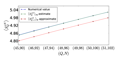
Figure 3: (Color online) A comparison between numerically computed average von Neumann entropy and the approximate formula given in Eq. (24) (along with $1/(N+1)$ correction) for a $Q$-qubit subsystem of an $N$-qubit permutation symmetric system. It can be seen that the approximate formula (green line) matches reasonably well with the numerically computed average (blue line), in contrast with the approximation (Eq. 25) obtained from Page formula (red line). The numerical values have been obtained by averaging over $10000$ random permutation symmetric states.

III.3 Tripartite mutual information

With the above, it is possible to estimate the behaviour of TMI in random permutation symmetric states as well as the Wishart ensemble of $2^{N}$ qubits. Using the definition of the TMI in Eq. (1) it follows that

$$\begin{split}&\left\langle I_{3}(Q,Q,Q)\right\rangle_{PS}\approx 3\log(Q+1)-3\log(2Q+1)\\ &+\log(3Q+1)=\log\left[\frac{(3Q+1)(Q+1)^{3}}{(2Q+1)^{3}}\right]>0,\end{split}$$ (27)

where we have simply used $S_{A}\approx\log(Q+1)$ and ignored corrections. This is sufficient to show that the TMI average value for random permutation symmetric states is positive. The above will be a good approximation only for large $Q$ and $N$.

For the case of the ensemble of all random states on the full $2^{N}$ dimensional space, using the leading order term in Eq. (26) gives for the TMI $3Q-6Q+3Q=0$ and therefore it is necessary to use the deviation from maximally entangled states in that formula and this yields

$$\left\langle I_{3}(Q,Q,Q)\right\rangle_{W,2^{Q}}\approx-\frac{2^{2Q-N-1}}{\ln 2}\left(2^{4Q}-3\,2^{2Q}+3\right).$$ (28)

This is negative as $x^{2}-3x+3\geq 3/4$. This is again valid for large $Q$ and $N$. Therefore typical states are not only entangled but they also have a negative TMI implying that information is distributed in multipartite ways. In contrast for permutation symmetric states, the entanglement is small, being only logarithmic in the number of qubits and hence the TMI is typically positive and the information is stored more in bipartite partitions and is not spread out. We can observe this numerically in Fig. 4, where we compute TMI for subsystems of random states with and without permutation symmetry.

Often it is easier for calculations to use the linear entropy and hence we define, even if a little dubious, a linear entropic TMI by using for $H(\cdot)$ in Eq. (1) the linear entropies. Hence using Eq. (20) we can get exact average linear entropic TMI, for example

$$\left\langle I_{3}^{l}(1,1,1)\right\rangle_{PS}=\frac{(N-3)(N^{2}-N+4)}{4(N-2)N(N-1)}\approx\frac{1}{4}-\frac{1}{4N},$$ (29)

and

$$\left\langle I_{3}^{l}(m,m,m)\right\rangle_{PS}\approx\frac{6m^{3}}{(m+1)(2m+1)(3m+1)}.$$ (30)

These demonstrate again that the TMI of permutation symmetric states, now with the linear entropy, is also positive on the average. However this is not quite useful as it is easy to check that it is also positive for random states that are not symmetric, that is when the reduced density matrix is from the Wishart ensemble. Additivity of the entropy is an important property and as the linear entropy is not additive, it does not distinguish the ensembles. We have verified for example that the Rényi entropy, which is additive at any order, does in fact have the capability.

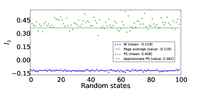
Figure 4: (Color online) TMI ($vN$) between $1$ qubit, $2$ qubit, $2$ qubit subsystem of a $12$ qubit system. The blue points show the TMI for different realizations of asymmetric random states, and it can be seen that the average obtained from Page formula (blue line) matches with the numerical average. The green triangles, on the other hand, show TMI for different realizations of random PS states, and the average TMI obtained from Eq. (24) is moderately close to the numerical average.

In the preceding discussion, we noted that a positive value for average TMI is observed for the PS ensemble. This statement can in fact be extended to cover individual (random) states by the use of Lévy’s lemma. In Appendix B, we show how to apply Lévy’s lemma to permutation symmetric systems so that the average of the quantities we are interested in is taken only over random PS states and not asymmetric states. Using this, we can easily see that for a large number of qubits in the total system, the TMI (based on either von Neumann or linear entropy) for most random PS states is nearly equal to the average TMI. Thus if the average TMI is positive, we can expect most states to have a positive TMI as well, given that we are working in large enough dimensions.

Now, from Eq. (1), we can see that a positive TMI implies that $I_{2}(A:B)+I_{2}(A:C)>I_{2}(A:BC)$, which would mean that the (bipartite) mutual information is not monogamous. Monogamy of an information measure refers to the ability of a party to share correlations, as defined by this measure, with other parties. Our results, therefore, suggest connections between mutual information in permutation symmetric systems and monogamy. More precisely, if we start with a pure permutation symmetric state $\left|\psi_{ABCD}\right\rangle$ corresponding to some partition $ABCD$, the mutual information that $A$ shares individually with the subsystems $B$ and $C$ is greater than what it shares with the joint system $BC$. Thus, the subsystems can share correlations with other parties. Since the mutual information is a measure of total correlations, the correlations that can be shared may either be classical or quantum.

IV Mutual informations and entanglement in the kicked top

We now turn to the details of the kicked top propagator, evolve states using this and explore how in the chaotic regime the random state values of the previous section holds. In the process we study the short time evolution and growth of several interesting measures, the mutual information, the tripartite mutual information, the entanglement and the out-of-time-ordered correlator.

IV.1 The kicked top as a many-body spin model

The kicked top consists of a single large rotor whose quantum evolution over one time period $\tau$ of the kicking is given by the propagator Haake (1991)

$$U=\exp\left(-i\frac{k}{2j}J_{z}^{2}\right)\exp\left(-ipJ_{y}\right)$$ (31)

Since $[\bm{J}^{2},J_{i}]=0$, we are restricted to a $(2j+1)$-dimensional Hilbert space, and we can use the standard angular momentum basis $\{\left|j,m\right\rangle|-j\leq m\leq j\}$, which are the simultaneous eigenstates of $\bm{J}^{2}$ and $J_{z}$. Here $k$ and $p$ are parameters. The classical map Haake (1991); Kuś et al. (1987); Kus et al. (1988); Zyczkowski (1990) is from the surface of the sphere $(J_{x}^{2}+J_{y}^{2}+J_{z}^{2})/j^{2}=1$ into itself. It can have regular as well as chaotic dynamics, and this behaviour is controlled by $k$. We use $p=\pi/2$ below, for which $k=0$ is integrable, being simply a rotation about the $y$ - axis, while around $k=3$ the phase space is a mixed one, with a measure of chaotic and regular trajectories, while for $k=6$ is almost fully chaotic.

The mapping between the kicked top model and the dynamics of qubits allows us to study the kicked top as a many-body system Wang et al. (2004); Madhok et al. (2015b); Neill et al. (2016); Madhok et al. (2018). Since $\bm{J^{2}}$ is conserved, the state of the system can by mapped to a $2j$-qubit (or equivalently, spin-half) system, with the additional constraint that the qubits are always permutation symmetric. The existence of such a mapping can be understood from the fact that permutation symmetry effectively reduces the dimension of the $2j$-qubit system from $2^{2j}$ to $2j+1$, and thus a linear isomorphism exists from the angular momentum $j$ system to the permutation symmetric $2j$-qubit system. The “natural” basis states for the permutation symmetric $2j$-qubit system are therefore the Dicke states. To be explicit, replacing $J^{x,y,z}$ with $\sum_{l=1}^{2j}\sigma^{x,y,z}/2$, the unitary or Floquet operator of the resultant $2j$ spin system is

$$U=\exp\left(-i\frac{k}{8j}\sum_{l\neq l^{\prime}=1}^{2j}\sigma^{z}_{l}\sigma^{z}_{l^{\prime}}\right)\exp\left(-i\frac{\pi}{4}\sum_{l=1}^{2j}\sigma^{y}_{l}\right),$$ (32)

where the $\sigma^{x,y,z}_{l}$ are the standard Pauli matrices, and an overall phase is neglected.

Thus the spin model can be regarded as a kicked long-range transverse field Ising model which has identical interactions between all pairs of spins. While the nearest neighbor transverse field Ising model, kicked or otherwise, is integrable, (for example see Prosen (2000)) the long-range model can be non-integrable in the thermodynamic limit, which is also the classical limit $j\rightarrow\infty$. Floquet models of many-body spin systems are being actively explored in the literature from many perspectives including many-body localization. Thus the kicked top in this many-body avatar presents an opportunity to study entanglement sharing and other typical questions that have been addressed thus far using many other spin models Amico et al. (2008), besides giving us a simple, if potentially chaotic, thermodynamic limit.

If the state vector of the system after $n$ kicks is $\left|\psi_{n}\right\rangle$, the state after $(n+1)$th kick is given by $\left|\psi_{n+1}\right\rangle=U\left|\psi_{n}\right\rangle$. In order to study the quantum-classical correspondence, one typically takes spin coherent states Glauber and Haake (1976); Puri (2001) as initial states. These states are parameterized by $\theta$ and $\phi$, and are minimum uncertainty states and therefore closest analogs to points on the classical phase space, aiding a quantum-classical comparison. Noting that $\left|j,j\right\rangle$ has minimum $\bm{J}^{2}$ uncertainty (the variance of $\bm{J}^{2}$ goes as $j$), the rest of the minimum uncertainty states are generated by rotating this state using $R(\theta,\phi)=\exp{\left(i\theta(J_{x}\sin(\phi)-J_{y}\cos(\phi))\right)}$, i.e., $\left|\theta,\phi\right\rangle=R(\theta,\phi)\left|j,j\right\rangle$. As a state of qubits this is simply the tensor product of qubit states whose Bloch sphere position is uniformly $(\theta,\phi)$: $|\theta,\phi\rangle=\otimes^{2j}(\cos(\theta/2)|0\rangle+e^{i\phi}\sin(\theta/2)|1\rangle)$.

Starting from such an initial spin coherent state, the time evolved state $U^{n}|\theta,\phi\rangle$ resides in the permutationally invariant subspace of the complete Hilbert space of the $2j$ qubits. If the classical kicked top is in a completely chaotic regime, the quantum one generates pseudo-random states for sufficiently large time $n$ Haake (1991). Viewed as a multi-qubit state, it is in the permutation symmetric subspace and therefore we can expect in this case that the results of the previous section on random permutation symmetric states hold good.

There are two aspects of studying the behaviour of TMI and bipartite correlations like the mutual information and entanglement in permutation symmetric states like the ones generated when the dynamics is governed by the kicked top Hamiltonian. One is the investigation of their temporal behaviour that governs their growth and the other is exploring long-time averages or saturation values that would correspond to ensemble averages such as those calculated from the random permutation symmetric states.

IV.2 Growth of information measures and entanglement

It is of particular interest to probe the dynamical behaviour of these correlations as a function of the initial coherent state localized in the regular or chaotic regions of the kicked top phase space. Unlike initial states localized in regular regions, the long-time evolution of the state under global chaos can be expected to thermalize or equilibrate, and this leads us to the study of ensemble averages. To the best of our knowledge, a study of dynamics of these quantum correlations across arbitrary subsystem decompositions is unexplored and earlier works have largely focused on subsystems consisting of a single or at most two qubits of a multi-qubit kicked top Wang et al. (2004); Madhok et al. (2015a). Moreover, the dynamical behaviour of quantities like entanglement and discord were compared rather qualitatively in the chaotic and regular regimes. We find that the Ehrenfest time plays a crucial role for saturation of many of the measures.

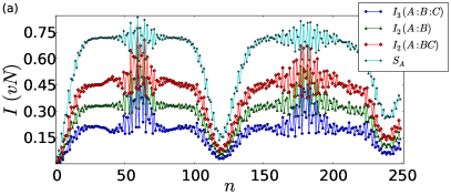
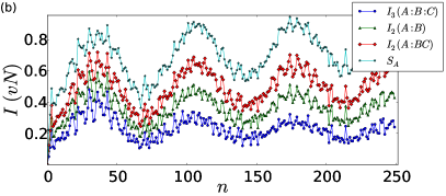
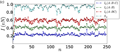
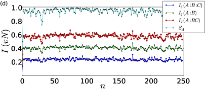
Figure 5: (Color online) TMI, MI and entanglement (computed using von Neumann entropy) between three $1$ qubit subsystems for $j=10$ (i.e., a $20$ qubit system) in the kicked top. The TMI has been obtained in (a) the regular region with $k=1$, $\phi=0.63$, (b) a point in the regular island of the mixed phase space for $k=3$, $\phi=0.63$, (c) a point in the chaotic sea of the mixed phase space for $k=3$, $\phi=2$, and (d) the globally chaotic region with $k=6$, $\phi=0.63$ (in each case, $p=\pi/2$ and $\theta=2.25$). It can be seen that the TMI reflects the regular nature of the underlying classical dynamics.

In accordance with this idea, we plot the behaviour of TMI with time in the kicked top in regular, mixed and chaotic regimes (see figure 5). One would notice right away that the extent of regularity of the classical dynamics bears its signatures on the TMI. Regular dynamics leads to oscillatory TMI with large time variations and large values. In particular $I_{3}(1,1,1)$ is shown for an initial coherent state in a 20 qubit system. When $k=1$ the dynamics is regular and we see large positive values of the TMI indicating that information is shared more in a bipartite manner than collectively. When $k=3$ the dynamics is that of a mixed phase space and starting from a regular region leads to large oscillations of the TMI that seems to be damping over very long time scales. At the same value of $k$, starting from an initial state localized in a region in which the classical limit is chaotic, leads to a rapid growth and saturation of the TMI with small oscillations around $0.234$. Comparing this to the corresponding average TMI ($vN$) for random permutation symmetric states, which is $\approx 0.245$, corroborates our expectation that chaos in the kicked top thermalizes the initially coherent state, making it similar to a random PS state.

A similar situation arises when $k=6$ when the classical map is essentially globally chaotic, only the rise is even faster and the fluctuations smaller. It is this growth rate in a regime of global chaos that is examined further. Figure 6 compares the growth of TMI with that of mutual information and entanglement computed using von Neumann entropy as well as linear entropy for $j=750$ (i.e, $1500$ qubit system), with each of the subsystems containing $100$ qubits each. To put the growth of TMI seen in this figure in perspective, we estimate the Ehrenfest time which is given as

$$t_{\text{Ehrf}}\sim\ln\left(h_{\text{eff}}^{-1}\right)/\lambda_{cl}=\ln(2j+1)/\lambda_{cl},$$ (33)

where the effective Planck’s constant $h_{\text{eff}}$ goes as inverse dimension and $\lambda_{cl}$ is the classical Lyapunov exponent of the underlying system.

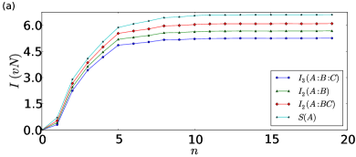
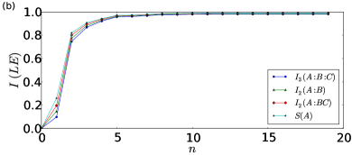
Figure 6: (Color online) TMI, MI and entanglement between three $100$ qubit subsystems for $j=750$ (i.e., a $1500$ qubit system) in the kicked top using (a) von Neumann entropy and (b) linear entropy. It can be seen that the bipartite mutual information and entanglement qualitatively behave like the TMI.

The Lyapunov exponent for the classical kicked top map for $k=6$ is approximately $0.97$, and for $j=750$, we get an Ehrenfest time of approximately $7.54$ time steps. It is evident from figure 6 that the mutual information and TMI grow over the Ehrenfest time. We also see that behaviour of the bipartite mutual informations $I_{2}(A:B)$ and $I_{2}(A:BC)$, entanglement and the TMI are qualitatively alike. While we have shown this for subsystems containing equal number of qubits, this seems to be true even otherwise.

This implies, therefore, that the information between the subsystems $A$ and $B$ (or between $A$ and the joint subsystem $BC$) is similar to the information shared jointly by $A$, $B$ and $C$. Also, the entanglement grows in the same way. One possible reason for such a behaviour could be that the total state of the kicked top grows during the Ehrenfest time due to the effect of underlying classical dynamics, and this total state is what is mapped to a PS system of qubits. This growth, therefore, is reflected in the reduced density matrices obtained from this PS state and the measures computed from these. For such time varying scenarios in PS systems, one therefore needs to re-evaluate the significance of the TMI, as the information provided by TMI is also given by mutual information or even entanglement.

The TMI is defined with the entropies being the additive von Neumann entropy. It appears that the TMI (or mutual information) approaches the saturation value with an exponential rate. We note this by plotting the $\log$ behaviour of the TMI with the saturation value subtracted (not shown here). However, a more careful analysis is required for ascertaining the behaviour of TMI during the growth, and for quantifying the corresponding growth rates.

IV.3 Out-of-time-ordered correlators

The scrambling of localized information in many-body systems is being studied and out-of-time-ordered correlators are used to characterize these Maldacena et al. (2016); Shenker and Stanford (2014); Hayden and Preskill (2007); Hosur et al. (2016). It is convenient to define these via growth of commutators. As we wish to remain in the permutation symmetric subspace, the operators we choose are also permutation invariant and not local. However, it is interesting to study this as it is a simple model of quantum chaos with a well-understood classical limit. For example this was studied in the kicked rotor in Rozenbaum et al. (2017), and there also has been a proposal to investigate scrambling experimentally using the kicked top Swingle et al. (2016).

While postponing a detailed discussion to another work, we wish to contrast and compare this growth with that of the measures discussed above. Define,

$$\begin{split}&F(n)=-\mbox{Tr}[J_{x}(0),J_{x}(n)]^{2}=2\left(C_{2}(n)-C_{4}(n)\right),\\ &C_{2}(n)=\mbox{Tr}(J^{2}_{x}(n)J^{2}_{x}(0)),\\ &C_{4}(n)=\mbox{Tr}(J_{x}(n)J_{x}(0)J_{x}(n)J_{x}(0)),\end{split}$$ (34)

where $J_{x}(n)=U^{-n}J_{x}(0)U^{n}$ and $C_{2}(n)$ is a two-point correlator while $C_{4}(n)$ is the 4-point OTOC and its decrease with time essentially contributes to the growth of the commutator. The $C_{2}(n)$ behaviour is one of fast relaxation within a “diffusion time” Maldacena et al. (2016). In figure 7 we plot these three quantities (usual plot and semi-log plot) for $j=750$, $k=6$, $p=\pi/2$ and see exponential growth in $F(t)$. It is interesting that there are oscillations in $C_{2}(n)$ and $C_{4}(n)$ initially that compensate and lead to an exponential increase in the commutator.

The rate of growth of $F(t)$ seems to be slightly higher ($\approx 2.5$) than the estimate from simply replacing the commutator by classical Poisson brackets and estimating their growth rate at twice the Lyapunov exponent ($\approx 1.94$). On comparing with the other measures such as entanglement of a block of qubits, or TMI in Fig. 6 we see that the Ehrenfest time is the log-time during which the commutator increases exponentially, and then saturates rather quickly.

Thus while there is an exponential growth of the commutators and hence “scrambling”, it seems to be at variance with the positive TMI observed above. Of course there is chaos, and mixing in the classical limit of the kicked top. The resolution maybe in the fact that there is scrambling in phase-space but not in qubit-space. Initial coherent state, localized in phase-space, spreads out exponentially and scrambles in the sense of becoming nonlocal in phase- space, however when viewed as scrambling within the qubits that comprise the effective spin model there is none. This dichotomy is also a reflection of the strong statistical properties, such as spectral fluctuations and eigenvector statistics, of the kicked-top when viewed as a map on the sphere and a single large spin, compared to the marginal entanglement present in subsystems when viewed as collections of qubits.

There is however an effect or reflection of the scrambling in the qubit space. Not in the sign of the TMI but in terms of equilibration of the measures such as entanglement and tripartite mutual information to values that are given by random symmetric ensembles. More importantly, for sufficiently large subsystems, these grow over a log-time $\sim\log(N)$. If there is no chaos we see a much slower growth of these quantities and while more detailed studies are needed, the time-scale seems to be as large as the Heisenberg time $\sim N$, see Fig. (5).

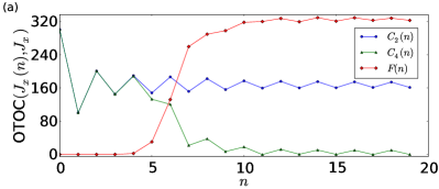
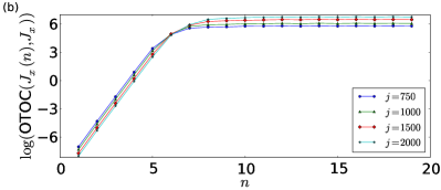
Figure 7: (Color online) (a) $F(n)$, $C_{2}(n)$ and $C_{4}(n)$ for $j=750$, $k=6$, $p=\pi/2$. The OTOC value has been divided by $j^{4}$ to normalize (or equivalently, the operators are being normalized by $j$). (b) Semi-log plot of OTOC for $j=750,1000,1500,2000$ and $k=6$.

IV.4 Saturation and long-time averages

In addition to the dynamical behaviour, we also study the time-averaged TMI in the kicked top. We have already noted that the signature of classical dynamics is present in the time-varying TMI. Figure 8 shows that such a behaviour is also present when we take time averages of TMI. In particular, comparing this figure with figure 9, we can see that classical structures leave their mark on the quantum system, with regular islands being visible for integrable regimes, and low-period periodic orbits being present for the chaotic regimes. The latter is also a result of eigenfunction scarring Heller (1984).

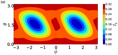
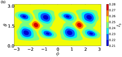
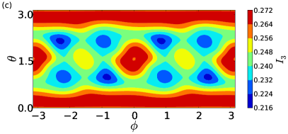
Figure 8: (Color online) Time-averaged TMI between three one qubit subsystems for $j=6$ ($12$ qubits) and $p=\pi/2$, with the initial state corresponding to a coherent stated associated with a $50\times 100$ grid discretizing $\theta\in[0,\ \pi)$ and $\phi\in[0,\ 2\pi)$. The time-averaged TMI is obtained for (a) $k=1$ corresponding to a classically regular region, (b) $k=3$, a mixed regime and (c) $k=6$, a globally chaotic region, and is computed by averaging over $1000$ iterations starting from the initial coherent state. It can be that the classical structures are reproduced to a certain extent.

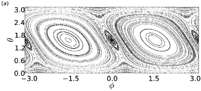
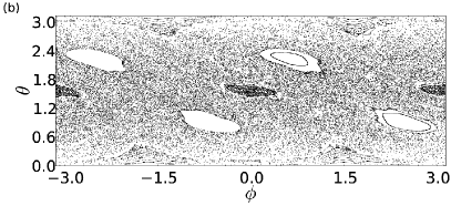
Figure 9: Phase portrait of the classical kicked top map, showing (a) globally regular dynamics for $k=1$, (b) a mixed dynamics with coexisting regions of chaoticity and regularity for $k=3$ and (c) (almost) globally chaotic dynamics for $k=6$. $p=\pi/2$ is used in all the cases.

One can note, in particular, that the average TMI for a large number of points in the phase space is positive. This is true not only in the globally chaotic region, but also in the mixed and regular regimes. In the globally chaotic case, we can see that the average TMI varies approximately from $0.22$ to $0.27$, while the average TMI obtained from random PS states for the corresponding case is $\approx 0.24$. As before, this indicates that chaotic evolution nearly transforms the initially coherent states to random PS states.

V Summary and discussion

In this paper, multi-qubit permutation symmetric states have been studied in general. An algorithm for getting the reduced density matrix of any number of qubits is given. This lead to the definition of a new random matrix ensemble that is of relevance in such cases, the random permutation symmetric states. It has been shown that the distribution of the eigenvalues of the reduced density matrices of this ensemble, while similar to the Marchenko-Pastur is also different in crucial features and defines a new universality class.

For such a random ensemble we have derived analytical expressions for the average purity and linear entropy of arbitrary subsystems and approximate expressions for the average von Neumann entropy. In particular random permutation symmetric states have an “area-law” kind of entanglement scaling only as $\log$(number of qubits in the subsystem). This small multipartite entanglement effectively results in positive tripartite mutual information, for which we derive analytical estimates. In comparison we point out that random states with no symmetry would have a typical TMI value that is negative.

We applied these general statements to a qubit model of the kicked top which can show a range of dynamical behaviour from the regular to the fully chaotic. An interesting aspect that has been recently investigated in certain quantum chaotic systems is the notion of scrambling of information, which refers to the delocalization with time of initially localized information across the system. Both OTOC and TMI have been proposed as a measure to detect scrambling of information, wherein a growth/decay of the OTOC or a negative value of TMI are considered as signatures of scrambling. In our analysis of the kicked top, we observe that OTOCs defined with observables on phase space grow exponentially fast with time (within the Ehrenfest time), while as noted above, permutation symmetry in the system is responsible for most states having a positive value of TMI. Thus the quantum chaos in this case results in scrambling in phase-space while remaining unscrambled in qubit-space.

While Iyoda and Sagawa have also pointed out that TMI for certain initial states are positive Iyoda and Sagawa (2017), they argue that the effective dimension of the set of such states is small. If we consider the qubit model of the kicked top, the permutation symmetric subspace that we are restricted to is only $N+1$ of the total $2^{N}$ dimensional one, and is therefore consistent with their observations. It will be interesting to explore the model in the non-permutation symmetric subspace when it may not have an interpretation as a kicked top. Nevertheless it is likely that the same parameter regimes lead to strongly chaotic behaviour, negative TMI and exponentially growing OTOC. We are also hopeful that our observations about permutation symmetric states will be of broad applicability.

Note added: Along with the present study, another work appeared Pappalardi et al. (2018) which investigates scrambling in long-range spin chains, including the case of kicked top.

Appendix A Subsystems of Permutation Symmetric Systems

In section II, we saw that the structure of Dicke states can be used to write permutation symmetric vectors of $N$ qubits in terms of tensor product of permutation symmetric vectors containing $Q$ and $N-Q$ qubits ($Q<N$). Equation 5 holds, however, only when the vectors are viewed as elements of the full $2^{N}$ dimensional space. We can nevertheless use the idea presented in Eq. (5) to work with permutation symmetric systems without viewing them as subspace of a larger space. An apparent tradeoff of working exclusively with permutation symmetric spaces is that the tensor product structure would be lost, as an $N+1$ dimensional space in general cannot be written as a tensor product of $Q+1$ and $N-Q+1$ dimensional spaces. Fortunately though, it is still possible to work conveniently with subsystems. We show in the following that we can embed a permutation symmetric vector of $N$ qubits into the tensor product of $Q$ qubit and $N-Q$ qubit permutation symmetric spaces such that inner products are preserved.

Proposition 1.

For $d_{X},d_{Y},d_{Z}\in\mathbb{N}$, let $\{\left|i_{X}\right\rangle\ |\ 0\leq i\leq d_{X}\}$ be some fixed orthonormal basis of $X$, $\{\left|j_{Y}\right\rangle\ |\ 0\leq j\leq d_{Y}\}$ be a fixed orthonormal basis of $Y$ and $\{\left|k_{Z}\right\rangle\ |\ 0\leq k\leq d_{Z}\}$ be a fixed orthonormal basis of $Z$, such that $d_{X}=d_{Y}+d_{Z}$. Then the map

$$\iota\colon X\to Y\otimes Z$$

$$\iota\left(\sum_{i=0}^{d_{X}}a_{i}\left|i_{X}\right\rangle\right)=\sum_{j=0}^{d_{Y}}\sum_{k=0}^{d_{Z}}A_{jk}\left|j_{Y}\right\rangle\left|k_{Z}\right\rangle$$

$$\text{with }A_{jk}=C_{jk}a_{j+k}=\sqrt{\frac{\binom{d_{Y}}{j}\binom{d_{Z}}{k}}{\binom{d_{X}}{j+k}}}a_{j+k}$$

is linear and injective. Further, the map is isometric (i.e., preserves inner products).

Proof.

That the map is linear is clear. To see that it is injective, note that if $\iota(\left|a_{X}\right\rangle)=0$ for some $\left|a_{X}\right\rangle\in X$, then each of the coefficients $A_{jk}$ are zero. Thus $a_{i}=0$ implying $\left|a_{X}\right\rangle=0$ (i.e., the kernel of $\iota$ is trivial), establishing the injectivity of $\iota$. Showing isometry of $\iota$ involves a simple computation using Vandermonde Convolution identity.

Towards this end, say $\left|a_{X}\right\rangle=\sum_{i}a_{i}\left|i_{X}\right\rangle$ and $\left|b_{X}\right\rangle=\sum_{i}b_{i}\left|i_{X}\right\rangle$, so that $\left\langle\left|a_{X}\right\rangle,\left|b_{X}\right\rangle\right\rangle=\sum_{i}a_{i}^{*}b_{i}$. On the other hand, $\left\langle\iota(\left|a_{X}\right\rangle),\iota(\left|b_{X}\right\rangle)\right\rangle=\sum_{j}\sum_{k}A_{jk}^{*}B_{jk}=\sum_{j}\sum_{k}C_{jk}^{2}a_{j+k}^{*}b_{j+k}$. Now the sum over $0\leq j\leq d_{Y}$ and $0\leq k\leq d_{Z}$ is done along the “cross-diagonals” $j+k=r$. That is fix an $r$ ($0\leq r\leq d_{X}=d_{Y}+d_{Z}$) and sum over $\max(0,r-d_{Z})\leq j\leq\min(r,d_{Y})$, and do this for all $0\leq r\leq d_{X}$.

$$\left\langle\iota(\left|a_{X}\right\rangle),\iota(\left|b_{X}\right\rangle)\right\rangle =\sum_{r=0}^{d_{X}}\frac{a_{r}^{*}b_{r}}{\binom{d_{X}}{r}}\sum_{j=\max(0,r-d_{Z})}^{\min(r,d_{Y})}\binom{d_{Y}}{j}\binom{d_{Z}}{r-j}$$

$$=\sum_{r=0}^{d_{Z}}\frac{a_{r}^{*}b_{r}}{\binom{d_{X}}{r}}\sum_{j=0}^{\min(r,d_{Y})}\binom{d_{Y}}{j}\binom{d_{Z}}{r-j}$$

$$+\sum_{r=d_{Z}+1}^{d_{X}}\frac{a_{r}^{*}b_{r}}{\binom{d_{X}}{r}}\sum_{j=0}^{d_{X}-r}\binom{d_{Y}}{j}\binom{d_{Z}}{d_{X}-r-j}$$

$$=\sum_{r=0}^{d_{Z}}\frac{a_{r}^{*}b_{r}}{\binom{d_{X}}{r}}\binom{d_{X}}{r}+\sum_{r=d_{Z}+1}^{d_{X}}\frac{a_{r}^{*}b_{r}}{\binom{d_{X}}{r}}\binom{d_{X}}{r}$$

(using Vandermonde Convolution)

$$=\sum_{r=0}^{d_{X}}a_{r}^{*}b_{r}$$

$$=\left\langle\left|a_{X}\right\rangle,\left|b_{X}\right\rangle\right\rangle$$

The above assumes that $d_{Y}\leq d_{Z}$, if not, sum over $k$ instead, following the same steps. Thus, $\iota$ is an isometry. ∎

Hence, given an $N$ qubit permutation symmetric state, we can work as if it has a tensor product decomposition in terms of permutation symmetric states of $Q$ and $N-Q$ qubits.

Furthermore, if we were to embed these vectors in the full $2^{N}$ dimensional space (by mapping each basis vector to the appropriate Dicke state), then these are actually the same vector. To elaborate on this point, say given a vector space $V$ of dimension $d_{V}+1$, we define the linear map $\mathcal{E}_{V}$ as one that takes some fixed basis vectors of the space $V$ to the corresponding Dicke states in the $2^{d_{X}}$ dimensional space ($d_{V}\leq d_{X}$).

$$\mathcal{E}_{V}(\left|i_{V}\right\rangle)=\frac{1}{\sqrt{\binom{d_{V}}{i}}}\sum_{\begin{subarray}{c}0\leq l\leq 2^{d_{X}}-1\\ w(l)=i\end{subarray}}\left|l\right\rangle,\ 0\leq i\leq d_{V}$$ (35)

The action on the fixed basis vectors $\left|i_{V}\right\rangle$ can be extended linearly to define $\mathcal{E}_{V}$ on every vector of $V$ (and such an extension is unique). With such a linear map, we can see that the vectors related by the embedding $\iota$ are actually equal in the full $2^{d_{X}}$ dimensional space. In other words, we have $\mathcal{E}_{X}=(\mathcal{E}_{Y}\otimes\mathcal{E}_{Z})\circ\iota$, which is essentially the content of Eq. (5) mentioned in section II.

Now, since we always work in dimensions linear in the number of qubits, one can study permutation symmetric systems with very large number of qubits. In such a scenario, it may be helpful to obtain the combinatorial coefficients appearing in the expression for reduced density matrix recursively. So if $C_{kl}$ are the combinatorial coefficients as defined in proposition 1, we have the following recursion relations for the same.

$$C_{k+1,l} =\sqrt{\left(\frac{Q-k}{N-k-l}\right)}\sqrt{\left(\frac{k+l+1}{k+1}\right)}C_{kl}$$ (36)

$$C_{k,l+1} =\sqrt{\left(\frac{N-Q-l}{N-k-l}\right)}\sqrt{\left(\frac{k+l+1}{l+1}\right)}C_{kl}$$ (37)

$$C_{k+1,l+1} =\sqrt{\left(\frac{Q-k}{N-k-l-1}\right)}\sqrt{\left(\frac{k+l+2}{k+1}\right)}$$ (38)

$$\hskip 22.76228pt\sqrt{\left(\frac{N-Q-l}{N-k-l}\right)}\sqrt{\left(\frac{k+l+1}{l+1}\right)}C_{kl}$$ (39)

Here, in place of $d_{X}$ we have used $N$ and $Q$ in place of $d_{Y}$, which denote the number of qubits in the system and the subsystem respectively. These relations can be used to compute $C_{kl}$ when working with a large number of qubits.

Appendix B Lévy’s Lemma for Permutation Symmetric Systems

Lévy’s lemma is a statement describing the relation between the values taken by a Lipschitz continuous function defined on a sphere and its average with respect to the uniform measure on the sphere. The normalization requirement of quantum states allows us to consider the state as a point on a unit sphere. The work in Hayden et al. (2006) describes the use of Lévy’s lemma in the context of quantum systems. In particular, their study covers the cases of von Neumann and linear entropy for a system of qubits. But if we directly apply their results to a PS system of qubits, the average would correspond to the Wishart ensemble, while we are interested in averages over the PS ensemble. Thus we need to appropriately adapt the relevant proofs presented in Hayden et al. Hayden et al. (2006) to cover the case of PS system of qubits, so that the averages indeed correspond to those over the PS ensemble.

Our starting point is the property noted in Appendix A, that given any $N$ qubit permutation symmetric vector, it has a tensor product decomposition in terms of $Q$ qubit and $N-Q$ qubit permutation symmetric vectors. So, given any permutation symmetric vector $\left|a_{X}\right\rangle\in X$ of dimension $d_{X}+1$ and subsystems $Y$ and $Z$ of dimensions $d_{Y}+1$ and $d_{Z}+1$ respectively (so that $d_{X}=d_{Y}+d_{Z}$), let the map $G\colon X\to\mathcal{L}(Y)$ take this vector to the reduced density matrix of subsystem $Y$. That is,

$$G(\left|a_{X}\right\rangle)=\mbox{Tr}_{Z}\left|\iota(a_{X})\right\rangle\left\langle\iota(a_{X})\right|$$ (40)

where $\iota$ is the embedding defined in Appendix A. We will combine this with the proof of Lipschitz continuity of von Neumann entropy and purity Hayden et al. (2006) to adapt them to the permutation symmetric case. In the following discussion, the Lipschitz continuity of functions is considered with respect to the Euclidean norm.

Proposition 2.

1. The von Neumann entropy is a Lipschitz continuous function for permutation symmetric states. That is, the function $f\colon X\to\mathbb{R}$ defined as

   $$f(\left|a_{X}\right\rangle)=S^{vN}(G(\left|a_{X}\right\rangle))$$

   is Lipschitz continuous with respect to the Euclidean norm for $d_{Y}\geq 2$.

2. The linear entropy is a Lipschitz continuous function for permutation symmetric states.

3. The tripartite mutual information between any three subsystems of a permutation symmetric system is Lipschitz continuous, where the TMI is calculated either using von Neumann or linear entropy. For the case of von Neumann entropy, each of the subsystems must have at least two qubits, and so the total system should have at least six qubits.

Proof.

(i) In Ref. Hayden et al. (2006) it has been shown that given any $\left|\phi_{Y\otimes Z}\right\rangle\in Y\otimes Z$, the function $f^{\prime}\colon Y\otimes Z\to\mathbb{R}$ defined as $f^{\prime}(\left|\phi_{Y\otimes Z}\right\rangle)=S^{vN}(\rho_{Y})$ (where $\rho_{Y}$ is the reduced density matrix of subsystem $Y$) is Lipschitz continuous for $d_{Y}\geq 2$, with the Lipschitz constant bounded above by $\sqrt{8}\log(d_{Y}+1)$. In other words,

$$|f^{\prime}(\left|\phi_{Y\otimes Z}\right\rangle)-f^{\prime}(\left|\psi_{Y\otimes Z}\right\rangle)|\leq$$

$$\sqrt{8}\log(d_{Y}+1))\left\lVert\left|\phi_{Y\otimes Z}\right\rangle-\left|\psi_{Y\otimes Z}\right\rangle\right\rVert_{2}$$

for $d_{Y}\geq 2$, where $\left\lVert\cdot\right\rVert_{2}$ is the Euclidean norm. As this is valid for any vector in $Y\otimes Z$, it is, in particular, valid for $\iota(\left|a_{X}\right\rangle),\ \iota(\left|b_{X}\right\rangle)\in Y\otimes Z$ given any $\left|a_{X}\right\rangle,\ \left|b_{X}\right\rangle\in X$. Noting that $f(\left|a_{X}\right\rangle)=f^{\prime}(\iota(\left|a_{X}\right\rangle)$, we get

$$|f(\left|a_{X}\right\rangle-f(\left|b_{X}\right\rangle)| \leq\sqrt{8}\log(d_{Y}+1)\left\lVert\iota(\left|a_{X}\right\rangle)-\iota(\left|b_{X}\right\rangle)\right\rVert_{2}$$

$$\leq\sqrt{8}\log(d_{Y}+1)\left\lVert\left|a_{X}\right\rangle-\left|b_{X}\right\rangle\right\rVert_{2}$$

(using linearity and isometry of $$\iota$$)

for $d_{Y}\geq 2$. Thus, $f(\left|a_{X}\right\rangle)=S^{vN}(G(\left|a_{X}\right\rangle))$ is Lipschitz continuous with the Lipschitz constant bounded above by $\sqrt{8}\log(d_{Y}+1)$.

(ii) We start by showing that for any $\left|a_{X}\right\rangle\in X$, the function $f(\left|a_{X}\right\rangle)=\sqrt{\mbox{Tr}(G(\left|a_{X}\right\rangle)^{2})}$ is Lipschitz continuous. Again, we resort to the corresponding result for the case $\left|\phi_{Y\otimes Z}\right\rangle\in Y\otimes Z$ in Hayden et al. (2006). In particular, for the function $f^{\prime}\colon Y\otimes Z\to\mathbb{R}$ defined as $f^{\prime}(\left|\phi_{Y\otimes Z}\right\rangle)=\sqrt{\mbox{Tr}(\rho_{Y}^{2})}$, they showed that

$$|f^{\prime}(\left|\phi_{Y\otimes Z}\right\rangle)-f^{\prime}(\left|\psi_{Y\otimes Z}\right\rangle)|\leq 2\left\lVert\left|\phi_{Y\otimes Z}\right\rangle-\left|\psi_{Y\otimes Z}\right\rangle\right\rVert_{2}$$

As before, taking any $\left|a_{X}\right\rangle,\ \left|b_{X}\right\rangle\in X$, we apply the above for $\iota(\left|a_{X}\right\rangle),\ \iota(\left|b_{X}\right\rangle)\in Y\otimes Z$ while noting that $f(\left|a_{X}\right\rangle)=f^{\prime}(\iota(\left|a_{X}\right\rangle))$ to get

$$|f(\left|a_{X}\right\rangle)-f(\left|b_{X}\right\rangle)|\leq 2\left\lVert\left|a_{X}\right\rangle-\left|b_{X}\right\rangle\right\rVert_{2}$$

where we have utilized the linearity and isometry of $\iota$. Now observe that $f$ is bounded above by $1$ since $\mbox{Tr}(\rho^{2})\leq 1$ for any density matrix $\rho$. Thus, $|f^{2}(\left|a_{X}\right\rangle)-f^{2}(\left|b_{X}\right\rangle)|=|f(\left|a_{x}\right\rangle)-f(\left|b_{X}\right\rangle)||f(\left|a_{X}\right\rangle)+f(\left|b_{X}\right\rangle)|\leq 4\left\lVert\left|a_{X}\right\rangle-\left|b_{X}\right\rangle\right\rVert_{2}$, where the triangle inequality, upper bound of $f$ and the above inequality has been used. Therefore, $f^{2}$ is Lipschitz continuous with the Lipschitz constant bounded above by $4$. As the linear entropy corresponding to the state $\left|a_{X}\right\rangle$ is given by $1-f^{2}(\left|a_{X}\right\rangle)$, it is Lipschitz continuous with the Lipschitz constant bounded above by $4$.

(iii) Let $A$, $B$, $C$ with dimensions $d_{A}+1$, $d_{B}+1$ and $d_{C}+1$ respectively be subspaces of the space $X$ with dimension $d_{X}+1$. We abbreviate the space of the joint permutation symmetric systems as follows: $AB$ having dimension $d_{A}+d_{B}+1$, $BC$ having dimension $d_{B}+d_{C}+1$, $AC$ having dimension $d_{A}+d_{C}+1$ and $ABC$ having dimension $d_{A}+d_{B}+d_{C}+1$. Further, these spaces are such that $d_{A}+d_{B}+d_{C}\leq d_{X}$. Now, say $f_{Y}\colon X\to\mathbb{R}$ is either the von Neumann entropy or the linear entropy (corresponding to a given subsystem $Y$). We know that $f_{Y}$ is Lipschitz continuous with the Lipschitz constant bounded above by $\eta_{Y}$, which is equal to $\sqrt{8}\log(d_{Y}+1)$ for the case of von Neumann entropy and equal to $4$ for the case of linear entropy.

Let $f^{TMI}\colon X\to\mathbb{R}$ be defined as

$$f^{TMI}(\left|a_{X}\right\rangle)=f_{A}(\left|a_{X}\right\rangle)+f_{B}(\left|a_{X}\right\rangle)+f_{C}(\left|a_{X}\right\rangle)$$

$$-f_{AB}(\left|a_{X}\right\rangle)-f_{BC}(\left|a_{X}\right\rangle)-f_{AC}(\left|a_{X}\right\rangle)+f_{ABC}(\left|a_{X}\right\rangle)$$

Then for any vectors $\left|a_{X}\right\rangle,\left|b_{X}\right\rangle\in X$, using triangle inequality and the Lipschitz continuity of $f_{Y}$, we get

$$|f^{TMI}(\left|a_{X}\right\rangle)-f^{TMI}(\left|b_{X}\right\rangle)|\leq$$

$$(\eta_{A}+\eta_{B}+\eta_{C}+\eta_{AB}+\eta_{BC}+\eta_{AC}+\eta_{ABC})\left\lVert\left|a_{X}\right\rangle-\left|b_{X}\right\rangle\right\rVert_{2}$$

Therefore $f^{TMI}$ is Lipschitz continuous with the Lipschitz constant bounded above by $\eta=(\eta_{A}+\eta_{B}+\eta_{C}+\eta_{AB}+\eta_{BC}+\eta_{AC}+\eta_{ABC})$. In other words, the TMI defined on permutation symmetric spaces is Lipschitz continuous for either von Neumann entropy or linear entropy. Note that for Lipschitz continuity of von Neumann entropy, we require $d_{Y}\geq 2$ for each of the subsystems. ∎

Now that we have the von Neumann entropy, linear entropy and TMI as Lipschitz continuous functions on permutation symmetric systems, we can resort to Lévy’s lemma. To recall, Lévy’s lemma is stated as follows Hayden et al. (2006).

Lemma 1 (Lévy).

Let $f\colon S^{n-1}\to\mathbb{R}$ be a Lipschitz continuous function (with respect to the Euclidean norm in $\mathbb{R}^{n}$) with a Lipschitz constant $\eta$, where $S^{n-1}$ is a unit sphere in $\mathbb{R}^{n}$. If $x\in S^{n-1}$ is picked randomly (with respect to the uniform measure on the sphere), then for $\epsilon\geq 0$ we have

$$\mathbb{P}\{|f(x)-\mathbb{E}[f]|\geq\epsilon\}\leq 2\exp\left(-\frac{n\epsilon^{2}}{9\pi^{3}\ln(2)\eta^{2}}\right)$$

where $\mathbb{E}[f]$ is the expectation value of $f$ with respect to the uniform measure on the sphere.

Thus, for large enough dimensions, we can say that almost all random permutation symmetric states have von Neumann entropy, linear entropy and TMI close to the respective averages. In particular, a positive average TMI implies that most states also have positive TMI.

References

- Arnol’d and Avez (1968) V. I. Arnol’d and A. Avez, Ergodic problems of classical mechanics (WA Benjamin, 1968).
- Gutzwiller (1990) M. C. Gutzwiller, Chaos in Classical and Quantum Mechanics (Springer-Verlag, New York, 1990).
- Haake (1991) F. Haake, Quantum Signatures of Chaos (Spring-Verlag, Berlin, 1991).
- Gutzwiller (1971) M. C. Gutzwiller, Journal of Mathematical Physics 12, 343 (1971).
- Berry and Tabor (1977) M. Berry and M. Tabor, Proceedings of the Royal Society of London A: Mathematical, Physical and Engineering Sciences 356, 375 (1977).
- Bohigas et al. (1984) O. Bohigas, M.-J. Giannoni, and C. Schmit, Physical Review Letters 52, 1 (1984).
- Robnik and Berry (1985) M. Robnik and M. V. Berry, Journal of Physics A: Mathematical and General 18, 1361 (1985).
- Berry (1977) M. V. Berry, Journal of Physics A: Mathematical and General 10, 2083 (1977).
- Voros (1976) A. Voros, Ann. Inst. Henri Poincaré A 24, 31 (1976).
- McDonald and Kaufman (1979) S. W. McDonald and A. N. Kaufman, Physical Review Letters 42, 1189 (1979).
- Heller (1984) E. J. Heller, Physical Review Letters 53, 1515 (1984).
- Berry et al. (1979) M. Berry, N. Balazs, M. Tabor, and A. Voros, Annals of Physics 122, 26 (1979).
- Åberg (1990) S. Åberg, Physical Review Letters 64, 3119 (1990).
- Montambaux et al. (1993) G. Montambaux, D. Poilblanc, J. Bellissard, and C. Sire, Physical Review Letters 70, 497 (1993).
- Hsu and Angles d’Auriac (1993) T. C. Hsu and J. Angles d’Auriac, Physical Review B 47, 14291 (1993).
- van der Pals and Gaspard (1994) P. v. E. van der Pals and P. Gaspard, Physical Review E 49, 79 (1994).
- Kudo and Deguchi (2003) K. Kudo and T. Deguchi, Physical Review B 68, 052510 (2003).
- Rabson et al. (2004) D. A. Rabson, B. Narozhny, and A. Millis, Physical Review B 69, 054403 (2004).
- Jacquod and Shepelyansky (1997) P. Jacquod and D. Shepelyansky, Physical Review Letters 79, 1837 (1997).
- Georgeot and Shepelyansky (1998) B. Georgeot and D. Shepelyansky, Physical Review Letters 81, 5129 (1998).
- Lakshminarayan and Subrahmanyam (2003) A. Lakshminarayan and V. Subrahmanyam, Physical Review A 67, 052304 (2003).
- Avishai et al. (2002) Y. Avishai, J. Richert, and R. Berkovits, Physical Review B 66, 052416 (2002).
- Santos (2004) L. Santos, Journal of Physics A: Mathematical and General 37, 4723 (2004).
- Kudo and Deguchi (2004) K. Kudo and T. Deguchi, Physical Review B 69, 132404 (2004).
- Lakshminarayan and Subrahmanyam (2005) A. Lakshminarayan and V. Subrahmanyam, Physical Review A 71, 062334 (2005).
- Karthik et al. (2007) J. Karthik, A. Sharma, and A. Lakshminarayan, Physical Review A 75, 022304 (2007).
- D’Alessio et al. (2016) L. D’Alessio, Y. Kafri, A. Polkovnikov, and M. Rigol, Advances in Physics 65, 239 (2016), https://doi.org/10.1080/00018732.2016.1198134 .
- Maldacena and Stanford (2016) J. Maldacena and D. Stanford, Physical Review D 94, 106002 (2016).
- Bohigas and Flores (1971) O. Bohigas and J. Flores, Physics Letters B 35, 383 (1971).
- Kota (2001) V. Kota, Physics Reports 347, 223 (2001).
- Mehta (2004) M. L. Mehta, Random matrices, Vol. 142 (Elsevier, 2004).
- Neill et al. (2016) C. Neill, P. Roushan, M. Fang, Y. Chen, M. Kolodrubetz, Z. Chen, A. Megrant, R. Barends, B. Campbell, B. Chiaro, A. Dunsworth, E. Jeffrey, J. Kelly, J. Mutus, P. J. J. O’Malley, C. Quintana, D. Sank, A. Vainsencher, J. Wenner, T. C. White, A. Polkovnikov, and J. M. Martinis, Nature Physics 12, 1037 (2016).
- Kaufman et al. (2016) A. M. Kaufman, M. E. Tai, A. Lukin, M. Rispoli, R. Schittko, P. M. Preiss, and M. Greiner, Science 353, 794 (2016).
- Miller and Sarkar (1999) P. A. Miller and S. Sarkar, Physical Review E 60, 1542 (1999).
- Lakshminarayan (2001) A. Lakshminarayan, Physical Review E 64, 036207 (2001).
- Bandyopadhyay and Lakshminarayan (2002) J. N. Bandyopadhyay and A. Lakshminarayan, Physical Review Letters 89, 060402 (2002).
- Scott and Caves (2003) A. J. Scott and C. M. Caves, Journal of Physics A: Mathematical and General 36, 9553 (2003).
- Jacquod (2004a) P. Jacquod, Physical Review Letters 92, 150403 (2004a).
- Jacquod (2004b) P. Jacquod, Physical Review Letters 93, 219903 (2004b).
- Petitjean and Jacquod (2006) C. Petitjean and P. Jacquod, Physical Review Letters 97, 194103 (2006).
- Ghose and Sanders (2004) S. Ghose and B. C. Sanders, Physical Review A 70, 062315 (2004).
- Wang et al. (2004) X. Wang, S. Ghose, B. C. Sanders, and B. Hu, Physical Review E 70, 016217 (2004).
- Trail et al. (2008) C. M. Trail, V. Madhok, and I. H. Deutsch, Physical Review E 78, 046211 (2008).
- Madhok et al. (2015a) V. Madhok, V. Gupta, D.-A. Trottier, and S. Ghose, Physical Review E 91, 032906 (2015a).
- Madhok et al. (2014) V. Madhok, C. A. Riofrío, S. Ghose, and I. H. Deutsch, Physical Review Letters 112, 014102 (2014).
- Braunstein et al. (2013) S. L. Braunstein, S. Pirandola, and K. Życzkowski, Physical Review Letters 110, 101301 (2013).
- Hartman and Maldacena (2013) T. Hartman and J. Maldacena, Journal of High Energy Physics 2013, 14 (2013).
- Shenker and Stanford (2014) S. H. Shenker and D. Stanford, Journal of High Energy Physics 2014, 67 (2014).
- Sekino and Susskind (2008) Y. Sekino and L. Susskind, Journal of High Energy Physics 2008, 065 (2008).
- Lashkari et al. (2013) N. Lashkari, D. Stanford, M. Hastings, T. Osborne, and P. Hayden, Journal of High Energy Physics 2013, 22 (2013).
- Maldacena et al. (2016) J. Maldacena, S. H. Shenker, and D. Stanford, Journal of High Energy Physics 2016, 106 (2016).
- Hosur et al. (2016) P. Hosur, X.-L. Qi, D. A. Roberts, and B. Yoshida, Journal of High Energy Physics 2016, 4 (2016).
- Iyoda and Sagawa (2017) E. Iyoda and T. Sagawa, arXiv:1704.04850 (2017).
- Kuś et al. (1987) M. Kuś, R. Scharf, and F. Haake, Zeitschrift für Physik B Condensed Matter 66, 129 (1987).
- Kus et al. (1988) M. Kus, J. Mostowski, and F. Haake, Journal of Physics A: Mathematical and General 21, L1073 (1988).
- Zyczkowski (1990) K. Zyczkowski, Journal of Physics A: Mathematical and General 23, 4427 (1990).
- Emerson et al. (2003) J. Emerson, Y. S. Weinstein, M. Saraceno, S. Lloyd, and D. G. Cory, science 302, 2098 (2003).
- Vidal et al. (2003) G. Vidal, J. I. Latorre, E. Rico, and A. Kitaev, Physical Review Letters 90, 227902 (2003).
- Latorre et al. (2005) J. I. Latorre, R. Orús, E. Rico, and J. Vidal, Physical Review A 71, 064101 (2005).
- Popkov et al. (2005) V. Popkov, M. Salerno, and G. Schütz, Physical Review A 72, 032327 (2005).
- Popkov and Salerno (2005) V. Popkov and M. Salerno, Physical Review A 71, 012301 (2005).
- Barthel et al. (2006) T. Barthel, S. Dusuel, and J. Vidal, Physical Review Letters 97, 220402 (2006).
- Vidal et al. (2007) J. Vidal, S. Dusuel, and T. Barthel, Journal of Statistical Mechanics: Theory and Experiment 2007, P01015 (2007).
- Marčenko and Pastur (1967) V. A. Marčenko and L. A. Pastur, Mathematics of the USSR-Sbornik 1, 457 (1967).
- Madhok et al. (2018) V. Madhok, S. Dogra, and A. Lakshminarayan, Optics Communications 420, 189 (2018).
- Rangamani and Rota (2015) M. Rangamani and M. Rota, Journal of Physics A: Mathematical and Theoretical 48, 385301 (2015).
- Rota (2016) M. Rota, Journal of High Energy Physics 2016, 75 (2016).
- Moreno and Parisio (2018) M. Moreno and F. Parisio, arXiv preprint arXiv:1801.00762 (2018).
- Popkov and Salerno (2012) V. Popkov and M. Salerno, International Journal of Modern Physics B 26, 1243009 (2012).
- Markham (2011) D. J. Markham, Physical Review A 83, 042332 (2011).
- Devi et al. (2012) A. U. Devi, A. Rajagopal, et al., Quantum Information Processing 11, 685 (2012).
- Bohnet-Waldraff et al. (2016) F. Bohnet-Waldraff, D. Braun, and O. Giraud, Physical Review A 94, 042343 (2016).
- Wang and Mølmer (2002) X. Wang and K. Mølmer, The European Physical Journal D-Atomic, Molecular, Optical and Plasma Physics 18, 385 (2002).
- Baguette et al. (2014) D. Baguette, T. Bastin, and J. Martin, Physical Review A 90, 032314 (2014).
- Dicke (1954) R. H. Dicke, Physical Review 93, 99 (1954).
- Lakshminarayan et al. (2008) A. Lakshminarayan, S. Tomsovic, O. Bohigas, and S. N. Majumdar, Physical Review Letters 100, 044103 (2008).
- Wishart (1928) J. Wishart, Biometrika , 32 (1928).
- Bryc et al. (2006) W. Bryc, A. Dembo, and T. Jiang, Ann. Probab. 34, 1 (2006).
- Lubkin (1978) E. Lubkin, Journal of Mathematical Physics 19 (1978).
- Page (1993) D. N. Page, Physical Review Letters 71, 1291 (1993).
- Sen (1996) S. Sen, Physical Review Letters 77, 1 (1996).
- Foong and Kanno (1994) S. Foong and S. Kanno, Physical Review Letters 72, 1148 (1994).
- Sánchez-Ruiz (1995) J. Sánchez-Ruiz, Physical Review E 52, 5653 (1995).
- Wilms et al. (2012) J. Wilms, J. Vidal, F. Verstraete, and S. Dusuel, Journal of Statistical Mechanics: Theory and Experiment 2012, P01023 (2012).
- Madhok et al. (2015b) V. Madhok, V. Gupta, D.-A. Trottier, and S. Ghose, Physical Review E 91, 032906 (2015b).
- Prosen (2000) T. Prosen, Progress of Theoretical Physics Supplement 139, 191 (2000).
- Amico et al. (2008) L. Amico, R. Fazio, A. Osterloh, and V. Vedral, Reviews of Modern Physics 80, 517 (2008).
- Glauber and Haake (1976) R. J. Glauber and F. Haake, Physical Review A 13, 357 (1976).
- Puri (2001) R. R. Puri, Mathematical Methods of Quantum Optics (Springer, Berlin, 2001).
- Hayden and Preskill (2007) P. Hayden and J. Preskill, Journal of High Energy Physics 2007, 120 (2007).
- Rozenbaum et al. (2017) E. B. Rozenbaum, S. Ganeshan, and V. Galitski, Physical Review Letters 118, 086801 (2017).
- Swingle et al. (2016) B. Swingle, G. Bentsen, M. Schleier-Smith, and P. Hayden, Physical Review A 94, 040302 (2016).
- Pappalardi et al. (2018) S. Pappalardi, A. Russomanno, B. Žunkovič, F. Iemini, A. Silva, and R. Fazio, arXiv preprint arXiv:1806.00022 (2018).
- Hayden et al. (2006) P. Hayden, D. W. Leung, and A. Winter, Communications in Mathematical Physics 265, 95 (2006).