Catching VY Sculptoris in a low state

Abstract

Context. In the context of a large campaign to determine the system parameters of high mass transfer cataclysmic variables, we found VY Scl in a low state in 2008.

Aims. Making use of this low state, we study the stellar components of the binary with little influence of the normally dominating accretion disc.

Methods. Time-resolved spectroscopy and photometry of VY Scl taken during the low state are presented. We analysed the light-curve and radial velocity curve and use time-resolved spectroscopy to calculate Doppler maps of the dominant emission lines.

Results. The spectra show narrow emission lines of H$\alpha$, H$\beta$, He i, Na i D, and Fe ii, as well as faint TiO absorption bands that trace the motion of the irradiated secondary star, and H$\alpha$ and Hei emission line wings that trace the motion of the white dwarf. From these radial velocities, we find an orbital period of 3.84 h, and put constraints on binary parameters such as the mass ratio $M_{2}/M_{1}$ of 0.43 and the inclination of $15^{\circ}$. With a secondary’s mass between 0.3 and 0.35 M_⊙, we derive the mass for the white dwarf as $M_{1}=0.6-1.1$ M_⊙.

1 Introduction

VY Sculptoris is a cataclysmic variable (CV), an interacting binary comprising a white dwarf primary and a Roche-lobe filling red dwarf secondary star (for more information on CVs, see Warner, 1995). It belongs to the class of nova-like stars which are weakly or non-magnetic CVs with a high mass transfer rate feeding a hot, steady-state accretion disc. The disc dominates the light emission of the binary and prevents the observation of the two stellar components. However, many of these nova-like stars show occasional low states in which the mass transfer is diminished or even completely suppressed (see Schmidtobreick, 2015, for a review and more references). This leads to a weakness or absence of the usually dominating accretion disc flux and produces a drop in brightness of 3–6 mag in the optical. Thus, low states provide a unique opportunity to study the white dwarf and/or the donor star in such systems; to determine system parameters such as temperature, mass, radius, and stellar types from the spectrum; and by following their radial velocity curves over time to derive the dynamical masses of these components (see e.g. Rodríguez-Gil et al., 2015).

VY Scl is the prototype of this subgroup of stars: typically in bright state at V magnitude of $\sim$13–14, it has occasionally been reported to be as faint as V$\sim$18 (Warner & van Citters, 1974). VY Scl type stars are mostly found with orbital periods between 3 h and 4 h (King & Cannizzo, 1998; Warner, 1999). Warner asserts that all nova-like stars in this period range which have been regularly monitored show VY Scl low states.

The reason why VY Scl stars enter a low mass transfer state is not well understood. Most explanations to subdue or stop the mass transfer assume magnetic cycles in the secondary star and connect the mass transfer to the stellar activity. Originally, the presence of star spots on the L1 point were suggested by Livio & Pringle (1994) as the subduing mechanism, while later explanations propose a decrease in the secondary star’s size due to magnetic activity (Howell, 2004).

While in decline, the previously hot and steady-state accretion disc of the nova-like star will lose mass onto the white dwarf and become fainter and cooler until it disappears. Leach et al. (1999), Hameury & Lasota (2002), and Hameury & Lasota (2005) discuss that to prevent disc instability outbursts during this decline phase, the disc has to be truncated either through irradiation by a hot white dwarf or via an intermediate magnetic field on the white dwarf.

VY Scl itself was discovered as a variable blue star by Luyten & Haro (1959). The first spectra were presented by Burrell & Mould (1973). They report hydrogen and helium lines in emission, but no trace of any absorption lines or other indications of a late-type secondary. In 1983, VY Scl went into a low state (November 1983, V$\sim$16 mag) and was observed spectroscopically by Hutchings & Cowley (1984) who estimated the orbital period $P=3.984$ h. This value was later challenged by Martínez-Pais et al. (2000) who observed the object in bright state (V$\sim$13–14 mag) and give a most likely period of 5.59 h. They also claim a possible triple nature for the system.

In the framework of a large monitoring project to observe VY Scl stars in low state with the aim of getting dynamical masses of these objects, VY Scl was caught in a low state (V$\sim$18 mag) in October–November 2008 and was observed in time-resolved spectroscopy mode. During the observing epochs and in particular during the time-resolved spectroscopy runs, mass accretion and a partial accretion disc were present to various degrees and continued to veil the two stars. However, we did obtain sufficiently red spectra which revealed a TiO bandhead from the secondary star. Analysing the variation in the emission and absorption lines allowed us to determine the orbital period and to constrain other parameters such as the mass ratio and the binary inclination.

2 Light curve

Figure 1: Top: Long-term $V$-band light curve of VY Scl showing 4.17 years of photometric coverage (01 September 2006 to 31 October 2010). The ‘x’ symbols are observations from the AAVSO data base, while black circles are from the M1 Group (Spanish amateur astronomers). Middle: Enlarged view of the data points in the dotted box marked in the top panel. The ‘x’ symbols and black circles are as above. Black triangles refer to the SMARTS V band photometry (see Table 1). The vertical dotted lines mark the start of the two FORS2 runs, the dashed lines mark the start of the two Goodman runs, and the long dash–short dashed line mark the start of the FORS1 run. Bottom: Zoomed in view of the SMARTS photometry.

VY Scl is one of the nova-like stars that are regularly monitored for low states. In Fig. 1 the long-term $V$-band light curve covering 4.17 years from 01 September 2006 to 31 October 2010 is plotted. All data were taken by amateur astronomers either from AAVSO (slanted crosses in Fig.1, top panel) or from the Spanish M1 Group (solid black circle in Fig.1, top panel). In September 2008, the brightness of VY Scl decreased by about 4.5 mag from an average of $V=13.33$ to $V=18.2$. VY Scl stayed in this low state for about 70 days before going back to its normal brightness at the end of November 2008. During this low state, time-resolved photometric observations were taken with the ANDICAM dual-channel imager on the SMARTS/CTIO 1.3m telescope on four nights between 21 and 26 October 2008 (see Table 1 and Fig.1, bottom panel, for details). No source was detected in the infrared channel which had a limiting detection magnitude near K$\sim$16. The general data reduction procedures are outlined in Walter et al. (2012). Differential $V$-photometry was performed against the seven brightest stars in the $\approx$6 arcmin field of view. Only data with uncertainties $<0.05$ mag were considered in the further analysis.

Similarly to other VY Scl stars, VY Scl showed aperiodic brightness variations during its low state. In the past, such variability was interpreted as sporadic mass transfer events or stunted dwarf nova outbursts (Rodríguez-Gil et al., 2012, and references therein). However, our sampling is too sparse to draw any such conclusions for VY Scl.

We used the four sets of SMARTS data that were taken during the low state to search for a periodic signal using the Scargle (Scargle, 1981) and analysis-of-variance (AOV) (Schwarzenberg-Czerny, 1989) algorithms as implemented in MIDAS. Both power spectra show many maxima of nearly equal power between 6 h and 2.5 h. The highest peak, though not statistically significant, gives a period of 3.85 h. Using instead the shortest string method (Dworetsky, 1983), we find a period near 3.70 hours; this peak is also not statistically significant. The lack of a significant periodic signal in the SMARTS photometric data suggests either values for the orbital period that are significantly longer than the 1 h observing windows or a rather low inclination of the system.

Table 1: Log of observations.

UT date	UT start	UT end	exptime	# exp.	instrument	set-up	$\lambda$-range [Å]	R[Å]	sky	seeing
2008-09-24	3:33	3:55	600 s	1	FORS2	600B/1.0”	3300-6210	6.0	CLR	0.9”
2008-09-24	4:00	4:16	600 s	1	FORS2	1200R+GG435/0.7”	5750-7250	2.2	CLR	0.8”
2008-09-27	2:21	2:41	600 s	2	FORS2	1200R+GG435/0.7”	5750-7250	2.2	CLR/PHO	0.7”
2008-09-27	2:41	8:42	300 s	60	FORS2	1200R+GG435/0.7”	5750-7250	2.2	CLR/PHO	0.8”-1.3”
2008-10-10	5:20	6:25	1200 s	3	Goodman	RALC300/1.03”	4550-8920	9.2	CLR/PHO	0.8”
2008-10-21	4:38	4:58	1200 s	1	Goodman	KOSI600B/1.03”	3500-6160	4.4	CLR/PHO	0.8”
2008-10-22	2:25	3:21	48 s	36	ANDICAM	V,K
2008-10-23	2:18	3:15	48 s	35	ANDICAM	V,H
2008-10-25	3:38	4:35	48 s	36	ANDICAM	V,H
2008-10-27	1:55	2:53	48 s	35	ANDICAM	V,H
2008-11-18	0:13	4:06	600 s	21	FORS1	600V+GG375/1.0”	4500-7500	5.9	CLR/PHO	0.7”

3 Spectroscopic observations and data reduction

Time series spectroscopy of VY Scl was performed on 27 September 2008 at UT1+FORS2 and on 18 November 2008 at UT2+FORS1 of the VLT on Cerro Paranal (see Appenzeller et al. 1998 for details on the FORS instruments). During the first run VY  Scl was followed for about 6.5 consecutive hours taking exposures of 5 minutes each, while on the second run VY Scl was followed for nearly 4 h with exposures of 10 minutes each. Two snapshots were taken with UT1+FORS2 in the blue and in the red optical wavelengths a few days before the FORS2 time series of September 2008. Two more snapshots were taken on 10 and 21 October 2008 at the 4.1m SOAR telescope using the Goodman spectrograph (Clemens et al., 2004). All observing runs were executed during the same low state. A detailed log of the observations is given in Table 1.

All data were reduced following standard procedures using iraf or molly. The September data were reduced using both packages, while the October and November data set was reduced using only iraf and its tasks for long-slit spectroscopy. All spectra were corrected for bias and flats, optimal extracted (Horne, 1986), and wavelength and flux calibrated. Flux calibration was not applied to the time series on 27 September since no spectrophotometric standard was taken on the same night. The November spectra were taken in photometric conditions and, using a spectrophotometric standard star, we were able to flux calibrate them. During the analysis of the November data sets we discovered that the grism 600V of FORS1 shows second-order overlap beyond 7000A. Therefore, we ignored the red part of the November spectra in our analysis.

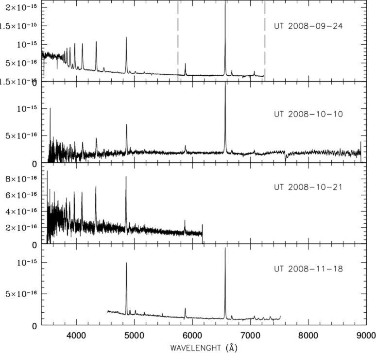
Figure 2: Sample fluxed spectra (ergs/cm²/s/Å) from the spectroscopic observations in Table 1. The UT date of each observing run is indicated in the figure itself. The dashed vertical lines in the top panel delimit the wavelength range of the time series from 27 October. The emission lines in the November 2008 spectrum (bottom panel) redward of 7000Å  are due to second-order overlap (see text).

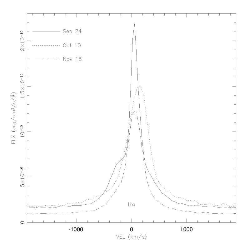
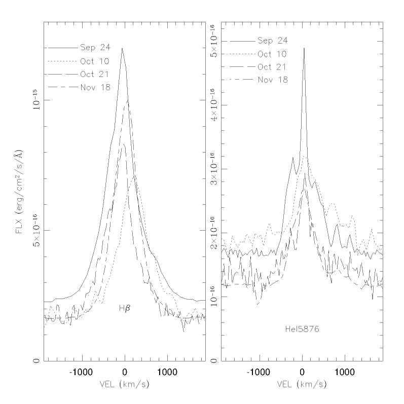
Figure 3: Line profile of H$\alpha$, H$\beta$, and HeI $\lambda$5876 at the various epochs.

4 Analysis of the spectra

4.1 The single spectra

Figure 2 shows that VY Scl low state spectra are dominated by H and HeI emission lines over a slightly blue continuum that culminates in the Balmer jump in emission. By comparison of the line strengths and the 5000Å  continuum level of all the spectra, and of the approximately constant low state V-band magnitude (V$\sim$18.1), we believe that all of our observations sample states of similar mass transfer rate (see Fig. 2). The small flux differences are easily explained by the uncertainties in the calibration intrinsic to slit observations. In particular, a difference in the continuum slope of the 10 October spectrum seems compatible with colour losses due to the fixed east–west orientation of the slit and the timing of the science and the standard star observations.

We compare the line profiles of the Balmer (H$\alpha$ and H$\beta$ and the HeI $\lambda$5876 emission lines in Fig. 3. The majority of the adopted instrument set-ups at the different instruments/telescopes have comparable resolution using grating with 600 lines/mm. The exceptions were the 10 October Goodman spectrum which used a grating with only 300 lines/mm (halving the resolution), and the 27 September FORS2 time series which adopted a grating with 1200 lines/mm. The higher resolution of the latter was capable of separating well the HeI $\lambda$5876 and the Na I D lines. The figure shows that at all times the H and the HeI emission lines are characterised by broad wings extending up to $\sim\pm$1200 km/s from the line centre. Since these broad wings are consistent with accretion disc emission from the analysis of Doppler maps and trailed spectrograms (see Section 4), we must conclude that during this low state at least some of the accretion disc is still present, perhaps with low-level ongoing mass transfer as well. Both the 10 October Goodman spectrum and the 27 September FORS2 time series extend to longer wavelengths, allowing us to detect spectral signatures of the secondary star, for example the redder slope and the TiO absorption band at $\sim$7150Å. In neither case can we properly fit a secondary star template spectrum (due to the low S/N and heavy fringing in one case or to the limited wavelength range in the other). However, the TiO band in the time series allows us to derive the radial velocity of the ‘back’ of the secondary star thus constraining the mass ratio of the binary system (see Sec.4.4).

The higher S/N ratio of the VLT spectra also allow us to identify with certainty the weak emission line from MgI $\lambda$5184 Å. The MgI $\lambda$5167 and 5172 are blended with the FeII $\lambda$5169 Å. The FeII presence is suggested by the fact that the HeI lines at $\sim$4922 and 5015 Å  have somewhat broader full width at half maximum (FWHM) with respect to the HeI at 6678 Å. In addition we detect the CaII K line 3934 Å  in the spectrum from 24 September showing a smaller FWHM (about half that measured on the HeI lines). Following Mason et al. (2008), we ascribe the Mg and Fe emission to the irradiated secondary, and CaII and Na I to stellar activity from a localised region in proximity of the L1 point. Mason et al. ascribed the HeI emission to stellar activity as well. He I emission likely consists of both secondary star and accretion disc/stream contributions since they show substructure and/or multiple components, and their FWHM values are not as narrow as those from MgI and CaII.

4.2 Time series spectroscopy

In both time series spectroscopy runs, all the emission lines appear to be single-peaked while the Balmer and helium lines show broad wings that are not evident in the metal lines. The hydrogen and helium line profiles throughout the orbit are generally complex from centre to wings and best fit by multiple components. We fit them with one narrow Gaussian and one or two additional components with Voigt profiles in order to account for the extended wings. The time-resolved spectral emission lines of the Na i D doublet and Fe ii $\lambda$5169 show profiles that are very different in that they do not contain extended wings or a broad component. Single Gaussians were used to fit these lines.

4.2.1 Orbital period

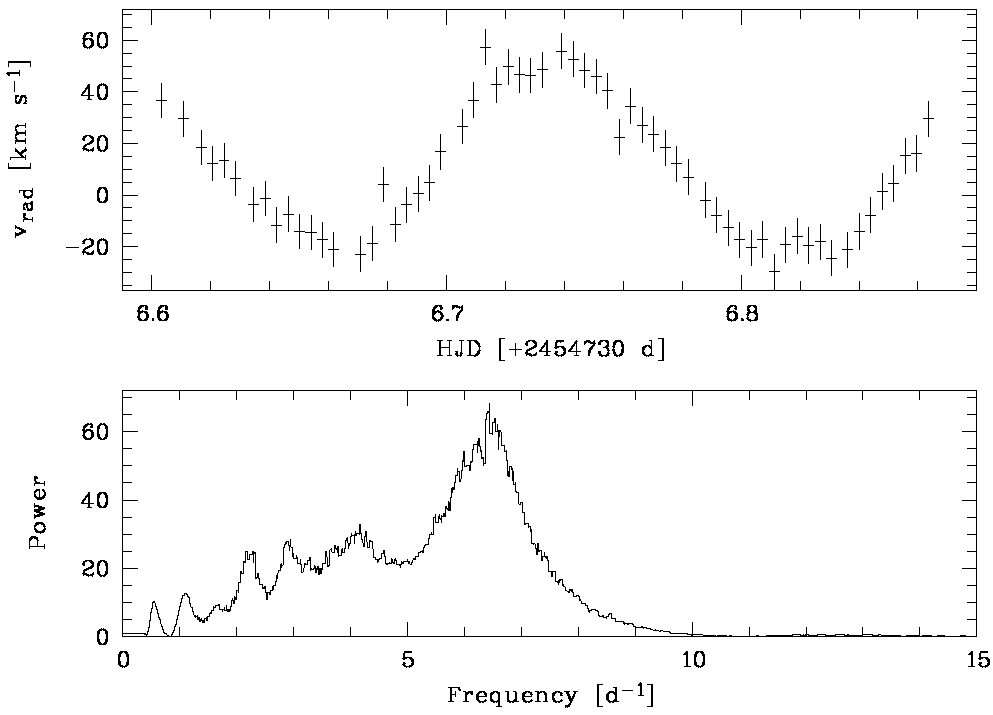
Figure 4: Top: Radial velocity curve of the central H$\alpha$ emission line covering more than one orbit. Bottom: Analysis-of-variance periodogram, the peak centred on 6.35 d^-1. See text for details.

In an attempt to measure the radial velocities and to determine the orbital period, we started with the narrow line components of H and He and fit a Gaussian function to them. These radial velocity measurements show that only the FORS2 run covers more than one orbit and that only the H$\alpha$ emission line, thanks to its higher signal, shows a clear and smooth sinusoidal curve which is suitable for unambiguous period analysis (Fig. 4, top panel). We used the AOV algorithm (Schwarzenberg-Czerny, 1989) as implemented in MIDAS to create a periodogram (see bottom panel of Fig. 4) for H$\alpha$ and, using a Gaussian function, obtained the best fit period of $P_{\rm orb}=3.8\pm 0.3$ h, where the uncertainty corresponds to the $\sigma$ of the Gaussian fit. We note that the periodograms for the other emission lines in the FORS2 data set (i.e. He i 5876, 6678, 7065, and Na i D) are noisier, but they deliver consistent results within their respective uncertainties. We attempted to combine the FORS2 and FORS1 data to increase the accuracy of the orbital period; however, due to the large time difference between the two epochs, we obtained a number of narrow alias peaks all overlapping the area of the broad peak in Fig. 4, which provided no additional constraints.

Past period determinations are those of Hutchings & Cowley (1984) and Martínez-Pais et al. (2000); the former is based on intermediate state spectra (VY Scl was at about V$\sim$16 mag) and the latter on data taken during a high state. The two groups find significantly different orbital periods ($\sim$4.0 and $\sim$5.6 h, respectively), but the best period determined by Hutchings & Cowley (1984) is in relatively good agreement with our determination, given the uncertainties. However, we should note that neither the Hutchings & Cowley (1984) nor the Martínez-Pais et al. (2000) data sets covered a full binary orbit within one night, but combined data from different/consecutive nights. This introduces aliases which can possibly hide the true period. Since our FORS2 data set covers more than a complete orbit continuously, we can plainly rule out the value of $P=5.6$ h by Martínez-Pais et al. (2000).

Looking at the data of Martínez-Pais et al.  in more detail and at the periodogram that they present in the paper, we notice several alias peaks, each of which can correspond to the orbital period. Only one of these peaks, the one at 3.84(3) h, is consistent with our data. Thus, combining our period which is robust but has a large uncertainty with the better defined but less robust period determination of Martinez-Pais et al., we conclude that the orbital period of VY Scl is 3.84(3) h (0.160 d) and adopt this value for all further analyses.

4.2.2 Radial velocity curves

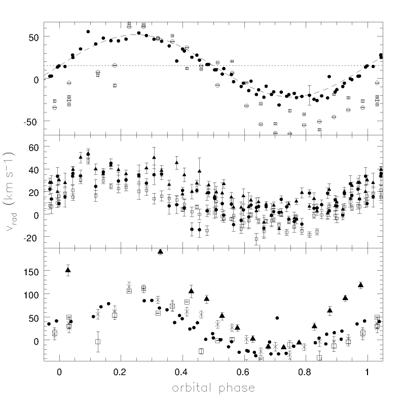
Figure 5: Radial velocity curve of the observed emission lines and the TiO absorption. Top panel: Balmer lines: FORS2 H$\alpha$ measurements are marked by black filled circles, FORS1 H$\alpha$ measurements by empty circles, and FORS1 H$\beta$ measurements by empty squares. Middle panel: Radial velocity of the three HeI emission lines as measured in the FORS2 spectra. Bottom panel: Radial velocity measurements of TiO bandhead (black triangles), NaI D emission (black circles), FeII 5169 blending with MgI (crosses), and MgI 5183 (empty squares).

Table 2: Best fit parameters for the radial velocity curves for each line at each epoch. T_R/B + -2454730 days gives the HJD of the zero phase, defined as the blue-to-red crossing of the central H$\alpha$ line, while $\Delta\phi$ corresponds to the phase offset with respect to this zero phase.

epoch	line ID	K	$\gamma$	TR/B	$\Delta\phi$
		(km/s)	(km/s)
27/09/2008	H$\alpha$	36.8$\pm$0.6	15.0$\pm$0.4	6.6983	0.0
27/09/2008	He i 5875	18.0$\pm$0.7	20.9$\pm$0.5		-0.07
27/09/2008	He i 6678	17.6$\pm$1.0	15.1$\pm$0.7		-0.09
27/09/2008	He i 7065	20.3$\pm$0.9	23.6$\pm$0.6		-0.04
27/09/2008	Na i 5890/6	50.9$\pm$2.3	14.6$\pm$1.5		-0.05
27/09/2008	TiO	114$\pm$20	na $\pm$13		-0.05
18/11/2008	H$\alpha$	56.5$\pm$1.7	-7.0$\pm$1.2	58.6494	0.0
18/11/2008	H$\beta$	45.5$\pm$3.1	-4.7$\pm$2.2		0.03
18/11/2008	Fe ii 5169	57.2$\pm$2.3	-43.6$\pm$1.6		-0.03

The radial velocities of all emission lines were phased using the 3.84 h period determined above and were fit (Fig. 5) with the function $v_{r}(\phi)=\gamma+K\sin{2\pi\phi}$ using a Monte Carlo technique to determine the uncertainties of the individual parameters. The parameters of the best fit for each line are listed in Table 2. We define the epoch of zero-phase as the best fit blue-to-red crossing of the narrow central H$\alpha$ component. This corresponds to $\rm HJD_{0}=2454736.6983(4)\,d$ and $\rm HJD_{0}=2454788.6494(7)\,d$ for the FORS2 and FORS1 run, respectively. The phase offsets in Table 2 have been computed with respect to these ephemerides.

   

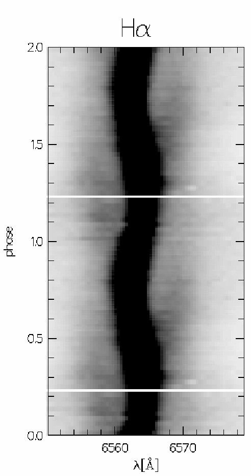
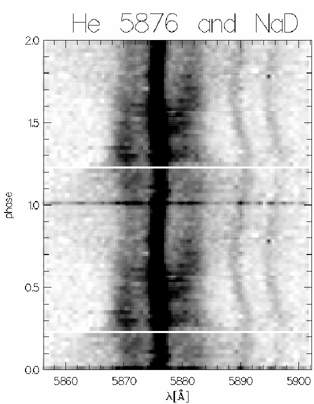
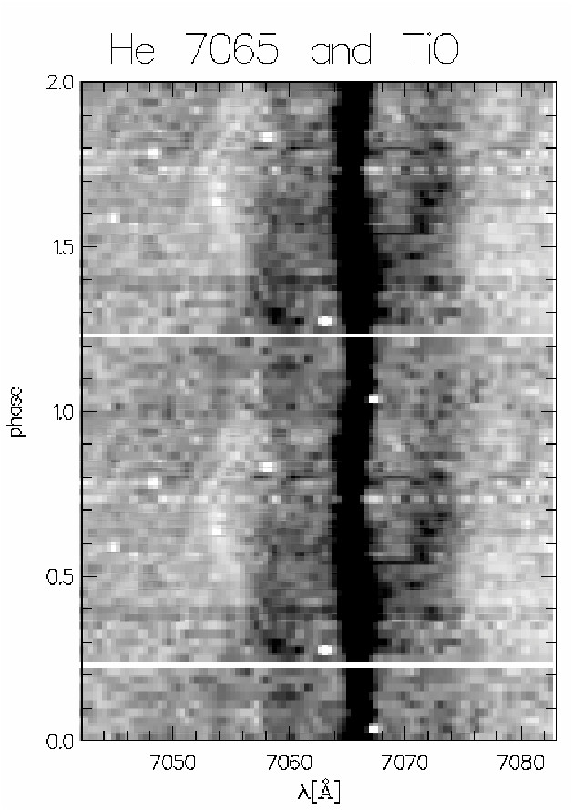
Figure 6: Trailed spectrograms of the FORS2 data showing the regions around H$\alpha$, Hei with Na I D, and Hei with TiO head. The greyscale is inverted, i.e. dark shades of grey represent emission and the TiO absorption appears lighter than the continuum. For clarity, a whole orbital cycle is repeated.

 

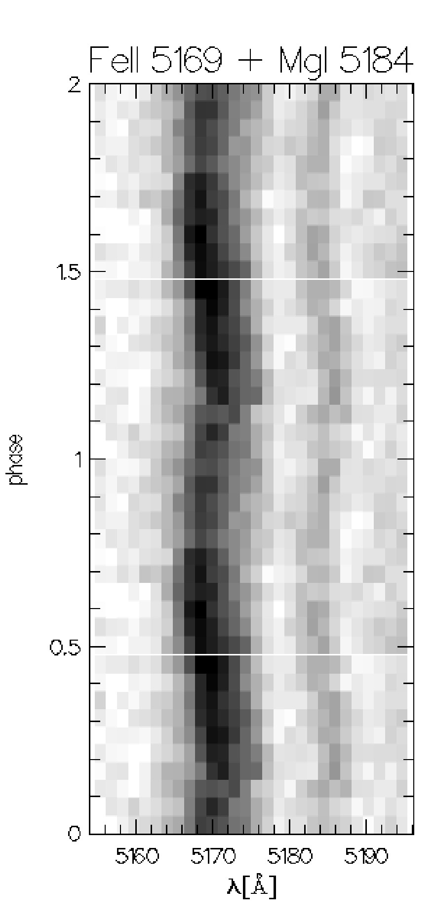
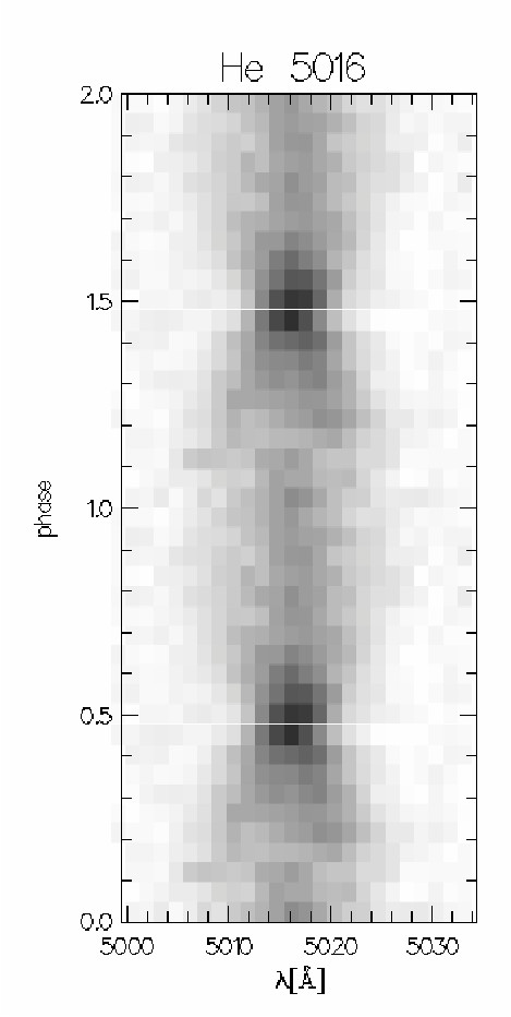
Figure 7: Trailed spectrograms of the FORS1 data showing the different behaviour of the Feii and Hei lines. The weak emission on the red side of the 5169 Å emission is MgI 5184 Å

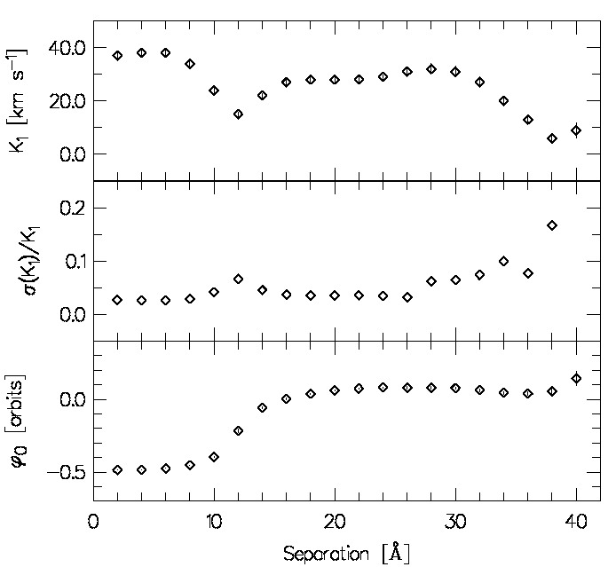
Figure 8: H$\alpha$ diagnostic diagram: radial velocity amplitude $K$, its uncertainty, and the offset of the orbital phase (red to blue crossing yields $\phi_{0}=0$) plotted against the separation of the two Gaussians used for the fitting (see text for details). For small separations, the Gaussians trace the central peak of the emission line and the resulting parameters are close to those listed in Table 2. For separations between 16 and 26 Å, the fitting gives stable parameters while the wings are traced. Further outside, the noise increases and the parameters start varying accordingly.

We note that we did not attempt to fit the radial velocities of the He i lines in the FORS1 data set because at lower resolution the central peaks are severely affected by the broad component/wings. We did, however, fit the weak TiO bandhead at $\sim$7054 Å which we detected on the trailed spectrogram of the He i $\lambda$7065 line (see Fig. 6, right side) and the wings of the H$\alpha$ emission line in the higher resolution FORS2 spectra.

As the TiO absorption cannot be easily spotted in each single spectrum, we measure its radial velocity from the cursor position in the wavelength calibrated trailed image of the spectra. We independently determined the radial velocity in each spectrum seven times and averaged these values together. We note that the TiO absorption was not visible at all orbital phases because of the ‘disturbing’ emission from the He i $\lambda$7065 extended wings. The radial velocity curve of the TiO bandhead is plotted in Fig. 5 and the parameters for the best fit are listed in Table 2. As no precise zero-wavelength could be attributed to the TiO headband, we do not derive a system velocity from the radial velocities of this spectral band and only give the uncertainty in the shift to judge the quality of the fit. In Fig. 6 the trailed spectrogram of the TiO absorption bandhead is plotted in comparison with the various emission lines in the same FORS2 time series.

The radial velocities of the H$\alpha$ line wings were measured using the double-Gaussian fit method described in Schneider & Young (1980) and Shafter (1983). Two Gaussians, each 4 Å in width, were fit to the line profile; the separation of the two Gaussians was varied between 2 and 40 Å. In Fig. 8, the parameters $K$ and $\phi_{0}$ are plotted against the separation of the two Gaussians. We note that the phase offset $\phi_{0}$ in the diagnostic diagram refers to zero phase being the red-to-blue crossing of the line as the diagram is computed to find a radial velocity fit for the primary star. Therefore, $\phi_{0}=-0.5$ indicates that the lines are crossing from blue to red at zero phase $\phi=0$. For small separations, the two Gaussians trace the central peak of the line, and the results of the radial velocity fits are similar to those derived for the radial velocities of the central line that are given in Table 2. For separations between 16 and 26Å, the fitting of the radial velocities gives stable and robust parameters while tracing the outer line wings, values that are a proxy of the white dwarf motion. Averaging over this range, we derive the radial velocity amplitude $K_{1}=29\pm 2\rm\leavevmode\nobreak\ km\,s^{-1}$ and a phase offset of $\phi_{0}=0.06\pm 0.02$.

Similar measurements of the He i line wings in the FORS2 data set did not result in robust fit parameters for any Gaussian separation. This is probably due to a combination of the lower S/N ratio and the stronger variation of the He i emission line wings. As seen from the trailed spectra in Figs. 6 and 7, the He lines are of variable extension and profile across the orbit. For any separation below $\approx 20$ Å the double Gaussian thus traces different emitting regions at different orbital phases. Further outside, where the line is bound to become more stable, the S/N becomes too low for reliable measurements.

4.3 Characterising the distribution of the emission line sources

The analysis of the radial velocity curves and their best fits show that the narrow emission component of H$\alpha$, H$\beta$, He i $\lambda$5876, 6678, and 7065; the Fe ii $\lambda$5169 and Na i D emission lines; and the TiO bandhead absorption all move in phase. As the TiO absorption can clearly be attributed to the secondary star, all of the narrow emission line components also have a likely origin somewhere in the secondary star’s regime. The radial velocity amplitude $K$ is different for all these lines, which implies that they originate from different line emitting regions. The velocity amplitudes follow the series $K_{\rm HeI}<K_{\rm H\alpha}<K_{\rm NaI}<K_{\rm FeII}<K_{\rm TiO}$, a sequence one would expect for a co-rotating, irradiated secondary star with a temperature gradient on its surface. The hottest part of the secondary is the L1 region. This is where He i is emitted, which thus has the smallest radial velocity amplitude. The H$\alpha$ and H$\beta$ line emitting regions will be larger, extending up to colder regions and higher velocities. The coldest region of the secondary star is the non-illuminated backside, where the TiO bands form. Their velocity amplitude is thus expected to have the highest value, which is indeed what we observe.

Temperature gradients in line emitting regions of the secondary are not uncommon among CVs and have been observed, for example in BB Dor during a low state (Schmidtobreick et al., 2012). The BB Dor H$\alpha$, He i, and Na i D narrow emission lines and TiO aborption bands follow a sequence similar to those observed here, and were explained using an irradiation-introduced temperature gradient on the secondary star.

The Na i emission, and possibly the Fe ii or Mg i, are associated with chromospheric activity. They are thus expected to form more or less uniformly all over the active secondary star, and therefore represent the best tracers of the secondary star’s orbital motion (see Howell et al., 2000; Mason et al., 2008)

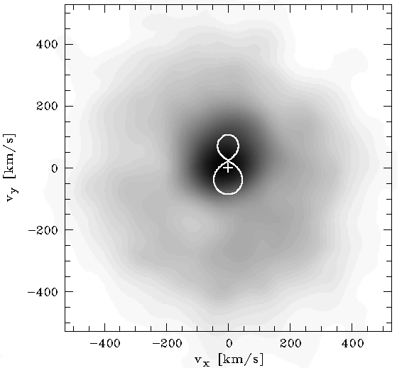
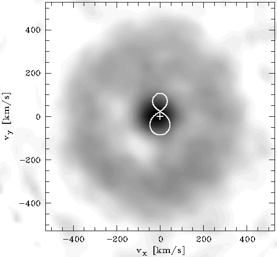
Figure 9: Doppler maps of VY Scl showing the distribution of H$\alpha$ emission (left plot) and the averaged He I emission (right plot) in velocity coordinates. The white cross marks the centre of rotation. The maps are oriented such that the phase angle is zero towards the top and increases clockwise.

From the diagnostic diagram of the H$\alpha$ line (and the discussion above), we determine that the line wings form in a region which is moving exactly anti-phased with respect to the one giving rise to the narrow emission lines. The line wings therefore originate in an approximately symmetric structure on the side of the primary star, likely an accretion disc. In order to better locate this line forming region we apply the Doppler tomography method using the code of Spruit (1998) with a MIDAS interface replacing the original IDL routines (Tappert et al., 2003). Making use of the rotation of the binary system, the calculated Doppler maps $I(v_{x},v_{y})$ display the intensity of the line component emitted at a velocity $(v_{x},v_{y})$. In Fig. 9, the Doppler maps of the H$\alpha$ and He i lines are plotted. Both maps similarly show two features: a strong peak just above the centre of mass and an almost homogeneous ringlike structure. The strong peak is associated with the narrow line components that show the low radial velocity amplitude of the L1 and close-by regions. The ringlike structure in velocity space is the sign of emission from an accretion disc. This is in agreement with the findings of Hamilton & Sion (2008) who also observed VY Scl during a low state (V-magnitude was fainter than 15.8 mag), and found a significant inner accretion disc contribution by modelling the IUE UV spectra.

We point out that the observation of a disc (or at least a small inner disc) is an argument against the ‘no disc option’ proposed by Hameury & Lasota (2002). Hamureuy and Lasota estimate that the value of the magnetic moment necessary to prevent the formation of a disc is in the range between DQ Her and intermediate polars, i.e. $B>6$ MG. Thus, with the observed presence of at least a partial accretion disc, we can rule out a high magnetic field for VY Scl.

4.4 System parameters

A determination of the centre position of each Doppler map yields the velocity amplitude of $K_{1}=28\pm 5\rm\leavevmode\nobreak\ km\,s^{-1}$, a value in good agreement with the value $K_{1}=29\pm 2\rm\leavevmode\nobreak\ km\,s^{-1}$ from the diagnostic diagram. We thus adopt this latter value as the projected velocity $v\sin{i}$ of the white dwarf.

For the secondary star, different values for radial velocity amplitude have been measured depending on the origin of the line emitting region. The velocity amplitude derived from the TiO bands $K_{\rm TiO}=114\pm 20\,\rm km\,s^{-1}$ represents a strict upper limit for the radial velocity amplitude $K_{2}$ of the secondary. For a thorough discussion of the effect of irradiation on the velocity amplitude of absorption lines, see Wade & Horne (1988).

Assuming that the Na i and Fe ii or Mg i emission lines come from chromospheric activity uniformly distributed over the secondary star, they are the best tracers of the secondary star’s orbital motion and we derive $K_{2}=54\pm 3\rm\leavevmode\nobreak\ km\,s^{-1}$ as their average value. However, one might argue that the Na D and Fe II lines can be affected by irradiation and/or that the chromospheric emission sources are clustered towards the L1. In that case, this value would only represent a lower value for the secondary’s radial velocity amplitude.

Approximating the geometry of the elongated, Roche-lobe filling star with an ellipse, we can easily calculate the distance between the secondary’s centre of mass and the binary’s centre of mass as the average of the L1 distance and its backside distance. Since the velocity on a co-rotating structure increases linearly with the distance, we can approximate the velocity at the centre of mass of the secondary as the average between the velocity of L1 and the velocity at the backside of the secondary. The radial velocity of L1 can be estimated as the velocity amplitude $K_{\rm HeI}=19\,\rm km\,s^{-1}$ of the He I line, that of the backside from the $K_{\rm TiO}=114\pm 20\,\rm km\,s^{-1}$. For the secondary’s radial velocity, this approximation yields $K_{2}=67\pm 11\,\rm km\,s^{-1}$. This value is slightly higher than that derived from the chromospheric lines, indicating that the line emitting regions are indeed shifted towards the L1.

Using this geometrically derived radial velocity as the most likely value for the secondary’s orbital motion, we calculate the mass ratio of the binary as $M_{2}/M_{1}=K_{1}/K_{2}=0.43\pm 0.15$. With an estimated secondary star mass of $M_{2}=0.3-0.35$ M_⊙ (Howell et al., 2001, eq.6), we derive the white dwarf mass to $M_{1}=0.5-1.1$ M_⊙ and an inclination around $15^{\circ}$.

5 Summary and conclusions

We observed VY Scl in optical spectroscopy on several epochs during its 2008 low state. At all times, it appears that at least a small inner disc was present. This is supported by the H $\alpha$ and He i Doppler maps that show the disc-like structure around the position of the white dwarf. The presence of such an inner accretion disc in the low state rules out the possibility of VY Scl containing a highly magnetic white dwarf and being an intermediate polar. The TiO absorption bands, the narrow central part of the Balmer and He I emission lines, and the emission lines in Na I and Fe II all move in phase and are anti-phased to the broad H $\alpha$ and He i line wings that result from the accretion disc. Different radial velocity amplitudes of these lines trace the temperature profile on the irradiated secondary.

The time-resolved spectroscopic observations together with old data from Martínez-Pais et al. (2000) allowed us to unambiguously determine the orbital period of the binary: $P=3.84\pm 0.03$ h. We used the broad line wings to trace the white dwarf movement and derived $K_{1}=29\pm 2\,\rm kms^{-1}$. The secondary star shows a temperature gradient as expected from irradiation. From geometric considerations, we derive the most likely value $K_{2}=67\pm 11\,\rm kms^{-1}$ and $M_{2}/M_{1}=0.43$. With the secondary’s mass between 0.3 and 0.35 M_⊙, as expected for a Roche-lobe filling secondary in a $P=3.84$ h-system, we calculate the mass of the white dwarf $M_{1}=0.5-1.1$ M_⊙. With about $15^{\circ}$, the inclination of VY Scl is very low, which makes it difficult to gain any more detailed information from the radial velocities.

References

- Appenzeller et al. (1998) Appenzeller, I., Fricke, K., Fürtig, W., et al. 1998, Messenger, 94, 1
- Burrell & Mould (1973) Burrell, J. F. & Mould, J. R. 1973, PASP, 85, 627
- Clemens et al. (2004) Clemens, J. C., Crain, J. A., & Anderson, R. 2004, in Society of Photo-Optical Instrumentation Engineers (SPIE) Conference Series, Vol. 5492, Society of Photo-Optical Instrumentation Engineers (SPIE) Conference Series, ed. A. F. M. Moorwood & M. Iye, 331–340
- Dworetsky (1983) Dworetsky, M. M. 1983, MNRAS, 203, 917
- Hameury & Lasota (2002) Hameury, J. M. & Lasota, J. P. 2002, A&A, 394, 231
- Hameury & Lasota (2005) Hameury, J.-M. & Lasota, J.-P. 2005, A&A, 443, 283
- Hamilton & Sion (2008) Hamilton, R. T. & Sion, E. M. 2008, PASP, 120, 165
- Horne (1986) Horne, K. 1986, PASP, 98, 609
- Howell (2004) Howell, S. B. 2004, in Astronomical Society of the Pacific Conference Series, Vol. 315, IAU Colloq. 190: Magnetic Cataclysmic Variables, ed. S. Vrielmann & M. Cropper, 353
- Howell et al. (2000) Howell, S. B., Ciardi, D. R., Dhillon, V. S., & Skidmore, W. 2000, ApJ, 530, 904
- Howell et al. (2001) Howell, S. B., Nelson, L. A., & Rappaport, S. 2001, ApJ, 550, 897
- Hutchings & Cowley (1984) Hutchings, J. B. & Cowley, A. P. 1984, PASP, 96, 559
- King & Cannizzo (1998) King, A. R. & Cannizzo, J. K. 1998, ApJ, 499, 348
- Leach et al. (1999) Leach, R., Hessman, F. V., King, A. R., Stehle, R., & Mattei, J. 1999, MNRAS, 305, 225
- Livio & Pringle (1994) Livio, M. & Pringle, J. E. 1994, ApJ, 427, 956
- Luyten & Haro (1959) Luyten, W. J. & Haro, G. 1959, PASP, 71, 469
- Martínez-Pais et al. (2000) Martínez-Pais, I. G., Martín-Hernández, N. L., Casares, J., & Rodríguez-Gil, P. 2000, ApJ, 538, 315
- Mason et al. (2008) Mason, E., Howell, S. B., Barman, T., Szkody, P., & Wickramasinghe, D. 2008, A&A, 490, 279
- Rodríguez-Gil et al. (2012) Rodríguez-Gil, P., Schmidtobreick, L., Long, K. S., et al. 2012, MNRAS, 422, 2332
- Rodríguez-Gil et al. (2015) Rodríguez-Gil, P., Shahbaz, T., Marsh, T. R., et al. 2015, MNRAS, 452, 146
- Scargle (1981) Scargle, J. D. 1981, ApJS, 45, 1
- Schmidtobreick (2015) Schmidtobreick, L. 2015, in The Golden Age of Cataclysmic Variables and Related Objects - III (Golden2015), 34
- Schmidtobreick et al. (2012) Schmidtobreick, L., Rodríguez-Gil, P., Long, K. S., et al. 2012, MNRAS, 422, 731
- Schneider & Young (1980) Schneider, D. P. & Young, P. 1980, ApJ, 238, 946
- Schwarzenberg-Czerny (1989) Schwarzenberg-Czerny, A. 1989, MNRAS, 241, 153
- Shafter (1983) Shafter, A. W. 1983, ApJ, 267, 222
- Spruit (1998) Spruit, H. C. 1998, ArXiv Astrophysics e-prints: astro-ph/9806141
- Tappert et al. (2003) Tappert, C., Mennickent, R. E., Arenas, J., Matsumoto, K., & Hanuschik, R. W. 2003, A&A, 408, 651
- Wade & Horne (1988) Wade, R. A. & Horne, K. 1988, ApJ, 324, 411
- Walter et al. (2012) Walter, F. M., Battisti, A., Towers, S. E., Bond, H. E., & Stringfellow, G. S. 2012, PASP, in press
- Warner (1995) Warner, B. 1995, Cataclysmic Variable Stars (Cambridge: Cambridge University Press)
- Warner (1999) Warner, B. 1999, in Annapolis Workshop on Magnetic Cataclysmic Variables,, ed. C. Hellier & K. Mukai (ASP Conf. Ser. 157), 63–70
- Warner & van Citters (1974) Warner, B. & van Citters, G. W. 1974, The Observatory, 94, 116